Acoustic Noise of Induction Motor Drive with Voltage-Source Inverter by Random Space Vector PWM: Simulation and Experimentation Analysis

Abstract

The discrete tonal bands generated by an electric machine stator current spectrum for the fixed Space Vector Pulse Width Modulation (SVPWM) control have side effects on the acoustic noise and vibration. Thus, reducing the magnitude of dominant harmonics and spreading the harmonic spectrum provide a remedy for this problem. A well-established concept has involved the application of the randomized Pulse Width Modulation (PWM) strategy in power converters to spread the power spectrum of the stator current to minimize its amplitude. Therefore, Random SVPWM (RSVPWM) is a new switching method applied for power converters. For the control of the three-phase inverter, three different RSVPWM approaches are suggested: Random Switching Frequency (RSF), Random Zero Vector (RZV) and Random Pulse Position (RPP). This paper investigates the effect of the fixed and random SVPWM strategies on acoustic noise emitted by an Induction Machine (IM) fed by a three-phase inverter. Simulation results exhibit the validity and efficiency of the RSF_SVPWM strategy to reduce sideband harmonics at different modulation indexes. The proposed PWM strategies evaluate the results of the equivalent experiments on an IM fed by a two-level voltage source inverter. The experimental results of the harmonic current and acoustic noise spectra demonstrate also that the acoustic noise is attenuated and dispersed totally for the proposed RSF_SVPWM compared to the RZV_SVPWM and, RPP_SVPWM strategies and the random PWM modulation.

1. Introduction

Induction Machines (IMs) are promising electrical motors used in industry and for electric vehicles thanks to their performance, high efficiency, low cost and almost free maintenance. Recently, the systems including power converters and electric motors have been widely used for electric vehicles. The acoustic noise generated by the IM drive as a variable-speed drive becomes a problem for the living environment, and even a slight noise may cause discomfort. The audible range of humans is generally from 20 Hz to 20 kHz. In recent years, the acoustic noise emitted by electric motors has been the subject of numerous studies. The acoustic noise sources can be grouped into four types: mechanic, aerodynamic, magnetic, and electronic [1,2,3]. Our work focuses on the study of electronic noise and accordingly in switching harmonics sources. The flux harmonics in the air gap of an IM create radial forces in the stator frame. Thus, these harmonics cause excitation forces that have a detrimental effect on the machine structure. Consequently, the considerable emission of vibration and noise can be engendered, which makes the machine more troublesome to operate. Generally, there are three main reasons for the harmonics in the air-gap flux reported in the literature:

• Spatial harmonics due to the non-sinusoidal repartition of coils in the stator and the rotor.
• Harmonics in the air-gap permeance, which depend on the number and geometry of the stator and rotor slots, the geometry of the teeth in both the stator and the rotor, and the permeation in the iron core.
• Harmonic current in the stator coil.

IM-driven solid-state inverter drive systems are full of harmonics since their power voltages are non-sinusoidal. The harmonics absorbed by the stator coils generate additional stator flux density components—hence the additional force waves to be produced. Voltage-Source Inverter (VSI)-fed IMs produce disagreeable acoustic noise caused by current harmonics at the inverter output. Consequently, these harmonics are narrow-band components located around the inverter switching frequency and its multiples. Furthermore, an analysis of the harmonic spectrum of the voltage or current can determine and define the frequencies and amplitudes of the different harmonics at the inverter output. In fact, noise intensity depends on the harmonic spectrum of the inverter output, which is also correlated to the Pulse Width Modulation (PWM) strategy control applied to the inverter. Motor drives modulated with such PWM methods invariably emit discrete/tonal noise, which is irritating to the human ear. Numerous PWM techniques have been developed and proposed in the literature. Sine PWM (SPWM) and Space Vector PWM (SVPWM) are well-known fixed-switching frequency PWM methods applied in industry. Using the SPWM strategy, the inverter harmonic is concentrated in distinct zones located around the switching frequency and its integer multiples. However, the SVPWM strategy has the advantage of high voltage utilization and can offer reduced current. Moreover, the harmonics are decreased and are concentrated around the integer multiples of the VSI switching frequency compared to the SPWM strategy. The acoustic noise emitted by an IM fed by a PWM inverter remains very interesting, considering the numerous articles published lately. The author in [4,5] elaborated on an experimental procedure to determine the acoustic and vibration behavior of SVPWM-modulated IM drives over a range of carriers and modulation frequencies. An advanced SVPWM scheme with a special type of switching sequence was also reported in [6] to reduce the acoustic noise in low and medium-speed ranges of the motor drive. A lot of researchers have recently published and investigated the Random PWM (RPWM) technique in order to reduce the tonal bands around the multiple of the switching frequency with fixed PWM and disperse them over a wide range of frequencies.

Numerous randomization schemes like the Random Switching Frequency (RSF), the Random Zero Vector (RZV) and the Random Pulse Position (RPP) have been lately published for DC-DC (chopper) and DC-AC (inverter) converters [7,8,9,10,11,12,13,14]. The author in [7] proposed a novel Hybrid RPWM (HRPWM) technique based on modified SVPWM for three-phase VSIs to eliminate the PWM acoustic noise. The proposed HRPWM technique could remove the unpleasant acoustic high-frequency noise more effectively than fixed PWM with lower switching losses and a shorter random frequency range. The effects of the SVPWM, Selective Harmonic Elimination PWM (SHEPWM) and RPWM strategies were developed in [8]. The acoustic noise emitted by a two-level inverter-fed IM and a harmonic spectrum were carried out corresponding to the three PWM techniques at different conditions. Consequently, the experimental results showed that the acoustic noise and the harmonic spectrum were significantly reduced with the RPWM strategy. Nowadays, a lot of researchers have published and investigated the random SVPWM strategy effect in terms of acoustic noise emitted by an electric motor [15,16,17,18,19,20,21]. SVPWM is very well considered in industry as regards the higher DC bus utilization and the superior waveform properties compared to other PWM techniques. Based on the switching signal for VSI modulated with the SVPWM technique, three parameters can be randomized. The three randomization schemes are the RSF, the RZV, and the RPP. For the three-phase inverter, the switching signals are generated by comparing three deterministic reference signals to a triangular carrier with random parameters.

This paper presents the simulation and experimental implementation of the fixed SVPWM and three random SVPWM schemes: RSF_SVPWM, RZV_SVPWM and RPP_SVPWM. The investigation of spectral characteristics in terms of harmonic spectra and acoustic noise emitted by an IM is studied and discussed. Therefore, this document is structured as follows: Section 2 presents the description of acoustic noise in electric machines. In Section 3, the principles of advanced SVPWM techniques are presented. In Section 4, the two-level PWM inverter and the IM are applied using Simulink, and the obtained simulation results are presented and discussed. An experimental setup of an PWM inverter and an IM is presented in Section 5, and the experimental tests of emitted noise are given and discussed. Some general conclusions are provided in Section 6.

2. Acoustic Noise Sources of Electric Machines

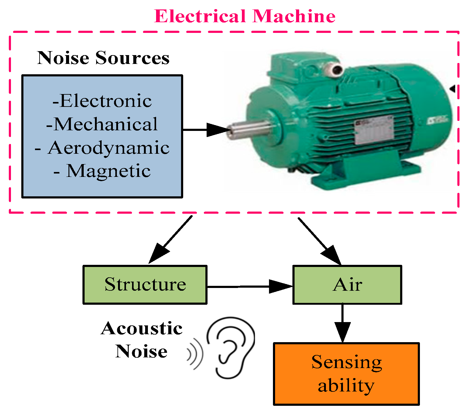
For several years, the search to guarantee the best operating performance for an IM powered by static converters has been the subject of numerous research and development projects. Electrical machines, including IMs, constitute major noise sources in industry. Noise exposure leads to psycho-acoustic and health problems for human beings. Figure 1 demonstrates the mechanism for generating noise in an electrical machine. Thus, this system is characterized, on the one hand, by the noise source (electric motor) as a principal cause of acoustic phenomena and, on the other hand, by the elements related to perception and sensation by the human ear. The overall noise level in an electrical machine originates from four main sources. Considerable efforts have been made to identify the acoustic noise sources of an electrical machines [1,2,3,22]. These can be further subdivided into four main sources: electronic, mechanical, magnetic and aerodynamic. These sources provide also the excitation forces that act on the internal structure of the stator core. The pressure of the ambient air varies periodically under the effect of vibrations, and this creates noise. Consequently, the sound wave is audible to the human ear. In this study, electronic noise, as well as its switching harmonics, are studied.

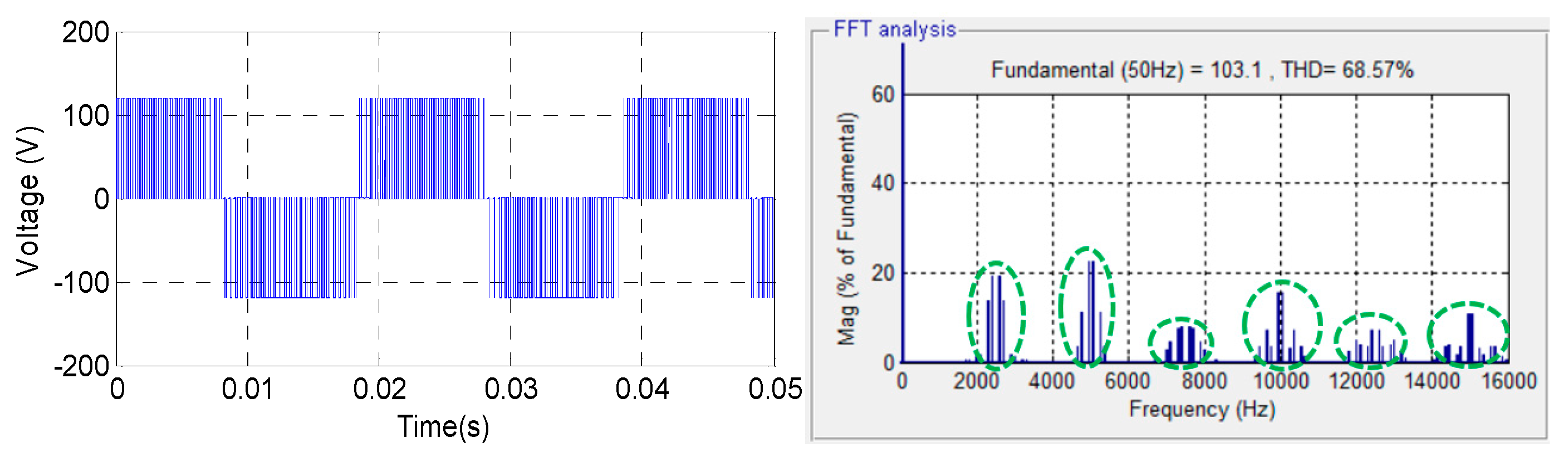
A voltage inverter produces voltages containing harmonics, which can cause considerable noise, particularly when their frequencies are close to those proper to the machine. Furthermore, the harmonics absorbed by the stator windings produce additional stator flux density components, hence generating other magnetic force components. The frequency of voltage harmonics can be obtained as follows:

$${\mathrm{F}}_{\mathrm{n}}=\left|{\mathrm{n}}_1{\mathrm{F}}_{\mathrm{c}}+{\mathrm{n}}_2\mathrm{F}\right|$$

(1)

where F is the fundamental frequency, ${\mathrm{F}}_{\mathrm{c}}$ is the switching frequency, and n₁ and n₂ are integers.

An example of voltage waveform at the output of a three-phase inverter and its Fast Fourier Transform (FFT) for an ${\mathrm{F}}_{\mathrm{c}}$ switching frequency of 2.5 kHz are presented in Figure 2. The harmonic components are distributed in groups of sidebands near the switching frequency, and its multiple is shown.

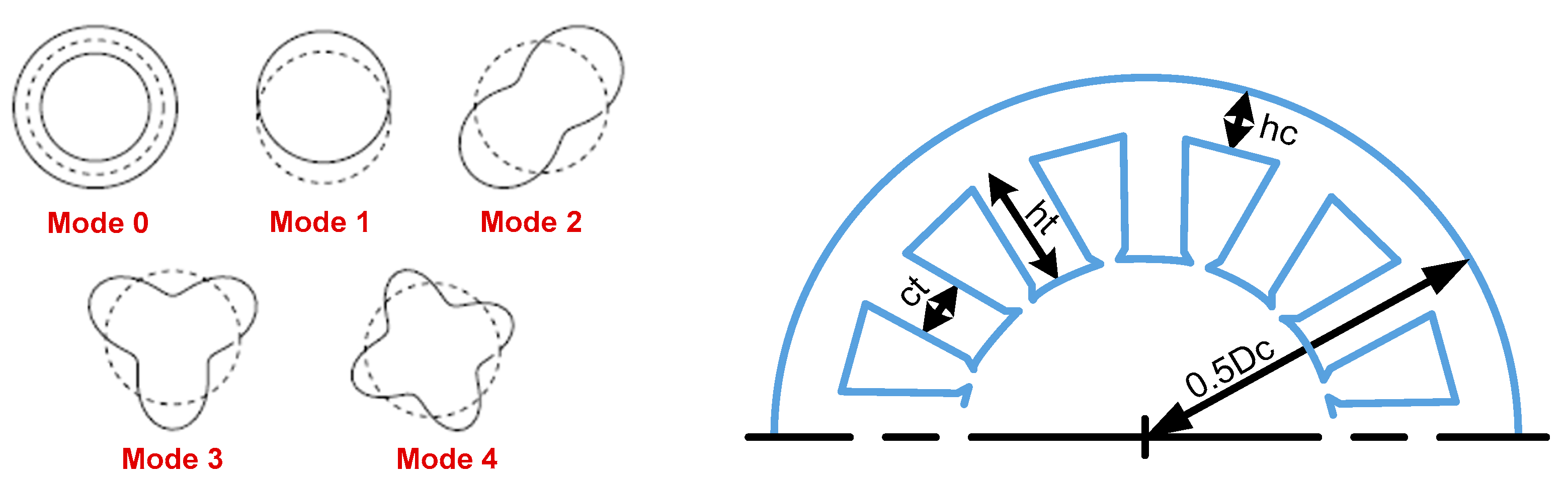
In electric machines, the harmonics components in the air gap generate radial forces applied to the stator, tending to dynamically deform its structure. In this way, the stator is stressed by multiple deflections. Generally, the mechanical behavior of the machine stator can be characterized by its natural modes of vibration. Each mode, corresponding to a proper frequency, represents a particular deformation of the structure [8]. When designing electric rotating machinery, it is essential to take into account both the frequencies of the applied forces and the proper frequencies of the stator system. Various vibration modes (0, 1, 2, 3...) are linked to the natural frequencies, and they are the lower modes that significantly influence the increase in electromagnetic noise. Figure 3 illustrates the spatial distribution of forces generating vibration modes of different orders (m = 0, 1, 2, 3, 4) and the geometry of the stator ring and the teeth.

Equation (2) gives the natural frequency ${\mathrm{F}}_0$ of the order vibration mode m = 0 [8]:

$${\mathrm{F}}_0={\displaystyle \frac{1}{\mathsf{\pi }{\mathrm{D}}_{\mathrm{c}}}}\sqrt{{\displaystyle \frac{{\mathrm{E}}_{\mathrm{c}}}{{\mathsf{\rho }}_{\mathrm{c}}{\mathrm{k}}_{\mathrm{i}}{\mathrm{k}}_{\mathrm{m}\mathrm{d}}}}}$$

(2)

where ${\mathrm{D}}_{\mathrm{c}}$ is the average diameter of the stator core, ${\mathrm{E}}_{\mathrm{c}}$ is the elasticity modulus, ${\mathsf{\rho }}_{\mathrm{c}}$ is the density, ${\mathrm{k}}_{\mathrm{i}}$ is the piling factor, and ${\mathrm{k}}_{\mathrm{m}\mathrm{d}}$ is the mass addition factor for the displacement.

The natural frequency F₁ of the first-order vibration mode m = 1 is expressed by

$${\mathrm{F}}_1={\mathrm{F}}_0\sqrt{{\displaystyle \frac{2}{1+{\mathrm{k}}^2\frac{{\mathrm{k}}_{\mathrm{m}\mathrm{r}\mathrm{o}\mathrm{t}}}{{\mathrm{k}}_{\mathrm{m}\mathrm{d}}}}}}$$

(3)

where ${\mathrm{k}}_{\mathrm{m}\mathrm{r}\mathrm{o}\mathrm{t}}$ is the mass addition factor, $\mathrm{k}={\displaystyle \frac{{\mathrm{h}}_{\mathrm{c}}}{\sqrt{3}{D}_c}}$, and ${\mathrm{h}}_{\mathrm{c}}$ is the stator thickness.

$${\mathrm{k}}_{\mathrm{mrot}}=1+{\displaystyle \frac{{\mathrm{s}}_{\mathrm{l}}{\mathrm{c}}_{\mathrm{t}}{\mathrm{L}}_{\mathrm{i}}{\mathrm{h}}_{\mathrm{t}}^2}{\mathsf{\pi }{\mathrm{D}}_{\mathrm{c}}{\mathrm{I}}_{\mathrm{c}}}}\left(1+{\displaystyle \frac{{\mathrm{M}}_{\mathrm{w}}+{\mathrm{M}}_{\mathrm{i}}}{{\mathrm{M}}_{\mathrm{t}}}}\right)\left(4{\mathrm{h}}_{\mathrm{t}}^2+6{\mathrm{h}}_{\mathrm{c}}{\mathrm{h}}_{\mathrm{t}}+3{\mathrm{h}}_{\mathrm{c}}^2\right)$$

(4)

where ${\mathrm{s}}_{\mathrm{l}}$ is the stator tooth number, ${\mathrm{c}}_{\mathrm{t}}$ is the tooth width, ${\mathrm{h}}_{\mathrm{t}}$ is the tooth height, ${\mathrm{M}}_{\mathrm{t}}$ is the mass of the stator teeth, ${\mathrm{M}}_{\mathrm{w}}$ is the mass of the stator windings, ${\mathrm{M}}_{\mathrm{i}}$ is the insulation mass, and ${\mathrm{I}}_{\mathrm{c}}$ is the surface moment of inertia near the axis parallel to the cylinder axis.

Generally, the expression of the natural frequencies ${\mathrm{F}}_{\mathrm{m}}$ of the vibration mode m ≥ 2 is defined by

$${\mathrm{F}}_{\mathrm{m}}={\mathrm{F}}_0\mathrm{k}{\displaystyle \frac{\mathrm{m}\left({\mathrm{m}}^2-1\right)}{\sqrt{{\mathrm{m}}^2+1}}}{\mathrm{f}}_{\mathrm{m}}$$

(5)

The expression of f_m is defined as follows:

$${\mathrm{f}}_{\mathrm{m}}={\left(1+{\displaystyle \frac{{\mathrm{k}}^2\left({\mathrm{m}}^2-1\right)\left[{\mathrm{m}}^2\left(4+\frac{{\mathrm{k}}_{\mathrm{m}\mathrm{r}\mathrm{o}\mathrm{t}}}{{\mathrm{k}}_{\mathrm{m}\mathrm{d}}}\right)+3\right]}{{\mathrm{m}}^2+1}}\right)}^{-1/2}$$

(6)

3. Random SVPWM

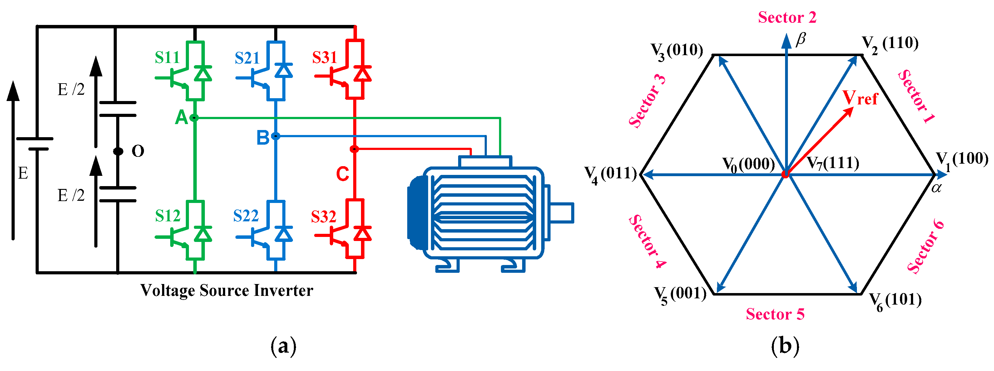
The power circuit structure of a two-level VSI supplying an IM is also depicted in Figure 4a. SVPWM is a digital technique based on the representation of three reference voltages by a single space vector. For the two-level inverter, eight possible combinations of power switch states yield eight vectors whose two vectors are inactive because they are identically zero. The six non-zero vectors in the plane (α, β) are given in the form of a standard hexagon whose origin is aligned to the zero vectors, as shown in Figure 4b.

The general expressions for reference voltages of amplitude V_m are given by the system of Equations (7):

$$\left\{\begin{array}{l}{\mathrm{V}}_{\mathrm{A}\mathrm{r}\mathrm{e}\mathrm{f}}={\mathrm{V}}_{\mathrm{m}}\sin \left(2\mathsf{\pi }\mathrm{F}\mathrm{t}\right)\\ {\mathrm{V}}_{\mathrm{B}\mathrm{r}\mathrm{e}\mathrm{f}}={\mathrm{V}}_{\mathrm{m}}\sin \left(2\mathsf{\pi }\mathrm{F}\mathrm{t}-{\displaystyle \frac{2\mathsf{\pi }}{3}}\right)\\ {\mathrm{V}}_{\mathrm{C}\mathrm{r}\mathrm{e}\mathrm{f}}={\mathrm{V}}_{\mathrm{m}}\sin \left(2\mathsf{\pi }\mathrm{F}\mathrm{t}-{\displaystyle \frac{4\mathsf{\pi }}{3}}\right)\end{array}\right.$$

(7)

where ${\mathrm{V}}_{\mathrm{m}}={\displaystyle \frac{{\mathrm{i}}_{\mathrm{m}}{\mathrm{V}}_{\mathrm{d}\mathrm{c}}}{2}}$ is the amplitude of the sine wave, and ${\mathrm{i}}_{\mathrm{m}}$ is the modulation index.

Vector V₀ is applied during a duty cycle noted d₀, and the two adjacent active vectors V₁ and V₂ are applied, respectively, during the cyclic ratios d₁ and d₂. The general expressions for the duty cycles d₀, d₁ and d₂ are given by:

$$\left\{\begin{array}{l}{\mathrm{d}}_1={\displaystyle \frac{\sqrt{3}{\mathrm{V}}_{\mathrm{r}\mathrm{e}\mathrm{f}}}{\mathrm{E}}}\sin \left(\mathrm{s}{\displaystyle \frac{\mathsf{\pi }}{3}}-\mathsf{\theta }\right)\\ {\mathrm{d}}_2={\displaystyle \frac{\sqrt{3}{\mathrm{V}}_{\mathrm{r}\mathrm{e}\mathrm{f}}}{\mathrm{E}}}\sin \left(\mathsf{\theta }-\left(\mathrm{s}-1\right){\displaystyle \frac{\mathsf{\pi }}{3}}\right)\\ {\mathrm{d}}_0=1-\left({\mathrm{d}}_1+{\mathrm{d}}_2\right)\end{array}\right.$$

(8)

where $\mathsf{\theta }$ represents the instantaneous angle, s is the sector, and V_ref is the reference space vector.

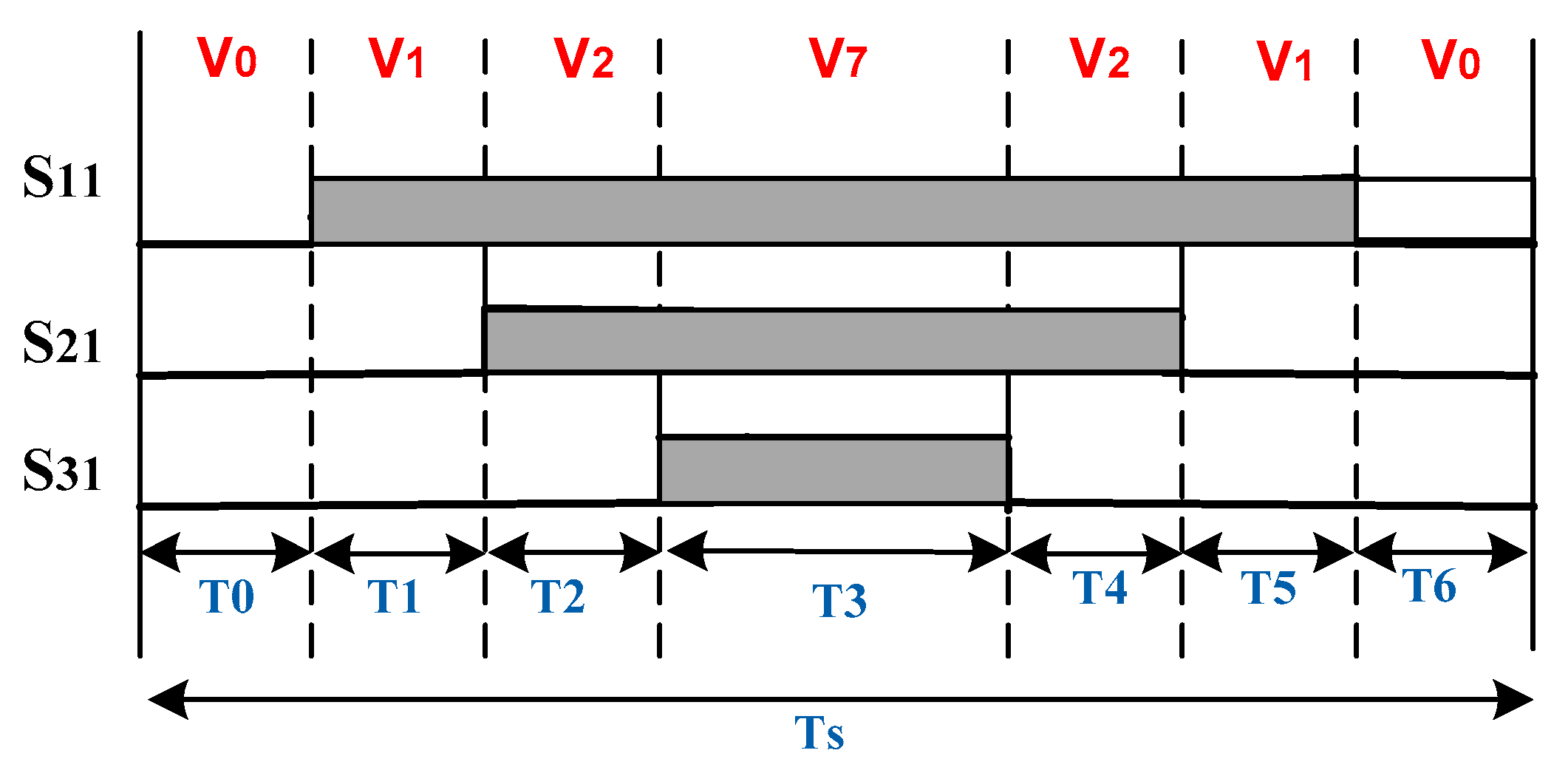
The SVPWM algorithm subdivides sectors and transforms the reference vector into active vectors, which is demonstrated in Figure 4. The SVPWM strategy is performed by rotating the space vector. Thus, the control signals are elaborated by determining the sector number and calculating the duty cycles. The triangular carrier wave for the fixed SVPWM algorithm widely adopts the up–down counting mode of the timer. During the PWM modulation process, the modulation wave and the carrier wave are compared at a fixed switching frequency. The three-phase inverter requires three switching signals: S11, S21 and S31. The switching state distribution where the reference voltage V_ref is positioned in the first sector is explained in Figure 5.

The durations of switching signals for the SVPWM control are obtained and computed using the following relations:

$$\left\{\begin{array}{l}{\mathrm{T}}_0={\mathrm{T}}_6={\displaystyle \frac{{\mathrm{d}}_0}{2}}\\ {\mathrm{T}}_1={\mathrm{T}}_5={\displaystyle \frac{{\mathrm{d}}_1}{2}}\\ {\mathrm{T}}_2={\mathrm{T}}_4={\displaystyle \frac{{\mathrm{d}}_2}{2}}\\ {\mathrm{T}}_3=2\times {\mathrm{T}}_6=2\times {\mathrm{T}}_0={\displaystyle \frac{{\mathrm{d}}_0}{2}}\end{array}\right.$$

(9)

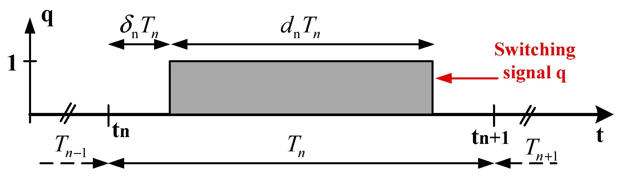
Figure 6 displays the general case of a switching signal q for a three-phase VSI, which can be characterized by three parameters: the switching period T, the duty cycle d and the delay report δ.

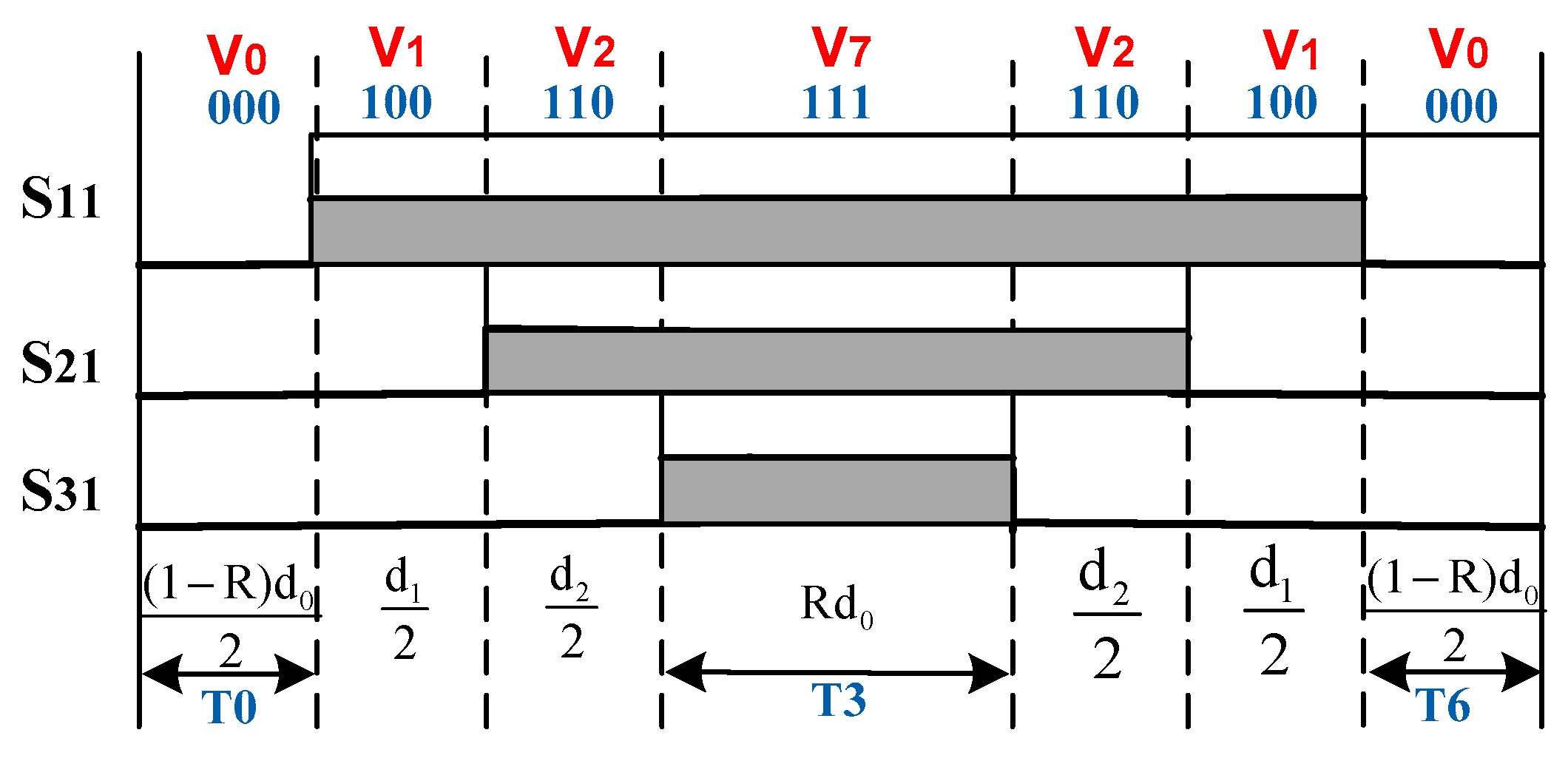
Furthermore, three advanced random SVPWM algorithms can be obtained, such as RZV_SVPWM, RPP_SVPWM, and RSF_SVPWM. The RZV_SVPWM control consists of making period T and delay report δ deterministic and duty cycle d random [10,11,12]. Figure 7 displays the switching state distribution at sector 1 for RZV_SVPWM control. The zero voltage vectors randomize the zero voltage vectors V₇ and V₀. The sum of durations (T₀ + T₆) of the zero vector state V₀ is complementary to that of the zero voltage vector V₇ during period T₃. Thus, durations T₃, T₀ and T₆ are determined as follows:

$$\left\{\begin{array}{l}{\mathrm{T}}_3=\mathrm{R}{\mathrm{d}}_0\\ {\mathrm{T}}_0={\mathrm{T}}_6=(1-\mathrm{R}){\displaystyle \frac{{\mathrm{d}}_0}{2}}\end{array}\right.$$

(10)

where R is a random number between 0 and 1.

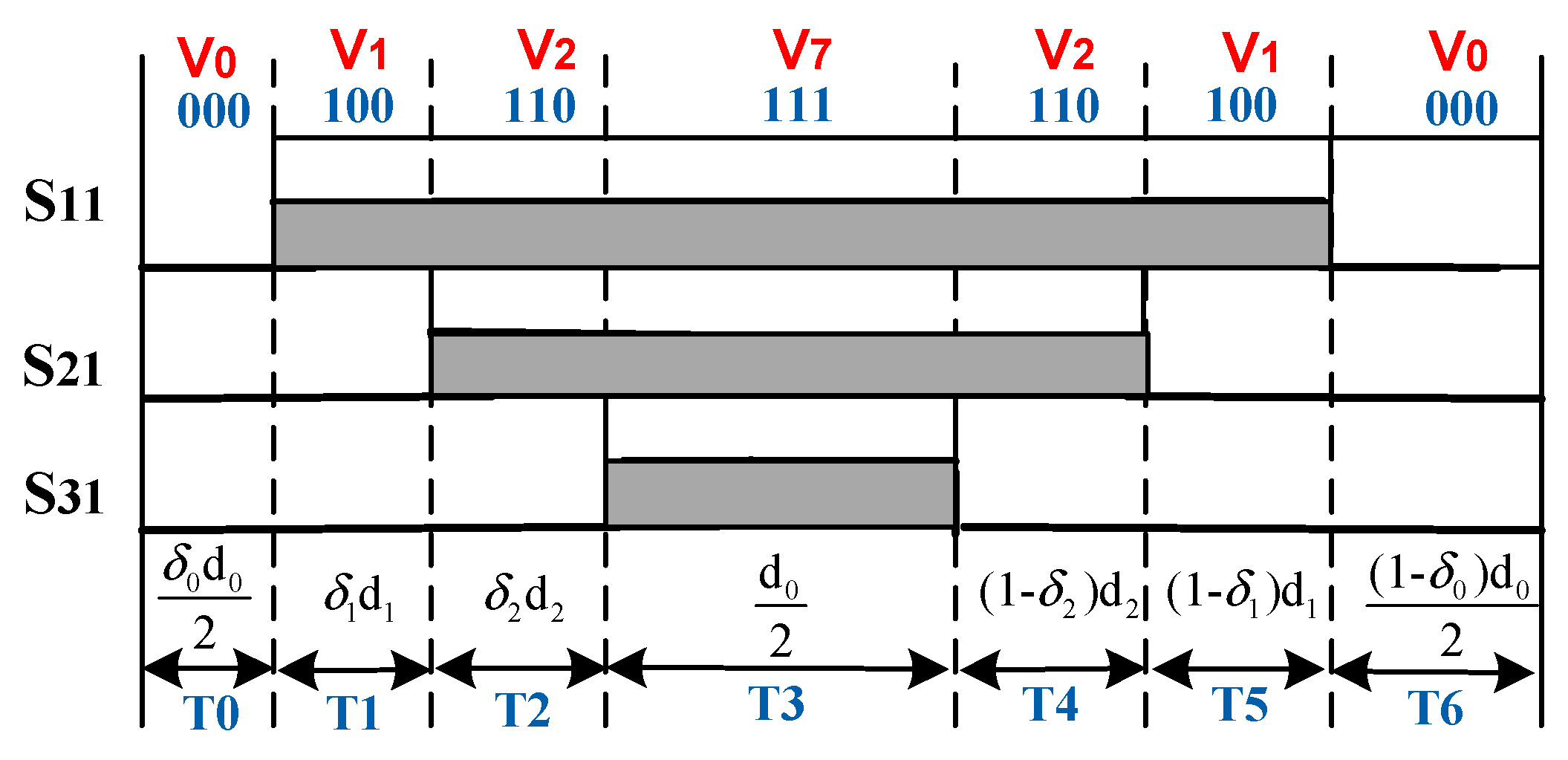
Figure 8 shows the switching pulses at sector 1 for the RPP_SVPWM control. Period T and duty cycle d of the switching signal are deterministic, and delay report δ is random. Consequently, the pulse positions are randomized by varying the durations of vectors states V₀, V₁ and V₂, respectively, using the random parameters δ₀, δ₁ and δ₂ [10,11,12].

According to random parameters δ₀, δ₁ and δ₂, the durations expressions are defined by

$$\left\{\begin{array}{l}{\mathrm{T}}_0={\mathsf{\delta }}_0{\displaystyle \frac{{\mathrm{d}}_0}{2}}\\ {\mathrm{T}}_1={\mathsf{\delta }}_1{\mathrm{d}}_1\\ {\mathrm{T}}_2={\mathsf{\delta }}_2{\mathrm{d}}_2\\ {\mathrm{T}}_3={\displaystyle \frac{{\mathrm{d}}_0}{2}}\\ {\mathrm{T}}_4=(1-{\mathsf{\delta }}_2){\mathrm{d}}_2\\ {\mathrm{T}}_5=(1-{\mathsf{\delta }}_1){\mathrm{d}}_1\\ {\mathrm{T}}_6=(1-{\mathsf{\delta }}_0){\displaystyle \frac{{\mathrm{d}}_0}{2}}\end{array}\right.$$

(11)

The variation interval for random parameter δ_i (i = 0, 1, 2) is given by:

$${\mathsf{\delta }}_{\mathrm{i}}\in \left[\overline{\mathsf{\delta }}\left(1-{\displaystyle \frac{{\mathrm{R}}_{\mathsf{\delta }}}{2}}\right),\overline{\mathsf{\delta }}\left(1+{\displaystyle \frac{{\mathrm{R}}_{\mathsf{\delta }}}{2}}\right)\right],\hspace{1em}\mathrm{i}=0,1,2.$$

(12)

where $\overline{\mathsf{\delta }}={\displaystyle \frac{1}{2}}$ is the statistical mean of random parameter δ_i, and ${\mathrm{R}}_{\mathsf{\delta }}={\displaystyle \frac{{\mathsf{\delta }}_{\max }-{\mathsf{\delta }}_{\min }}{\overline{\mathsf{\delta }}}}$ is the randomness level. Theoretically, ${\left({\mathrm{R}}_{\mathsf{\delta }}\right)}_{\max }=2$. Indeed, ${\mathsf{\delta }}_{\mathrm{i}}$ is also a random number between 0 and 1.

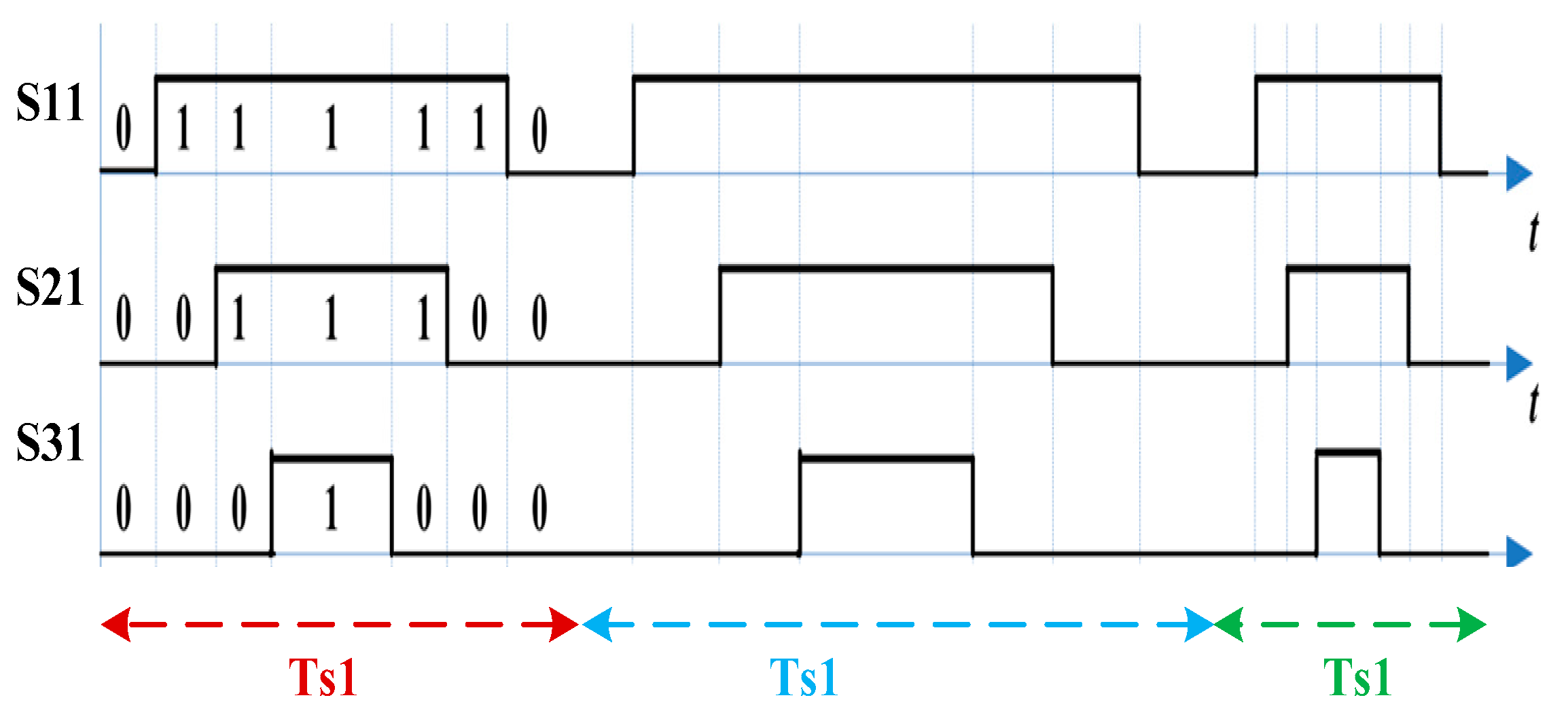
The RSF_SVPWM exploits the possibility of randomly changing period T of the switching signal and keeping the duty cycle and the delay report. Yet, for this algorithm, the triangular carrier wave is randomly changed. Since Fs = 1/Ts, the random change can be completed by changing the time of the triangular carrier. For sector 1, the signal generation mode of the RSF_SVPWM control is represented in Figure 9. In addition, when the timer period count value is randomly changed, the different switching cycles Ts1, Ts2, and Ts3 change to make the random adjustment of the switching frequency.

The limit of the variation interval of period T is given as follows:

$$\mathrm{T}\in \left[\overline{\mathrm{T}}\left(1-{\displaystyle \frac{{\mathrm{R}}_{\mathrm{T}}}{2}}\right),\overline{\mathrm{T}}\left(1+{\displaystyle \frac{{\mathrm{R}}_{\mathrm{T}}}{2}}\right)\right]$$

(13)

where $\overline{\mathrm{T}}$ is the statistical mean of the randomized period T, and R_T is the randomness level. Actually, R_T determines the interval in which T is randomized. The minimum value of the randomness level is theoretically (R_T)_min = 0, and the maximum value is (R_T)_max = 2, so the variation interval of the period is randomized between 0 and $2\overline{\mathrm{T}}.$ As a result, the instantaneous switching period T is expressed by

T = T_min + (T_max − T_min) × R

(14)

The T_min and T_max terms can be explained as follows:

$${\mathrm{T}}_{\min }=\overline{\mathrm{T}}\left(1-{\displaystyle \frac{{\mathrm{R}}_{\mathrm{T}}}{2}}\right)$$

(15)

$${\mathrm{T}}_{\max }=\overline{\mathrm{T}}\left(1+{\displaystyle \frac{{\mathrm{R}}_{\mathrm{T}}}{2}}\right)$$

(16)

Replacing T_max and T_min by their values in Equation (14), we obtain

$$\mathrm{T}={\mathrm{T}}_{\min }+\overline{\mathrm{T}}\times {\mathrm{R}}_{\mathrm{T}}\times \mathrm{R}$$

(17)

where R is a series of uniformly distributed random numbers in interval [0, 1].

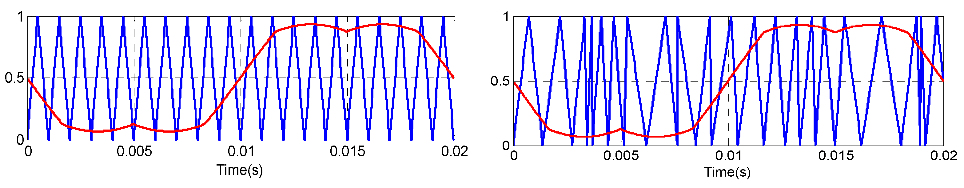
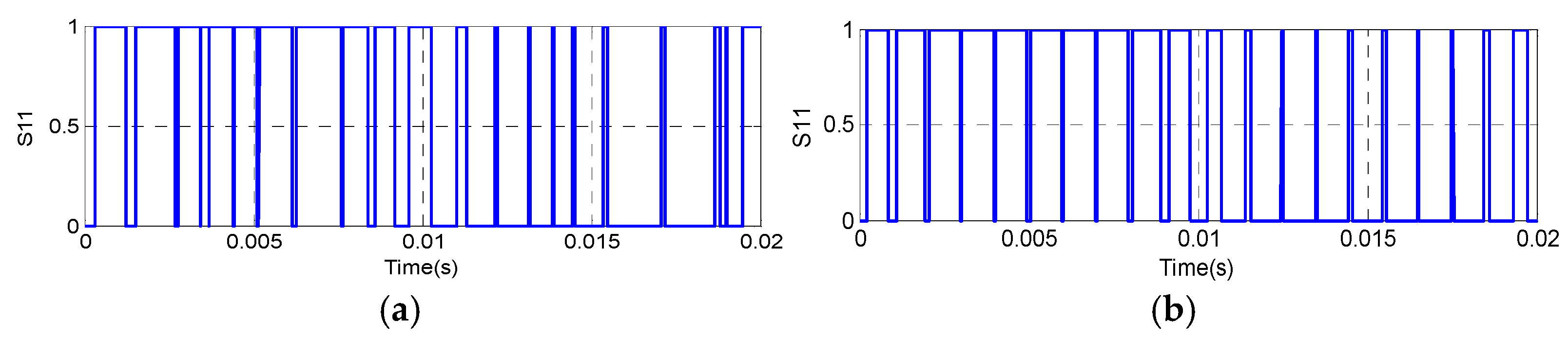
Therefore, Figure 10 depicts the waveforms of the random frequency carrier V_T, the modulation wave signal Vm and the switching sequence of switch S₁₁ for SVPWM and RSF_SVPWM control.

4. Simulation Analysis

A numerical simulation model of an IM fed by a two-level VSI controlled with SVPWM, RSF_SVPWM, RPP_SVPWM and RZV_SVPWM is developed and implemented on MATLAB/Simulink. In addition, the simulation results examine the characteristics of harmonic current spectra and the dynamic response of drives at different modulation indexes. The machine parameters are mentioned in

Table 1. The 0.5 Kw IM parameters.

Parameter	Value
Rated power	0.5 Kw
Motor speed	3000 tr/min
Stator resistance	24 Ω
Stator inductance	0.66 H
Rotor resistance	10.88 Ω
Rotor inductance	0.66H
Mutual inductance	0.63 H
Friction coefficient	0.00159
Inertia moment	0.004 Kg·m2
Pair pole number	1

. Simulation is performed under the same conditions: input voltage E = 560 V, switching frequency Fc = 5 kHz, and fundamental frequency F = 50 Hz. For all random SVPWM control, the uniform probability density function is used to perform all randomizations.

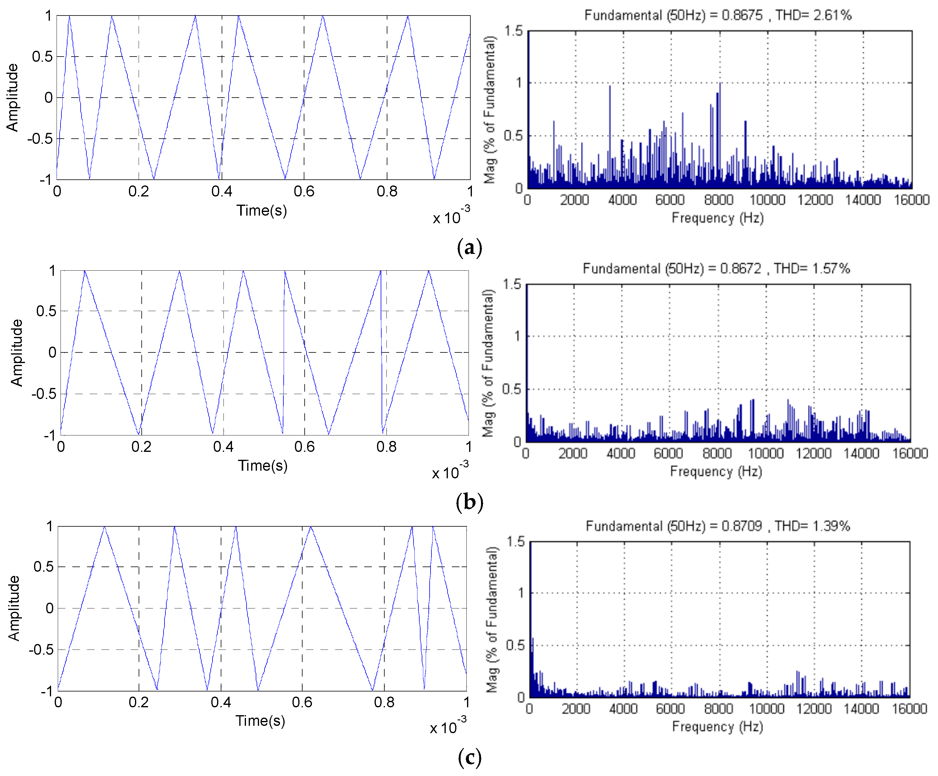
For the random RSFSVPWM control, randomness level RT plays a key role, since the distribution of harmonic spectra is affected by the parameters of the random triangular carrier. Accordingly, the RT parameter identifies the varying width of the PWM technique. The methodology to select the parameter of the triangular carrier is to make a sequence of simulation tests with different values of RT. Generally, in practice, randomness level RT does not generally exceed 0.5. We can note that if RT= 0, we have a constant switching frequency. In order to estimate the most appropriate RT parameter, a series of simulation tests are carried out to determine the Total Harmonic Distortion (THD) of the current corresponding to each R_T value. The results of the harmonic spectra of each randomness level signal (RT = 0.5, 0.3 and 0.1) are shown in Figure 11. For RT = 0.5, the triangular signal begins to vary randomly. In the same vein, we notice that the harmonic peak begins to attenuate with RT = 0.3. Furthermore, it is clear that RSF_SVPWM with RT = 0.1 provides a significant reduction in the THD value by 1.39% without neglecting the considerable reduction in the harmonic peak amplitude at the switching frequency and its multiples by spreading the energy spectrum over a wide frequency band. In this case, the results obtained from the RSF_SVPWM with a randomness level RT= 0.1 are more coherent and robust, and they significantly decrease the THD value compared to other cases.

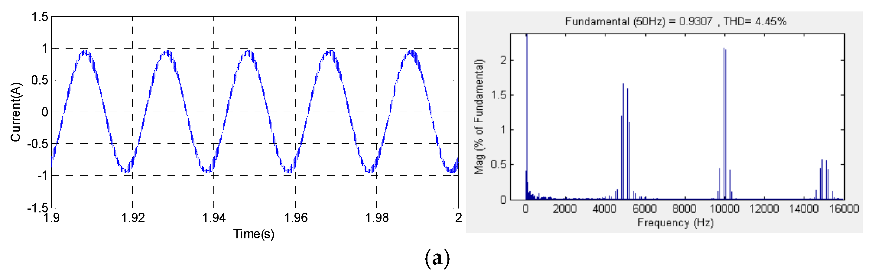
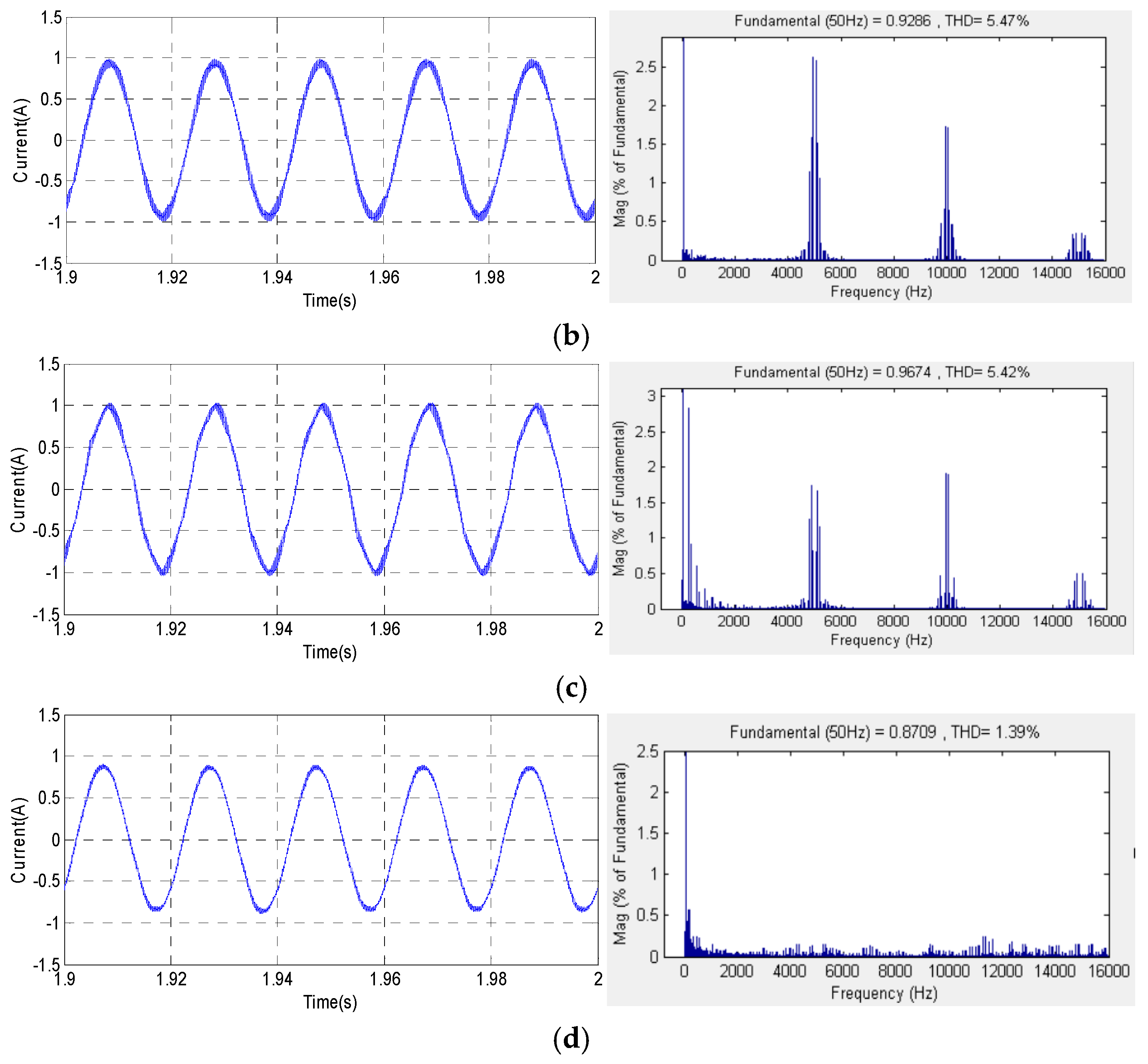
The acoustic PWM noise depends largely on the current noise. Figure 12 presents the stator current and its harmonic spectra waveforms, where im = 0.8 and Fc = 5 kHz, corresponding to SVPWM, RZV_SVPWM, RPP_SVPWM and RSF_SVPWM. The corresponding obtained THD values are 4.45%, 5.47%, 5.42% and 1.39%, respectively. Referring to the obtained results, it can be clearly noted that the high harmonic components are significantly generated by the SVPWM, RZV_SVPWM and RPP_SVPWM methods compared to the RSF_SVPWM. Therefore, the dominant magnitudes of the current harmonics are concentrated on the switching frequency and its multiples. In addition, the dominant harmonic magnitudes around the first switching frequency Fc are 1.66 A, 2.63 A and 1.74 A, respectively, for SVPWM, RZV_SVPWM and RPP_SVPWM. As a consequence, the harmonic magnitudes around the second switching frequency Fc are 2.17 A, 1.72 A and 1.92 A, respectively. However, for the RSF_SVPWM scheme, as depicted in the results given in Figure 12d, it is observed that there is a considerable reduction in the harmonic content. Nevertheless, the harmonic spectrum is totally spread better over the entire frequency band of the current, and the band around the switching frequency and its multiples disappear.

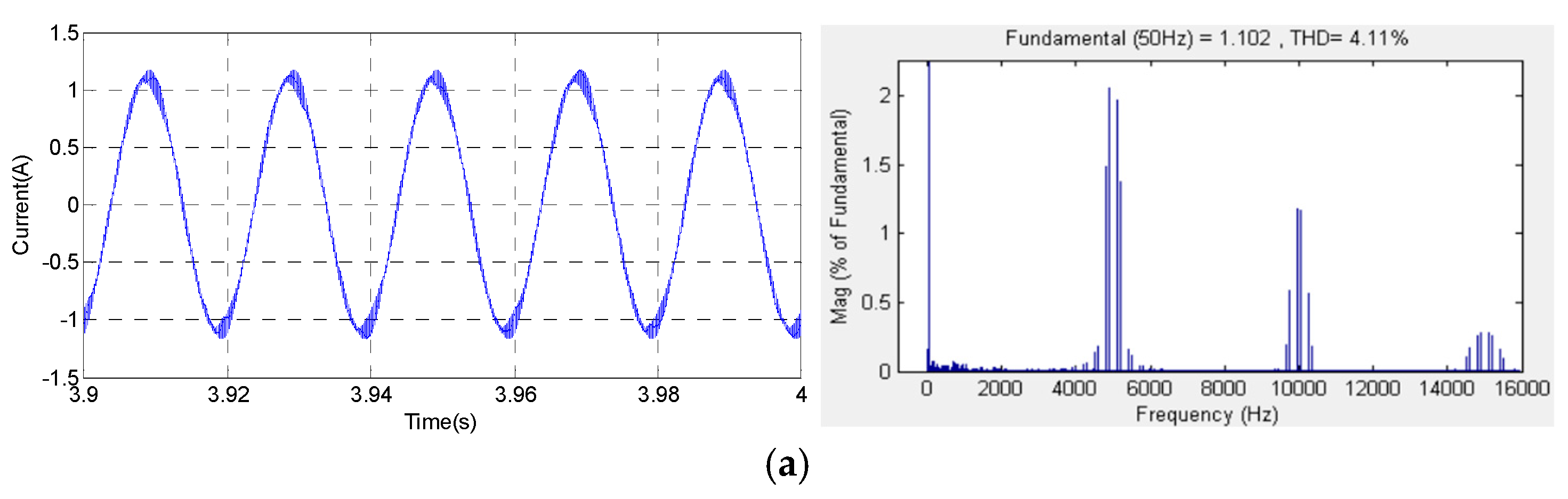
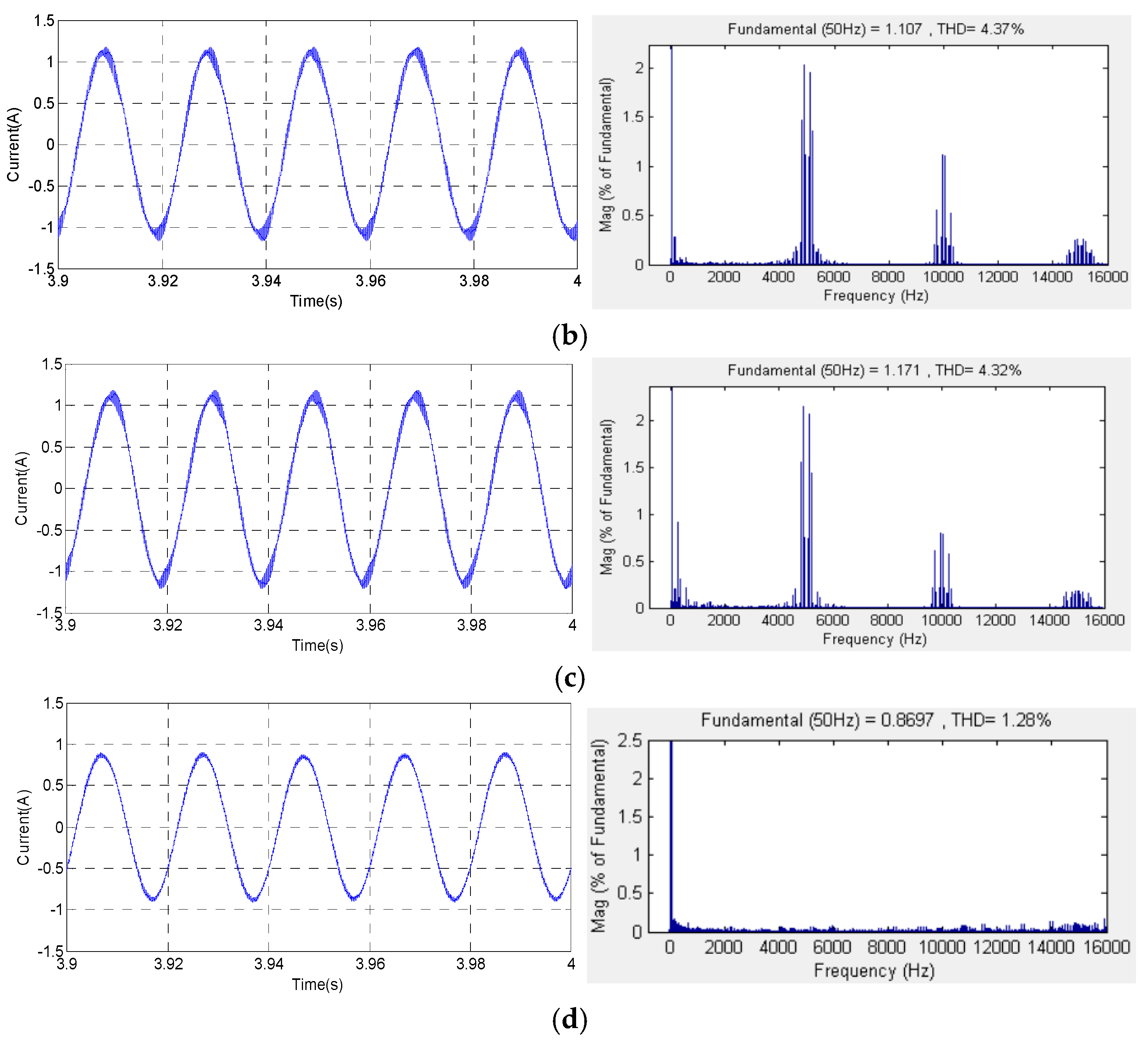
Figure 13 represents the waveforms of the stator current and the harmonic spectra corresponding to the proposed SVPWM, RZV_SVPWM, RPP_SVPWM and RSF_SVPWM strategies, where i_m = 1 and Fc = 5 kHz. Thus, the corresponding obtained THD values are 4.11%, 4.37%, 4.32% and 1.28%, respectively. In addition, it can be clearly noted that for all proposed strategies, the harmonic spectrum of the stator current is improved compared to i_m = 0.8. Furthermore, for the SVPWM, RZV_SVPWM, RPP_SVPWM strategies, the dominant harmonic is located around the switching frequency and its multiples. The important harmonic appears around the first switching frequency. In addition, the dominant harmonic magnitudes around Fc are 2.06 A, 2.03 A and 2.15 A, respectively. Thereby, the harmonic magnitudes around 2Fc are 1.18 A, 1.12 A and 0.8A, respectively. As shown by the simulation results, it is evidently noted that RSF_SVPWM control is the most effective in reducing and spreading the harmonic peaks over the entire frequency band, particularly at the first and second switching frequency Fc.

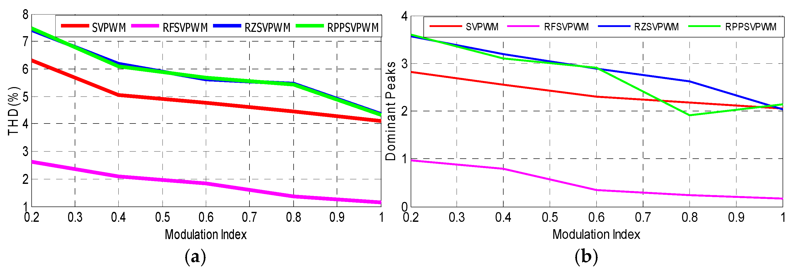
Next, the four proposed PWM control methods are examined in terms of THD current and dominant harmonic peaks. Figure 14 represents the variation according to the modulation index of the THD current and the harmonic peaks. It can be seen also that the obtained results are influenced by the values of the modulation index. As illustrated in Figure 14a, it is clearly seen that when the modulation index value increases, the THD level falls for all control. Added to that, the current harmonic content of RSF_SVPWM is significantly reduced and lower compared to other schemes. The fixed SVPWM produces a lower THD compared to the RZV_SVPWM and RPP_SVPWM control. Hence, as shown in Figure 14b, the magnitude of the current harmonic is reduced significantly for RSF_SVPWM over the entire modulation range compared to other schemes. In conclusion, RSF_SVPWM is the most effective in reducing the THD current and spreading the harmonic spectra compared to the fixed SVPWM scheme, RZV_SVPWM and RPP_SVPWM.

The impact of the proposed techniques is demonstrated and verified on a 1.5 kW motor. The electrical and mechanical characteristics and parameters of this machine are provided in

Table 2. The 1.5 Kw IM parameters.

Parameter	Value
Rated power	1.5 Kw
Motor speed	1435 rpm
Stator resistance	5.72 Ω
Stator inductance	0.464 H
Rotor resistance	4.28 Ω
Rotor inductance	0.464 H
Mutual inductance	0.44 H
Friction coefficient	0.002
Inertia moment	0.0049 Kg·m2
Pair pole number	2

. Simulation is performed under the same conditions on a 0.5 kW motor: input voltage E = 560 V, switching frequency Fc = 5 kHz, and fundamental frequency F = 50 Hz. A numerical simulation model of an IM fed by a two-level VSI controlled by SVPWM, RSF_SVPWM, RPP_SVPWM and RZV_SVPWM is developed and implemented on MATLAB/Simulink. Moreover, the simulation results examine the characteristics of the harmonic current spectra and the dynamic response.

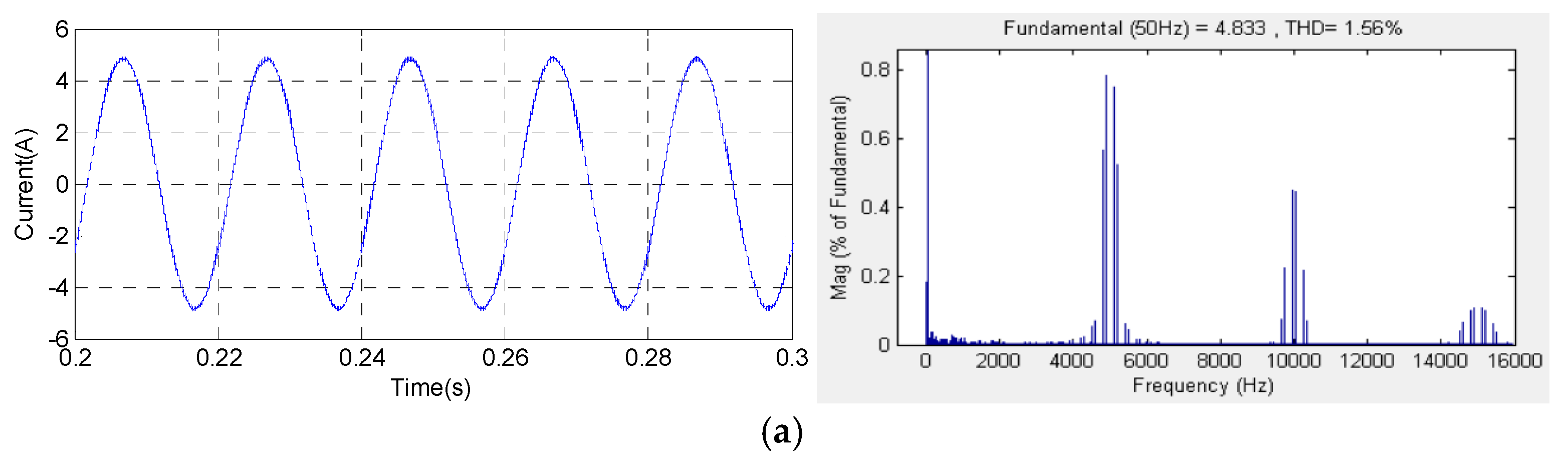
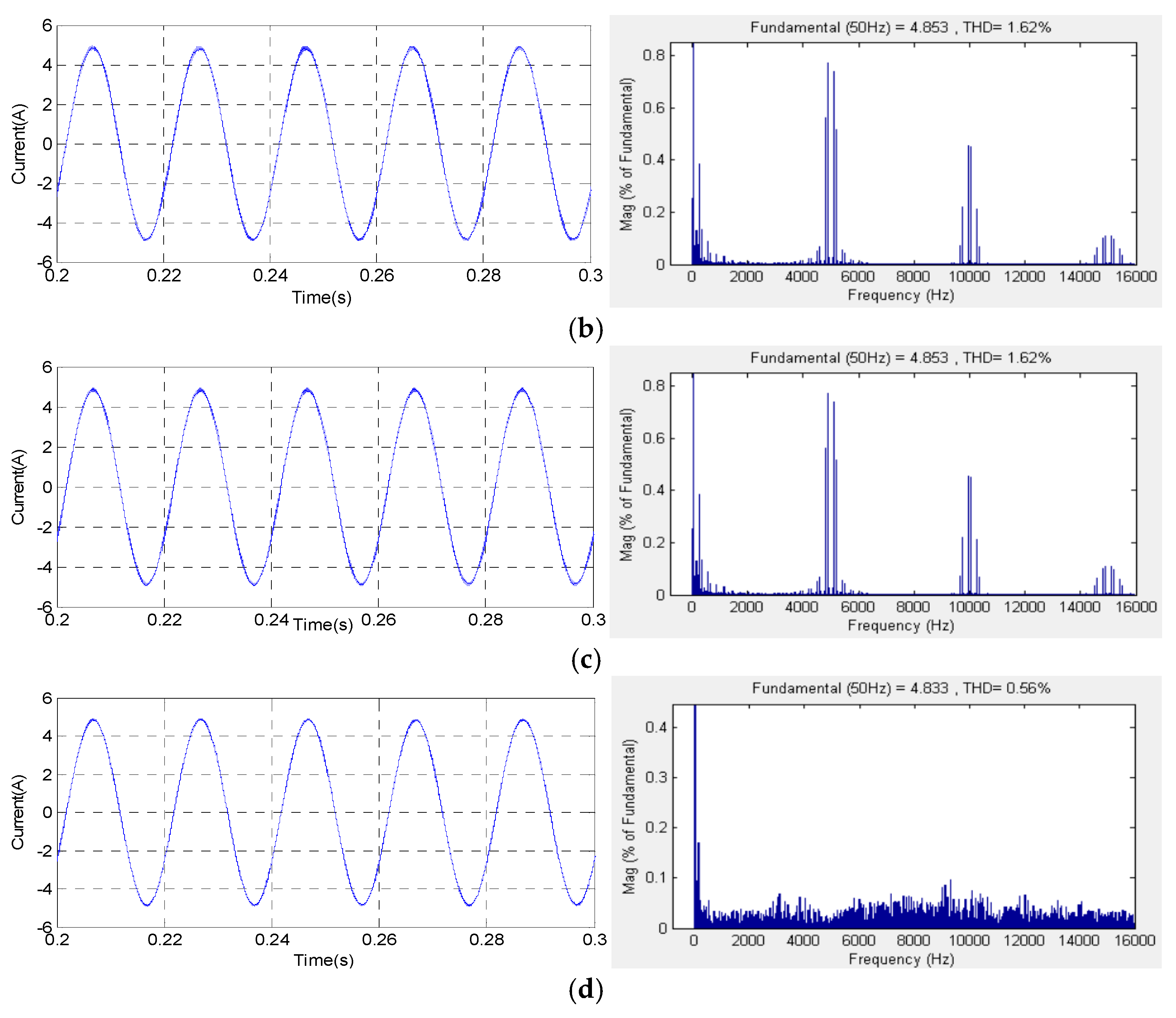
The acoustic PWM noise depends largely on the current noise. Figure 15 presents the stator current and its harmonic spectra waveforms, where im = 1 and Fc =5 kHz, corresponding to the studied SVPWM, RZV_SVPWM, RPP_SVPWM and RSF_SVPWM techniques. The obtained THD values are 1.56%, 1.71%, 1.62% and 0.56%, respectively. Referring to the obtained results, it can be clearly noted that the high harmonic components are significantly generated by the SVPWM, RZV_SVPWM and RPP_SVPWM methods, compared to RSF_SVPWM, on a 1.5 kW motor. Hence, the dominant magnitudes of the current harmonics are concentrated on the switching frequency and its multiples for SVPWM, RZV_SVPWM and RPP_SVPWM. However, for RSF_SVPWM, it is observed that there is a considerable reduction in the harmonic content. However, the harmonic spectrum is totally spread better over the entire frequency band of the current, and the band around the switching frequency and its multiples disappear. In conclusion, we have verified by simulation results through harmonic analysis that the effect of the studied techniques has the same impact for the two motor types. Additionally, on a 0.5 kW motor, the harmonic level is high compared to the 1.5 kW motor. Then, the current’s harmonic spectrum is reduced for the RSF_SVPWM technique for both motors.

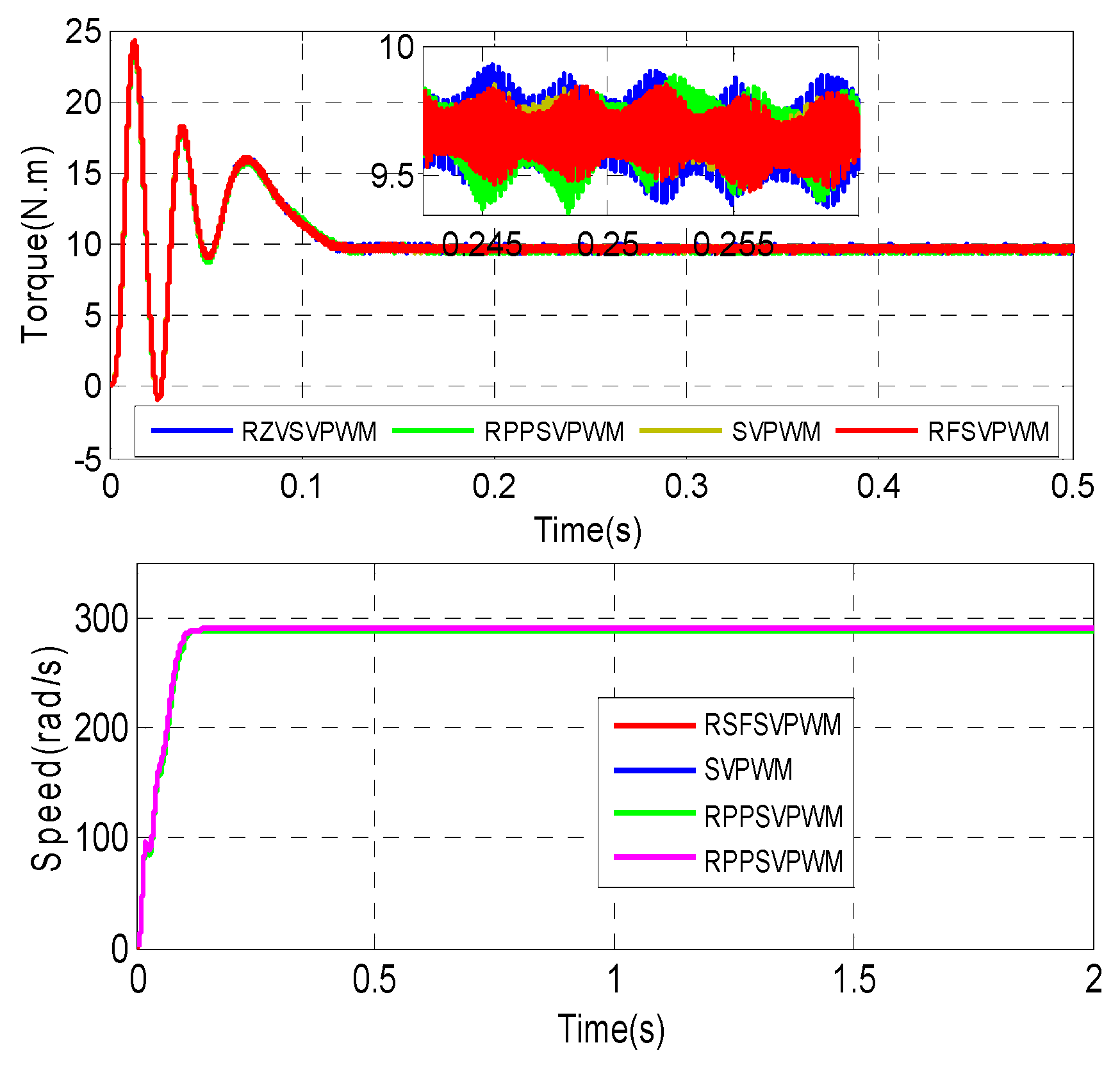
The temporal waveform evolution of the electromagnetic torque and speed for the studied SVPWM, RZV_SVPWM, RPP_SVPWM and RSF_SVPWM techniques, where Fc = 5 kHz and Im = 1, is presented in Figure 16. The steady state is established after 0.15 s for the four techniques. Thus, a high oscillation is generated with RZV_SVPWM and RPPSVPWM, but the RSFSVPWM method also ensures a better response. The motor speed oscillates for the first few moments, and then it stabilizes around a nominal value.

5. Experimental Results

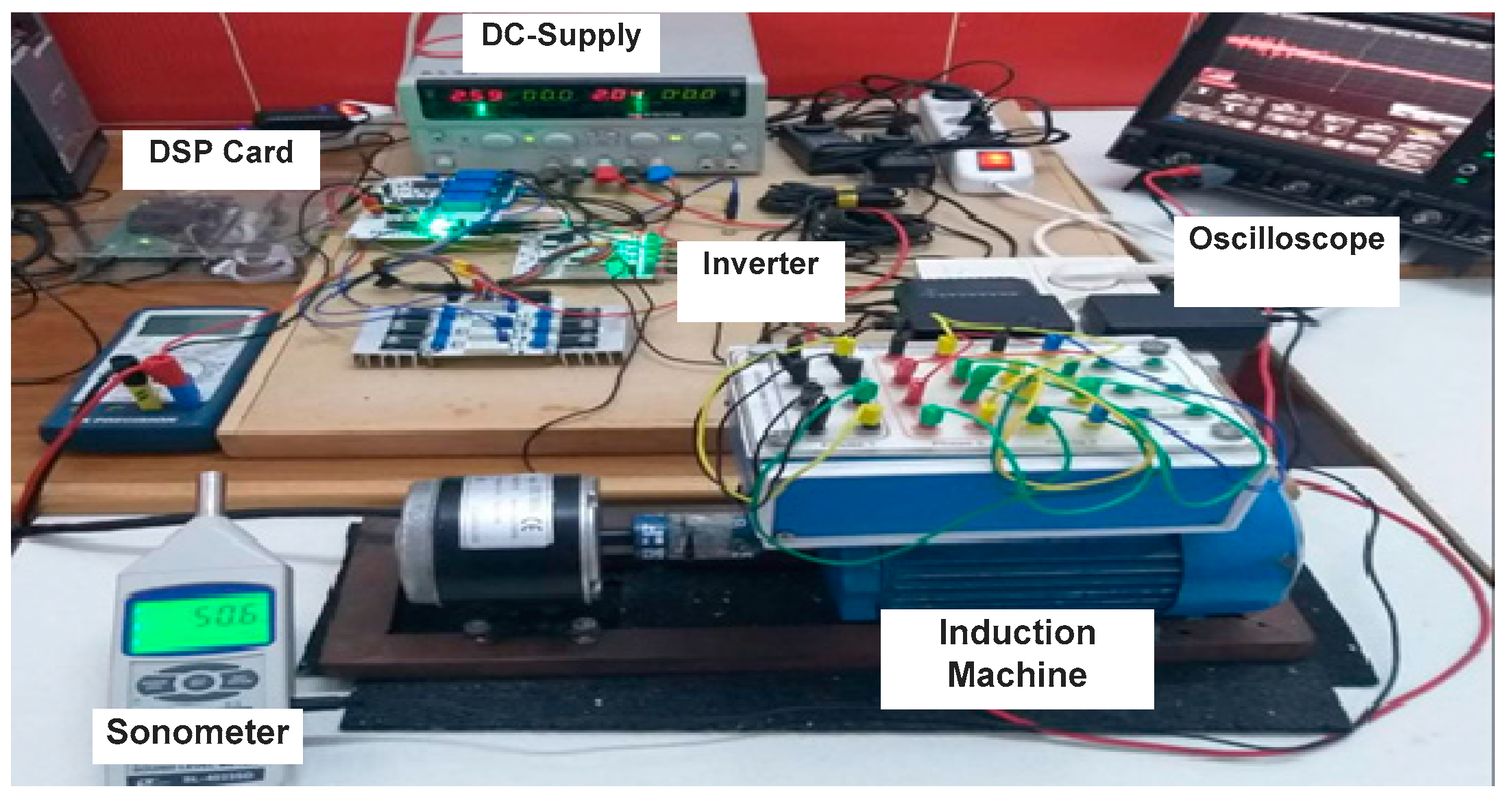
The photo of the experimental system for acoustic noise measurements is depicted in Figure 17. It consists mainly of an IM, a DSP board and a two-level VSI controlled by SVPWM, RZV_SVPWM, RPP_SVPWM and RSF_SVPWM. We have implemented all the proposed strategies using the TMS320F28335 DSP board from Texas Instruments. The motor runs at a fundamental frequency of F = 50 Hz and a switching frequency of Fc = 5 kHz. A sound level meter is used to measure the instantaneous sound pressure. After each measurement test, the saved data file is transferred to the PC. The spectral noise analysis is performed using MATLAB’s FFT function. The machine used in this study is classified as a small machine. Therefore, all measurement points must be located at a 250 mm distance or more from the main machine surface. Measurements should be carried out when the machine reaches a steady state of the operating mode [8,22,23,24].

The sound pressure level in decibels (dB) can be described using the sound pressure, which is determined by Equation (18):

$${\mathrm{L}}_{\mathrm{p}}(\mathrm{t})=20{\log }_{10}\left({\displaystyle \frac{\mathrm{p}(\mathrm{t})}{{\mathrm{p}}_0}}\right)$$

(18)

where p₀ is the reference sound pressure, and p(t) is the instantaneous sound.

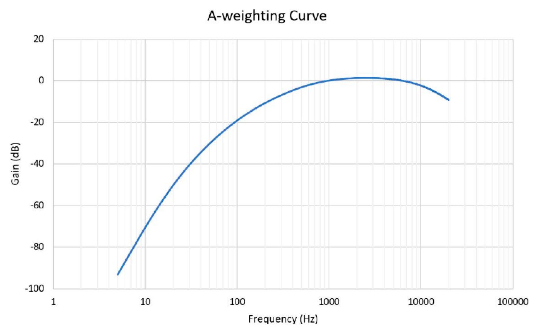
The human ear sensitivity can be modeled using appropriate weighting functions or curves. International standards recommend weighting curves. The A-weighting curve is widely used in electrical machine acoustics and is also utilized in this work. Figure 18 illustrates the dB(A) weighting curve according to IEC 61672-1/2002 [22].

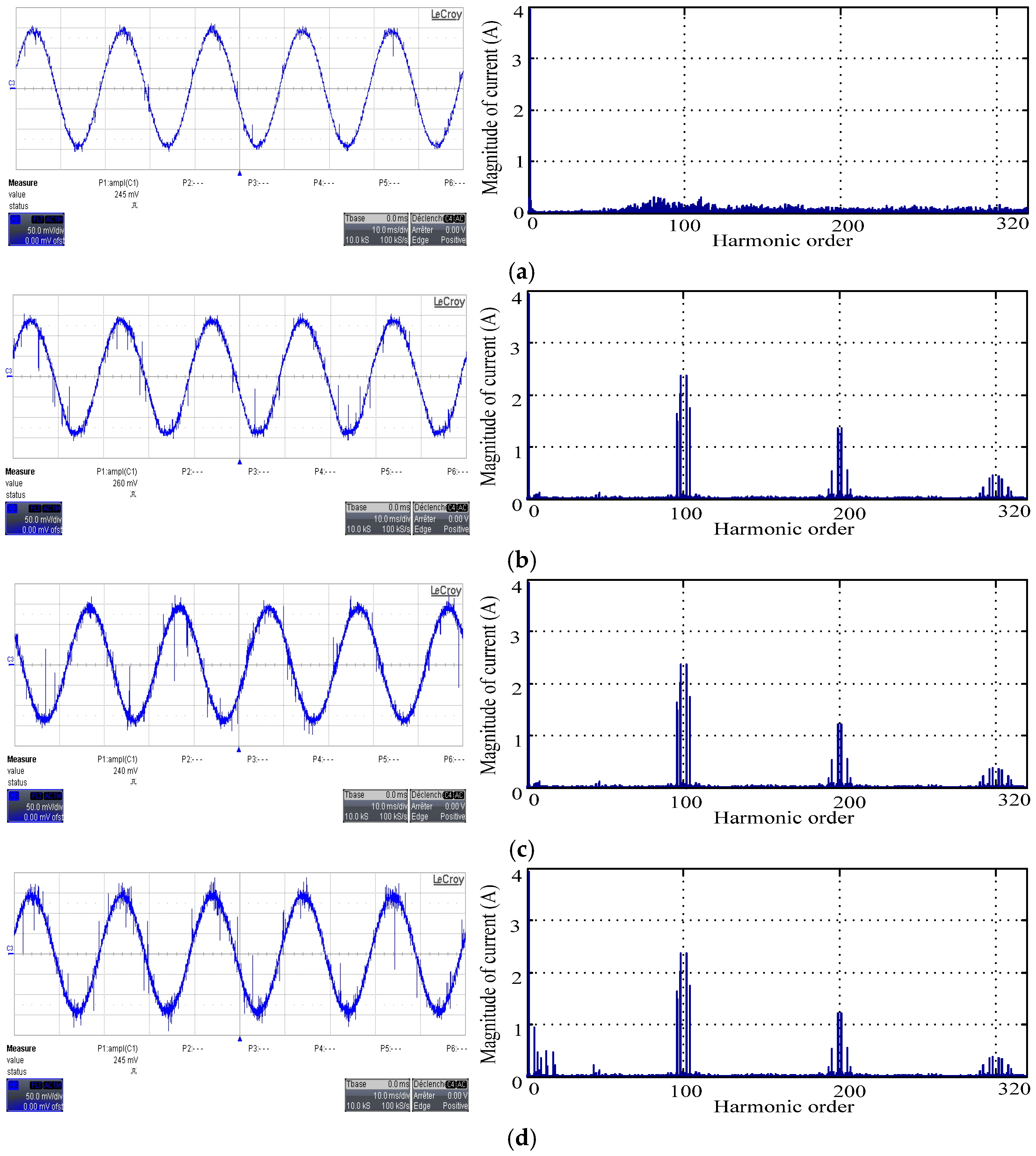
The measured stator current waveforms and the harmonic spectrum produced by the IM supply by a two-level VSI and are controlled by the SVPWM, RZV_SVPWM, RPP_SVPWM and RSF_SVPWM techniques, where im = 1 and Fc = 5 KH are represented in Figure 19. As it can be seen from the results of the measured harmonic spectrum, with the SVPWM, RZV_SVPWM and RPP_SVPWM techniques, the dominant harmonics components are concentrated around the switching frequency and its multiples. Furthermore, the highest magnitudes of current harmonics are located around the first sideband of the switching frequency. However, it can be observed that the magnitude of current harmonics is reduced considerably with RSF_SVPWM compared to the other strategies. Furthermore, the motor current spectrum is well dispersed, and the harmonics around integer multiples of the switching frequency disappear. As a consequence, it is evident that the proposed RSF_SVPWM scheme has better performance in terms of acoustic noise, as it will be seen in the next section.

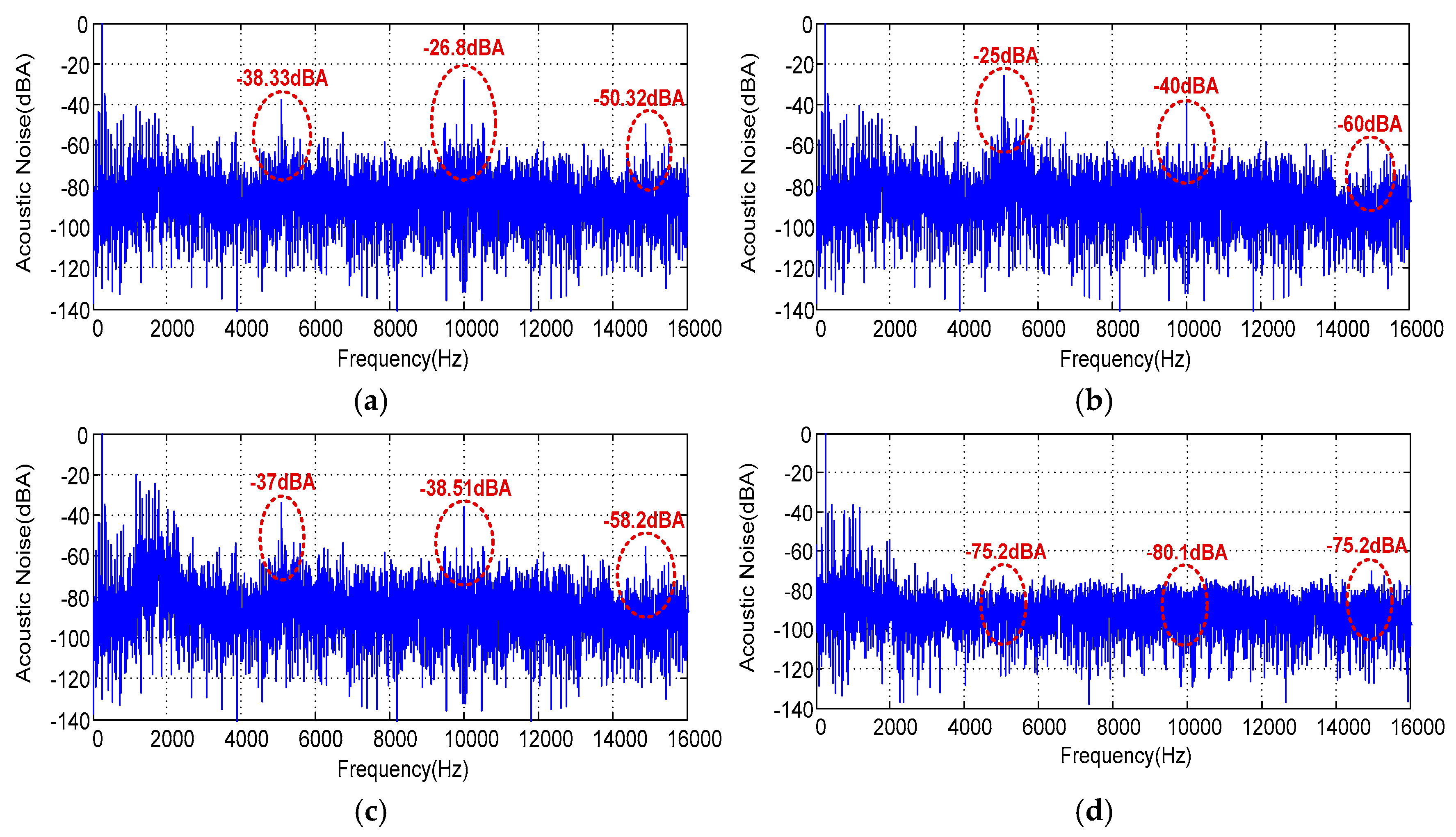
The weighted frequency spectra of acoustic noise corresponding to the SVPWM, RZV_SVPWM, RPP_SVPWM and RSF_SVPWM techniques, where im = 0.8 and Fc = 5 kHz and where im = 1 and Fc = 5 kHz, are performed and demonstrated, respectively, in Figure 20 and Figure 21. Referring to the experimental results, we can observe that the acoustic noise emitted from the IM is generated with SVPWM, RZV_SVPWM and RPP_SVPWM. The high acoustic noise components are significant around integer multiples of the switching frequency, as shown in Figure 20a–c. The dominant noise of these techniques is mainly due to the interaction of the switching frequency and the higher time harmonics. When im = 0.8, the noise amplitude is −38.33 dBA, −26.8 dBA and −50.32 dBA for SVPWM, −25 dBA, −40 dBA and −60 dBA for RZV_SVPWM and −37 dBA, −38.51 dBA and −58.2 dBA for RPP_SVPWM, respectively, at 5, 10 and 15 KHz. However, for the RSF_SVPWM technique, the dominant noise components emitted from the IM around the integer multiples of the switching frequency disappear and the spectrum is spread, as presented in Figure 20d. It is clearly noticed that RSF_SVPWM produces a less noisy component than the other techniques. The noise amplitude is −75.2 dBA, −80.1 dBA and −75.2 dBA, respectively, at 5Khz, 10 kHz and 15 kHz. These results confirm the effectiveness of the proposed RSF_SVPWM scheme in reducing the acoustic noise emitted by the IM.

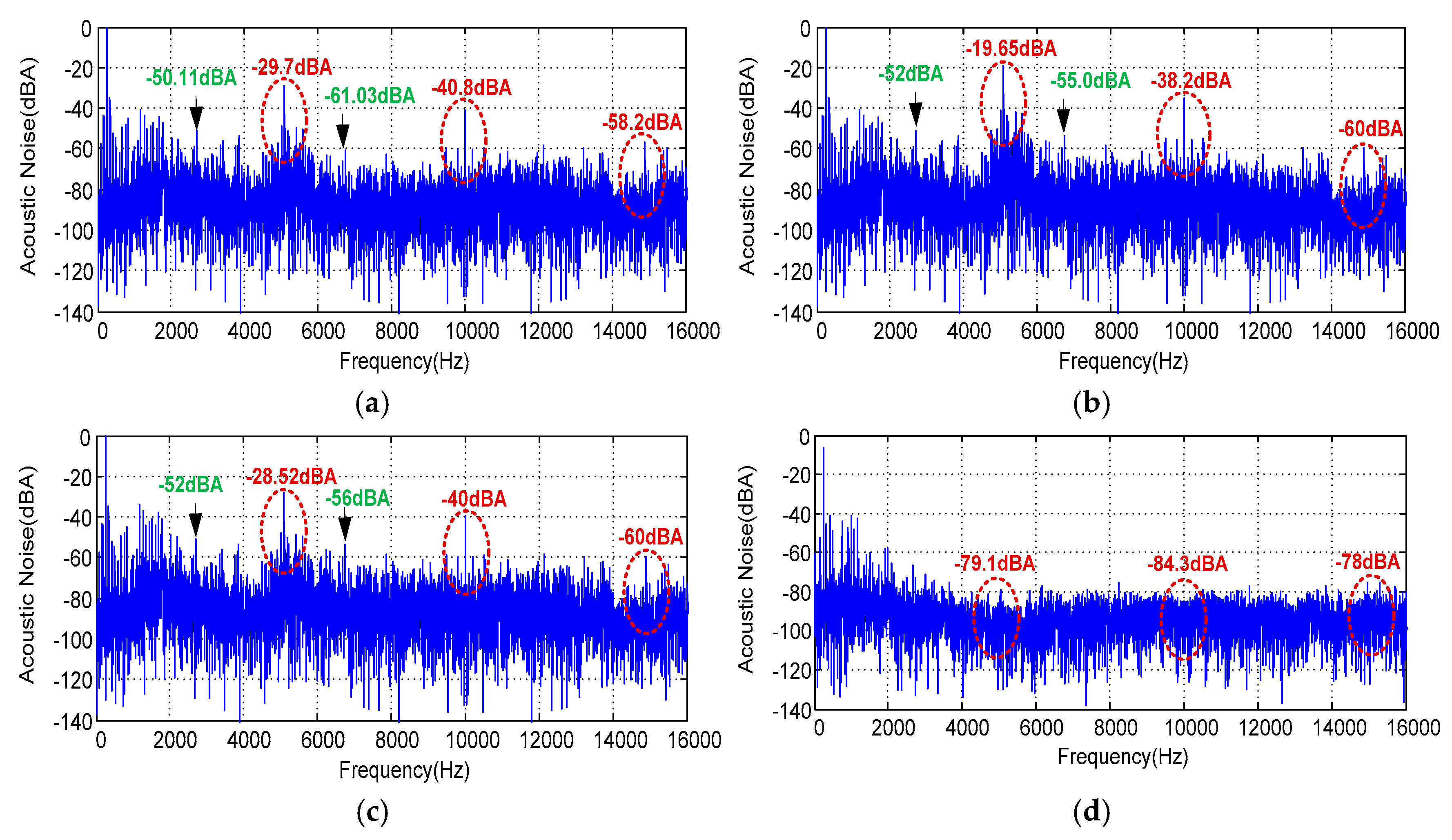
The measured acoustic noise spectra where i_m = 1 and Fc = 5 kHz are presented in Figure 21. The same observations are valid in Figure 21d, where the acoustic noise emitted from the IM is totally spread for the RSF_SVPWM technique. In addition, for index modulation i_m = 1, the acoustic noise falls down for the four proposed PWM techniques. Accordingly, the noise amplitude is −29.7 dBA, −40.8 dBA and −58.2 dBA for SVPWM, −19.65 dBA, −38.2 dBA and −60 dBA for RZV_SVPWM, −28.52 dBA, −40 dBA and −60 dBA for RPP_SVPWM and −79.1 dBA, −84.3 dBA and −78 dBA for RSF_SVPWM, respectively, at 5, 10 and 15 kHz. Generally, the mechanical behavior of the stator can be characterized by its natural modes of vibration. Each mode, corresponding to a proper frequency, represents a particular deformation of the structure. The main modes of the stator deformation are shown in Figure 3. The proper frequencies for a 0.5 kW IM for this study with 17 rotor bars, 24 stator slots and 1 pole pair for different modes (0, 1, 2, 3, 4, 5) are, respectively, 14,033, 19,845, 2878, 7624, 13,461 and 19,922 Hz. Consequently, the generation of the magnetic forces on different frequencies near to the machine’s natural frequency leads the machine to vibrate and produces a higher level of noise. Generally, the noise magnitude can increase due to the resonance phenomena. For example, when im = 1 and Fc = 5 kHz, and with SVPWM at frequencies 2400 Hz and 6450 Hz close to 2878 Hz and 7624 Hz for vibrational modes m = 2 and m = 3, the levels of acoustic noise are, respectively, equal to −50.11 dBA and −61.03 dBA. In addition, with RZV_SVPWM, for vibrational modes m = 2 and m = 3, at frequencies 2400 Hz and 6450 Hz, the levels of acoustic noise are, respectively, equal to −52 dBA and −55.0 dBA. Therefore, with RPP_SVPWM, the noise at 2878 Hz is equal to −50 dBA, and at 8562 Hz, it is equal to −56 dBA. In conclusion, the obtained results show that the noise magnitude is uniformly reduced with RSF_SVPWM.

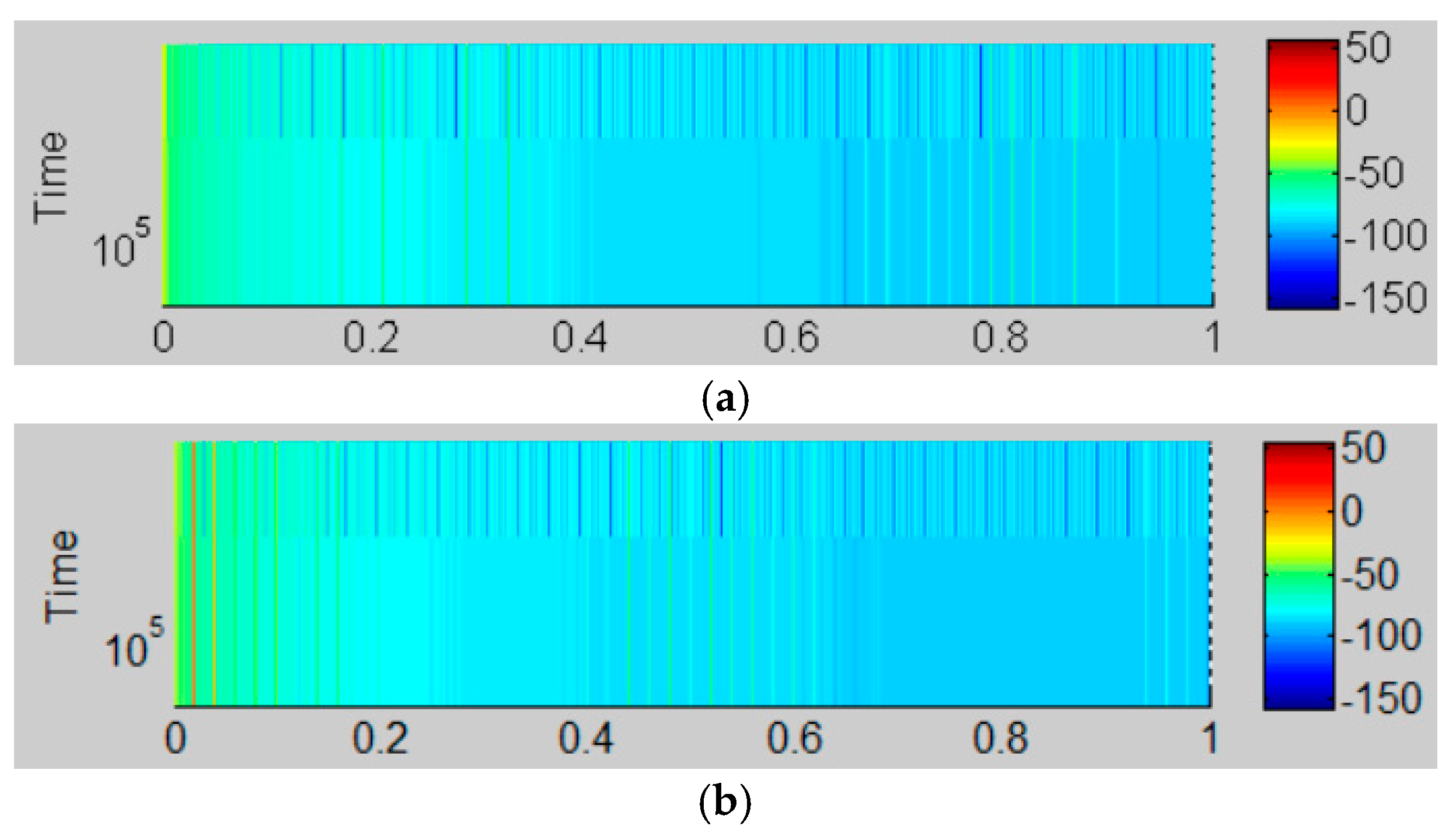
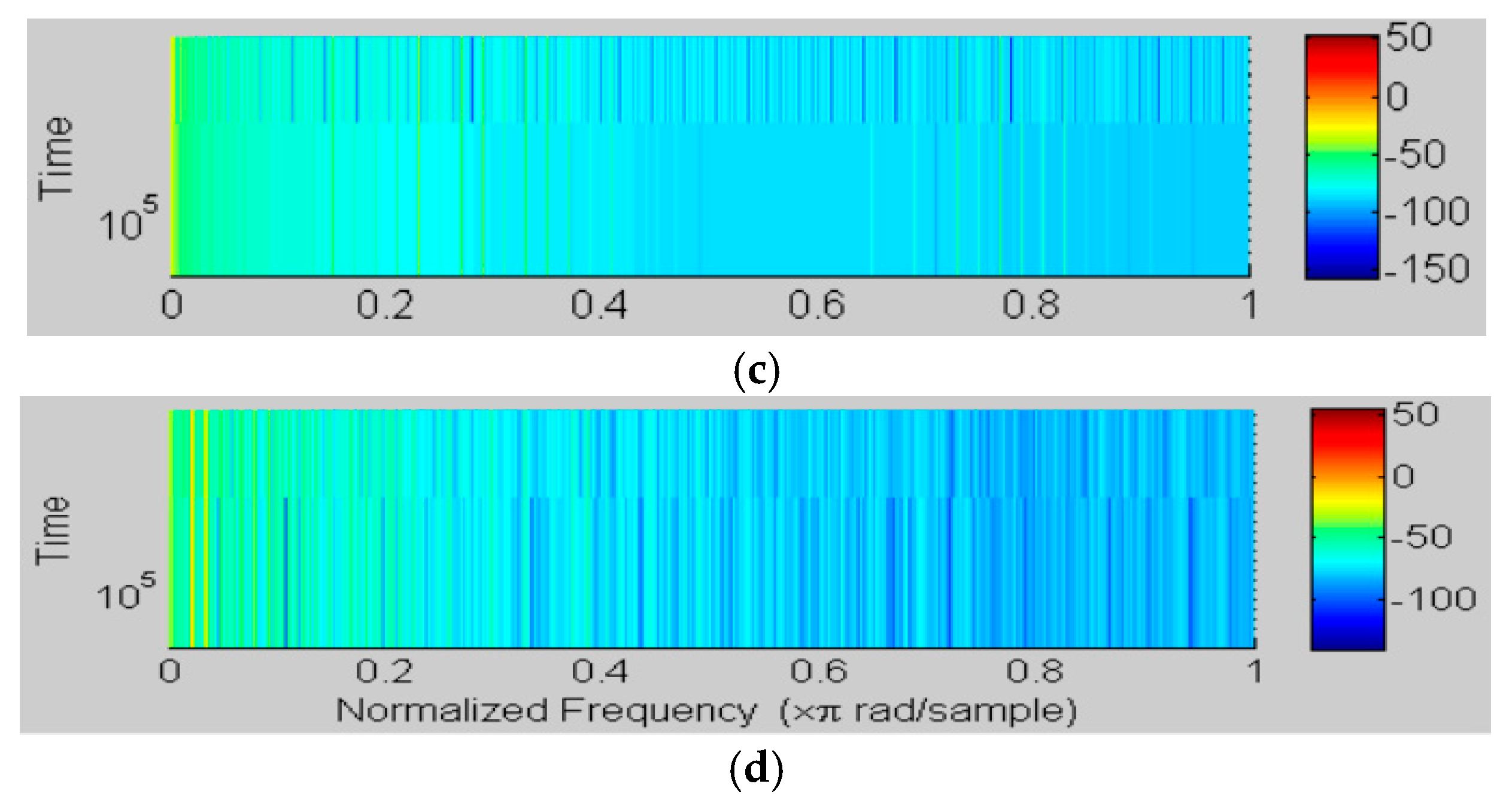
Figure 22 presents the time–frequency spectra corresponding, respectively, to the studied techniques where im = 1 and Fc = 5 kHz. These results show that SVPWM, RZV_SVPWM and RPP_SVPWM give practically the same characteristics in terms of current spectrogram. Moreover, RSFSVPWM gives better performance.

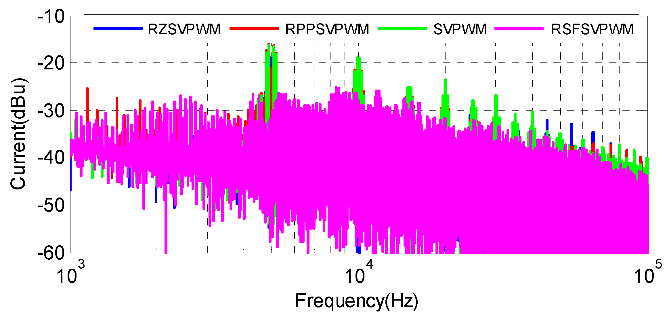
The current frequency spectra corresponding to the studied techniques are depicted in Figure 23. The SVPWM, RZV_SVPWM and RPP_SVPWM methods generate the most significant harmonics with the highest at 5 kHz and its multiples. With RSFSVPWM, on the other hand, the spectrum is totally dispersed over the entire frequency band. Thus, according to the similarity of the numerical and experimental results, we can confirm that RSF_SVPWM is practically more adapted to minimize the harmonics of the current and the acoustic noise.

Table 3. Comparison of SVPWM, RPWM and RSF_SVPWM techniques.

	SVPWM	RPWM	RSF_SVPWM
THD current (%)	4.87	3.92	1.49
Acoustic noise (dBA)	−29.7	−59.79	−79.1
Frequency	Fixed	Random	Random

compares the SVPWM, RPWM and RSFSVPWM techniques in terms of current THD (%), and acoustic noise level (dBA) emitted by an IM. It should be remembered that for the RPWM technique developed in our previous study, the values for the current and the acoustic noise are 3.92% and −59.79 dBA, respectively. Therefore, it is noted that the RSF_SVPWM technique has a lower THD and acoustic noise level than fixed SVPWM and RPWM.

6. Conclusions

This paper has examined the impact of the random SVPWM control in terms of PWM acoustic noise emitted IM fed by a three-phase two-level VSI. In addition, fixed SVPWM, RSF_SVPWM, RZV_SVPWM and RPP_SVPWM have been proposed and investigated theoretically and experimentally. The simulation results of the harmonic current have demonstrated that with SVPWM, RPPSVPWM and RZVSVPWM, the harmonics components have been produced near the switching frequency and its multiples under different modulation indexes. Nevertheless, the harmonic spectrum of the suggested RSF_SVPWM has been totally spread over the entire frequency band, and the band around the switching frequency anhd its multiples have disappeared. The experimental validation of the studied control strategies has been evaluated using a lab prototype of an inverter-fed IM drive. The proposed RSF_SVPWM could able to provide good performance in terms of current quality (THD) and reduce the acoustic noise of VSI-fed motor drives compared to RZV_SVPWM and RPP_SVPWM as well as to fixed SVPWM.