2.1. Experiments in Structural Vibration Control
Experiments with TLDs are particularly important in the field of structural vibration control for several reasons. First, the behavior of TLDs is typically modeled using fluid dynamics and vibration theory. Second, TLDs often exhibit nonlinear behavior due to fluid sloshing, which can be difficult to predict accurately using purely analytical methods. Experiments help identify and account for these nonlinearities, improving control strategies and damper design [
14]. In addition, experimental studies allow engineers to optimize key parameters, such as the size, shape, and placement of TLDs, ensuring maximum vibration suppression for specific structures. These experiments help refine the design to achieve greater efficiency [
15]. Furthermore, experiments replicate real-world conditions (such as wind, earthquakes, and other dynamic forces), helping to assess how TLDs perform under actual loading scenarios. This is critical for ensuring safety and stability in applications like tall buildings or bridges [
16]. Testing new technologies, like the integration of MRFs in TLDs, requires experiments to validate how these innovations enhance performance, offering active or semi-active control of vibrations [
17].
Escalante–Martínez et al. [
18] proposed an experimental design to analyze the viscous damping coefficient in a mass/spring/damper system using different fluids such as water, edible oil, and motor oil. By observing the free decay of a mass submerged in the fluids, the logarithmic decrement of the response is measured, allowing for the determination of the damping coefficient. Their findings confirm that the damping coefficient increases with fluid viscosity, demonstrating a clear relationship between viscosity and energy dissipation. The inclusion of vegetable-based oil aims to evaluate its performance as an alternative to petroleum-derived lubricants due to its renewable nature and high biodegradability, which make it a promising option in sustainable engineering applications.
To investigate the impact of magnetic fields on the fluid viscosity and, consequently, on its damping, a uniform and controlled magnetic field is required. The Helmholtz coil is a pair of identical coils placed symmetrically and separated by a distance equal to the radius of the coils. This specific arrangement, in which the current flows in the same direction on both coils, produces a nearly uniform magnetic field in the region between the coils, making them ideal for practical experimentation and analysis. This principle relies on the Biot–Savart law and the superposition of magnetic fields [
19].
The viscosity of ferromagnetic fluids varies with the strength and orientation of an applied magnetic field, depending on the ratio of hydrodynamic stress to magnetic stress [
20]. For low ratios, viscosity is field-dependent, while at high field values, it becomes field-independent. Ohno et al. [
21] devised a cylindrical container-tuned magnetic fluid damper and studied the effects of varying the depth of the magnetic fluid and the applied magnetic field on the damper’s performance. It was found that the presence of magnetic fluid significantly suppresses vibrations, especially near the natural frequency of the structure.
2.2. Measurement of Viscosity
The viscosity of a fluid can be measured through the falling-sphere method, where a sphere of known size and density is dropped into a fluid [
22]. The motion of a sphere falling through a viscous fluid in a tube is governed by several forces, primarily gravity, buoyancy, and viscous drag [
23]. The forces acting on a sphere of radius
r are depicted in
Figure 1. The dynamics are described using Stokes’ law and the equations of motion for the sphere. It must be noted that for the description of the system, laminar flow, isotropic and Newtonian fluid with constant properties is assumed. Given the experimental approach conducted in this work, it is worthwhile mentioning that classical Stokes laws do not account for potential nonlinear effects that may arise at high concentrations of the ferromagnetic particles included in the carrier fluids, or anisotropies in the magnetic field applied. Therefore, the validity of these equations is primarily limited to conditions where the concentration of ferromagnetic particles is low enough to minimize collective interactions and nonlinear effects and when the applied magnetic field remains uniform.
The gravitational force acting on the sphere is given by:
where
is the volume of the sphere,
is the density of the sphere, and
is the acceleration due to gravity. The volume of the sphere is calculated according to the equation:
The buoyant force is the upward force exerted by a fluid on an object that is either partially or fully submerged in it. This force occurs because of the pressure difference between the top and bottom of the object caused by the fluid’s weight. It is given by the equation:
where
is the density of the fluid.
The viscous drag force is the resistive force exerted by the fluid on the sphere moving through it. This force is a result of the viscosity of the fluid, which is a measure of its resistance to flow or deformation. The viscous drag opposes the motion of the object and increases with the object’s speed and the fluid’s viscosity. For low Reynolds numbers (
), the viscous drag of a sphere submerged in the fluid is given by Stokes’ law:
where
is the dynamic viscosity of the fluid, and
is the velocity of the sphere. The viscosity of a fluid can be experimentally determined [
23].
The equation of motion of the sphere is governed by the net force acting on it, which, in turn, determines its acceleration.
The sphere submerged in a viscous fluid reaches a terminal velocity, which is the constant speed it achieves when the net force acting on it is zero and, therefore, the acceleration equals zero. This occurs when the downward gravitational force is exactly balanced by the upward buoyant force and the resistive viscous drag force:
This equation shows that the terminal velocity increases with the square of the radius of the sphere, with the difference in density between the sphere and the fluid and with the inverse of the viscosity of the fluid.
Before reaching terminal velocity, the motion can be described by the following expression:
Substituting the term of the volume of the sphere, operating and simplifying further:
The term that accompanies the velocity
can be renamed as
. This is a first-order linear differential equation. Using an integrating factor or solving directly, the velocity
is:
where
is the initial speed. Ideally, the sphere approaches the terminal velocity asymptotically rather than reaching it exactly in finite time. This behavior arises from the exponential term in the velocity equation over time.
From this expression it can be derived that whether the body immersed in the fluid is in force equilibrium or subjected to a non-zero force resulting, the viscosity of the fluid is lower and the faster the movement. Altering the viscosity of the fluid at will would create an effective damper to cope with the vibrations to which a structure may be subjected. Therefore, the activation of a magnetic field is a strategy of great interest in the design of vibration control systems.
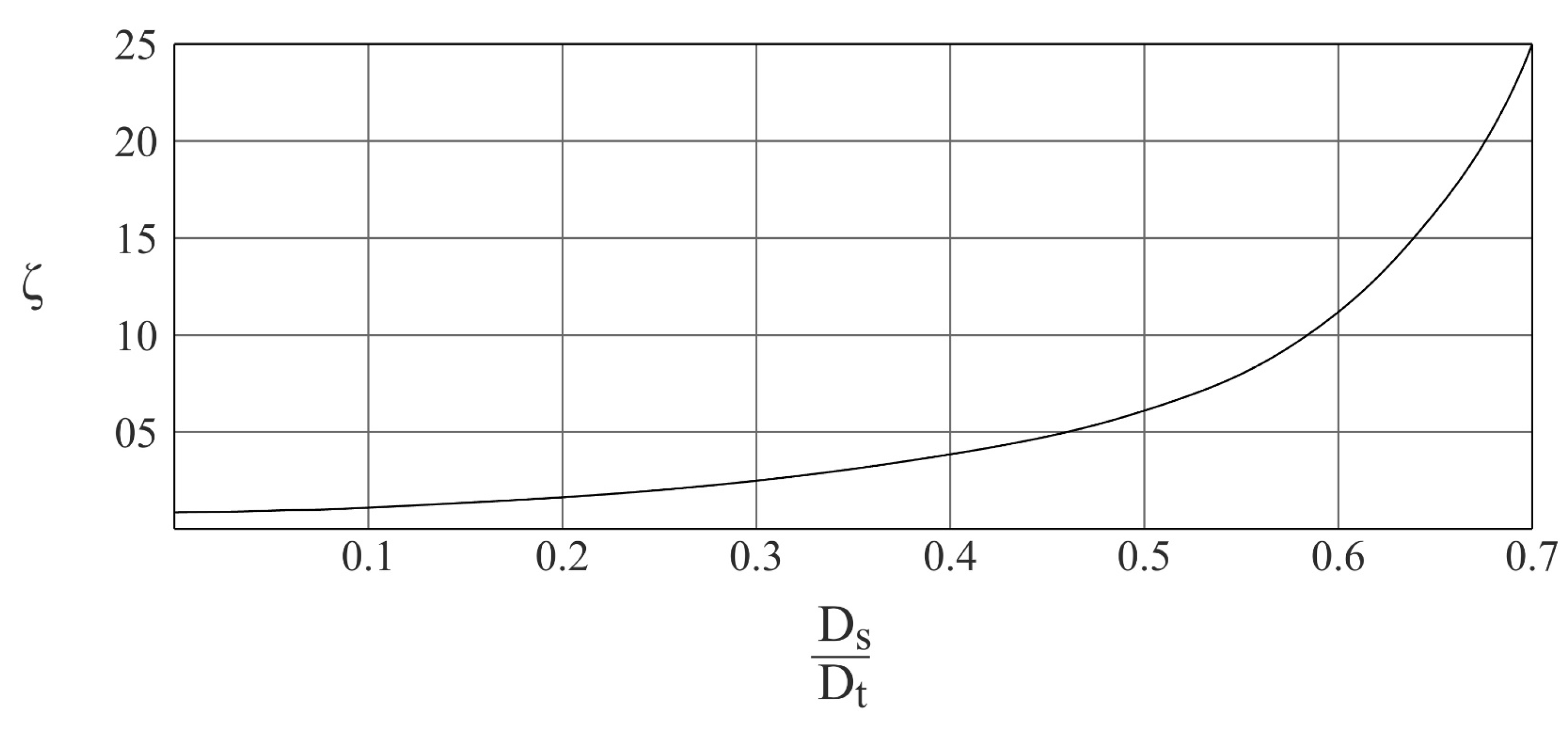
It must be noted that this procedure considers that the sphere has a low velocity profile and that its diameter is small with respect to the diameter of the tube, given by a value of the ratio in Equation (11) equal to or lower than 0.2.
where
corresponds to the diameter of the sphere and
represents the diameter of the tube. For greater ratios, a correction factor (
) obtained from
Figure 2 can be included in Equation (12), resulting in:
The density of the fluid analyzed can be obtained experimentally if the respective velocities of two spheres of different properties are measured. Given that the fluid dynamic viscosity remains constant for different falling spheres, equating the right-hand side of Equation (12) for the two cases considered retrieves:
2.3. Helmholtz Coils
Magnetic fluids offer a unique ability to dynamically adjust their viscosity in response to external magnetic fields. The application of a magnetic field to the ferrofluid provides precise control over its rheological properties but requires a reliable method to generate the field. Moving electric charges, such as an electric current through a conductor, generate a magnetic field as described by Ampere’s Law. Particularly, the components involved in the magnetic field created by an electric current
I flowing through a coil at a generic point P are displayed in
Figure 3.
The magnetic field at the point P produced by the electric current
I along an infinitesimal length
is given by the Biot–Savart law [
24]:
where
is the permeability of the medium in which the point P is immersed. The sum of the contributions
is obtained by integrating around the complete spire:
A Helmholtz pair consists of two identical circular coils, symmetrically positioned along a shared axis on either side of the experimental region. The coils are separated by a distance equal to the radius R of each coil, and both carry the same electric current flowing in the same direction.
Figure 4 shows the disposition of the parallel coils along with the magnetic field created in the horizontal plane
by a current flowing through the coils in the same direction. The Helmholtz arrangement results in a nearly uniform magnetic field between the two coils, where the magnetic field created is much more intense, as shown by the length of the arrows, where the cylinder containing the liquid is placed along a vertical axis. This allows for modification of the rheologic features of the liquid.
2.4. Ferrofluid Behaviour
The viscosity of a magnetic fluid, or ferrofluid, varies significantly under the influence of a magnetic field. This variation is due to the alignment and interaction of the magnetic nanoparticles suspended in the carrier fluid [
25]. The increase in viscosity under a magnetic field enhances the energy dissipation capacity of the fluid, making it more effective in controlling oscillations. By altering the strength of the magnetic field, the viscosity of the fluid can be dynamically tuned, allowing the TLD to respond to varying vibration amplitudes and frequencies in real-time.
In the absence of a magnetic field, the nanoparticles are randomly distributed and move freely within the fluid. Viscosity primarily depends on the base carrier fluid and the concentration of magnetic particles. The fluid behaves as a Newtonian fluid (constant viscosity, independent of shear rate) under low particle concentrations [
26].
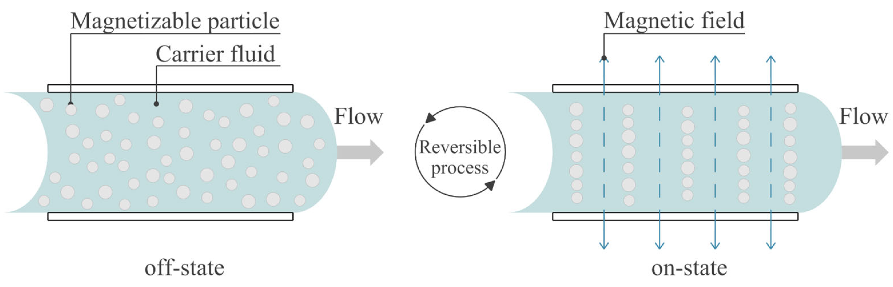
When a magnetic field is applied, three effects occur. First, the magnetic nanoparticles align along the magnetic field lines [
27]. This alignment can increase the internal resistance to flow, effectively increasing the viscosity of the fluid. Second, at higher field strengths, the particles may form chains or structures along the field lines. These structures disrupt the fluid flow, leading to a significant increase in viscosity. In some cases, the fluid can exhibit non-Newtonian behavior, with the viscosity depending on the shear rate [
28,
29]. Third, the dependence of viscosity on the strength of the applied magnetic field is known as the magnetoviscous effect. This relationship is typically nonlinear: small increases in field strength can cause significant changes in viscosity [
30]. These effects occur when the magnetic field is activated, also known as the on-state. The chain-like arrangement is a reversible process, and particles flow freely when the magnetic field is no longer activated (off-state). This behavior is depicted in
Figure 5.
Several factors affect how viscosity changes under a magnetic field. Higher particle concentrations lead to more pronounced viscosity changes, while larger particles or broader size distributions can enhance alignment and chain formation. Stronger magnetic fields cause more alignment and structure formation. Higher temperatures can reduce the effect of the magnetic field due to increased thermal agitation. The properties of the carrier fluid also influence the overall magnetoviscous behavior. It must be noted that the temperature alone is a parameter that can significantly alter the fluid viscosity, depending on its specific properties. For this reason, in this work the temperature has been controlled throughout the tests and has been included in the analysis to account for its potential influence on viscosity variation.
Several authors have investigated the dependence of magnetic fluid viscosity on external magnetic fields, employing both theoretical and experimental approaches. Shen and Doi [
31] calculated the effective viscosity of magnetic fluids at the particle scale. They compared their results with classical constitutive equations and proposed a new equation according to their numerical findings. Patel [
32] investigated the simultaneous effects of magnetic field and temperature on the capillary viscosity of magnetic nanofluids. The study provided experimental data and proposed theoretical explanations for the observed changes in effective viscosity under varying magnetic field strengths and orientations. Additionally, Patel et al. [
33] measured the effective viscosity of a ferrofluid as a function of an applied magnetic field oriented perpendicular to the capillary flow. Their findings showed close agreement with the Shliomis [
34] expression, derived using the effective field method, providing insights into how the viscosity changes with varying magnetic field strengths. Polunin et al. [
35] estimated the viscosity increment in a magnetic fluid column oscillating under a strong transverse magnetic field. The authors calculated viscosity using expressions derived from different theoretical approaches and analyzed the impact of the magnetic field on the fluid’s viscosity.


 ,
, 


