Significance in Numerical Simulation and Optimization Method Based on Multi-Indicator Sensitivity Analysis for Low Impact Development Practice Strategy

Abstract

Evaluating the performance of sponge city practices under actual conditions is essential for managing urban stormwater. Existing studies in urban stormwater management have rarely employed numerical simulations to model hydrological processes under actual Three-Dimensional (3D) conditions. In this study, a numerical computational model is developed to simulate the hydrological processes and reveal the temporal and spatial variation of runoff in relation to impervious surfaces and concave herbaceous fields. The applicability of the 3D modules was evaluated using the Chicago rain pattern formula under three recurrence periods: precipitation within one, five, and ten years. The results indicate that the thickness and slope of planting soil are the most sensitive factors regarding sponge city performance, with comprehensive factors of 0.754 and 0.461. The optimal structural parameters of the concave herbaceous field were obtained as follows: aquifer height, 200 mm; planting soil thickness, 600 mm; planting soil slope, 1.5%; planting soil porosity, 0.45; overflow pipeline porosity, 0.3. The flood peak reduction rate, delay rate, and total runoff control rate were the best in a recurrence period of 5a, with 88.93%, 51.11%, and 78.76%, respectively. This study offers technical and conformed methodological support for simulating water quantity processes in sponge cities, and for the control of waterlogging and the recycling of runoff.

1. Introduction

Traditional urban development focuses on high-intensive, hardened land utilization and can damage the natural water cycle, which significantly increases surface runoff and increases the urban waterlogging risk [1]. Sponge cities aim to protect the original ecological structures, including lakes, rivers, greenbelt, etc., to maintain the natural hydrological characteristics before urbanization [2]. Low Impact Development (LID) practices are designed to reduce stormwater runoff at the source level in terms of decreasing flow volume rate and delaying peak value [3]. Although many studies have reported the availability of experimental or numerical models for simulating the rain-flood control capability of LIDs under actual precipitation conditions, only a few piece of research have been conducted on a Three-Dimensional (3D) scale to demonstrate the specific migration process of runoff in LIDs [4,5,6]. LID modeling tools tend to need improvement in order to better adapt to the increasing complexity between impervious buildings and green infrastructure, so that the growing LID implementation can be optimally designed and performed [7,8].

Numerical models are critical tools for simulating hydrological processes in LID practices, yet their application in Three-Dimensional (3D) scenarios remains limited. While models such as SWMM, SWAT, and SUSTAIN have advanced stormwater management by evaluating regional-scale runoff control (e.g., permeable pavements and bioretention systems) [9,10,11,12,13], they predominantly focus on aggregated performance rather than the detailed 3D hydraulic behaviors of individual LID facilities. For instance, Hakimdavar et al. [14] and Feitosa and Wilkinson [15] selected green roofs with three spatial scales and utilized HYDRUS-1D to examine the applicability of a one-dimensional infiltration model in predicting hydrologic behavior, and they found that the performance of runoff control improves as the green roof drainage area increases. Baek et al. [16] developed a piece of simulation modeling software to optimize bioretention in the watershed. Using the Flow Duration Curve (FDC), their results indicated that the location and size of bioretention and the soil texture together have the most significant impact on the benefits of LIDs, yet their 1D or 2D approaches failed to capture complex 3D flow dynamics.

To address this gap, Computational Fluid Dynamics (CFDs) provides a robust framework for resolving 3D flow fields through Navier–Stokes equations and turbulence models, enabling precise visualization of infiltration, drainage, and overflow processes. However, CFD models are sensitive to empirical parameters (e.g., soil porosity, slope), necessitating systematic sensitivity analysis. Here, the local Morris parameter sensitivity analysis method is introduced to quantify the influence weight of structural parameters (such as matrix layer thickness and slope) on the overflow and peak flow [17]; furthermore, the TOPSIS multi-objective decision model is used to prioritize the parameter combination schemes according to the positive and negative ideal solution distance [18,19]. This method not only makes up for the deficiency of the traditional model in the analysis accuracy of single facilities but also overcomes the empirical dependence of parameter optimization through sensitivity–benefit collaborative analysis.

The present study first utilized numerical simulation at the 3D level and, combined with local Morris parameter sensitivity, TOPSIS methods to adjust the structural indicators of concave herbaceous fields, which are typical LIDs. In this research, the precipitation process and volume were calculated by the rainfall characteristics of Tianjin and the Chicago precipitation pattern formula. Then, the reduction of overflow volume and peak flow were analyzed through LID schemes with different parameters, utilizing the continuity equation, the momentum equation, and Darcy’s law, calculated in a numerical model. The sensitivity discriminant factors and the priority values of each plan were subsequently obtained by analyzing the flow decrease and applying the local Morris parameter sensitivity analysis and TOPSIS. After obtaining the most significant parameter and the optimal scheme, three storm events were used to simulate the runoff control effect of the concave herbaceous field under the best plan. Meanwhile, its stormwater control process, benefits, and application methods under actual working conditions were acquired. The proposed model and analysis framework could help to simulate the practical performance of sponge cities under actual precipitation conditions and provide technical references for buildings and the optimization of LID facility structures in the subsequent sponge city construction.

2. Materials and Methods

2.1. Research Data Background

The research data, including precipitation characteristics, facility parameter standards, and soil structure, were prepared based on a coastal urban area in Tianjin, China. Tianjin is located on the east coast of the middle latitude warm temperate continent of Eurasia, and the climate type is the monsoon climate of a semi-humid temperate zone. According to the data of the past ten years, from 2013 to 2022, the annual precipitation is about 450–950 mm, the average annual precipitation is about 670 mm, and the average annual evaporation is about 770 mm; the overall climate is relatively dry. The precipitation in Tianjin is mainly concentrated in June, July, and August of the summer, which can account for about 75% of the annual precipitation. The soil is mainly silty clay, with good water retention and poor permeability, and the permeability coefficient is between 8.8 × 10⁻⁶ and 1.3 × 10⁻³ cm/s. The land use type in the downtown area is mainly hardened surface, of which impervious surfaces such as buildings and concrete pavement accounts for 80.23%. The amount of ecological underlying surfaces, such as green space and water area, is relatively low, accounting for only 10.53% (Figure 1).

2.2. Design of Simulated Precipitation Events

The calculation and analysis process of the numerical model is mainly supported by precipitation data to explore the hydraulic migration process of precipitation runoff in LID facilities and further calculate the total overflow flow, peak flow, and peak time of the drainage outlet. Generally speaking, it is difficult to obtain precipitation data with a long duration in a particular region, and it is also difficult to obtain large and extremely heavy rain data through measurement. Therefore, in the study of various stormwater management numerical models, the Chicago rain pattern Formulas (1) and (2), based on the local rainstorm intensity characteristics, is often used to generate the precipitation process data in the study area, so they can be applied to the actual numerical analysis and calculation. This method has been applied in many sponge city studies in the past; it has sufficient science and rationality and fits the practice. Sponge city facilities are generally mainly used to deal with the runoff problems generated by small, medium, and large precipitation or short-term heavy precipitation, but they are not suitable for precipitation under rare extreme events [20]. Combined with the applicable field and scope of LID facilities, precipitation processes with small, medium, and large precipitation characteristics lasting 2 h and recurrence periods of 1a, 5a, and 10a were selected in this paper as the basic data for the three-dimensional hydraulic numerical analysis of runoff of the concave herbaceous field. In addition, the precipitation intensity at the early and late stages of the rainfall-type process in Chicago is relatively small, the concave herbaceous field can absorb all the runoff, and there is no obvious water flow through the overflow well and drainage outlet, so the simulation results are not significant. Therefore, in this paper, the most significant precipitation process of 60 min before and after the rain peak in the whole precipitation process, with a total of 120 min, was selected for numerical analysis and calculation. This allowed analysis of the most significant runoff reduction and flood peak control effect of the drainage outlet.

2.3. Model Construction and Structural Parameter Setting

2.3.1. Computational Grid Construction

Using complete N–S (Navier–Stokes) equations, Tru-VOF, FDM with FAVOR, and other methods, numerical simulation can accurately predict the free liquid surface flow and visualize the results. The basic idea is as follows: The drainage basin is divided into multiple grids that define flow parameters at discrete locations, such as pressure, temperature, and velocity, and these can be used to perform numerical simulations of the values of the equations of fluid motion. The distribution of basic physical quantities and the change of physical quantities with time can be obtained by numerical simulation. The finite difference/control volume method is used to generate structured mesh, and the multi-grid block and superimposed block technology are used to make the mesh more compact. The precision can be set with different blocks, and the complex structural features can be described with the appropriate number of grids.

2.3.2. Physics Modeling and Boundary Conditions

In this study, the concave herbaceous field is selected as a LID facility. The concave herbaceous field is used to collect the runoff generated by the surrounding hardened surface and achieve the purposes of runoff, flood peak reduction, and flood peak delay through the rainwater retention and infiltration of the soil and gravel layers in its structural layer. The working principle is as follows: During the rainfall process, the ground rainwater is collected into the green belt of the planting soil and is permeated and stored through the planting soil. The excess rainwater flows into the underground space through the vertical well and is discharged through the transverse seepage pipe. The results show that the rainwater control efficiency of the concave green space is significantly related to the depth of the concave, the thickness of the planting soil, the thickness of the gravel layer, the slope of the planting soil, the porosity of the planting soil, the porosity of the drainage pipe, and the recurrence period of the designed rainstorm (Figure 2a).

The medium-sized concave herbaceous field is taken as the model calculation area under actual working conditions. The model is 300 m long and 60 m wide (Figure 2b). The physical modules involved in the calculation include gravity module, porous media module, viscous flow module, and turbulent flow module. The boundary condition of the model inlet adopts the velocity boundary, and the design water level of the initial condition is equal to the ground height of the inlet. The front and back sides of the seepage structure layer and the top of the model are set as impervious solid wall boundaries. The side wall itself is impervious to water, and the outer side is set as a continuous boundary, which can only allow water flow out of the drainage seepage pipe. The bottom of the model is set as a continuous boundary, which allows the structural layer to seep rainwater out. The total duration of the simulated precipitation scenario is 2 h, and the initial time step is set to 1 min. The minimum time step is the default value. In addition, the flow monitoring surface is set at the mouth of the green drainage pipe; this allows one to judge the stormwater control effect of LID facilities more intuitively through the total runoff overflow characteristics of the overall structure.

Moreover, in order to explore the runoff control benefits and optimization schemes of the concave herbaceous field with different structure layer sizes, the initial dimensions of each structure layer were set according to relevant norms and literature, as shown in

Table 1. The initial dimensions of each structural layer of the concave green space.

ID	A	B	C	D	E
Structure parameter name (unit)	Aquifer height (mm)	Planting soil thickness (mm)	Slope of planting soil (%)	Planting soil porosity (%)	Pipeline porosity (%)
Initial size	200	600	1.5	45	30
Value range	100~300	250~1000	1~3	30~60	>20

.

2.4. Parameter Perturbation and Sensitivity Analysis

In this study, the optimization method adopted is to use the parameter perturbation method in the parameter sensitivity analysis method to set up a series of concave green spaces with different structural sizes and combine the TOPSIS optimization method to screen the most significant benefits.

Six structural parameters of the concave herbaceous field were selected for sensitivity analysis: depth of the concave area, thickness of the planting soil layer, thickness of the gravel layer, slope of the planting soil, porosity of the planting soil, and porosity of the drainage pipe. Among them, the sensitivity of model parameters can be divided into local sensitivity and global sensitivity [21]. The local sensitivity represents the impact of a single parameter change on the model results, while the global sensitivity represents the comprehensive impact of multiple parameter changes on the model results and includes interactions between several parameters. Global sensitivity analysis can comprehensively analyze the influence of each parameter, but it is difficult to apply to most complex models with more parameters because of the difficulty of calculation. Therefore, to isolate the effect of individual parameters, the modified Morris local sensitivity analysis was employed. Each parameter was perturbed by ±30% from its initial value (Table 1) in 10% increments, while holding other parameters constant. Simulations were conducted under a 1-year return period rainfall scenario (Section 3.2), with outcomes evaluated through three metrics: total runoff reduction rate, peak runoff reduction rate, and peak time delay rate.

2.5. Formulas and Calculations

2.5.1. Design Storm Scenarios

According to the “Technical Guidelines for the Construction of Sponge City in Tianjin” [22], the study area is located within the first division of Tianjin rainstorm intensity, and the design is as follows:

$$q={\displaystyle \frac{2141(1+0.7562\lg P)}{{(t+9.6093)}^{0.6893}}}$$

(1)

where $q$ is design storm intensity (L/s · ha), $P$ is recurrence period (1 ≤ P ≤ 100, a), and $t$ is precipitation duration (5 ≤ t ≤ 180, min).

Meanwhile, the conversion formula of rainstorm intensity $i$ and $q$ is:

$$i={\displaystyle \frac{q}{167}}$$

(2)

where $i$ is storm intensity (mm/min).

2.5.2. Governing Equation of Fluid Motion

The governing equation of incompressible fluid motion in numerical simulation adopts the N–S equation, and the governing equation of water flow (including continuity equation and momentum equation) is established based on the Cartesian coordinate system:

The Cartesian coordinates are generally as follows: Xmin—left boundary, Xmax—right boundary, Ymin—front boundary, Ymax—back boundary, Zmin—bottom boundary, Zmax—top boundary.

The Continuity equation:

$${\displaystyle \frac{\partial (u{A}_x)}{\partial x}}+{\displaystyle \frac{\partial (v{A}_y)}{\partial y}}+{\displaystyle \frac{\partial (w{A}_z)}{\partial z}}=0$$

(3)

Momentum equations:

$${\displaystyle \frac{\partial u}{\partial t}}+{\displaystyle \frac{1}{V_F}}\left\{u{A}_x{\displaystyle \frac{\partial u}{\partial x}}+v{A}_y{\displaystyle \frac{\partial u}{\partial y}}+w{A}_z{\displaystyle \frac{\partial u}{\partial z}}\right\}=-{\displaystyle \frac{1}{\rho }}{\displaystyle \frac{\partial p}{\partial x}}+G_x+f_x$$

(4)

$${\displaystyle \frac{\partial v}{\partial t}}+{\displaystyle \frac{1}{V_F}}\left\{u{A}_x{\displaystyle \frac{\partial v}{\partial x}}+v{A}_y{\displaystyle \frac{\partial v}{\partial y}}+w{A}_z{\displaystyle \frac{\partial v}{\partial z}}\right\}=-{\displaystyle \frac{1}{\rho }}{\displaystyle \frac{\partial p}{\partial y}}+G_y+f_y$$

(5)

$${\displaystyle \frac{\partial w}{\partial t}}+{\displaystyle \frac{1}{V_F}}\left\{u{A}_x{\displaystyle \frac{\partial w}{\partial x}}+v{A}_y{\displaystyle \frac{\partial w}{\partial y}}+w{A}_z{\displaystyle \frac{\partial w}{\partial z}}\right\}=-{\displaystyle \frac{1}{\rho }}{\displaystyle \frac{\partial p}{\partial z}}+G_z+f_z$$

(6)

where $u$, $v$, and $w$ are the velocity component in the x, y, and z directions, respectively; $A_x$, $A_y$, and $A_z$ are the area of the section through which the fluid flows; $G_x$, $G_y$, $G_z$ are the acceleration in the x, y, and z directions; $f_x$, $f_y$, $f_z$ are the acceleration of the viscous force in the x, y, and z directions; $V_F$ is the volume fraction of the fluid through which the unit is calculated; $\rho$ is the fluid density; and $p$ is the pressure acting on the fluid element.

2.5.3. Viscous Turbulence Model

The commonly used temperature flow models for hydraulic numerical simulation include Prandtl mixing length, one-equation, two-equation k−ε, RNG (Renormalization-Group), k−ω, and LES models. In this study, the RNG model, a commonly used model in hydraulic engineering and hydraulics research, is adopted. Its formula has more accurate theoretical values and can simulate low-intensity turbulence and complex vortex flow, so it is relatively widely used. Its governing equation are as follows [23]:

Turbulent kinetic energy k equation:

$${\displaystyle \frac{\partial (\rho k)}{\partial t}}+{\displaystyle \frac{\partial (\rho k{u}_i)}{\partial x_i}}={\displaystyle \frac{\partial }{\partial x_j}}\left[\left(\mu +{\displaystyle \frac{{\mu }_t}{{\sigma }_k}}\right){\displaystyle \frac{{\partial }_k}{\partial x_j}}\right]+G_k+\rho \epsilon$$

(7)

Turbulence kinetic energy dissipation rate equation:

$${\displaystyle \frac{\partial (\rho \epsilon )}{\partial t}}+{\displaystyle \frac{\partial (\rho \epsilon u_i)}{\partial x_i}}={\displaystyle \frac{\partial }{\partial x_j}}\left[\left(\mu +{\displaystyle \frac{{\mu }_t}{{\sigma }_{\epsilon }}}\right){\displaystyle \frac{\partial \epsilon }{\partial x_j}}\right]+{\displaystyle \frac{C_{1\epsilon }^{*}}{k}}{G}_k-C_{2\epsilon }{\displaystyle \frac{{\epsilon }^2}{k}}$$

(8)

$$\left\{\begin{array}{l}{G}_k={\mu }_t\left({\displaystyle \frac{\partial u_i}{\partial x_j}}+{\displaystyle \frac{\partial u_j}{\partial x_i}}\right){\displaystyle \frac{\partial u_i}{\partial x_j}}\\ C_{1\epsilon }^{*}=C_{1\epsilon }-{\displaystyle \frac{\eta (1-\eta /{\eta }_0)}{1+\beta {\eta }^3}}\\ \eta ={(2E_{ij}\cdot E_{ij})}^{1/2}{\displaystyle \frac{k}{\epsilon }}\\ E_{ij}={\displaystyle \frac{1}{2}}\left({\displaystyle \frac{\partial u_i}{\partial x_j}}+{\displaystyle \frac{\partial u_j}{\partial x_i}}\right)\end{array}\right.$$

(9)

where ${\mu }_t$ is the kinematic viscosity coefficient of turbulence, ${\mu }_t=C_{\mu }{k}^2/\epsilon$, $C_{\mu }$ = 0.085, ${\sigma }_k$ = ${\sigma }_{\epsilon }$ = 0.7179, and $G_k$ is the turbulent kinetic energy generation term: $C_{1\epsilon }$ = 1.42, $C_{2\epsilon }$ = 1.68, ${\eta }_0$ = 4.377, $\beta$ = 0.012.

2.5.4. Morris Sensitivity Analysis

In Fan et al. [24], the Morris screening method was used, meaning that a parameter $x_i$ is selected from the research parameters. The parameter is then randomly distributed within the selected range, the model is run separately under each disturbance parameter condition, and the corresponding output result $y(x)=y(x_1,x_2,x_3,\cdots ,x_n)$ is obtained. The influence value $e_i$ is further used to represent the influence of each parameter on the simulation result:

$$e_i=(y_i-y)/\Delta i$$

(10)

where $y_i$ is the output value after the parameter change, $y$ is the output value before the parameter change, and $\Delta i$ is the change amplitude of parameter $i$.

Moreover, the modified Morris rule is used to obtain multiple sensitivity coefficients of the parameters by perturbing the independent variable parameters with fixed step percentage. The average value of the sensitivity coefficients is then used as the result discrimination factor:

$$SN={\displaystyle \frac{{\displaystyle {\sum }_{i=0}^{n-1}\frac{(Y_{i+1}-Y_i)/Y_0}{(P_{i+1}-P_i)/100}}}{n}}$$

(11)

where $SN$ is sensitivity discriminant factor, $Y_{i+1}$ is the output value of the target variable for the i + 1 run of the model, $Y_i$ is the output value of the target variable for the i run of the model, $Y_0$ is the output value of the target variable when the parameter takes the reference value, $P_{i+1}$ is the percentage change of the parameters of the i + 1 run of the model compared to the initial value, $P_i$ is the percentage change of the parameters of the i run of the model compared to the initial value, and $n$ is the model run times.

According to the value of parameter $\left|SN\right|$, sensitivity can be divided into four categories: $\left|SN\right|$ ≥ 1, very sensitive parameter; 0.2 ≤ $\left|SN\right|$ < 1, high sensitive parameters; 0.05 ≤ $\left|SN\right|$ < 0.2, medium sensitive parameter; 0 ≤ $\left|SN\right|$ < 0.05, insensitive parameter.

2.5.5. TOPSIS Optimal Solution Analysis Method

The TOPSIS method is a famous classic multi-criteria decision analysis method that can make full use of research target attributes and information to rank different schemes, and it does not require preference independence. According to the maximum distance from the positive ideal solution to the negative ideal solution, the alternative solutions are prioritized. If the evaluation object is closest to the optimal solution and farthest from the worst solution, it is the best; otherwise, it is not the best [25]. The main calculation steps are as follows:

Weighted normalized decision matrix construction:

The weighted normalized decision matrix $Z={(Z_{ij})}_{m\times n}$ can be obtained by multiplying the index standardization matrix $A^{\prime }$ with weight $w_i$:

$$Z_{ij}=A_{ij}\prime w_i(i=1,2,\cdots ,\mathrm{m};\mathrm{j}=1,2,\cdots ,\mathrm{n})$$

(12)

Determine the positive ideal solution $X_i^{+}$ and the negative ideal solution $X_i^{-}$:

$$X_i^{+}=(X_1^{+},X_2^{+},\cdots ,X_m^{+})$$

(13)

$$X_i^{-}=(X_1^{-},X_2^{-},\cdots ,X_m^{-})$$

(14)

The formula for calculating the positive and negative ideal solutions of the positive indicators is as follows: $\left\{\begin{array}{l}{X}_i^{+}=\max Z_{ij}\\ X_i^{-}=\min Z_{ij}\end{array}\right.$. The formula for calculating the ideal solution of the negative indicators is $\left\{\begin{array}{l}{X}_i^{+}=\min Z_{ij}\\ X_i^{-}=\max Z_{ij}\end{array}\right.$.

The Euclidean distances, $S_j^{+}$ and $S_j^{-}$, of each evaluation object to positive and negative ideal solutions are calculated separately.

The Euclidean distance formula is used to calculate the distance from the standardized vector of each evaluation index to the optimal solution and the worst solution, respectively:

$$S_j^{+}=\sqrt{{\displaystyle {\sum }_{i=1}^m{(Z_{ij}-X_i^{+})}^2}}$$

(15)

$$S_j^{-}=\sqrt{{\displaystyle {\sum }_{i=1}^m{(Z_{ij}-X_i^{-})}^2}}$$

(16)

Calculate the relative proximity between each evaluation object and the optimal scheme:

$$D_j={\displaystyle \frac{S_j^{-}}{S_j^{+}+S_j^{-}}}$$

(17)

where $D_j$ is the comprehensive evaluation score of each evaluation object. The larger value indicates that the evaluated object is closer to the ideal solution and the benefit level is better; a smaller value indicates that the evaluated object is farther from the ideal solution and the benefit level is worse.

3. Results and Discussion

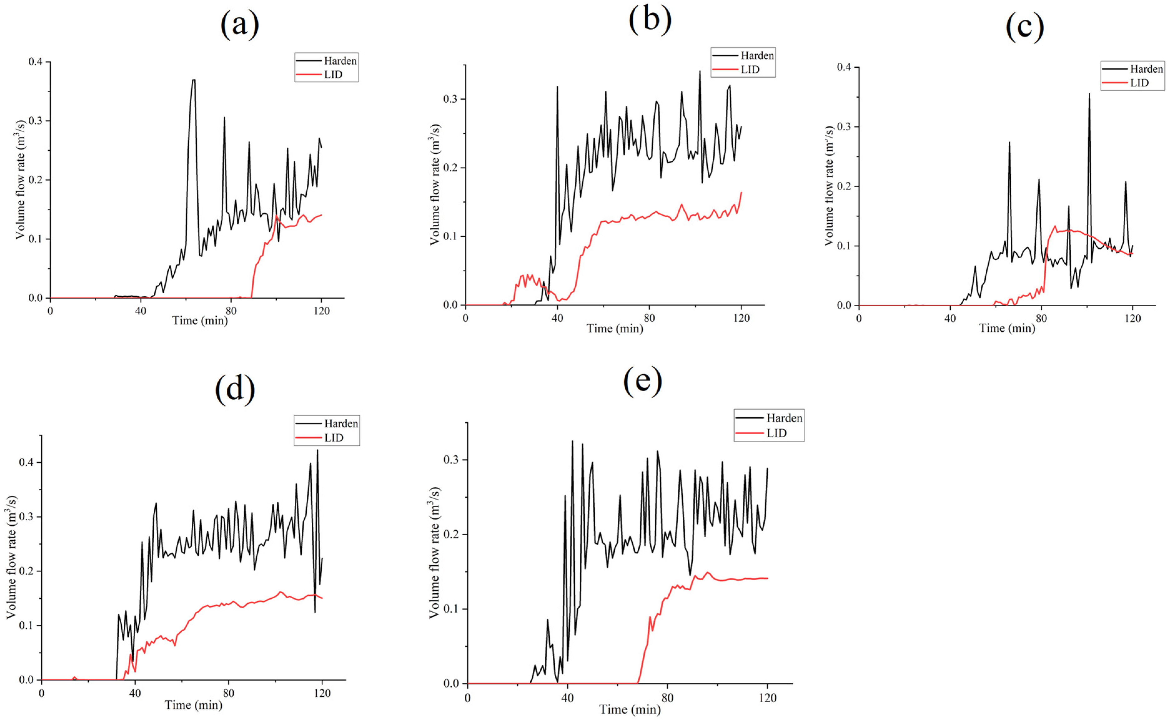
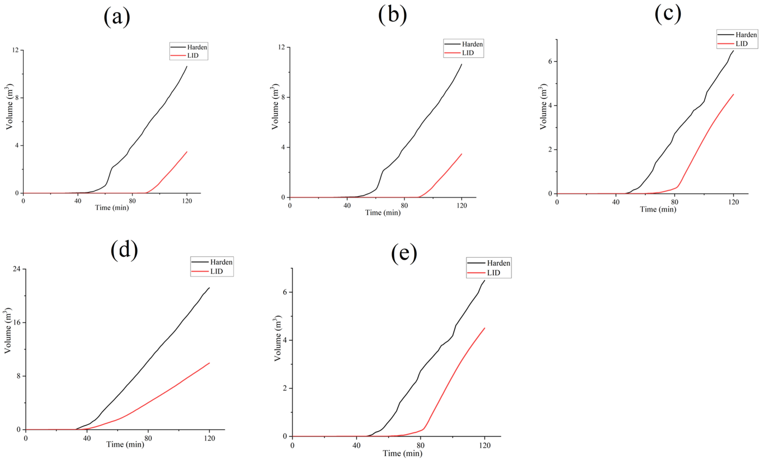
3.1. Simulation of Runoff Infiltration and Storage Process

During the process of rainwater collection, retention, and discharge in the concave herbaceous field, the runoff generated by rainwater first gathers from the road surface on one side of the green space and flows into the green space aquifer after a short drop in the curb height under the action of gravity. The runoff then permeates vertically through the planting layer and collects at the end of the green space along the slope contained in the planting soil (slope from high to low inclined overflow wells). The excess rainwater beyond the permeability of the layer is collected through the overflow wells at the end. The lateral seepage pipe is arranged at the bottom side of the overflow well, which can discharge the rainwater collected from the overflow well through the drainage pipe. At the same time, the seepage effect on the side of the pipe and the rainwater from the planting soil will further percolate into the base soil to enhance the runoff absorption effect. In addition, the end of the seepage drainage pipe can be connected to a water storage structure, such as a reservoir, in order to make full use of the collected rainwater resources, to achieve the purpose of combining the drainage and storage functions of the sponge city. Moreover, in order to compare the changes of runoff characteristics (including peak runoff and peak generation time) generated by rainwater before and after the implementation of the concave herbaceous field, a “hardened structure” of the same size is set for each concave herbaceous field scheme as the “hardened surface” control group of LID facilities. The difference in stormwater runoff transport between traditional urban development mode and low impact development mode is more directly compared.

3.2. Parameter Sensitivity Calculation and Effect Analysis

In order to reflect the sensitivity of structural parameters under different types of benefits of runoff control, the precipitation scenario with a return period of 1 year, as set in Section 2.4, was selected to simulate the runoff characteristics. The initial values of each structural parameter and disturbance values were compared, as shown in

Table 2. Initial value and disturbance value of structural parameters.

Disturbance Ratio (%)	−30	−20	−10	0 (Initial)	10	20	30
Indicator
A	140	160	180	200	220	240	260
B	450	480	540	600	660	720	780
C	1.05	1.20	1.35	1.50	1.65	1.80	1.95
D	31.50	36	40.50	45	49.50	54	58.50
E	21	24	27	30	33	36	39

. In the 1a precipitation scenario, the sensitivity analysis results of each parameter based on the three benefits of total runoff reduction rate, peak runoff reduction rate, and peak time delay rate of the overflow pipe outlet are shown in Figure 3.

Based on the analysis of Formula (11), it can be seen that the sensitivity types of parameters of the concave herbaceous field can be divided into highly sensitive parameters, sensitive parameters, medium sensitive parameters, and insensitive parameters. In this study, the $\left|SN\right|$ of the sensitivity analysis results of each parameter is basically >0.05, that is, all of them have a certain sensitivity and are not insensitive parameters without analytical significance. Different kinds of benefits of runoff control have different effects on the sensitivity of the structural parameters of the concave herbaceous field. For example, when the flood peak function is reduced, the sensitivity of the pipeline porosity is much higher than the flood peak time delay and total runoff reduction (Figure 3a), while the sensitivity of the planted soil slope is completely opposite. Under the scenario aimed at flood peak delay and total overflow reduction, the parameters of planted soil porosity and slope are highly sensitive, while planted soil thickness is highly sensitive under the flood peak delay function (Figure 3b); meanwhile, aquifer height is highly sensitive under the total overflow reduction benefit (Figure 3c).

It is not difficult to understand that the increase in the peak discharge value of the drainage outlet often means that the area of the runoff and the drainage seepage pipe increases, or the water pressure value in the pipeline increases. Obviously, the reduction degree at the outlet of the pipeline mainly depends on the seepage amount of water in the pipeline, that is, the size of the porosity. Therefore, the benefit of flood peak reduction is closely related to the nearest drainage seepage pipe. However, the structure that is far away from the drainage outlet of planting soil and the aquifer has less of a relationship, so the parameter sensitivity is lower. In terms of flood peak delay and total overflow reduction, the rainwater retention function of the concave herbaceous field mainly depends on the water storage capacity of the planting soil, while the storage space of seepage water depends mainly on the space between soil particles. When the porosity is sufficient, the infiltrated runoff and rainwater can be trapped more effectively in the planting soil. As a result, the runoff water generated in the early precipitation period is mainly held and stored by the soil, delaying the time of flood peak generation and reducing the total overflow flow. At the same time, the slope affects the migration time of runoff on the planted soil surface, and a smaller slope can give runoff and rainwater more time to contact the soil surface and improve the infiltration efficiency of water. It is also revealed that the flood peak time and the total overflow flow mainly depend on the runoff characteristics when entering the overflow wellhead and are closer to the structure of the planting soil. Therefore, the sensitivity of the two runoff control benefits to the structural parameters of the larger planting soil is higher, while the sensitivity to the porosity of the smaller pipeline structure is lower. In addition, the thickness of the planting soil is closely related to the efficiency of the temporary retention of rainwater. Thicker soil means that the time of absorbing pre-runoff water is more “lasting” and the time of the delayed peak is longer. Therefore, its sensitivity to flood peak delay is more obvious. On the other hand, the main function of the aquifer exposed to the air above the planted soil is to collect and temporarily store rainwater from the road surface. Under a certain simulated precipitation time, the higher the height of the aquifer, the more water it can retain, and the less water will enter the overflow well and accumulate in the drainage outlet at a certain time. Therefore, its sensitivity to the total flow reduction rate is also high.

However, according to the sensitivity analysis of the above parameters, the sensitivity of the concave herbaceous field model to the parameters of total runoff reduction rate, peak runoff reduction rate, and peak time delay rate is quite different. In order to more objectively evaluate the comprehensive sensitivity of the parameters of the concave herbaceous field structure to each benefit simulation project, the coefficient of variation method (information weight method) was used to determine the weights of different simulation results, and then the weights were used to calculate the comprehensive sensitivity coefficients of each parameter. The calculated results are shown in

Table 3. Information weight method calculation results.

Indicator	Mean Value	Standard Deviation	Coefficient of Variation	Weight	Composite Coefficient
A	0.644	0.194	30.18%	6.47%	0.2274
B	1.078	1.320	122.37%	26.25%	0.7536
C	0.700	0.839	119.94%	25.73%	0.4613
D	0.727	0.623	85.66%	18.37%	0.2008
E	0.366	0.396	108.06%	23.18%	0.0848

, and the comprehensive sensitivity coefficients are shown in Figure 3d. The results of comprehensive parameter sensitivity analysis showed that the thickness of the planted soil, slope, and aquifer height were highly sensitive factors regarding the runoff control efficiency of the concave herbaceous field, while the comprehensive sensitivity of planted soil porosity and seepage pipe porosity was low. Combined with the above analysis and the analysis of geographical factors such as soil permeability in Tianjin, the basic soil permeability in the study area is poor, and LID facilities focusing on permeability do not sufficiently fulfil their function of runoff control. In this study, the runoff regulation ability of the concave herbaceous field mainly focuses on the temporary water storage function of aquifers, the infiltration process of the planting soil itself, the retention of rainwater and the overflow drainage process of drainage pipes, and the runoff seepage through the lower gravel layer of the planting soil. In addition, the original soil is less. Therefore, the porosity of the planting soil and the drainage seepage pipe, which are closely related to the infiltration process, can play a limited role, and the contribution and parameter sensitivity to the overall runoff control benefit of the concave herbaceous field are small. Therefore, the parameter optimization and transformation of the concave green space should mainly focus on the planting soil thickness, slope, and aquifer height with the most significant comprehensive parameter sensitivity. According to the sensitivity analysis results of comprehensive parameters, the runoff control benefits of each scheme with different parameters are further ranked by the optimization method, so as to explore the optimal structural parameters of the concave herbaceous field.

3.3. LID Performance Evaluation and Sorting Optimization Based on TOPSIS

In the results of the parameter sensitivity analysis, the structural parameters that have the most significant impact on the concave herbaceous field have been obtained. In order to determine the optimal choice of benefits among the different schemes formulated according to parameter changes, the TOPSIS optimal solution ranking method and Formulas (12)–(17) were used to further sort and comprehensively optimize the benefit results generated by the numerical simulation of each scheme. The TOPSIS analysis results of three kinds of runoff control benefits based on the disturbance change of flood peak reduction rate, flood peak time delay rate, and total overflow reduction rate are shown in

Table 4. Flood peak reduction rate corresponds to the TOPSIS analysis results of parameter disturbance change.

Disturbance Ratio	Positive Ideal Solution Distance D+	Negative Ideal Solution Distance D−	Relative Proximity C	Sort Result
−30%	0.311	0.281	0.475	2
−20%	0.406	0.308	0.432	4
−10%	0.387	0.300	0.436	3
0%	0.450	0.223	0.331	6
10%	0.366	0.211	0.366	5
20%	0.452	0.192	0.298	7
30%	0.233	0.487	0.677	1

,

Table 5. The time delay rate of the flood peak corresponds to the TOPSIS analysis results of parameter disturbance change.

Disturbance Ratio	Positive Ideal Solution Distance D+	Negative Ideal Solution Distance D−	Relative Proximity C	Sort Result
−30%	0.113	0.029	0.205	5
−20%	0.134	0.009	0.062	7
−10%	0.072	0.113	0.610	1
0%	0.130	0.010	0.069	6
10%	0.105	0.035	0.250	4
20%	0.100	0.049	0.328	3
30%	0.098	0.080	0.448	2

and

Table 6. Total overflow reduction rate corresponds to the TOPSIS analysis results of parameter disturbance change.

Disturbance Ratio	Positive Ideal Solution Distance D+	Negative Ideal Solution Distance D−	Relative Proximity C	Sort Result
−30%	0.200	0.397	0.665	1
−20%	0.381	0.234	0.381	7
−10%	0.235	0.320	0.577	4
0%	0.321	0.335	0.511	5
10%	0.243	0.352	0.592	3
20%	0.214	0.349	0.619	2
30%	0.362	0.329	0.476	6

.

The results show that, for flood peak reduction rate, when the parameter disturbance rate is 30%, −30%, and −10%, the concave green space benefit ranking is better. In terms of the time delay rate of the flood peak, the efficiency order is the best when the disturbance rate is −10%, 30%, and 20%. From the perspective of the total flow reduction rate, the efficiency of the green space under the disturbance rate of −30%, 20%, and 10% is more advanced. For the first case, the reason for this may be that, when there is a large planting soil thickness and aquifer height or a small planting soil slope, the rainwater runoff collected by the road surface is more likely to be absorbed and retained by the planting soil layer, resulting in a significant reduction of the maximum runoff generated at the drainage outlet, thereby improving the efficiency of flood peak reduction. In the second case, when the thickness parameters of the aquifer and the planting soil are more balanced or both are higher, the runoff generated in the early precipitation process will be able to remain in the aquifer and planting soil for a longer time, thus significantly delaying the generation time of runoff and flood peak caused by rain peak. In addition, in the third case, the reduction effect of total discharge may be more closely related to the slope of the planted soil. Although the thickness of the soil and the height of the aquifer decrease, the gentle topography makes the collected runoff converge more slowly to the overflow well at the end of the green space, and the total discharge at the drainage outlet also significantly decreases under the same simulated time node.

The TOPSIS optimization results of the above three kinds of benefits have obvious differences, but there are also similarities. When the parameter disturbance value is at a small level, the benefit optimization analysis results of LID facilities under different kinds of benefits are good. Through comprehensive and comparative analysis, a more balanced parameter disturbance range of −10~10% is selected as the optimal result of the optimization sorting analysis. The runoff control efficiency of different schemes under the parameter variation range was further compared and analyzed.

3.4. LID Scenario Analysis and Benefit Evaluation

3.4.1. Simulation Effects of the LID Plans Under Different Structural Parameters

According to the above analysis results, due to the highly comprehensive parameter sensitivity of the aquifer, the thickness and slope of the planting soil are significantly smaller, and the aquifer itself does not belong to the solid structural layer and the influence effect is similar to that of planting soil thickness, so the comparison and optimization design of runoff control benefits for the concave green space mainly focus on the latter two. Figure 4 shows the runoff characteristics of the green space and the hardened surface under the initial parameters (parameter disturbance rate 0) and the control hardened surface with disturbance rate of −10% and 10% compared to the planted soil thickness and the planted soil slope of −10% and 10% structural parameters under the precipitation scenario of the 1a recurrence period. As can be seen from Figure 4b,d, after the implementation of LID facilities, the real-time runoff of the overflow drainage outlet is significantly reduced, and the peak value is less obvious than that of the hardened surface. Moreover, the control effect of peak runoff when the planting soil thickness increases by 10% is better than when the planting soil thickness decreases by 10%, mainly because planting soil with greater thickness can absorb and store more runoff. The effect of runoff control is more obvious. For the disturbance of planting soil slope (Figure 4c,e), when the slope decreases by 10%, the effect of runoff flow control under LID is worse than that under the condition of 10% increase. However, by comparing the real-time flow characteristics under the conditions of the two hardened surfaces, it can be found that the average flow rate of the hardened surface under the mild slope is significantly lower than that under the condition of a steep slope. This is because, when the slope is slower, the runoff velocity of the surface of the planting soil (or hardened surface) is slower, and the flow into the overflow well and drainage pipe is also smaller. Due to the smaller flow rate, the runoff control benefits are not significant. Compared with Figure 4a, the concave green space under the default parameter structure shows the best benefit in terms of peak runoff reduction or peak delay, which is consistent with the TOPSIS analysis results.

Figure 5 shows the cumulative rule of total runoff over time in the above five schemes. It is not difficult to see that, in terms of the total overflow, there is no significant difference in the runoff control benefits between the planted soil thickness of ±10% and the planted soil slope of ±10% (Figure 5b–e). However, the overflow value after the change of planting soil thickness is significantly greater than that after the change of default parameters and slope. The reason for this may be that the change in the thickness of planting soil (including the corresponding hardened surface) leads to the change in the hydraulic process of rainwater flowing into the overflow well, which leads to the increase in rainwater runoff speed and a significant increase in discharge. Correspondingly, the change of slope increases the collision between the runoff and the impervious side wall on the planting soil surface, and the flow velocity decreases, which decreases with the discharge speed of the drainage pipe in the overflow well, thus reducing the total overflow flow in the whole process. After comprehensive consideration, the control effect of the total runoff flow of the green space with downward depression, which is still the default parameter, is the most significant, which is consistent with the above TOPSIS analysis results. However, according to the above TOPSIS results, the optimal solution ordering, with flood peak reduction rate, flood peak time delay rate, and total overflow reduction rate as the calculation objectives, shows that the benefit ranking of the concave green space is lower when the disturbance rate is 0. The reason for this is that, in order to ensure sufficient data, the data contained in the planting soil porosity and drainage pipe porosity scheme with low parameter sensitivity are substituted into the analysis when TOPSIS analysis is used, which has a certain impact on the benefit ranking of green spaces under the default parameters. At the same time, the default concave green space structure parameters are empirical values or normative values selected in combination with the relevant literature and norms of Tianjin, which are highly scientific and rational, so the runoff control effect is better when applied to the simulation of actual precipitation conditions. To sum up, the optimal structural parameters of the concave green space were obtained as an aquifer height of 200 mm, a planting soil thickness of 600 mm, a planting soil slope of 1.5%, a planting soil porosity of 45%, and a pipeline porosity of 30%.

3.4.2. Simulation Effects of the LID Plans Under Different Rainfall Scenarios

After obtaining the optimal structural parameters, the concave green space is placed under moderate rain and heavy rain, with a recurrence period of 5a and 10a to simulate runoff control benefits, so as to explore the applicable scope of the precipitation intensity of LID facilities. The results showed that the flood peak reduction rate, delay rate, and total runoff control rate were 61.97%, 56.25%, and 67.39%, respectively, in the precipitation scenario with a recurrence period of 1a, and 88.93%, 51.11%, and 78.76% in the precipitation scenario with a recurrence period of 5a. The recurrence period of 10a was 70.41%, 9.18%, and 64.75%. Therefore, the runoff regulation effect of the down-concave green space is the best under precipitation events, with a recurrence period of 5a (Figure 6). Excessive rainfall can easily make the runoff discharge too large and the velocity too fast, and the bearing capacity of the concave green space can be exceeded, so that the regulation effect of stormwater runoff does not continue to grow or even reverse.

4. Conclusions

In this paper, based on fluid dynamics equations and numerical analysis equations, a numerical simulation model of a LID facility, the concave herbaceous field, is constructed. The precipitation processes of light rain, moderate rain, and heavy rain with recurrence periods of 1a, 5a, and 10a were designed based on the rainfall intensity formula of Tianjin. A new multi-objective benefit evaluation and optimization model of LID facilities is constructed: Three-dimensional numerical simulation involving Morris parameter sensitivity analysis and TOPSIS optimal solution sequencing analysis was used to fully simulate and statistically analyze the benefit laws of flood peak reduction rate, flood peak delay rate, and total overflow reduction rate under different parameters. The analysis obtained the most significant structural parameters and revealed the optimal parameter size, and also provided a new method framework for the optimization of structural parameters and the improvement of runoff control benefits. The main conclusions are as follows:

(1)

The rainwater runoff control hydraulic process of the concave herbaceous field is mainly affected by its structural parameters and precipitation recurrence period. Morris sensitivity analysis and the TOPSIS method were used to analyze the sensitivity of the model parameters, and the results showed that factors b (planting soil thickness) and c (planting soil slope) had the most significant influence on the operation effect of the concave herbaceous field.

(2)

According to the TOPSIS optimal solution analysis results, the variation range of the optimal runoff control benefit corresponding to the dimension parameter of the concave green space is −10~10%. The optimal structural parameters were an aquifer height of 200 mm, a planting soil thickness of 600 mm, a planting soil slope of 1.5%, a planting soil porosity of 0.45, and an overflow pipeline porosity of 0.3.

(3)

Under the precipitation event with a recurrence period of 5a, the flood peak reduction rate, delay rate, and total runoff control rate were 88.93%, 51.11%, and 78.76%, respectively, and the optimal application condition of this optimal design scheme is the precipitation scenario where the return period is less than 10a.

References

1. Wang, M.; Sweetapple, C.; Fu, G.; Farmani, R.; Butler, D. A framework to support decision making in the selection of sustainable drainage system design alternatives. J. Environ. Manag. 2017, 201, 145–152. [Google Scholar] [CrossRef] [PubMed]
2. Matos, C.; Sá, A.B.; Bentes, I.; Pereira, S.; Bento, R. An approach to the implementation of Low Impact Development measures towards an EcoCampus classification. J. Environ. Manag. 2019, 232, 654–659. [Google Scholar] [CrossRef]
3. Her, Y.; Jeong, J.; Arnold, J.; Gosselink, L.; Glick, R.; Jaber, F. A new framework for modeling decentralized low impact developments using Soil and Water Assessment Tool. Environ. Model. Softw. 2017, 96, 305–322. [Google Scholar] [CrossRef]
4. Bicknell, B.R.; Imhoff, J.C.; Kittle, J.L., Jr.; Donigian, A.S., Jr.; Johanson, R.C. Hydrological Simulation Program-FORTRAN. User’s Manual for Release 11. 1996, US EPA. Available online: https://hydrologicmodels.tamu.edu/hspf-user-manual/tutorials-and-manuals/ (accessed on 10 November 2024).
5. Rosa, D.J.; Clausen, J.C.; Dietz, M.E. Calibration and verification of SWMM for low impact development. JAWRA J. Am. Water Resour. Assoc. 2015, 51, 746–757. [Google Scholar] [CrossRef]
6. US Environmental Protection Agency (USEPA). SUSTAIN-A Framework for Placement of Best Management Practices in Urban Watersheds to Protect Water Quality; Office of Water: Washington, DC, USA, 2009.
7. Loperfido, J.V.; Noe, G.B.; Jarnagin, S.T.; Hogan, D.M. Effects of distributed and centralized stormwater best management practices and land cover on urban stream hydrology at the catchment scale. J. Hydrol. 2014, 519, 2584–2595. [Google Scholar] [CrossRef]
8. Palla, A.; Gnecco, I. Hydrologic modeling of Low Impact Development systems at the urban catchment scale. J. Hydrol. 2015, 528, 361–368. [Google Scholar] [CrossRef]
9. Liang, C.; Zhang, X.; Xu, J.; Pan, G.; Wang, Y. An integrated framework to select resilient and sustainable sponge city design schemes for robust decision making. Ecol. Indic. 2020, 119, 106810. [Google Scholar] [CrossRef]
10. Arnold, J.G.; Srinivasan, R.; Muttiah, R.S.; Williams, J.R. Large area hydrologic modeling and assessment part I: Model development 1. JAWRA J. Am. Water Resour. Assoc. 1998, 34, 73–89. [Google Scholar] [CrossRef]
11. Neitsch, S.L.; Arnold, J.G.; Kiniry, J.R.; Williams, J.R. Soil and Water Assessment Tool Theoretical Documentation Version 2009; Texas Water Resources Institute: College Station, TX, USA, 2011. [Google Scholar]
12. Liang, Q.; Ren, X.-x.; Zhang, X. Cost-effectiveness Analysis of Low Impact Development Facilities Based on SUSTAIN Model. China Water Wastewater 2017, 33, 136–139. [Google Scholar] [CrossRef]
13. Qiu, S.; Yin, H.; Deng, J.; Li, M. Cost-effectiveness analysis of green–gray stormwater control measures for non-point source pollution. Int. J. Environ. Res. Public Health 2020, 17, 998. [Google Scholar] [CrossRef]
14. Hakimdavar, R.; Culligan, P.J.; Finazzi, M.; Barontini, S.; Ranzi, R. Scale dynamics of extensive green roofs: Quantifying the effect of drainage area and rainfall characteristics on observed and modeled green roof hydrologic performance. Ecol. Eng. 2014, 73, 494–508. [Google Scholar] [CrossRef]
15. Feitosa, R.C.; Wilkinson, S. Modelling green roof stormwater response for different soil depths. Landsc. Urban Plan. 2016, 153, 170–179. [Google Scholar] [CrossRef]
16. Baek, S.-S.; Ligaray, M.; Park, J.-P.; Shin, H.-S.; Kwon, Y.; Brascher, J.T.; Cho, K.H. Developing a hydrological simulation tool to design bioretention in a watershed. Environ. Model. Softw. 2019, 122, 104074. [Google Scholar] [CrossRef]
17. Wang, Z. Sensitivity analysis of SWMM model LID facility parameters based on morris analysis. Water Wastewater Eng. 2019, 55, 57–62. [Google Scholar]
18. Behzadian, M.; Otaghsara, S.K.; Yazdani, M.; Ignatius, J. A state-of the-art survey of TOPSIS applications. Expert Syst. Appl. 2012, 39, 13051–13069. [Google Scholar] [CrossRef]
19. Luan, B.; Yin, R.; Xu, P.; Wang, X.; Yang, X.; Zhang, L.; Tang, X. Evaluating Green Stormwater Infrastructure strategies efficiencies in a rapidly urbanizing catchment using SWMM-based TOPSIS. J. Clean. Prod. 2019, 223, 680–691. [Google Scholar] [CrossRef]
20. Wang, H.; Ding, L.; Cheng, X.; Li, N. Hydrologic control criteria framework in the United States and its referential significance to China. J. Hydraul. Eng. 2015, 46, 1261–1271. [Google Scholar] [CrossRef]
21. Li, D.; Ju, Q.; Jiang, P.; Huang, P.; Xu, X.; Wang, Q.; Hao, Z.; Zhang, Y. Sensitivity analysis of hydrological model parameters based on improved Morris method with the double-Latin hypercube sampling. Hydrol. Res. 2023, 54, 220–232. [Google Scholar] [CrossRef]
22. Tianjin Urban and Rural Construction Commission. Technical Guidelines for Sponge City Construction in Tianjin; Tianjin Construction Engineering Technology Research Institute: Tianjin, China, 2016. [Google Scholar]
23. Launder, B.E.; Spalding, D.B. The numerical computation of turbulent flows. Comput. Methods Appl. Mech. Eng. 1974, 3, 269–289. [Google Scholar] [CrossRef]
24. Fan, G.; Lin, R.; Wei, Z.; Xiao, Y.; Shangguan, H.; Song, Y. Effects of low impact development on the stormwater runoff and pollution control. Sci. Total Environ. 2022, 805, 150404. [Google Scholar] [CrossRef]
25. Koc, K.; Ekmekcioğlu, Ö.; Özger, M. An integrated framework for the comprehensive evaluation of low impact development strategies. J. Environ. Manag. 2021, 294, 113023. [Google Scholar] [CrossRef] [PubMed]
Figure 1. Location and geographical characteristics of the research background area. (a) The area of the study background; (b) Land use distribution; (c) Digital elevation distribution; (d) Annual mean precipitation and evaporation from 2013 to 2022.
Applsci 15 04165 g001
Figure 2. Schematic diagram of LID numerical analysis module. (a) Concave herbaceous field concept structure; (b) Three-dimensional numerical structure diagram.
Applsci 15 04165 g002
Figure 3. Sensitivity analysis diagram of structural parameters to three benefits under different benefits of runoff control. (a) Flood peak reduction rate; (b) Peak time delay rate; (c) Overall overflow reduction rate; (d) Integrated runoff control benefits.
Applsci 15 04165 g003
Figure 4. Real-time traffic flow of the concave green space and its hardened surface in different schemes. (a) Default parameter scheme; (b) A 10% reduction in planting soil thickness program; (c) A 10% slope reduction program for planted soil; (d) A 10% increase in planted soil program; (e) A 10% slope increase program for planted soil.
Applsci 15 04165 g004
Figure 5. Total overflow flow of concave green space and corresponding hardened surface in different schemes. (a) Default parameter scheme; (b) A 10% reduction in planting soil thickness program; (c) A 10% slope reduction program for planted soil; (d) A 10% increase in planted soil program; (e) A 10% slope increase program for planted soil.
Applsci 15 04165 g005
Figure 6. The optimal flow rate of the concave green space and the corresponding hardened surface in different recurrence periods. (a) 1a recurrence period real-time traffic; (b) 5a recurrence period real-time traffic; (c) 10a recurrence period real-time traffic; (d) Total overflow during the 1a recurrence period; (e) Total overflow during the 5a recurrence period; (f) Total overflow during the 10a recurrence period.
Applsci 15 04165 g006