Optimal Routing in Urban Road Networks: A Graph-Based Approach Using Dijkstra’s Algorithm

Abstract

This paper presents a new approach to optimizing route selection in urban road networks with sparsely placed traffic counters. By leveraging graph theory and Dijkstra’s algorithm, we propose a new method to determine the shortest path between origins and destinations in city traffic networks with sparsely placed counters. The method is based on the similarities between traffic flows recorded at the counter and the streets that generate traffic for a given counter. The advantage of this method is the use of a secondary counter function to obtain data that are built into the shortest path determination model and the free choice of the time of day for which the path is searched. The proposed method is implemented using the programming language AutoLISP 2022 and program AutoCAD 2022, providing a valuable tool for transportation engineers and urban planners. This paper presents a model of the shortest path that integrates one-way streets, the average speed of the car, as well as the delay time at traffic-lighted and non-traffic intersections. The model was applied to the traffic network of the city of Sarajevo (Bosnia and Herzegovina), but there are no restrictions for application to any network equipped with traffic counters. The obtained results show a high agreement with the Google Maps service as a reference system.

1. Introduction

The aspiration for the development and improvement of each type of transportation demands constant expansion of the supporting infrastructure. Infrastructure expansion primarily entails enhancing the density and structure of potential routes to increase accessibility and reduce travel times.

Since traffic flows operate through network structures (road and rail traffic, internet, water flow in pipeline networks, irrigation, and drainage canal systems, etc.), adequately assessing the possibilities of network solutions requires defining indicators that determine the success of applied solutions in implementing the given transportation task. Depending on the type of medium for which the network is intended, each will require its own characteristics and adaptation to transport technology conditions. In this paper, urban environments with individual transport means will serve as subjects for examining network traffic.

A city, as a complex system of transportation demands, should enable all users a fast, safe, and comfortable transport experience from origin to destination through its organizational matrix. The common denominator of all these parameters is the appropriate choice of route. A potential route, besides meeting individual needs, should also be considered in the context of existing or intersecting routes. Due to its flexibility, individual transport represents the most challenging pattern to define predictably. In contrast, all types of public transport are easily predictable, because the choice of their routes depends on managing traffic analysis data and represents a consequence of decisions made by the managers of the system.

Apart from traffic analysis, construction measures, such as building power lines or rails, restrict the freedom of maneuver for trolleybuses and trams, thereby becoming predefined paths in the network that cannot be changed. Unlike them, buses are less sensitive to fluctuations in traffic demands and easily adaptable to route changes, with the caveat that the frequency of changes in bus routes is negligible compared to the diversity of changes reflected in the use of individual transportation means.

Taking traffic as an auxiliary means to achieve primary goals (social, economic, administrative, etc.), the quality of the network serving users can be defined through time spent in transportation [1]. As minimizing time is crucial in this case, and there is yet no defined way to stop it, possible directions of action include increasing speed or shortening the route between the source and the chosen destination. These parameters can only serve in the case of a highly simplified problem, because the earlier mentioned intersection of paths (or segments of paths) of a larger number of movements introduces the concept of traffic density into consideration [2]. The density–speed–flow relationship is defined through a diagram (Figure 1) [3].

1.1. Background and Rationale

Efficient urban transportation is critical to sustainable urban development. Urban areas today face a number of different challenges, such as the constant need for expansion of urban areas, climate change, the dependence of the transportation system on fossil fuels, economic growth, and health risks directly or indirectly caused by the transportation system. The growing transportation demand, influenced by a number of factors, imposes increasingly demanding solutions on the transportation system of urban areas. The need to increase mobility and, accordingly, transportation demand, along with spatial, energy, ecological, and economic rationality, requires a new approach to solving urban transportation problems [4].

Today’s living conditions require an increasingly complex daily spatial and temporal distribution of the population, which demands faster and shorter transportation. With the increase in the number of private motor vehicles in cities, frequent traffic congestion problems have emerged. Increased traffic demand, especially during peak hours, can be addressed through urban traffic flow management strategies.

The collection of data on traffic flows aims to optimize transportation processes in response to the growing transportation demand caused by a number of related factors. Therefore, in order to address the significant challenges of traffic demand, it is desirable to monitor and analyze both quantitative and qualitative indicators, based on which appropriate actions can be taken and traffic processes synchronized as a whole—optimally utilizing the available traffic infrastructure and rationalizing traffic by selecting the shortest route.

In this light, the motivation for this research is a strategic analysis for the optimal solution of the shortest path and the guidance of urban traffic flow with sparsely distributed counters to alleviate traffic congestion and improve overall mobility in the city, using graph theory.

1.2. Objectives and Main Research Problem

The main objective of this research is to develop and implement an efficient Dijkstra algorithm to determine the shortest path in urban traffic networks with sparsely distributed counters, considering factors such as road length and traffic conditions, one-way streets, average traffic flow speed, and delay times at signalized intersections. Therefore, the new model will identify “bottlenecks” based on the frequency of the shortest path being selected by drivers. Additionally, the paper emphasizes that the “habit” of drivers influences the choice of favorable paths. By observing the behavior of users in the traffic network, their “habits” of established movement patterns within the urban traffic network will be identified [5].

Additionally, this research aims to fill the gap by proposing a practical and efficient solution for developing a shortest path algorithm with a very useful connection between the AutoLISP programming language and the AutoCAD 2022 software, specifically for urban traffic networks with sparsely distributed counters, with the city of Sarajevo, Bosnia and Herzegovina, used as an example. The connection between the AutoLISP programming language and AutoCAD 2022 software is an important practical contribution of this research for traffic and civil engineers, as well as planners working in such an environment. The proposed algorithm was evaluated by applying it to determine paths within the urban core of the city of Sarajevo and comparing it with the same boundary points using the globally available Google Maps service.

1.3. Contribution

The contributions of this paper are focused on the following aspects:

• Development of a shortest path algorithm in an urban traffic network with sparsely placed traffic counters. Using the new model, it is possible to identify “bottlenecks” within the urban traffic network based on the established movement habits of drivers at randomly selected times of the day. The algorithm takes into account the characteristics of urban traffic, such as one-way streets, average traffic flow speeds, delay times at signalized intersections, and other factors that affect the quality of urban traffic flow. The algorithm is designed to respond to any configuration of the traffic network. Additionally, the analysis of this model shows that it is possible to determine the established movement habits of residents/drivers, which are reflected in the frequency of choosing the shortest path by drivers.
• The advantage of the new shortest path algorithm over existing ones is also reflected in the fact that the new algorithm is implemented in the AutoLISP programming language integrated with AutoCAD, in order to expand and simplify its application in the planning and design of traffic infrastructure. The proposed model automates the rate of speed reduction as a function of the street’s position relative to the counter, which represents another advantage of the new model. The connection between AutoLISP and AutoCAD provides a wider range of tools for action in such an environment.
• The shortest path can be determined for any moment during the day, regardless of the time of application of the algorithm.

This new model includes data, such as street lengths, average traffic flow speeds during each hour of the day, and time loss at signalized and non-signalized intersections.

2. Literature Review

Through an extensive review of the literature on the shortest path in urban traffic networks, the authors conclude that a large number of specialists and researchers have studied this demanding and comprehensive problem. Despite the papers published so far, there is still a significant gap that can be filled with new research in the field of determining the shortest path in urban traffic networks. The following provides a critical analysis of the existing shortest path algorithms, as well as a comparative analysis of different shortest path algorithms.

In the paper by Yan Feng et al., 2023, the authors address the problem of route analysis in modern urban transportation service systems and provide appropriate passenger transport plans. The paper proposes an improved A* algorithm to solve optimal path analysis for constrained networks, aiming to provide reasonable solutions for public transportation travel, specifically the combination of metro, bus, ferry, and other modes of transport within the urban public transportation network [6].

Haitao Wei and others, in their 2021 paper, propose a new method for calculating statistical parameters based on a unidirectional road network model that is more aligned with the real world, as well as an algorithm for path planning in dynamically constrained search areas. In their work, they use Dijkstra’s algorithm and also emphasize that, despite the methods for shortest path calculation developed so far, there is still significant room for further research to fill the gaps in this area. In this context, they suggest that future proposed shortest path algorithms should incorporate the delay time at signalized intersections [7].

In their 2021 study, Julio Amézquita-López and others investigate a method for finding the shortest path in a road network using the example of the city of Cartagena. The core concept of this paper lies in considering the city’s topology and, consequently, the development of the transportation network through the topology of the terrain throughout history. A limitation of this algorithm is that it uses the simplest model, without considering the characteristic factors that influence the formation of the transportation network, such as waiting times at signalized intersections, traffic flow density, agent movement speed, and the peak hours during the day for determining the shortest route [8].

Nikola V. and others, in their 2023 paper, studied four algorithms for finding the shortest path in a graph, of which two actually find the optimal path: the A* algorithm and Dijkstra’s algorithm. Dijkstra’s algorithm always finds optimal paths, but it can be concluded from the test results that it may potentially explore many nodes before reaching the target. On the other hand, A* uses heuristics to determine which nodes are better to explore next, giving it a “direction” toward the target node. The study is presented with a limited number of nodes. In future research, the developed simulator should be improved by adding more nodes and edges [9].

In their 2023 paper, Ren Wang and others present an improved discrete Jaya algorithm for solving the shortest path problem. The time complexity of the Jaya algorithm is analyzed. This solution adds a term that can randomly generate neighboring nodes to improve the quality of the shortest path solution. Further research is focused on enhancing the algorithm for large traffic networks [10].

In their 2024 paper, Bo Xu and others propose three methods for the shortest path problem. The dynamic interval (DI) graph models the uncertainty of curve costs in the graph, showing great potential for application in planning and managing unstable road transportation. Despite the updated data, the dynamic robust shortest path (DRSP) model is not better than the dynamic greedy robust shortest path (DGRSP) and dynamic mean shortest path (DMSP) models in many cases. The models have limitations. The DRSP model does not perform well in complex traffic networks. The development of new RTSP models, as well as the application of the developed methods in practical applications, are future research directions [11].

In their 2022 paper, Rakhi Das and others model a road network system using the concept of a semi-directed graph and determine the shortest paths. In the semi-directed graph, the concepts of directed and undirected edges are introduced together into the graph. Therefore, in this paper, a modified Floyd–Warshall algorithm is proposed. The proposed algorithm is executed in two phases. The first phase of the algorithm is capable of converting all undirected edges into directed edges. Then, all undirected edges of the semi-directed graph are converted into directed edges, and the semi-directed graph is transformed into a directed graph. The second phase of the proposed algorithm is able to identify the shortest path using the Floyd–Warshall algorithm. Future research suggests evaluating the congestion of undirected edges [12].

In their 2021 paper, Bowen Yang and others propose a new model of situational road networks, based on situational information, applied to the emergency route planning framework on an equally spaced network for finding the shortest path. A heuristic search methodology for the situational network is proposed, which can be used for detecting vehicles passing through congestion networks and finding the fastest route to the destination. The route planning methodology includes a search strategy inspired by the network, based on a quaternion function [13].

In their 2024 paper, Hao Yang and others develop an integrated traffic management system taking into account user preferences in order to optimize the performance of each user. Connected vehicles are introduced into the system to assess traffic conditions and costs associated with different user preferences. Microscopic simulations were conducted to evaluate the effectiveness of the transportation system in alleviating road congestion, reducing fuel consumption, and limiting turns [14].

In the paper by Youssef Benmessaoud et al. (2023), a technique is proposed for calculating the shortest path based on the costs of the most optimal paths and nodes using instances of road graphs in different time intervals to reduce traffic congestion for real drivers in urban areas. The proposed method is effective when traffic congestion in urban environments is lower. It is suggested that the model be applied to other cities as well. The application of the method in two different cities yielded varying accuracy, primarily due to the model being trained on a larger or smaller dataset of taxi trajectories from the cities, which resulted in more accurate or less accurate outcomes [15].

Yan Zhu (2023) proposes a collaborative intelligent algorithm for traffic planning based on artificial intelligence, which uses traffic sensors to determine traffic congestion and the optimal driving path for vehicles. This traffic flow planning algorithm takes into account both local and global traffic flow modules, and based on this, it estimates the timely arrival of vehicles or their delays [16].

In the work by Jorge L. Perez-Ramos et al. (2025), they expand the applicability of morphological approaches for calculating the shortest path in smart cities, driven by the complexity and size of vital communication infrastructure. The applied algorithm aims to identify the optimal path within a graph that represents the real scenario of a dense city [17].

Analyzing the shortest path algorithm through the literature, it can be concluded that the contribution was made by Giorgio Gallo and Stefano Pallottino in 1988. This paper presents eight algorithms that solve the shortest path problem on directed graphs, and the main emphasis in this paper is on the implementation of different data structures that are used in algorithms [18].

The study by Cherkassky et al. (1993) does not provide a single code for all classes of shortest path problems but proposes two algorithms, one for networks with negative arcs and one for networks without negative arcs. The conclusion of this paper also states that the Dijkstra’s algorithm implemented with double bins (DIKBD) is the best algorithm for networks with non-negative arc lengths, and that the Goldberg–Radzik algorithm is a good choice for networks with negative arc lengths. The connection between the theoretical analysis and experimental evaluation of algorithm behavior is the main contribution of this paper [19].

F. Benjamin Zhan et al., 1998, in their paper emphasize that they tested a set of 15 shortest path algorithms. As a result of this research, it has been proven that the best implementations for solving the one-to-all shortest path problem are PAPE and DVAiQ. Both implementations are extremely fast for large or small networks and their shortest path tree execution time showed little variation. Also, in this paper, it is proven that if it is only necessary to calculate the one-to-one shortest path, the Djikstra’s algorithm has its advantage, because the implementation can be terminated as soon as the destination node(s) become permanently marked [20].

Sustainable mobility represents a major challenge of the present. Carbon emissions are extremely important for determining the shortest path. In this regard, it is crucial to find the fastest and shortest path, meaning green navigation is a very important challenge in traffic network planning. In the work by Yuqi Zhang et al. (2023), the sustainable mobility evaluation model adds the characteristics of roads and vehicles and uses the LCA method to calculate carbon emissions during traffic periods. The team compares carbon emissions across different routes. Then, the shortest routes are formed using the A* algorithm, thus satisfying green navigation, all in service of sustainable urban mobility. The introduction of traffic flow density is proposed to improve the algorithm [21].

In their work, Yang Lu and Shuaiqi Wang (2022) study the selection of the shortest, fastest, and safest path in a multimodal transportation network of virtual networks with different modes of transport for the transportation of hazardous materials. For path selection in the network, they use multi-objective optimization algorithms and Dijkstra’s algorithm. The aim of this work is to determine the travel time and travel cost functions, all in order to select the most optimal travel route. The method presented in the paper does not take into account the effects of uncertainty, such as traffic signal uncertainty, average traffic flow speed, and risk uncertainty when constructing the multi-objective decision-making model [22].

In the report from the conference, 2016, “Sustainable transport, sustainable development”, the Secretary General’s High-Level Advisory Group defined sustainable transport as “the provision of services and infrastructure for the mobility of people and goods, and the promotion of economic and social development for the benefit of present and future generations, in a manner that is safe, affordable, efficient and resilient, while minimizing carbon and other emissions and environmental impacts” [23]. Therefore, sustainable transport is not an end in itself but a means to achieve sustainable development. Sustainable transport is achieved exclusively through the development of scientific solutions, and in this regard, the contribution of this paper is to achieve the shortest path for the purpose of sustainable transport, minimizing carbon and other emissions and minimizing the environmental impact of cars.

The Global Mobility Report 2017 (GMR) is the first attempt to examine the performance of the transport sector at a global level and its capacity to support the mobility of goods and people in a sustainable manner [24,25].

The key principles presented in the aforementioned study are sustainable mobility, which is based on the following four global goals: universal access, system efficiency, safety, and green mobility. It is also emphasized that significant investments (scientific and methodological) are needed to define and propose universally acceptable goals for improving transport safety.

The focus of the research in the proposed paper is the development of the main indicators for each of the above-mentioned goals. Taking into account the aforementioned global goals, it is concluded that the topic of this paper and the shortest path algorithm represent the correct approach for developing indicators to monitor progress in transport sustainability, which is also the goal of the aforementioned study.

The 2030 Agenda for Sustainable Development foresees the development of the planet through 169 goals. Some of those goals relate to building resilient infrastructure for cities and countries, promoting inclusive and sustainable industrialization, and encouraging innovation [26]. One of the goals is to transport passengers and goods as quickly as possible, and this is achieved by improving scientific research and upgrading technological capabilities. In response to the aforementioned goal of this agenda, the task of this paper is to find the shortest route as efficiently as possible to carry out the transfer of goods and passengers through the city core.

In the 2014 publication “Poverty and sustainable transport”, authors Paul Starkey and John Hine report that urban growth and densification are increasing travel distances. This causes more complex journeys and makes it difficult for public transport to run in and out of city centers. Despite significant road construction, congestion is worsening, and average traffic speeds are falling. Crowds affect all road users. Congestion solutions include finding the shortest road route, including the construction of large-capacity city roads. Shorter travel times will also reduce the impact of exhaust gas emissions, which is another benefit of finding the shortest routes [27].

In light of achieving better development of the city traffic network, there is an increasing effort to improve the vehicle management system in order to achieve better and higher quality driving conditions [28]. Di Hu et al. in their work propose the “adaptive cruise control strategy for intelligent vehicles based on hierarchical control”. The higher-level controller calculates the desired vehicle acceleration based on model predictive control and switches between speed control and gap control according to driving conditions. A joint simulation platform is established using PreScan 8.5.0, CarSim 2019.1, and MATLAB/Simulink R2021a. The proposed control strategy can accurately and safely follow the target vehicle in various driving conditions and meets the requirements of fuel efficiency and comfort, thereby reducing travel time.

Robots are increasingly used in motion planning, obstacle-free path navigation, and finding the shortest paths with dynamic collision avoidance. These approaches are based on the use of machine learning [29]. For this purpose, the existing simplex architecture for ensuring safety in critical systems has been extended with an adaptation mechanism, in which one of the redundant controllers (called the high-performance controller) is represented by a trained machine learning model. Evaluation results show that the adaptive simplex architecture (ASA) provides responses for the robot when encountering obstacles in the real world. If the pathfinding conditions are not demanding, the solution predicted by the model is economical in terms of path length.

The development of urban traffic networks is increasingly being followed by the development of autonomous vehicles. In this regard, traffic route planning within the city uses solutions for perception, localization, and mapping to suggest the best, i.e., the shortest and fastest, route to the vehicle in order to reach the desired destination with the help of artificial intelligence. After selecting the route, the control system sends the necessary values, such as acceleration, steering elements, and steering angle, to successfully navigate the vehicle along the chosen route. Additionally, there is knowledge about establishing connections between vehicles and infrastructure to create an environment where the vehicle can predict potential obstacles and events that it will encounter along the way. In this way, artificial intelligence is an important tool in determining traffic flow density.

In their 2020 study, Jamil Fayyad and others examine studies that use deep learning sensor fusion algorithms for perception, localization, mapping, and determining obstacles, shortest paths, and environmental characteristics [30].

The loss of time at traffic lights is an important factor in the formation of traffic flow in a city. The problem of managing the operation of signalized intersections is a very complex process that consists of a large number of factors, such as primary criteria group (vehicle time losses, total number of stops, queue length, etc.), safety criteria, economic and environmental criteria, and user criteria. In this regard, a large number of authors have worked on managing the operation of signalized intersections with the goal of improving traffic flow conditions from a functional, economic, and environmental perspective, which is very important in the final planning of the urban traffic network. One of the first developed models is the Webster model, based on which the cycle calculation and the distribution of green times for the relation are performed at an isolated signalized intersection. Later models developed by Pieter Pretorius and his collaborators had shortcomings, because they could only be used in unsaturated traffic flows, and the model also considered an isolated intersection, assuming that vehicle arrivals are random (not applicable for cases with low or high fluctuation levels in vehicle arrivals) [31].

Ahmeda Boumediene et al. pointed out the impact of saturated flow on time losses, queue length at intersections, and other parameters of signalized intersections [32].

The authors Webster and Cobbe, followed by Miler and later Akcelik, use the saturated flow of a traffic lane as a basis for calculating signal durations, intersection capacity, and the degree of saturation. In their studies, they assume that the saturated flow remains constant throughout the duration of the green signal phase. However, research has shown that the saturated flow gradually increases several seconds after the appearance of the green signal phase, then remains approximately constant for 56 to 60 s of green light duration, after which it begins to decrease until the end of the green light duration. Based on these results, the authors suggest that the maximum duration of the green light within a single cycle should not exceed 45 s, while the minimum duration is proposed to be 20 s. Outside this interval, the real values of time losses significantly deviate from the corresponding values obtained under the assumption that the saturated flow is constant throughout the entire duration of the green light in the cycle. For the maximum duration of all phases within a single cycle, a period of 120 s is proposed [33].

The literature review presents previously published works for analyzing the shortest path in urban transportation networks. Most of the algorithms listed are evaluated in terms of distance, without a comprehensive consideration of factors that affect the functionality of urban traffic flow, meaning there is still a significant gap in this research area that needs to be filled with future studies. Therefore, this paper proposes a new model for determining the shortest path with sparsely placed counters by applying Dijkstra’s algorithm, considering the following functional characteristics of traffic flow: average traffic flow speed, time loss at signalized intersections, and one-way streets. The new algorithm is implemented in the AutoLISP programming language, integrated with AutoCAD, and together, they form a significant tool and practical application for traffic engineers, civil engineers, and planners working in this environment.

3. Research Methodology for Determining Shortest Path

3.1. Analogy of Traffic Fundamentals and Network Structure

All transportation networks, including urban ones, are represented by paths (straight or curved) and nodes where paths intersect, allowing changes in direction. Depending on their application and the type of transportation they serve, networks must possess specific characteristics in their description.

In urban traffic networks, a point is designated as a node if at least three paths intersect there. Such a node would equivalently represent a three-way surface intersection, whether it involves an intersection with crossing or weaving traffic streams (such as a roundabout). The increase in the number of directions at a traffic node is limited by the feasibility of its materialization and the possibility of safe operation. A four-way intersection also presents itself as a crossing and weaving point. A node with five or more arms in the field can only be represented as a roundabout.

Elevated intersections, by their construction in the terrain, clearly differ from surface ones, but as network nodes, they can be treated identically to surface intersections. The essence of both types lies in redirecting flows, and considering their form is justified when assessing the safety levels achieved through such redirections. Similarly, in the case of elevated crossings where movement from one to another is not possible (e.g., bridging a city highway via lower functional ranks), in network design, it cannot be treated as a node, despite visual identification suggesting otherwise.

In addition to established connections within the built environment and elementary parts of the network, understanding the topology of the network itself is necessary to determine minimal paths. Topology depends on the organization of urban units, indirectly defining densities of origins and destinations [34,35]. According to this arrangement, determining even a single path represents the initial step toward forming a matrix of possible movements.

3.2. Representation of the Traffic Network Using Graph Theory

Taking into account the given analogy that it is possible to represent a real city traffic network with a series of nodes and interconnected paths, the postulates of graph theory can serve as a good basis for determining the shortest path. The definition of a graph implies that it consists of an ordered pair of elements G = (V, E) such that V(G) = V = Ø is a set of vertices or nodes (a non-empty set), and $E(G)=E\subseteq (\begin{array}{c}V\\ 2\end{array})$ is a set of edges representing all two-element subsets of the set V, connecting them [36]. The property of these ordered pairs of vertices and edges significant for identifying the desired path is reflected in the ability to “walk” through the graph, where a walk involves moving from one node to another along the edges connecting these pairs. Such movement where a node does not appear more than once is called a “path”, and if a node is passed through more than once, a “cycle” occurs. The structure of a graph can be organized in such a way that various forms of node connectivity appear, including the so-called tree form, where there is only one path between any two nodes.

From the standpoint of finding the shortest driving path, the existence of a path would be the most beneficial property of the graph, but the occurrence of cycles increases its length. Given that a graph mirrors the real city network system with conditions composed not only of simple geometry but also of traffic rules and an urban matrix that needs to be addressed, cycles may appear as part of the actual path. The occurrence of cycles can be influenced by the organization of traffic through the use of one-way streets that force the user into a specific directed path [37]. Such conditions must be imposed on the graph as well, leading to the definition of another significant property it supports, which is directionality.

A walk through the graph depends on the characteristics of the edges along which the walk takes place. Collectively, all characteristics are combined into the concept of “edge weight”. The simplest element that can constitute the weight is the length of an edge or the distance between two nodes connected by an edge. The mentioned speed–density–flow relationship can be one of the factors affecting the edge weight if the shortest travel time between given points in the network is sought, taking into account the overall traffic picture of the network. In such a consideration, in addition to the number of traffic participants, it would be necessary to define time obstacles, such as traffic lights, road works, or increased flow density, at certain times of the day, thereby further increasing the actual physical distance between nodes [38]. The condition for summing heterogeneous quantities is the prior normalization of their values to bring them to the same value. A common value that can be used is the time spent in traffic between two points, considering that the existence of each obstacle can be expressed as a time loss.

3.3. Algorithms for Determining the Shortest Path

A graph by itself merely represents the domain for determining the shortest path in a network, but to concretize it, a series of defined rules must be applied to the graph, processing the elements with all their associated attributes and properties to form the output result. For this purpose, several algorithms have been developed to determine the desired path between two nodes.

Determining the path is based on identifying all the distances between the nodes of the graph. To identify these distances, it is necessary to “visit” the neighboring nodes of a given node to establish the distance value. Visiting nodes is not a matter of personal choice but follows a certain order, depending on the scope and structure of the graph. According to the visiting order, a division of algorithms for graph exploration has been made into breadth-first search (BFS) and depth-first search (DFS).

Breadth-first search (BFS) involves first identifying the root node of the search. In the first step, this would be the starting node from which the path begins, and given the cyclic nature of the algorithms, in each subsequent step, the root node would be the one examined in the previous step [39]. BFS involves determining all successors of a root node and assigning them the necessary attributes (distances, color, height, weight, etc.), i.e., any value contained within the node. Only after resolving the first level of a search (when all successors of a node have been examined), do we proceed to examine the successors of all nodes that were examined in the previous step. From this, it follows that breadth-first search progresses by levels.

Another research method suitable for sparse graphs is based on depth-first search or DFS. As in the previous case, it needs to know the first node, i.e., the root node. After that, one of its successors is chosen arbitrarily, its characteristics are examined, and then, the successor of the node that has just been processed is chosen arbitrarily. In this way, the path is explored along the branches of the node that are not at the same distances from the start until a node is encountered that has no successors or all its successors have already been examined. After that, the search returns to one of the successors of the root node, and the process is repeated until the final path is found [39]. One of the most widely recognized and frequently used algorithms is Dijkstra’s algorithm for finding the shortest path, which can be categorized as a type of breadth-first search (BFS).

Dijkstra’s Algorithm

For the algorithm to be effectively used, the conditions met in the graph must be satisfactory. This refers to the weights of the graph edges, which must not have negative values [40]. From the perspective of use in urban traffic networks, it is not possible to include negative values in any way, as they represent segment lengths. Also, the application of the algorithm is not dependent on the direction of the edges.

The principle of the algorithm classifies it as a greedy algorithm, meaning that, in the decision-making process at a given step, it makes a decision based on the best local solution currently. In the case of choosing the shortest path, this means that, from multiple paths from one node, it selects the one that is the shortest to the next node. Globally, such a chosen path might be the best solution at that moment, but there is a possibility that after selecting and moving to a new node where it ended, a locally long path follows, which is longer than those ignored in the previous step. Therefore, the algorithm is considered greedy, because it must find all solutions that satisfy local minima. As mentioned, it somewhat resembles breadth-first search (BFS) in some characteristics, but due to its inability to reach the desired solution in a single pass through all the nodes, it requires special additional steps to define the global minimum from the set of local minima.

Chronology of the Dijkstra’s algorithm operation is best described through a series of steps [41].

Step 1

The starting and ending nodes will be marked as nodes s and t. Since the network consists of segments (individual paths or graph edges), it is necessary to assign an attribute to each node that indicates the total distance from s. The characteristic of this attribute is its variability, consisting of the sum of the lengths of individual edges. Variability results from the “greediness” of the algorithm, where certain “errors” in terms of local choices are allowed. In this step, the optimal solution is to assign an infinite distance value to each node (except the starting node), denoted as d⁻(i) = ∞. Since the starting node does not need to calculate its distance, because it is not distant from itself, it will be assigned a value of 0 with the label d⁺(s) = 0, where individual labels represent:

• (i)—node label
• ⁻ sign indicating nodes whose attribute values are not final values, allowing for further updates in subsequent steps (variable label),
• ⁺ sign indicating nodes with updated attributes as final values, not subject to change in subsequent steps (immutable label).

Alongside the symbols − and +, it is necessary to associate concepts of tested and reached nodes, which will be further explained in Step 2.

Step 2

For Step 2, it is necessary to have a node with an immutable label. This means that it no longer undergoes attribute changes (length in the considered case). In the initial step, there is only one such node, which is the starting node d⁺(s) = 0. With each subsequent cycle of the algorithm, one new node will join this set. To include such a node, the following operations need to be performed in Step 2.

The node being considered in the current cycle of the algorithm (which has an immutable label) will be marked with a general label (counter) i. Based on its connectivity with other nodes in the network, a set A is formed consisting of nodes directly connected to the observed node i (its successors). The general label or counter of these nodes will be j, and the final form of the set of successors will be $j\in {\mathrm{A}}_i$. For each j in set A, it is necessary to determine

$$d\left(j\right)=\mathrm{m}\mathrm{i}\mathrm{n}\left\{d^{-}\left(j\right),d\left(i\right)+c_{ij}\right\}$$

(1)

where

$d^{-}\left(j\right)$ is the variable attribute label (total distance from the starting node). In the initial step, it will be ∞, while in each subsequent step, it takes the calculated value up to that point.

$d\left(i\right)$ is the immutable label and length from the node whose successors are currently being examined to the starting node. It has been mentioned that, in the initial step, this length is 0.

$c_{ij}$ is the distance between the node being examined and its successor.

$d\left(j\right)$ is the minimum value measured between the length from the starting node achieved up to the current step (attribute associated with the successor) and the length obtained by adding the attributes of the node being examined and its distance to the successor.

Equation (1) will be printed as many times as a node has successors. Since the algorithm requires a local minimum, it will be necessary to find not only the minimum within one node but also the minimum among all successors, or all calculated d(j).

$$d^{+}\left(j\right)=\mathrm{m}\mathrm{i}\mathrm{n}\left\{d\left(j\right)\right\}$$

(2)

In Equation (2), the occurrence of an immutable label is noticeable, where the distance value is set as definitive, and the node where it is achieved will no longer be subject to the control process.

All nodes that have been successors of any node and for which d(j) has been calculated are treated as examined. Only one of the examined nodes in one cycle of the algorithm will receive the label $d^{+}\left(j\right)$, and such a node will be treated as examined and reached. Considering the above, it is possible to conclude the following:

• As long as a node is in the set of examined nodes, its attributes may change.
• The set of examined nodes includes all nodes that have been successors in any cycle of the algorithm for any node but have not changed their label to immutable.
• All reached and examined nodes are sorted into a separate set S.
• Successors (set A) are sought only in relation to the last reached and examined node.

For all nodes for which the value d(j) is calculated in expression (1) and does not satisfy expression (2), the value d(j) will be treated as $d^{-}\left(j\right)$ in the next cycle of the algorithm.

Step 3

Step 2 defines the “working” part of the algorithm, while step 3 aims to determine the termination condition. The condition for this is that the node t is added to the set of reached and tested nodes S at the end of the queue. As long as the condition from step 3 is not satisfied, step 2 will be repeated.

Step 4

The goal of the algorithm is finding the shortest path, and the previous three steps do not provide a unique solution due to the earlier mentioned characteristic of the “greedy” algorithm. Since local minima are sought in each step, step 4 will serve to unify them into a global one.

The idea is based on defining a path starting from its end, i.e., node t, which was last added and marked as d⁺(t). During the exploration, all network nodes received either an immutable (d⁺(j)) or mutable (d⁻(j)) label, so there is distance information from the initial node for each of them. Among all these nodes, it is necessary to find a node with an immutable label, which through step 4 is defined as node jk and its distance as d⁺(j_k). The characteristics of the selected node should match the following equation:

$$d^{+}\left(t\right)-d^{+}\left(j_k\right)=c_{j_{k,}t}$$

(3)

Equation (3) defines that the difference in attribute values between the terminal node and the node from which the terminal node was accessed must be equal to the actual distance between them ($c_{j_k,t})$. Besides node j_k, there may be other nodes connected to t, which will be denoted as q_r. For all of them, the expression holds, as follows:

$$d^{+}\left(t\right)-d\left(q_r\right)\le c_{q,t}$$

(4)

This demonstrates that the difference in attributes between the terminal node and each of its neighbors (except j_k) is not equal to the physical distance between them. This unequivocally determines the node that lies on the actual path preceding the terminal node. This approach needs to be repeated for all other nodes, so for finding predecessors to node j_k, the following will apply:

$$d^{+}\left(j_k\right)-d^{+}\left(j_{k-1}\right)=c_{j_{k-1,}{\mathrm{j}}_k}$$

(5)

To put it simply, node s will be accessed:

$$d^{+}\left(j_1\right)-d^{+}\left(j_s\right)=c_{j_{1,}s}$$

(6)

The sequence obtained s, j₁, j₂, …, j_k−1, j_k, t represents the actual shortest path between the initial and terminal nodes. By summing the lengths of the edges between the nodes in the sequence, the same value as the immutable label of node t will be obtained, as follows:

$$d^{+}\left(t\right)=c_{s,j_1}+c_{j_1,j_2}+...c_{j_{k,}t}$$

(7)

It is important to note that Dijkstra’s algorithm does not support the use of negative weights during computation, meaning in this case, negative time.

Given the characteristics of the AutoLISP programming language, the algorithm has been partially modified and adapted for more efficient operation. Since a node must be examined before it is reached, its value needs to be changed from the maximum cost ∞ to a finite value (d⁻(j)). The large number of points in the list would require constant updating with the element replacement option, which significantly slows down the process. Therefore, in addition to the list of reached and examined nodes (d⁺(j)), which is mandatory, a list of only examined nodes (d⁻(j)) has been created. For each node, when calculating the cost value, its presence in both the examined list and the reached and examined list is checked. If the node is not present in either, it means that it has not been visited up to the current step and will surely be added to the examined list.

The second modification concerns step 4. Instead of finding the lengths corresponding to the predecessor node on the path from the end node to the starting node, the reached and examined nodes list is sorted in pairs consisting of the reached and examined node in the current step, as well as its predecessor, showing where the current node was accessed from. In this way, by moving from the last node, its predecessor is found until the starting node is reached, thus completing the path definition.

4. Shortest Path Improvement by Applying Dijkstra’s Algorithm on a Sparse Counter Network

4.1. Organizational Structure of the Algorithm

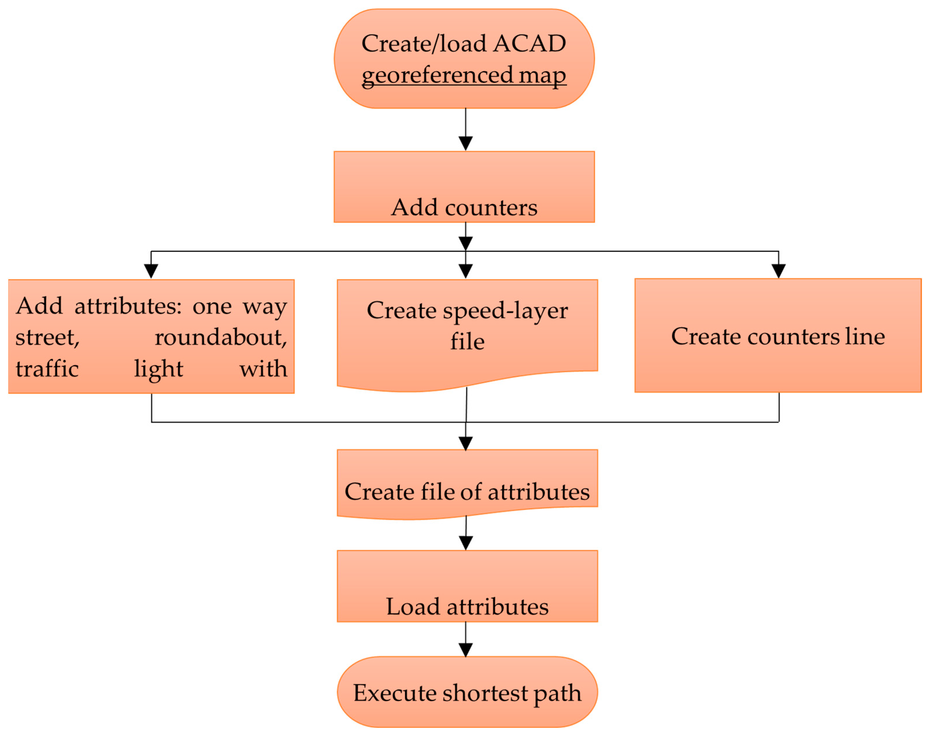
The application of Dijkstra’s algorithm to real-world problems requires additional effort in determining the parameters that will influence the edge weight values. Within a transportation network, it is possible to use travel time, driving speed, edge length, or any other parameter, depending on the desired output result. For the shortest path, time is the key parameter, and since it depends on other factors, it will be necessary to link them through preparatory steps.

In the Figure 2, the required sequence of steps is shown for determining the shortest vehicle route in a network with sparse traffic counters, measured by travel time.

As the first step, it is necessary to create or obtain a relevant map of the study area from available sources. Within the defined coverage area, traffic counters must be positioned based on their geolocation data.

Positioned counters serve as the foundation for executing the third operational step. This step defines traffic conditions in the network by creating one-way streets, roundabouts, and traffic signal controls. This process not only integrates physically existing elements into the map but also adapts their representation within the core computational part of the code to ensure unambiguous identification. Speed is defined at this stage by assigning an appropriate value to each street based on its hierarchical level and sorting them into a separate file. Additionally, street lengths are graphically added to the drawing for those segments where the impact of counters is considered unchanged.

The previously created attributes are then synthesized into a single file containing all necessary data for route calculation. Since these files are generated using specialized AutoLISP algorithms, they remain independent of the main code and do not affect the overall computation time, as they only need to be created once.

The final step involves loading the latest generated file into the computational Dijkstra code, where the route is calculated based on the selection of the start and end points and the time of day for which the route is being analyzed. If multiple routes need to be calculated, there is no need to reload the file, as the data it provides remain active within the drawing. The user is also given the flexibility to modify the endpoints and the calculation time, as needed.

4.2. Graph Edge Weights Determination

In the simplest case, the weight of an edge in a graph can be represented by its length. Given the structure of the urban traffic network, the length of the streets that form it satisfies this requirement, but the purpose and operation of the network itself necessitate the introduction of additional conditions. These relate to the unevenness of traffic speeds, the volume of traffic signals regulating the time distribution for street use, and the “interference” caused by other participants in performing the required maneuver. All of these factors can be evaluated in terms of the time required to execute them, thus affecting the overall result of the path selection.

Since all these factors are not independent of each other and are not strictly defined, they need to be reduced to the domain of the smallest deviation from the real situation when calculating the path. Furthermore, these factors are time-varying and can be observed at different levels, from minute-by-minute to annual intervals.

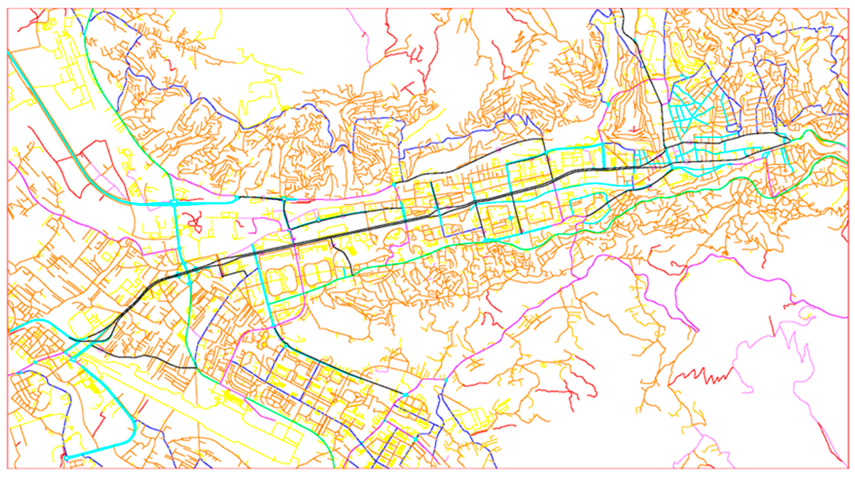
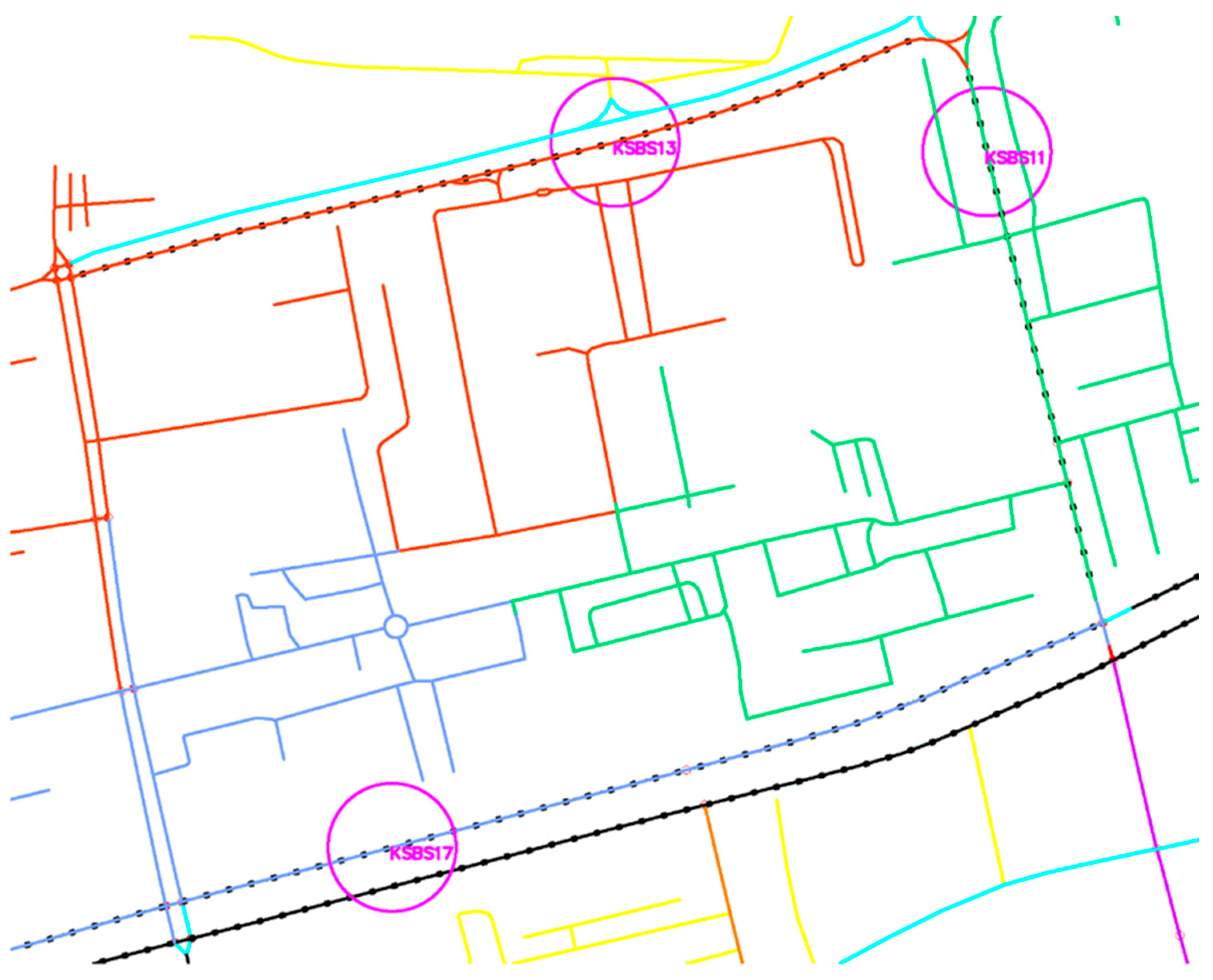
For an ideal solution, it would be necessary to achieve full coverage of the urban area with a service that would provide values for flow (Q), density (G), and speed (V) at every given moment in time, which is currently an unattainable task. The existing infrastructure, which in some way reflects the use of the traffic network, can be used to form a pattern that would be incorporated into the more detailed definition of street weights. For this purpose, a traffic counter network can be utilized, which, in addition to counting vehicles, also provides data on the speeds at which the counted vehicles were traveling. As a case study, this research focuses on the city of Sarajevo in Bosnia and Herzegovina, with its network of sparsely distributed traffic counters (Figure 3).

Obtaining the vehicle speed along a street is significant, because it eliminates the need to know the other two parameters (Q and G) as intermediaries in determining the speed, V. However, the network of traffic counters is not widely distributed in any area, so considering only individually located counters cannot provide the complete picture. Instead, the idea of this work is to define a zone where it can be assumed that the conditions are the same as those achieved at the counter, and such conditions can be used to determine the travel time on streets where the counter is not physically present. Regular users of the urban network use it based on their habits and experience, and they are the main factors behind the results obtained from the measurements. Transient urban traffic with a smaller volume can disrupt or affect the usual pattern.

Given that counters are generally placed on roads that have a greater tendency to attract traffic and, therefore, a higher traffic frequency, they can be viewed as fictitious movement targets where speed measurement is also carried out. Analogous to the goal, there must be sources, which are all streets that gravitate toward a counter, meaning that they direct traffic to higher-ranking roads. A street will gravitate toward the counter to which it has the shortest path.

4.3. Assignment of Maximum Speed Value to Streets

Solving the shortest path selection problem in the AutoCAD environment requires the prior preparation of an appropriate base. The road network can be created independently or downloaded from one of the available platforms, such as Open Street Map (OSM), which was used in this particular example. The most important factor is certainly the topology of the network and the classification of roads according to their functional rank, with each rank being assigned a maximum allowable speed value. In this study, 14 functional ranks are defined with a speed range from 30 to 110 [km/h]. Each street is created from a series of LINE entities in the appropriate layer. Depending on the geometry, the street can be composed of one or more connected LINE entities.

For the purpose of assigning speeds to each functional rank, an algorithm was created in AutoLISP programming language 01—speed layer pair. The idea of the algorithm is that by interactively selecting the layer in the drawing, which represents the functional rank, the user is offered the possibility of assigning a speed value in [km/h]. During the cyclic repetition through all layers, the recorded values are stored in a separate list, and after completion, the list is saved to a file. The file has a .TXT extension and is later loaded into other AutoLISP files. The advantage of this approach is that it is sufficient to create the values through the program code once, and they can later be changed directly in the file, as needed. Additionally, the file can also be created independently without using AutoLISP code, paying attention to the format, which is the layer name, separated by a TAB separator, and the speed value in decimal notation.

4.4. Creating One-Way Streets

The use of one-way streets in urban traffic organization is inevitable, either for the rationalization of space usage or to increase functionality. Therefore, this movement model needs to be established when selecting the shortest path in a graph. Dijkstra’s algorithm can also be applied to directed graphs, which is a realistic representation of a one-way street. Since a city is never entirely made up of one-way streets, the graph will represent a combination of both two-way and one-way traffic. A directed graph implies that movement is possible from node i to node i + 1, but movement from node i + 1 back to node i is prohibited. This principle must be adopted through the modification of the algorithm, restricting the nodes that can be visited based on the node from which the movement originates.

Since the entire network within the AutoCAD program is created from LINE entities, and each line has its start and end defined by group codes 10 and 11, it is impossible to establish a sequence of lines that would orient coordinates in the desired direction of movement. Additionally, it is possible that, at some nodes, only the ends of lines meet (with coordinates containing only group code 11) or the starts (the group code for all lines departing from the node is 10). This makes selection based on group code practically impossible.

The problem is overcome by using polyline entities, as they consist of a series of interconnected segments, where the end of one segment is simultaneously the start of another, allowing the definition of coordinates along which movement is possible or restricted. To edit this base segment, AutoLISP code 02—one-way street Dijkstra has been created. The idea of this code is based on the fact that a polyline is drawn along the line segment where one-way traffic occurs, starting where traffic enters the street and ending where it exits. This way, the allowed direction of vehicle movement matches the sequence of coordinates (from first to last) that make up the polyline entity.

Drawing individual polyline entities in AutoCAD is inefficient, as each vertex along the segment needs to be selected. To save time, the 02—one-way street Dijkstra code uses the concept of the shortest path between the starting and ending points of the street. If the part of the city with the one-way street is considered a graph, it is possible to find the shortest path between the start and end points of the one-way street. The code prompts the user to select the area (LINE entities) containing the requested segment, as well as the starting and ending points. The embedded Dijkstra algorithm searches for the shortest path between the specified nodes, considering only the edge lengths as weights. The speed of movement is not used as a parameter, as only the geometric condition of the street’s shape needs to be respected.

Depending on the geometry of the requested street and the number of selected lines, the calculated path may deviate from the one that should represent the one-way street (Figure 4). If the actual one-way street is marked as 1–2–3, the algorithm will give the shortest path marked in dark blue (1–3). For this reason, the user is presented with an option through a command line query to either accept the proposed path (command: accept the street) or correct it (command: exclude the edge at the first wrong turn). The correction involves selecting the segment (LINE) at the point where the proposed path first deviates from the correct one.

In Figure 4, this would mean selecting the brown line that exits from node 1 and goes towards node 3. A reselection of the area (to reform the graph) is not required; instead, the selected incorrect street is eliminated from the existing graph, and the calculation is repeated without it. The correction can be performed an unlimited number of times until complete alignment between the real state on the ground and the presentation in the graph is achieved (cyan line 1–2–3 in the figure). In the code, an automatic layer is created for the given line, in which the line is drawn, and through its name, it is invoked in the Lisp code in later steps. This layer is not allowed to be changed. The advantage of this labeling is that each one-way street is clearly visible, and any removal can be completed with the standard ERASE command. For creating very long streets to improve the efficiency of the algorithm, it is recommended to select graph edges using the WP or CP option, where it is possible to quickly select the required set and discard edges that clearly do not form the desired one-way street.

Although in a different form, a roundabout is essentially also a one-way street, so the same idea can be applied to its creation. The basic base in the AutoCAD drawing should consist of a series of short lines forming a circular shape, over which a one-way polyline should be drawn. Since the roundabout forms a closed contour, the previously created Lisp file for the one-way street has been partially modified and defined as 03—roundabout.

Essentially, the Lisp is automated to invoke the Dijkstra algorithm twice. The user is asked to select any two points on the roundabout, and since the direction of movement is always counterclockwise, the algorithm will first draw a path between the first and second selected points. The second call continues drawing in the same direction between the same points, drawing the missing segment to close the full circle. The layer, as well as the method of manipulating the drawn element, is identical to that described for the one-way street. The user is also given the option to accept the path or correct it by eliminating the “first wrong turn”; although, the likelihood of using this is very low.

4.5. Creation of Traffic Lights

The free flow of vehicles in the network is limited by the presence of traffic lights. As part of preparing the background, before calculating the shortest path, it is necessary to position them in space and determine their functionality in the program code.

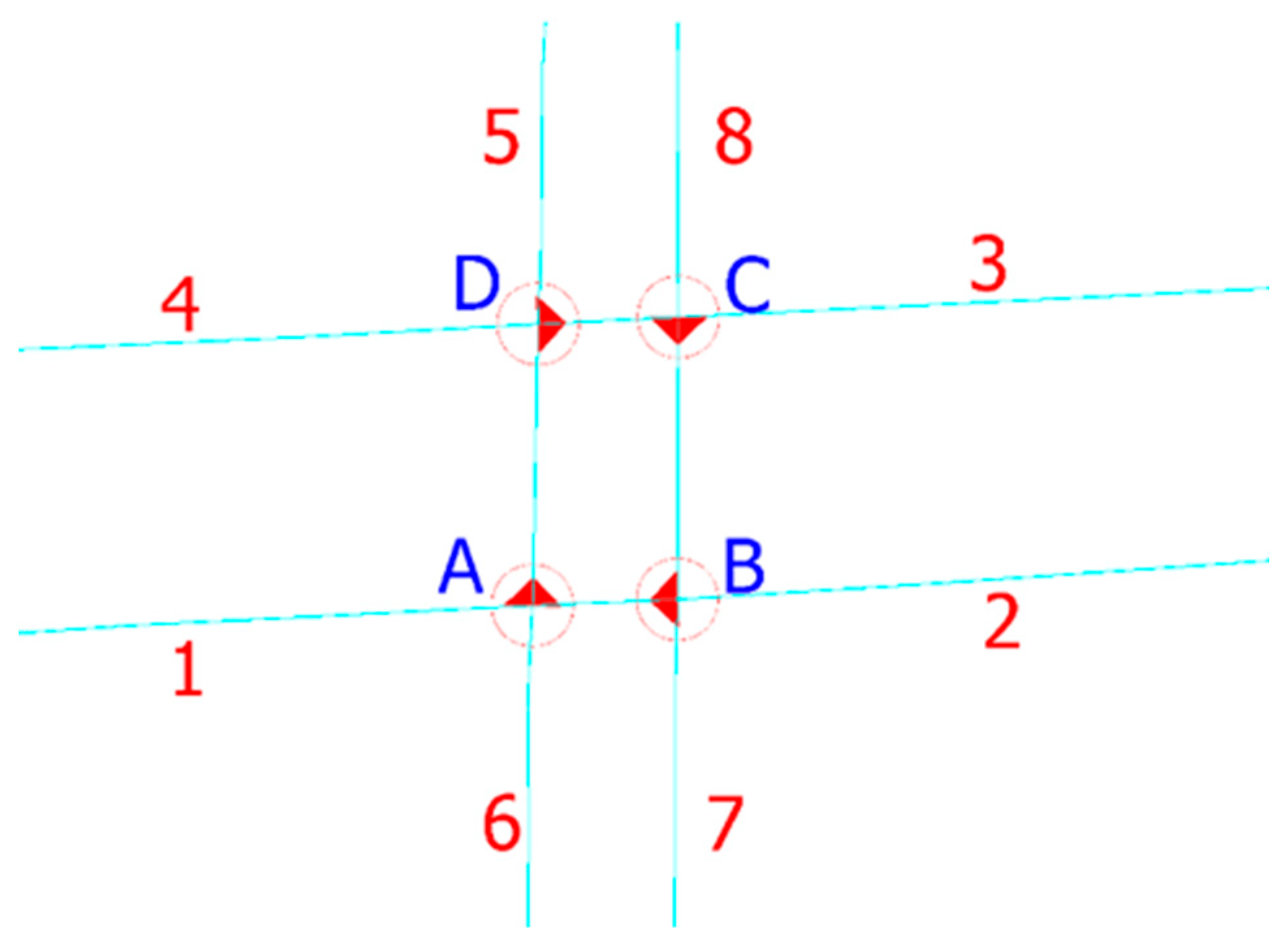
Considering the structure of the graph, where all operations take place at nodes, and the function of traffic lights, which, if present at an intersection, must physically exist at every direction and movement lane, a problem arises when transferring the real situation to the graph. If the traffic lights are at intersections where streets cross on a shared roadway for both directions, the traffic light can be defined as a single point at the intersection. Although, in real-world implementation, this means there are at least four units that control movement for each direction, in the graph, the appearance of just one element is sufficient to assign waiting time for each direction. In this work, the symbol for a traffic light is represented by a POINT entity with the layer name “traffic_signal”.

Intersections where directions are physically separated on independent roadways require a modification of the aforementioned solution. At such intersections, one-way streets intersect, and the allowed movement directions are 1–2, 3–4, 5–6, and 7–8 (Figure 5). The red points (POINT entities) marked with blue letters A, B, C, and D represent traffic lights, which are physically necessary for the intersection to function.

In addition to being physically present in the real network, traffic lights must also exist in the graph, but their function is limited depending on the maneuver the vehicle performs. In the case of a vehicle moving in the direction 1–2, the mandatory traffic light is the one at point A, as the vehicle must stop there regardless of which maneuver out of the possible three it wants to perform. A right turn allows the vehicle to continue in the direction 5–6 (direction 6–5 is not allowed) with only one potential stop at point A. Moving straight (direction 1–2), the vehicle would, according to the diagram, additionally have to comply with the timing conditions set by the traffic light at point B, which is unrealistic. Finally, the left turn maneuver implies that, from direction 1–2, the vehicle continues in direction 7–8, where traffic lights A, B, and C appear on the path, with only traffic light A being real. This scenario is not realistic in the actual network, so certain restrictions need to be introduced in the graph.

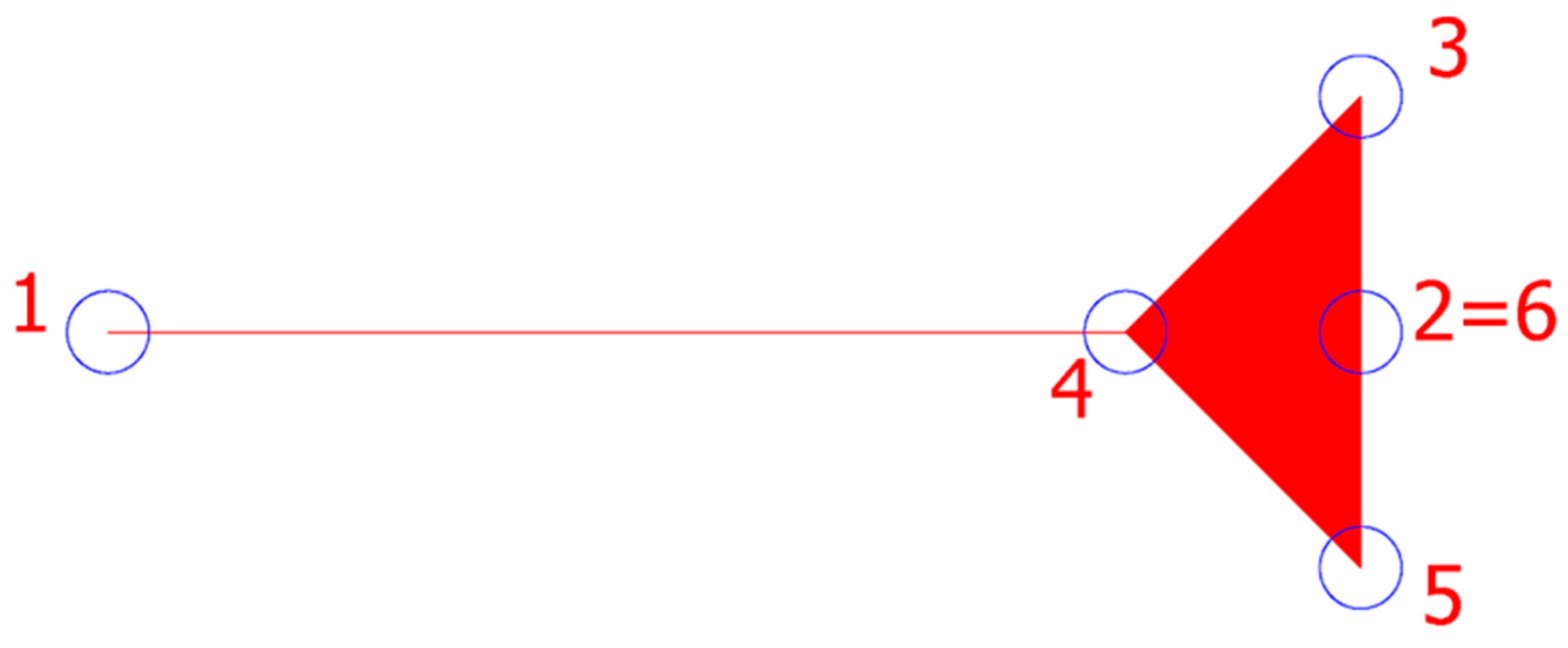
The restrictions are designed in such a way that the traffic light function is ignored in the Dijkstra algorithm if the vehicle comes from a direction that has been previously defined as eliminating. For this purpose, an AutoLISP code was designed in the file 04—traffic lights restrictions. The goal of the algorithm is to create a graphical marker that clearly defines from which side the traffic light is not usable. Since movement in the graph is defined through a node and searching its followers, the marker is designed to cover the entire line at the ends of which the node and its follower are examined. The marker is constructed as a closed polyline with six vertices, and for visibility in the drawing, the enclosed area of the contour is filled (Figure 6). The contour closes at vertex 6, which coincides with vertex 2. The blue circles in the image are added only as labels for the vertices of the polyline.

The marker, after calling the Lisp file, is placed by selecting the line that enters the traffic light, and it will be positioned so that point 2 corresponds to the point where the traffic light is located, while point 1 will be at the other end of the line leading to the traffic light. If, during the search for the shortest path, there is a need to examine a node marked here as 2 (or 6), such that it is reached from node 1, the waiting time at the traffic light will be set to 0. The manipulation of markers is such that they are added by calling the Lisp file and deleted using the AutoCAD command ERASE. A layer called TL_restriction is automatically created for the markers.

4.6. Position of Traffic Counters in the Network

Since the idea of the paper is based on utilizing the capabilities of traffic counters, it is necessary to clearly present them in the drawing. The position of the counters is constant and determined by coordinates, which are often an integral part of the traffic counting document [42].

As already emphasized, working in a graph requires that all elements used (which are mainly attributes that will participate in determining the weight of edges) are connected to the nodes or edges. In this work, counters are linked to the nodes of the graph, and their visual identification is represented by the MText object with the counter’s name inside a circle (circle object) (Figure 7), placed in the “counter” layer.

Although a point element, the counter in this work has a different relationship with the rest of the network. The values recorded by the counter are valid for the section before and after it, and it can be assumed that the same conditions will be represented over a longer section of the street where the counter is located. Since it is necessary to find the zone where the influence of the counter is felt, the problem is redefined. Instead of selecting streets that gravitate toward a single point, the streets that gravitate toward the linear element, which will be defined as the “counter line”, are identified.

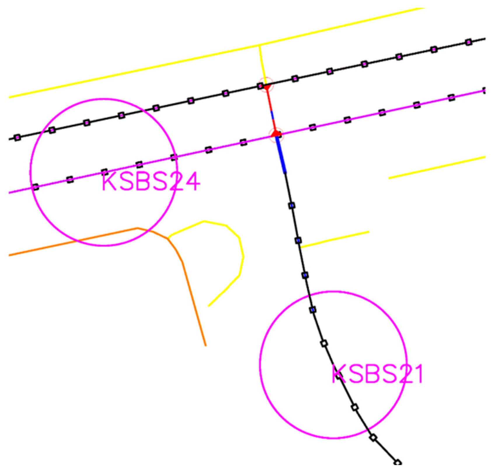
The length of the street where the conditions are identical to those at the counter can be determined through the hierarchical level of the streets. If the counter is positioned on a street that is connected at both ends to streets of a higher hierarchical level, the linear influence of the counter extends between these intersections. Figure 8 shows the intersection of a street hierarchically marked as tertiary (blue line, with counter KSBS21) and a secondary street (magenta line at counter KSBS24), noting that the red elements in the image are traffic light markers (Figure 6). As with other preparation elements, the method for marking this part of the line has been defined. In this case, the FENCELINE2 line type has been adopted as the marker, partly due to the symbolism of the line’s name and partly for practical reasons, as the overlap of multiple lines allows the type of line (street hierarchical level) represented by the FENCELINE2 line to be easily seen without further work. It is important to note that these lines do not connect at the same point but leave the shared intersection point as belonging to the higher-level street. The drawing of these lines has been resolved in the same way as the drawing of one-way streets, using the Dijkstra algorithm in the AutoLISP file 05—drawing counters.

Due to the purpose of the line it creates, a modification has been made in this Lisp, which relates to the name of the counter to which the line is connected. After drawing, the name of the counter to which the line belongs is attached to the polyline entity using extended entity data (EED). This allows each line entity that makes up the urban network to be identified with the original name of the counter whose influence extends to the given line through subsequent calculation steps.

If it happens that the streets with counters are of the same level, then the line of influence extends to their common intersection, with the note that the last point of one and the first point of the other must not overlap.

4.7. Determining Counter Belonging—Network Attributes

The previously created LISP files aimed to prepare the base in a format suitable for the main LISP file for calculating the shortest path. Given the specificity of the idea, where it is essential to know the position of each street in relation to the counter, it is reasonable to create a file that contains data about this belonging before the calculation. This way, the main program code would be freed from constantly recalculating data that are otherwise constant for a city. For this purpose, the AutoLISP file 06—network attributes (Supplementary Materials Section S1) was created. This file consolidates data about all previously mentioned and drawn elements in the drawing (one-way streets, traffic lights, traffic light restrictions, and speed limits on individual streets). The file is designed to generate an output .TXT file with all the relevant data, which are created once and later loaded into the main LISP file, as needed.

The first step is to load the file containing the functional classifications of streets and the speeds assigned to them. This allows the final .TXT file of attributes to associate the maximum speed at which vehicles are allowed to travel on each street. Additionally, the layer names from this file are used to create a selection set for all the edges of the graph. Streets will be identified during the calculation by their end coordinates and handle.

In the next step, all counter lines are selected through a section of the code, as follows:

(setq counter_street_SS (ssget “x” (list (cons 0 “LWPOLYLINE”) (cons 8 “counter_street”) ‘( -3 (“c_name”))))).

This selection implies that the counter lines must be entities of the LWPOLYLINE type and that the layer in which they were drawn is named counter_street. Since each counter line is assigned the name of the counter it corresponds to during drawing, the list with group code -3 points to the extended entity data associated with it, which is the counter name. By evaluating the part of the code after the selection, a list is formed, consisting of as many sublists as there are counters. Each sublist contains the counter’s name and the coordinates of the points on the counter line:

((“KSBS06” (6.53052e+06 4.85767e+06 0.0) (6.53053e+06 4.85768e+06 0.0)…) (“KSBS17” (6.53139e+06 4.85795e+06 0.0) (6.53138e+06 4.85795e+06 0.0)…).

According to the same selection principle, a list of one-way streets is created using a line of code that only takes those elements specified by the filter with group codes 0 and 8:

(setq ows_SS (ssget “x” (list (cons 0 “LWPOLYLINE”) (cons 8 “OneWayStreet”))))

The operations related to this part of the code create a list of grouped adjacent points of the one-way polyline in pairs, and then, the list is reversed using the reverse command, flipping each individual pair (each sublist) within the list. Since the one-way street is drawn so that traffic is allowed in the sequence of its coordinates, this reversal provides data in coordinate pairs where traffic is prohibited.

Another element drawn on the map, which is included in the attribute calculation through the selection set, is traffic lights with their corresponding filter elements with group codes 0 and 8, the final result of which is a list of coordinates, as follows:

(setq TL_SS (ssget “x” (list (cons 0 “point”) (cons 8 “traffic_signals”))))

Along with the traffic light, the restrictions on its usage are also selected.

(setq SEM_R_SS (ssget “x” (list (cons 0 “LWPOLYLINE”) (cons 8 “TL_restriction”))))

The output result of this is a list of sublists, each consisting of pairs of points 1 and 2 (markers in Figure 4). The appearance of any pair from this list in the decision-making process of the main path will eliminate the traffic light as a holding point.

The selection set is also used to load the streets, with the selection adjusted to those layers that are already present in the file where their speeds have been assigned, which was loaded at the beginning of the code, as follows:

(setq sel_LST (list))

(foreach lej list_lay_Vmax_f

 (progn

  (setq name_L (car lej))

  (setq lej_L (cons 8 name_L))

  (setq 4_lst (list (cons -4 “<AND”) (cons 0 “LINE”) lej_L (cons -4 “AND>“)))

  (setq sel_LST (append sel_LST 4_lst))

  )

 )

(setq sel_LST (cons (cons -4 “<OR”) sel_LST))

(setq sel_LST (append sel_LST (list (cons -4 “OR>“))))

(setq edges (ssget sel_LST))

The movement through the list lay_Vmax_f enables the identification of all used layers and the selection of the corresponding LINE entities. This eliminates the possibility of incorrect selection, and the extent of the elements covered is determined by the user through the offered selection scope.

By creating the edge set, all graphic elements relevant for participation in determining the shortest path are consolidated. In the following part of the code, for each individual edge from the selection set edges, the following elements are extracted: starting and ending coordinates (with group codes 10 and 11), layer, and handle. Indirectly, the maximum speed for each street is determined by searching the list of the first loaded file based on the street layer name. These parameters for each individual street are then searched in the previously defined restriction lists to form the list of followers for each point. During the examination of a street, it is important to note that the point with group code 10 will have a follower at point 11 and vice versa.

Pairs of end coordinates of lines (10–11 and 11–10) were checked for presence in the list of reversed one-way streets (prohibited direction), and if present, they were eliminated as possible segments for participation in the path. Individual points (both at 10 and at 11) were checked for coincidence with traffic lights and then for restrictions. If no traffic light is present at the intersection, the follower value is recorded as 0; where a traffic light is present, that value is 1. Additionally, for points found both in the traffic light list and the restriction list, a flag indicating the absence of a traffic light (0) is added. As a result of this part of the code, a list is formed where the sublists have the following structure:

((X_t Y_t Z_t)  ( (X_f1 Y_f1 Z_f1) Vmax₁ „HANDLE₁“ T_tl1) (( (X_f2 Y_f2 Z_f2) Vmax₂ „HANDLE₂“ T_tl2)…)

where:

• (X_t Y_t Z_t)—coordinates of the point being examined;
• (X_f1 Y_f1 Z_f1)—coordinates of the follower;
• V_max1—maximum speed on the street defined by the point being examined and its follower;
• “HANDLE₁”—the street defined by the mentioned points;
• T_tl1—presence or absence of a traffic light (0 or 1).

((6.53498e+06 4.85609e+06 0.0) ((6.53498e+06 4.85607e+06 0.0) 40.0 “AAA5” 0.0) ((6.53497e+06 4.8561e+06 0.0) 40.0 “B367” 0.0))

The previous part of the code aimed to systematize and sort the attributes into the required form, which are clearly visible to the user on the drawing. In the next segment, a calculation that uses all the attributes is necessary in order to determine the influence zone of each counter, the meaning of which will be graphically explained in the following part of this paper.

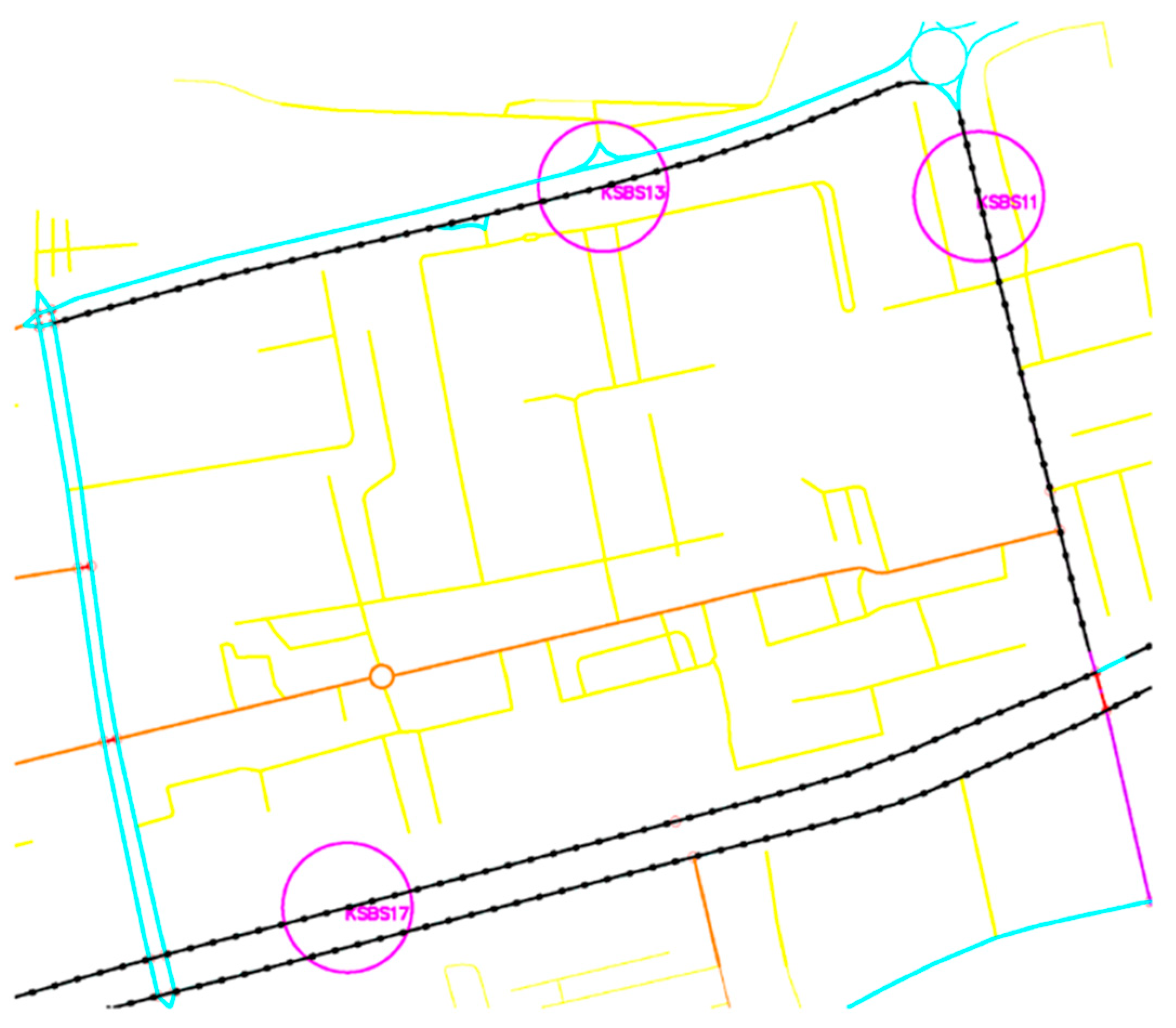
Figure 9 shows a part of the city zone of Sarajevo bordered by secondary and tertiary streets, within which there are service (yellow) and residential (brown) streets at the functional level. On the outer edges are the counters KSBS11, KSBS13, and KSBS17. Each counter is assigned a counter line in which the same characteristics as those on the counter itself are assumed and marked with the FENCELINE2 object. The same characteristics refer to the achieved (measured) driving speed and the number of vehicles across the entire marked area. In each calculation, it is necessary to identify the maximum speed of vehicle movement on the street where the counter is located. In the network area shown in Figure 10, the maximum speeds are 60 km/h for KSBS11 and KSBS17 (secondary rank) and 50 km/h for KSBS13 (tertiary rank).

The capabilities of the counters are numerous, but for this work, the average measured vehicle speed during a one-hour time interval has been adopted.

The idea used in this paper is based on determining the distance from each node in the network to the nearest counter line, with the assumption that the prevailing traffic conditions from the counter spill over into the coverage area. This approach somewhat resembles determining the shortest path for all pairs (Floyd–Warshall algorithm), but since the goal (the counter line) is already known, and the mutual distances between nodes that do not lie on that line are not needed at all, a different approach has been devised.

In the initial step of the algorithm, the counter line is considered as the source of movement, and a distance of 0 is assigned to each point of every line. In the next step, the algorithm finds all first neighbors connected to the counter line by a line element, calculates their distance as the length of the line element, and assigns the calculated value to the nodes (endpoints of the line). The algorithm repeats this process for each first neighbor of each counter line, placing the visited neighbors in a separate list. The purpose of the list is for the calculation to start again from its members, searching their first neighbors. The list is temporary, and after one pass through all the members, it is cleared and populated with newly examined nodes.

After the first step is completed, the process repeats by finding the first neighbors of the already calculated points, calculating the distances between them (also as the lengths of the line elements), but this time, the value of the distance recorded at the node is the sum of the distance to the current point and the calculated length of the line element (the procedure is the same as in the Dijkstra algorithm).

The purpose of determining the belonging to the counter is to assess the conditions prevailing on individual streets, and therefore, the results of the belonging must be linked to the streets, not just the nodes. For this purpose, in addition to the node, which is the main element for the calculation, all calculated values are also linked to the handle of each street in the code. Since the output result is a file that needs to be loaded into the main Lisp, handle is the best option for storing all the data associated with the element that needs to be processed.

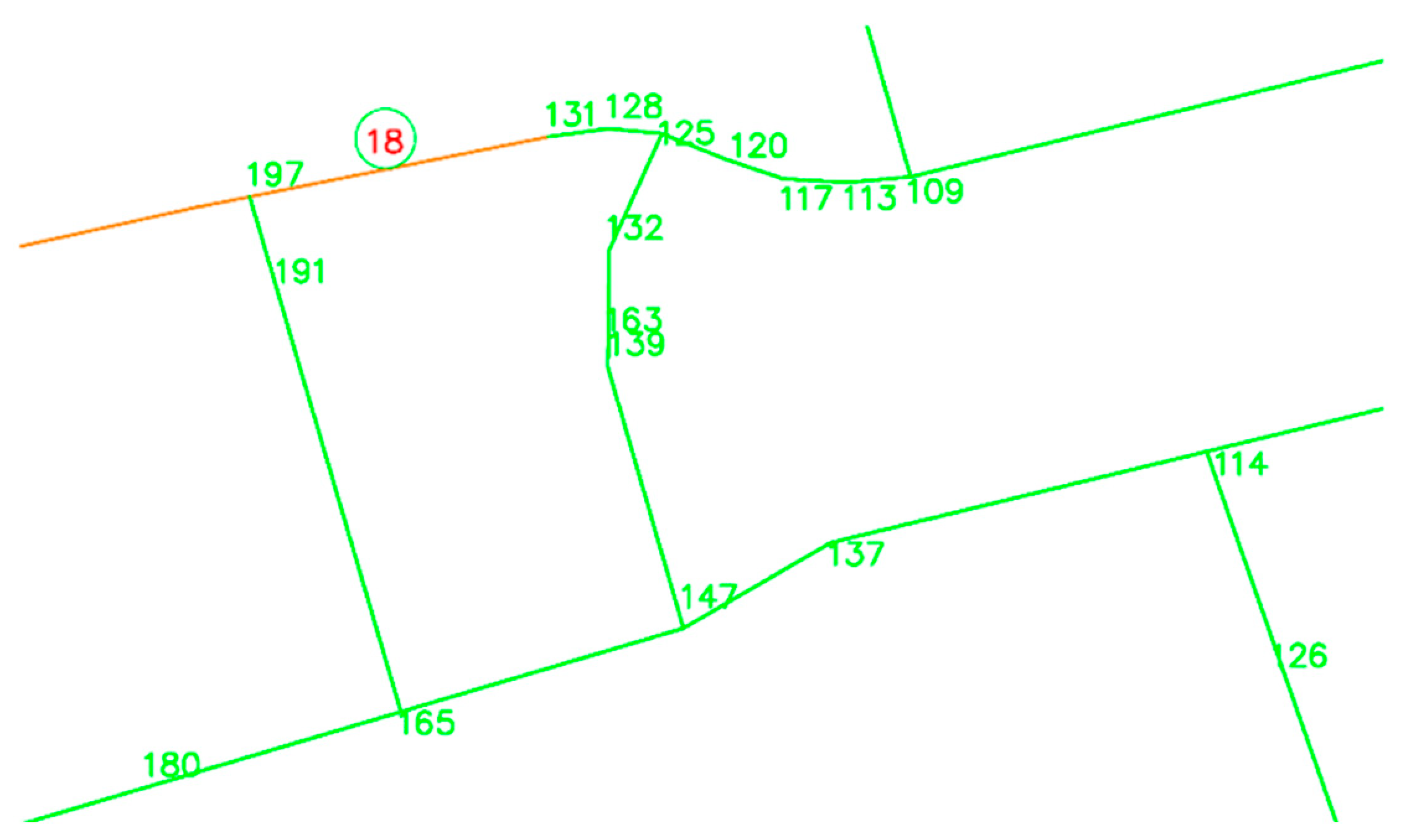
The algorithm for determining the nearest counter also relies on the BFS principle, in which one level is examined, and only after completing the processing does it move on to the next. Therefore, the length values at individual points depend on the number of lines through which the observed point is reached. As with the Dijkstra algorithm, if the calculation determines that a point can be reached by a shorter path than the current one, the shorter path is accepted. In Figure 10, all green paths start at the same point (a part of the city in Figure 9), but due to the configuration, unrealistic values are shown. The distance of 197 meters will certainly be replaced by the sum of 131 + 18 = 149 m at the marked node. What is important to note is that after replacing 197 with 149 m, the distance at the node currently recording a value of 191 will also change. Since the length of the line connecting 191 with 197 is 6 m, in the next iteration of the algorithm, this node will change from 191 to 149 + 6 = 155 m. This process repeats, as long as there is a possibility of obtaining a shorter distance.

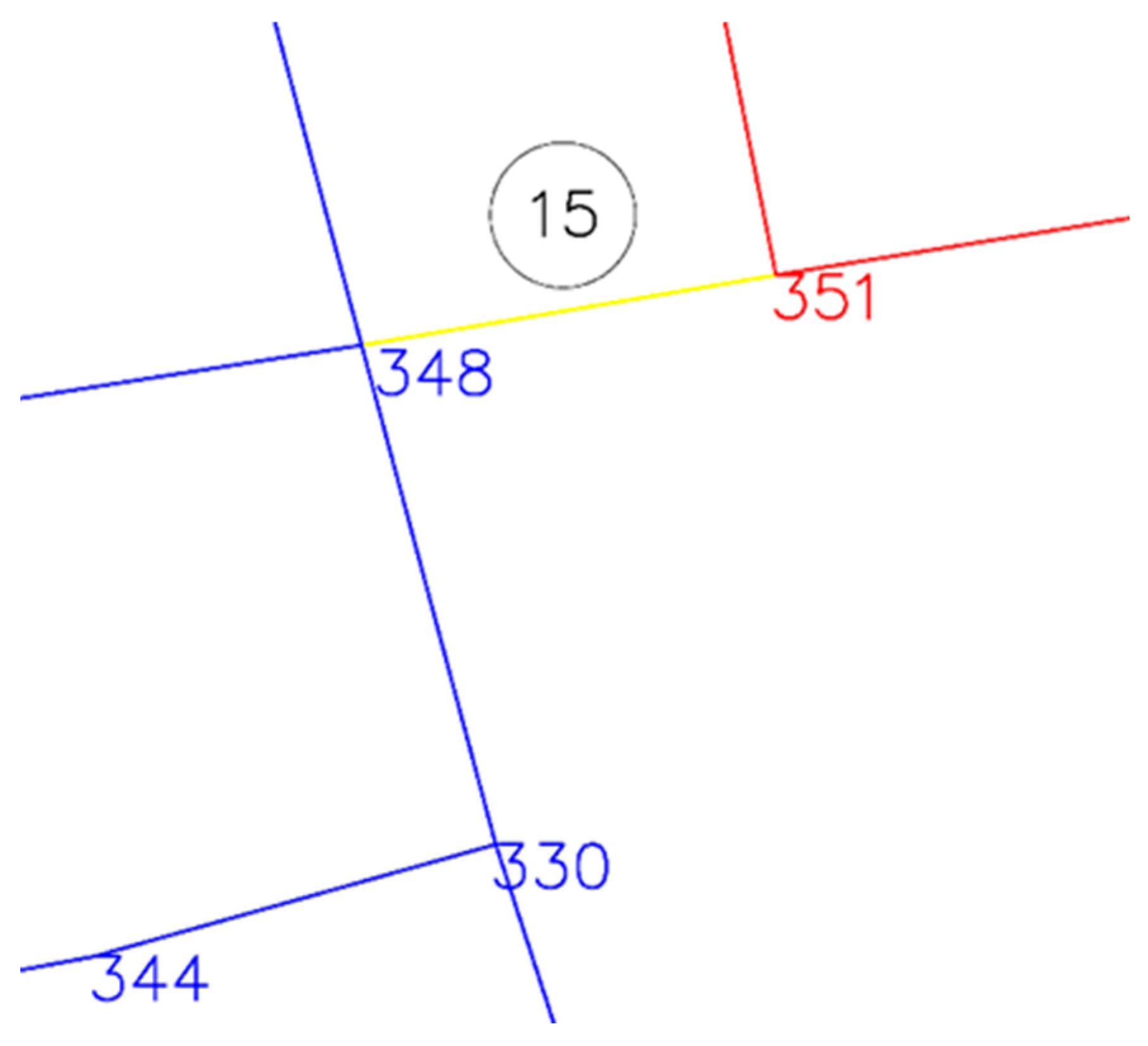
As long as the changes in distances are within the same counter, there is no issue with unclassified streets. For the situation in Figure 11, a special part of the algorithm has been designed. Observing the values 351 + 15 > 348 and 348 + 15 > 351, neither of the neighboring nodes of the blue and red paths will change their values. Therefore, a condition has been added to the algorithm that checks the total distance of each individual handle. For streets on the boundary, the smaller value of the distance to cross them is adopted, which, in the given example, will be 348 + 15 = 363, placing this handle in the blue zone of influence. 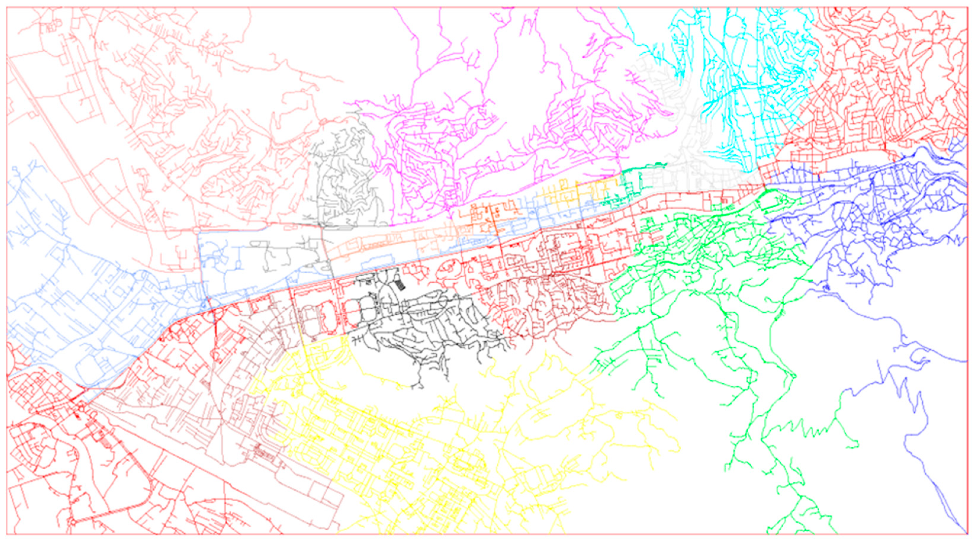The final form of the division of the selected part of the city from Figure 9 is shown in Figure 12, while the division of the entire considered urban area is presented in Figure 13.

As the final result, file 06—network attributes provides a list whose sublists have the following form:

((X_t Y_t Z_t)  ( „Counter_name₁“ Vmax₁ „HANDLE₁“ T_tl1) ( „Counter_name₂“ Vmax₂ „HANDLE₂“ T_tl2) )

where:

• (X_t Y_t Z_t)—coordinates of the point being examined;
• “Counter_name₁”—the name of the counter to which “HANDLE₁” belongs;
• Vmax₁—the maximum speed on the street “HANDLE₁”;
• “HANDLE₁”—the handle of the street;
• T_tl1—the presence or absence of a traffic light (0 or 1).

((6.53253e+06 4.8569e+06 0.0) (“KSBS05” 40.0 “9807” 0.0) (“KSBS05” 40.0 “982A” 0.0))

The final list is written to a .TXT file, with each sublist representing one line. It only needs to be calculated once and loaded, as follows:

6528182.225 4856482.834 0.000  KSBS23 40.0 B9A2 0  KSBS23 60.0 10CF9   0 6528174.893 4856482.581 0.000  KSBS23 40.0 B9A3 0   6528169.513 4856482.937 0.000  KSBS23 40.0 B9A4 0   6528152.019 4856492.507 0.000  KSBS23 40.0 B9AC 0  KSBS23 40.0 112E9   0 6528155.642 4856489.189 0.000  KSBS23 40.0 B9AC 0  KSBS23 40.0 B9AD   0 6528161.449 4856484.847 0.000  KSBS23 40.0 B9AD 0  KSBS23 40.0 B9AE   0 6528168.135 4856475.965 0.000  KSBS23 40.0 B9AF 0   6528383.578 4856201.326 0.000  KSBS22 40.0 B9B0 0  KSBS22 40.0 BE70 0

4.8. Determining the Shortest Path in a Graph

By creating a TXT file with the city’s attributes, a condition was established for running the Lisp file that contains the code for determining the shortest path. The shortest path is chosen based on the least amount of time spent traveling between the selected points. The code starts by asking the user for the time of day when the path is to be determined.

(setq HOUR_day (getreal “\nInsert the hour of the day for which the minimum route is required: ”))

The execution continues by loading the file with attributes and creating a list in the same format in which they were recorded, replacing the handle values with the coordinates of the opposite end of the line in relation to (X_t Y_t Z_t). It is important to note that all parameters, except for (X_t Y_t Z_t), can be read from the .TXT file with their actual values, while the point (X_t Y_t Z_t) is recorded in the file with three decimal places and, as such, cannot be identified with any existing endpoint of the graph’s edges. This is due to the difference in numbers after the third decimal place, which automatically classifies it as a new coordinate. Since each handle is in the same row as (X_t Y_t Z_t) and carries the exact coordinates of its follower, which is significantly different from (X_t Y_t Z_t), the point with the smaller deviation from (X_t Y_t Z_t) is recorded in the sublist instead of (X_t Y_t Z_t). The file loading process creates the GRAPH_PT list.

In the second step, the code requires loading the data collected from the counter. Since the collected data correspond to a time interval of one hour, it is necessary to prepare a .TXT file before loading, in which the average values of the measured speeds and the time they were measured will be written, following this format:

Counter-KSBS03 Vmax = 60 [km/h] 0  46 1  48 2  50 3  50 … 21  40 22  42 23  44 Counter-KSBS04 Vmax = 60 [km/h] 0  37 1  37 2  38 …

At the end of the loaded file, a list lst_C-HO-Vsr is created, whose sublists are

(“KSBS03” 60.0 (0.0 46.0) (1.0 48.0) (2.0 50.0) (3.0 50.0) (4.0 49.0) (5.0 50.0) (6.0 50.0) …)

With each counter’s name, the value of the maximum speed on the street where it is located is also added, and the measured speeds are recorded over a 24 h period.

The user is also prompted to select the starting and ending nodes of the path, or to select the line on which the specified node is located at its closer end. Considering that the shortest path search is a process that requires repeated iterations and depends solely on the selection of the end points, if there are no changes in the complete set of attributes loaded through the first two files, it is sufficient to load them only once. At the beginning of the code, the user has the option to choose whether to load the attributes or not via the following prompt:

(initget 1 “Y/N”)

(setq query (getkword “\n Load new attribute data <Yes or No>”)).

The next steps involve applying Dijkstra’s algorithm with modifications adapted to the ideas used in the previous work. First, lists of examined nodes and lists of reached and examined nodes are created. Unlike the original algorithm, the starting node is placed in the examined nodes, while the list of reached and examined nodes is empty. The distance value assigned to the starting node is 0.

By selecting the shortest value among the examined nodes, the algorithm faces no dilemma, since only one number is provided, the smallest possible (0). The purpose of this deviation from the original algorithm is to eliminate a condition that would have to be written only for the first node, met once, and checked on every loop iteration, knowing it would not be met again.

After the selection, the examined node (coordinates) is added to the list of reached and examined nodes and then deleted from the list of examined nodes. These two lists, which cannot contain the same nodes, have the same structure. They consist of sublists, which include the following:

((coordinates of the node with the shortest distance) (coordinates of its predecessor) shortest distance)).

This simplifies the reconstruction of the path from the last node to the first one, which is completed at the end of the algorithm. By setting the end node as the starting point, its predecessor and the distance to reach it are automatically identified in the list. Through an iterative process, the path continues back to the start node.

By selecting the coordinates of the node with the smallest distance, followers are determined by searching the GRAPH_PT list for the required point. Since the coordinates of the points are given as the first item in the sublist in this list, the ASSOC command is sufficient to retrieve all followers with their corresponding attributes. Among these followers is the node from which the current one was reached, so it is not considered as a potential for further progression.

Since the graph in question represents a traffic network, it is necessary to incorporate conditions that influence its operation. Knowing the followers is a necessary, but not sufficient, condition. Since the desired path is based on the shortest time spent driving, the type of maneuver (straight, left turn, right turn) is determined based on the position of the follower in relation to the incoming direction. If the achieved speed is equal to the maximum allowed speed, the assumption is that the flow is free of obstructions, and the maneuver will take the base time values, such as straight 3 s, right 5 s, and left 10 s [43,44,45,46].

The maneuver time assumes a reduction in speed to an acceptable value for executing the maneuver and adjusting to the obstacle that the intersection itself represents. If the driving speed during the observed hour is lower than the maximum, the difference between the maximum allowed speed (V_max) and the minimum speed recorded on the counter (V_min) needs to be found. This interval is considered the operational range and is assigned boundary values of V_max = 0 and V_min = 1. Each examined speed will also have its value within the range of 0–1, which is multiplied by the base maneuver values and added to them. This covers the assumption that arriving at a lower speed means higher traffic congestion and the need for more time to execute the maneuver.

To determine the type of maneuver, the following sign value was used:

$$tg{\displaystyle \frac{(\alpha -\beta )}{2}}$$

(8)

where:

• α—the angle formed by the positive X-axis and the line from the predecessor of the examined node to the examined node;
• β—the angle formed by the positive X-axis and the line from the examined node to the successor.

A positive sign of the expression implies that the successor is on the right side, while a negative sign indicates that the successor is on the left, which determines the type of maneuver. This condition, with certain adjustments, is applied to intersections with both four and three directions, as well as to the junction of two lines that maintain the continuity of the street.

After resolving the geometric conditions, the total travel time to each successor is calculated. The total time will be the sum of the time spent reaching the current point and the time needed to travel from the current point to the successor. The time from the current point to the successor is given by:

$$t_f=t_d+t_{tl}+t_m$$

(9)

where:

• t_d—travel time along the line (street);
• t_tl—time lost if a traffic light is present;
• t_m—maneuver time (straight, right, left).

For the time to be accounted for in the total path, which depends on encountering a traffic light, the duration of the red light for one direction of travel is previously defined. For this work, it is assumed to be 45 s [33]. When a vehicle arrives at the traffic light with speed V_max, it is assumed that traffic is not congested, and the waiting time is 0 s. For V_min, the previously assumed time of 45 s is taken. When the vehicle arrives at the traffic light with the tested speed, the waiting time will be equal to the product of the speed coefficient from the mentioned range of 0–1 and the total waiting time.

The value of t_d depends on the applied driving speed and will be determined through the following formula:

$$t_d={\displaystyle \frac{3.6\times L_L}{V_d}}$$

(10)

where:

• L_L—length of the line between the current node and the follower [m];
• V_d—driving speed [km/h].

Driving speed is a parameter determined depending on which counter the considered street belongs to. With the idea that the conditions of the counter spill over to the covered zone, it is assumed that the speed on the street will decrease in the same manner as it does at the counter. Based on the adopted calculation time (the hour of the day), the ratio of the measured and maximum speed at the corresponding counter is calculated, as follows:

$$Kh={\displaystyle \frac{V_{h,c}}{V_{\max ,c}}}$$

(11)

• V_h,c—driving speed measured at the counter during the specified hour;
• V_max,c—maximum driving speed on the street where the counter is located.

The product of the similarity coefficient (Kh) with the maximum driving speed on the considered street (V_max,str) will give the driving speed, as follows:

$$V_d=K_h\times V_{\max ,str}$$

(12)

All the parameters needed for the calculation are easily accessible from the previously created files loaded into the main code.

The algorithm repeats the process until the final node (end) is found among the reached and examined nodes. Since this list also contains nodes that are not on the path, the aforementioned predecessor search procedure from end to start will provide the complete path, recorded in the form of a list and graphically represented as the polyline entity. Also, besides the graphical representation, the user is provided with travel time, the number of nodes on the path, the number of examined nodes, and the algorithm’s execution time.

The program code for calculating the path 07—Dijkstra shortest path is given in Supplementary Materials Section S2.

5. Analysis of Results

The algorithm was applied to data from the city of Sarajevo (Figure 4), and to evaluate its performance, a comparison was made with the values provided by the Google Maps service. The base map was obtained from the OSM service, supplemented with the necessary missing line elements and data required for calculations in the main program code. The described program codes created in AutoLISP were used as tools for this supplementation.

In Sarajevo Canton, which is a larger territorial and organizational unit, a total of 29 counters are distributed, while, within the city zone, there are 20 counters, the results of which were used in this study. The base map consists of 46,497 lines (graph edges), which, according to their topology, provide 44,301 nodes within an area of 11.8 km × 6.5 km. Nodes are created by connecting at least two and no more than five lines. They are divided into fourteen functional categories with corresponding speeds, as shown in

Table 1. Functional rank of streets.

Functional Rank	Vmax [km/h]
secondary_link	40.000
unclasified	40.000
trunk	80.000
living_street	30.000
motorway_link	70.000
secondary	60.000
track	40.000
service	30.000
tertiary	50.000
residental	40.000
primary	60.000
primary_link	40.000
motorway	110.000

.

Table 2. Results of the Dijkstra algorithm.

Path	Hour of the Day	Path Length [m]	Examined Reached Nodes	Nodes at the Path	Driving Time Dijkstra [min]	Algorithm Running Time [s]	Driving Time GM [min]
1	13	2300	7153	138	8	25	9
2	13	1680	1964	110	5.6	7	6
3	14	4571	18,781	200	11.5	53	11
4	23	3570	7529	132	8.9	27	8
5	23	2651	6889	129	6.2	21	6
6	23	2700	7327	188	7.5	21	9
7	23	4183	33,369	245	15.4	259	14
8	23	1400	2881	87	4.6	4	5
9	11	9931	38,689	337	23.5	376	24
10	11	2088	2973	108	5.5	4	6

shows 10 results of randomly selected paths within the subject map. The checks were performed at different times of the day. Given the availability of the Google Maps service, which provides real-time data on the most time and spatially optimal paths, the results were compared with each other. Figure 14 Path 1 Dijkstra algorithm displays Path 1 from Table 2 as the output result of the algorithm, and Figure 15 Path 1 Google Maps shows the corresponding path in Google Maps. The difference in achieved times is 11% compared to the reference value.

Given the Olympic history of the city of Sarajevo, Path 1 was chosen to connect the base of the mountain where the bobsleigh competition was held with the Olympic Museum. In the total sample tested, the root mean square error between the Dijkstra driving time (Y_i) and the GM driving time (Y_p) was RMSE = 0.85, according to Equation (13).

$$RMSE=\sqrt{{\displaystyle \frac{\Sigma {\left(Y_i-Y_p\right)}^2}{n}}}$$

(13)

6. Conclusions and Recommendation for Further Research

The selection of the shortest vehicle route in an urban network has significant applications in traffic planning from the perspective of traffic management authorities, as well as in increasing efficiency for users. The proposed solution primarily aims to regulate the management of the most flexible and least predictable form of urban traffic.

The infrastructure required to accurately identify participants, process data on their movement, and display output results in real time demands a large amount of resources, even in less populated areas. To address this, the proposed model offers a solution utilizing relatively easily accessible data sources in the form of traffic counters, which are essential for any serious daily traffic management. The data obtained in this way, primarily referring to vehicle speed, serve as secondary information compared to the primary function of the counters, yet they provide a solid starting point for solving the given problem.

Although a traffic counter has a relatively small physical range of influence (limited by its equipment), it can be considered a representative sample that reflects the usage of all streets whose topology directs traffic toward the given area. This approximation provides insight into both the spatial impact and the dynamic characteristics of traffic. The majority of urban movement consists of already established routes, meaning their “footprint” in any given area does not significantly deviate from what is recorded by the counter.

Since the measured data are organized according to specific time intervals, the overall pattern can also be analyzed from that perspective. The advantage of this approach over existing ones is the ability to predict the optimal route for any time of day. This allows infrastructure managers to identify high-occupancy sections in advance and address “bottlenecks”. A certain degree of deviation from the reference level is acceptable, considering the level of approximation, as well as the fact that the obtained routes in shape correspond to the reference ones. Additionally, the advantage of using traffic counters is that, with relatively minimal resources (as the traffic counter network it-self represents), data can be collected for a significantly larger area.

The choice of the AutoLISP programming language and its application within the AutoCAD environment enhances the range of available tools for efficiently solving the given traffic management problem, while also allowing for easy manipulation through custom-written algorithms. This enables the flexible creation of networks with any topology, making the tool applicable to any urban environment with an established network of traffic counters.

The adopted model could be improved in the future by changing the set of input data, which would involve adopting speed measurement intervals of 5 to 15 min instead of the proposed 60 min. This would provide the infrastructure manager with a better insight into traffic fluctuations during the busiest hours of the day. Additionally, the study could be expanded and divided into different time intervals, such as seasons or workdays and weekends, allowing the manager to differentiate the solutions used according to the considered time period.

Beyond planning the physical distribution of traffic, research could also focus on predicting environmental impacts by estimating pollutant emissions and noise levels.

Also, future work could focus on determining vehicle loads due to road gradients and, thus, additionally modeling the weights of graph edges.