AASNet: A Novel Image Instance Segmentation Framework for Fine-Grained Fish Recognition via Linear Correlation Attention and Dynamic Adaptive Focal Loss

Abstract

Smart fisheries, integrating advanced technologies such as the Internet of Things (IoT), artificial intelligence (AI), and image processing, are pivotal in enhancing aquaculture efficiency, sustainability, and resource management by enabling real-time environmental monitoring, precision feeding, and disease prevention. However, underwater fish recognition faces challenges in complex aquatic environments, which hinder accurate detection and behavioral analysis. To address these issues, we propose a novel image instance segmentation framework based on a deep learning neural network, defined as the AASNet (Agricultural Aqua Segmentation Network). In order to improve the accuracy and real-time availability of fine-grained fish recognition, we introduce a Linear Correlation Attention (LCA) mechanism, which uses Pearson correlation coefficients to capture linear correlations between features. This helps resolve inconsistencies caused by lighting changes and color variations, significantly improving the extraction of semantic information for similar objects. Additionally, Dynamic Adaptive Focal Loss (DAFL) is designed to improve classification under extreme data imbalance conditions. Abundant experiments on two underwater datasets demonstrated that the proposed AASNet obtains an optimal balance between segmentation performance and efficiency. Concretely, AASNet achieves mAP scores of 31.7 and 47.4, respectively, on the UIIS and USIS dataset, significantly outperforming existing state-of-the-art methods. Moreover, AASNet achieves an inference image recognition speed of up to 28.9 ms/per, which is suitable for practical agricultural applications of smart fish farming.

1. Introduction

Smart fishery aquaculture is becoming the core direction of modern fisheries, aiming to achieve intelligence, automation, and informatization in fishery production through the deep integration of the Internet of Things (IoT), big data, and artificial intelligence technologies [1]. It allows for real-time monitoring of water quality indicators (e.g., pH, dissolved oxygen, ammonia, and nitrogen content) and enables automatic adjustments to the aquaculture environment to support the healthy growth of aquatic organisms. This approach also reduces labor costs, improves production efficiency, and enhances product quality [2]. Furthermore, smart fisheries minimize feed waste and pollutant discharge, protect the ecological environment, and promote the sustainable use of fishery resources through precise feeding and water quality management [3].

Instance segmentation [4,5,6], as one of the key tasks in computer vision, has made significant progress. The goal of instance segmentation is to assign each pixel in an image to a specific object instance, enabling precise recognition and segmentation of different objects within complex scenes. With the growing demand for automation and precise monitoring in aquaculture, the deep learning community has increasingly focused on the development and application of underwater vision tasks. Underwater vision involves the analysis and interpretation of underwater images, which is critical for robotic vision systems and the navigation of autonomous underwater vehicles. In agricultural fish farming, underwater image instance segmentation plays a pivotal role in effectively identifying and detecting fish and their behaviors, thereby assisting in monitoring the farming environment and optimizing management decisions. This process is essential for applications such as health monitoring [7], population management, and stocking density control in aquaculture. Despite its significance, agricultural underwater image instance segmentation faces numerous challenges, making this task particularly complex.

Firstly, variations in lighting and color in underwater scenes significantly affect the accuracy of image segmentation. Due to the scattering and absorption properties of underwater light, objects at different depths show varying colors and brightness levels [8]. These factors lead to inconsistencies in feature representation, making it difficult to maintain semantic consistency in the segmentation model under changing lighting conditions [9]. This inconsistency poses a major challenge to accurate object recognition and differentiation. Additionally, objects at greater depths appear darker and less distinguishable due to light scattering, further complicating the segmentation process. The changes in the appearance of objects, driven by fluctuating lighting conditions, result in a notable decrease in the performance of segmentation models, which often struggle to adapt to the dynamic nature of underwater images.

Secondly, underwater image data are often highly imbalanced, which presents another critical challenge. In many natural underwater environments, large schools of fish tend to gather around coral reefs or other structures, resulting in a much higher number of fish instances compared to other objects such as plants, rocks, or debris. This uneven distribution of object categories creates a skewed training dataset, where the model encounters an overwhelming frequency of fish instances in contrast to less common objects. As a result, the model prioritizes the detection of more frequent objects while neglecting or misclassifying rarer ones. This data imbalance negatively impacts segmentation performance, especially for less frequent objects, as the model struggles to learn to recognize them accurately. The problem becomes more complex when infrequent objects appear alongside more common ones in the same frame, further challenging the model’s ability to correctly segment these rare instances.

In this work, we propose a novel deep learning segmentation model, defined as the AASNet (Agricultural Aqua Segmentation Network), which incorporates a Linear Correlation Attention mechanism and a Dynamic Adaptive Focal Loss, that is specifically optimized to address challenges such as lighting variations, complex backgrounds, and extreme data imbalance in underwater scenes. The model’s performance has been extensively evaluated on the UIIS [8] and USIS10K [10] datasets. To summarize, our main contributions are listed as follows:

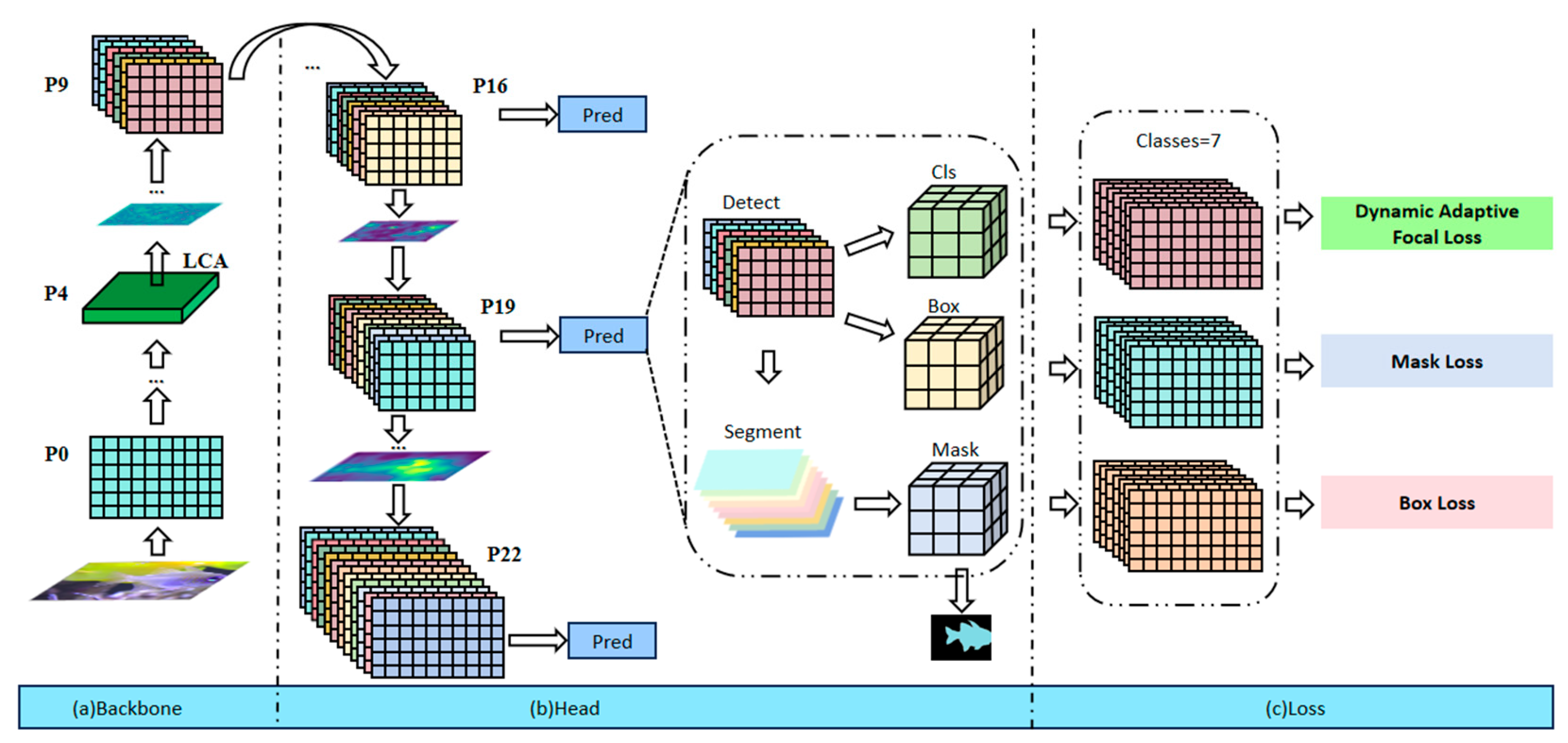
• We design a novel Agricultural Underwater Image Instance Segmentation Model, AASNet, which integrates detection and segmentation functions. This model is specifically optimized to address the challenges of lighting variations and extreme data imbalance in underwater scenes.
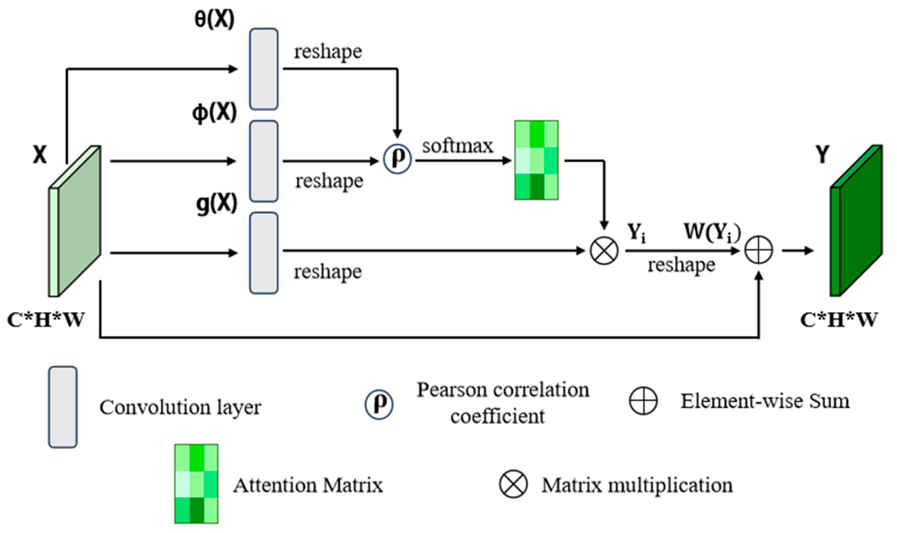
• In AASNet, we introduce the Linear Correlation Attention (LCA) mechanism and a dynamic adaptive loss function. The LCA mechanism captures feature correlations, enhancing the model’s ability to adapt to variations in lighting and complex backgrounds. At the same time, the dynamic adaptive loss function addresses the issue of data imbalance, improving classification accuracy and ensuring that the model maintains high performance across diverse underwater scenarios.
• Our method achieves state-of-the-art performance on the UIIS and USIS datasets, surpassing current mainstream methods in accuracy, parameter efficiency, and inference speed. The experimental results demonstrate that AASNet excels in handling complex underwater scenes, showcasing its superior performance.

The remainder of the paper is organized as follows: Section 2 reviews the related work in underwater image instance segmentation, discussing key approaches and their limitations in addressing the challenges posed by underwater environments. Section 3 presents the methodology behind AASNet, detailing the innovative components of the Linear Correlation Attention mechanism and the Dynamic Adaptive Focal Loss. Section 4 outlines the experimental setup and results, comparing AASNet’s performance with state-of-the-art methods on the UIIS and USIS10K datasets. Section 5 discusses the results, emphasizing the advantages of AASNet and its potential applications in smart fisheries, and provides suggestions for future research directions.

2. Related Work

2.1. Vision Instance Segmentation Technology

Current instance segmentation methods fall into two categories: two-stage and one-stage approaches. Two-stage methods, like the classic Mask R-CNN [5], first generate region proposals or bounding boxes, followed by RoI pooling to align features and predict pixel-level masks. PointRend [11] builds on Mask R-CNN by adaptively selecting key points to recover fine details, generating higher-quality masks. Similarly, BMask R-CNN [12] improves mask precision by fusing object boundary and instance mask features, enhancing contour prediction. In contrast, Self-Balanced R-CNN [13] tackles the issue of IoU distribution imbalance. It introduces a new RoI feature aggregation method. Additionally, it incorporates feature pooling and attention layers to boost accuracy and efficiency. This approach focuses on broader architectural improvements rather than just mask refinement [14]. Although two-stage methods achieve promising performance in segmentation accuracy, they often suffer from slower computation speeds and longer inference times; these limitations hinder their applicability in scenarios requiring fast decision-making, such as underwater monitoring systems.

In contrast, one-stage methods unify detection and segmentation tasks within a single network, thereby improving processing speed and efficiency. InstanceCut [15] addresses the instance segmentation problem by combining semantic segmentation with boundary detection. SGN [16] simplifies the process by employing neural networks for pixel grouping, while Bai et al. [17] integrate deep learning with watershed transformation to generate pixel-level energy maps for improved inference. These approaches demonstrate significant advantages in computational speed over two-stage algorithms. Furthermore, one-stage methods have achieved notable improvements in accuracy, with performance now approaching that of many two-stage approaches. For example, YOLOv9 [18], which incorporates the GELAN backbone and Programmable Gradient Information (PGI), maintains the efficiency of the YOLO series while enhancing both object detection and instance segmentation accuracy. However, these models may still face challenges in complex environments such as underwater scenes, particularly due to lighting variations, object occlusions, and extreme class imbalance in underwater datasets, all of which can adversely affect segmentation performance.

2.2. Underwater Fish Recognition Technology

As the demand for underwater environment exploration continues to grow, underwater visual tasks have become an increasingly significant research direction in computer vision. Substantial progress has been made across various aspects of underwater vision. For example, Islam et al. [19] developed the EUVP dataset to advance underwater image enhancement and color correction, offering both paired and unpaired image samples. Zhuang et al. [20] focused on underwater object detection using the WishFish dataset, which includes images of diverse fish and marine life. Additionally, Islam et al. [21] established IRVLab, the first underwater semantic segmentation dataset, containing 1500 images. Nahuel et al. [22] created the DeepFish dataset for fine-grained fish detection and instance segmentation, supporting species classification. While these datasets provide valuable resources for underwater vision, methods based on them still face challenges when dealing with lighting inconsistencies and objects at varying depths. In recent studies, the WaterMask method performs well on the UIIS dataset, effectively handling complex boundaries, but still struggles in instance dense underwater scenes, where the extreme class imbalance of underwater instances reduces segmentation accuracy. Similarly, the USIS-SAM method achieves strong segmentation performance on the USIS10K dataset, but its high model complexity limits real-time applications, particularly in large-scale underwater environments. These limitations highlight the need for further optimization in real-time processing and model efficiency.

Recent advancements in underwater agriculture, particularly aquaculture, have led to significant progress in underwater image processing and biological detection. Imada et al. [23] applied the YOLOX algorithm for underwater target detection in near-shore aquaculture, improving the detection speed and accuracy of objects such as farmed nets and fish. However, challenges remain in detecting small objects in complex underwater environments. Dai Li et al. [24] proposed an enhanced soft attention-based method for underwater fish segmentation, integrating deep learning with attention mechanisms. This method performs well in complex aquaculture settings and can effectively handle dynamic underwater changes. Yet, real-time processing capabilities still require improvement. Overall, these studies provide valuable insights and technological solutions for intelligent monitoring and management in underwater agriculture, including image enhancement, target detection, and segmentation. However, challenges related to real-time monitoring and algorithm adaptability remain significant hurdles for future research [25].

With the growing development of underwater agriculture, numerous technologies and methods have been proposed to improve the efficiency and sustainability of aquaculture. Khudoyberdiev et al. [26] introduced a predictive optimization-based water quality control method, which enhances fish growth efficiency and yield through predictive modeling. Despite its promise, it still requires advancements in real-time data processing and large-scale farm equipment integration. Kaur et al. [27] reviewed deep learning frameworks for precision fish farming, emphasizing their potential for health monitoring, behavioral analysis, and early disease detection. However, challenges related to computational power and data processing remain, especially in large-scale farm applications. These studies highlight various technological avenues for smart fish farming, but key issues such as real-time data processing, system adaptability, and model deployment require further exploration [28].

3. Methods

We propose the AASNet, a network specifically designed to address the challenges of complex underwater environments and extreme data imbalance. The entire model integrates detection and segmentation modules, leveraging specialized loss functions to optimize performance. This network architecture consists of three components: the backbone, head, and loss modules, as illustrated in Figure 1, which work in concert to achieve precise object localization and instance segmentation.

To begin, the backbone extracts rich feature information from the input image through a series of convolutional layers, progressively enhancing the expression of high-level semantic information. During this process, the spatial resolution is reduced while the number of channels in the feature map increases. This enables the network to better capture object features within the image and provides multi-scale feature maps for subsequent detection and segmentation tasks.

Next, the head network receives the feature maps output by the backbone and processes them for detection and segmentation tasks. Although these two tasks have different output objectives, they share features and some structural components through an inheritance relationship, enabling effective collaboration. The detection task localizes objects by regressing their bounding boxes, while the segmentation task refines the target regions and generates precise segmentation masks. Both tasks share the high-level features extracted by the backbone and use independent modules to perform task-specific processing. Specifically, the detection part regresses the object locations, while the segmentation part extracts pixel-level information from the bounding boxes to generate segmentation masks. This design not only enhances computational efficiency but also optimizes overall performance, allowing the network to effectively handle instance segmentation tasks.

Finally, the loss calculation module measures the discrepancy between the network’s predictions and the ground truth labels, guiding the network training through loss optimization. The inputs to the loss module primarily include the predicted classification results, bounding box regression outcomes, segmentation masks, and their corresponding target labels. Specifically, the classification loss is calculated based on the error between the predicted class scores and the true object categories, the bounding box loss is derived from the difference between the predicted and true bounding boxes, and the segmentation loss measures the discrepancy between the predicted segmentation masks and the ground truth masks, ensuring pixel-level accuracy. These losses are weighted using different strategies and collectively contribute to the network’s optimization process, enabling the model to effectively improve the accuracy of object detection and segmentation during training.

3.1. Preprocessing Techniques

We perform data preprocessing during the data loading phase to ensure that the image instance segmentation model can efficiently process and learn from the input data. The process begins with reading each image and its corresponding labels. All images are resized to a standard input dimension of 640 × 640 while preserving their original aspect ratios. If an image does not naturally fit the target dimensions, padding or scaling is applied to ensure consistency across the dataset and compatibility with model architecture.

Next, data augmentation techniques are applied. The first enhancement method employed is Mosaic augmentation with a probability of 1.0. Mosaic combines four images into one large image, increasing the diversity of training samples. This augmentation increases the variety of training data, making the model more robust by presenting it with combinations of different input images. Furthermore, to further augment the data, the MixUp technique is applied with a probability of 0.15. This technique combines two images and their respective labels with weighted combinations, which helps to create more diverse data and improve the model’s generalization ability. During the data augmentation process, we also perform color space augmentation using the HSV (hue, saturation, value) enhancement technique. The hue is adjusted by up to 1.5%, saturation is varied by up to 70%, and brightness is varied by up to 40%. These modifications simulate different lighting and environmental conditions, thereby improving the model’s adaptability to real-world scenarios.

Once augmentation is complete, label formats are converted to facilitate training. The original format, which encodes bounding boxes using normalized width, height, and center coordinates, is transformed into a format defined by the coordinates of the top-left and bottom-right corners. This format is more appropriate for detection and segmentation tasks. For segmentation specifically, polygonal annotations are converted into binary masks by filling the interior regions defined by the polygons. These masks may be down-sampled to reduce memory consumption during training.

Finally, spatial transformations are applied to further increase data variability. Images are randomly flipped horizontally with a probability of 0.5, while vertical flipping is disabled. These transformations enable the model to learn orientation-invariant representations of objects.

3.2. Linear Correlation Attention Module

The backbone is based on the Generalized Efficient Layer Aggregation Network (GELAN) from the YOLOv9 model; it is shown in Figure 2. GELAN employs a modular design that integrates advanced convolution operations, feature fusion, and down-sampling strategies, ensuring efficient feature extraction and fusion across different scales, thereby enhancing feature extraction capabilities. RepNCSPELAN4 is a deep learning module that combines the ideas of CSP (cross-stage partial) and ELAN (Efficient Layer Aggregation Network), designed to enhance the efficiency of feature extraction and fusion, particularly in handling complex and multi-scale visual tasks. This module optimizes the network’s expressiveness and computational efficiency through multiple bottleneck structures (such as RepNCSP) and efficient convolution operations. As a core submodule, RepNCSP effectively extracts multi-level feature information and enhances the model’s performance across different scales by utilizing cross-stage partial connections and feature fusion. In the workflow of RepNCSPELAN4, the input is first passed through a 1 × 1 convolution layer for channel conversion, followed by feature extraction and processing through multiple RepNCSP modules. Subsequently, the processed features are fused through concatenation and down-sampling, improving the model’s performance in complex visual tasks. Ultimately, RepNCSPELAN4 efficiently extracts multi-level feature information and provides more accurate feature representations for specific tasks.

To better adapt to underwater instance segmentation tasks, we introduce a Linear Correlation Attention (LCA) module, which captures linear correlations between features to enhance the model’s ability to handle lighting variations and color differences in complex underwater environments [29,30]. With this design, the backbone generates rich feature representations with consistent semantic information, providing a solid foundation for subsequent detection and segmentation tasks.

In instance segmentation tasks, the diversity in object shapes and sizes, especially the significant differences among objects of the same category, demands extremely high precision and robustness from segmentation algorithms. Non-local attention mechanisms [31] assist models in capturing important contextual information by accounting for long-range dependencies across different positions in the feature map. However, this mechanism relies on dot-product operations to compute the similarity between feature vectors, focusing primarily on the angular relationship between vectors while failing to fully capture the linear correlations between features. This limitation is particularly pronounced in underwater environments. Due to the absorption and scattering effects of water, objects of the same category can exhibit significant color differences at various depths. For example, fish of the same species may show different hues and brightness levels due to changes in lighting underwater. These variations result in inconsistent feature representations of the same objects within images, thereby impacting the performance of segmentation algorithms.

To address these challenges, we propose the Linear Correlation Attention (LCA) module, which replaces the traditional dot-product operation with Pearson correlation coefficients. This approach better captures the linear correlations between features, helping the model maintain semantic consistency when processing objects of the same category. Even in complex underwater scenes, where object colors change due to light scattering and absorption, Pearson correlation coefficients are more effective than dot-product similarity in unifying these variations into consistent target features. By accurately capturing the relationships between features, the LCA module enhances the model’s ability to extract semantically relevant features in complex environments, ensuring consistent target representation. This mechanism significantly improves segmentation performance in underwater scenarios, particularly under conditions of drastic lighting changes.

Through ablation experiments, we find that applying the LCA module to the P4 layer of the backbone network GELAN achieves the best results. The LCA module, by leveraging Pearson correlation, enhances the model’s understanding of complex relationships between features, particularly in maintaining semantic consistency when handling variations in the color tones of similar objects. This leads to a significant improvement in the accuracy and stability of instance segmentation. The specific structure is illustrated in Figure 3, and the computational process is as follows.

Firstly, the input feature map $X$ undergoes feature transformation. Specifically, $X$ is transformed into lower-dimensional feature representations through two 1 × 1 convolution layers, generating the feature representations $\theta \left(X\right)$ and $\varnothing \left(X\right)$, which are defined as follows:

$$\theta \left(X\right)=W_{\theta }X$$

(1)

$$\varnothing \left(X\right)=W_{\varnothing }X$$

(2)

Here, $W_{\theta }$ and $W_{\mathrm{\varnothing }}$ are $\left|x\right|$ convolution kernels used to reduce the dimensionality of the input feature map and extract semantic feature representations.

At the same time, the input feature map undergoes a linear transformation to generate the feature map $g\left(X\right)$:

$$g\left(X\right)=W_{g}X$$

(3)

where $W_g$ is also a $\left|x\right|$ convolution kernel used for further processing of the input feature map.

Next, we compute the similarity matrix. First, we calculate the average values of the feature maps $\theta \left(X\right)$ and $\varnothing \left(X\right)$ as follows:

$${\theta }_{avg}={\displaystyle \frac{1}{N}}\sum _{i=1}^N\theta \left(X_i\right)$$

(4)

$${\varnothing }_{avg}={\displaystyle \frac{1}{N}}\sum _{i=1}^N\varnothing \left(X_i\right)$$

(5)

Here, $N$ represents the total number of pixels in the feature map, and $X_i$ represents the $i$-th pixel in the input feature map $X$.

Then, we compute the centered representations of the feature maps by subtracting their respective mean values:

$${\theta }^{\prime }\left(X\right)=\theta \left(X\right)-{\theta }_{avg}$$

(6)

$${\varnothing }^{\prime }\left(X\right)=\varnothing \left(X\right)-{\varnothing }_{avg}$$

(7)

Here, ${\theta }^{\prime }\left(X\right)$ and ${\varnothing }^{\prime }\left(X\right)$ represent the centered feature maps, which are normalized by removing the mean to prepare for subsequent correlation calculations.

The Pearson correlation coefficient matrix $f(i,j)$ is then computed as follows:

$$f\left(i,j\right)={\displaystyle \frac{{\theta }^{\prime }\left(X_i\right)·{\varnothing }^{\prime }\left(X_j\right)}{‖{\theta }^{\prime }\left(X_i\right)‖‖{\varnothing }^{\prime }\left(X_j\right)‖}}$$

(8)

where $i$ and $j$ represent the indices of pixels or positions in the feature map, and $X_i$ and $X_j$ represent the pixel values at the $i$-th and $j$-th positions in the input feature map $X$. This equation measures the Pearson correlation between the feature vectors at positions $i$ and $j$. Next, we normalize the Pearson correlation coefficients to obtain the normalized similarity matrix:

$$f_{norm}\left(i,j\right)=0.5+0.5\times f(i,j)$$

(9)

Here, the constant 0.5 is used to linearly scale the Pearson correlation coefficients from the range of [−1, 1] to [0, 1]. This transformation ensures that all similarity values are non-negative, making them suitable for subsequent processing steps. The use of 0.5 effectively maps the negative correlations to a positive scale, thus preventing potential issues that could arise from negative similarity values and ensuring the stability of the subsequent operations.

Then, the normalized similarity matrix $f_{norm}\left(i,j\right)$ is used to compute a weighted sum over the feature map $g\left(X\right)$, yielding the augmented feature $Y_i$:

$$Y_i=\sum _{j=1}^N{f}_{norm}\left(i,j\right)\otimes g\left(X_j\right)$$

(10)

Here, the symbol “⊗” represents matrix multiplication, which is used to multiply the normalized similarity matrix $f_{norm}\left(i,j\right)$ with the feature map $g\left(X_j\right)$; then, a weighted summation is performed over all positions to generate the enhanced feature $Y_i$.

Finally, the weighted feature map $Y$ is obtained through a $\left|x\right|$ convolutional layer, denoted as $W$. A residual connection is introduced by directly adding the input feature map $X$ to the output, ensuring that no information is lost.

$$Y=W\left(Y_i\right)+X$$

(11)

Through these steps, we enhance the input feature map by leveraging Pearson correlation to more accurately capture the relationships between features, thus improving the instance segmentation performance.

3.3. Segmentation Head Module

In the head module, the network processes feature maps generated by the backbone at different scales. These feature maps undergo a series of operations before being passed to the detection and segmentation modules for final predictions. The detection module is responsible for target classification and bounding box regression, while the segmentation module generates segmentation masks for the targets. This design allows the network to perform both target detection and instance segmentation tasks. To handle targets of varying sizes and complexities, the network employs a multi-scale prediction mechanism, processing feature maps at three different depths. Deeper feature maps are used for detecting and segmenting larger targets, while shallower feature maps focus on smaller, detail-rich targets. This approach leverages the advantages of feature maps at different scales, ensuring high accuracy when handling multi-scale targets.

For network structure, feature representation is further enhanced by merging feature maps of different scales using upsampling and feature fusion techniques. For instance, the network combines shallow and deep features through Upsample and Concat operations to improve target detection and segmentation at various scales. Additionally, the network incorporates the RepNCSPELAN4 module, an efficient feature extraction structure that integrates the attention mechanism and convolution operation to optimize feature extraction. Finally, the segmentation module generates segmentation masks for each target, enabling pixel-level segmentation. This parallel multi-scale design enables the network to achieve accurate target detection and high-quality segmentation in complex visual tasks, ensuring precise localization and clear, detailed segmentation results. The specific process of instance segmentation is as follows:

We use $P_{16}$, $P_{19}$, and $P_{22}$ for multi-scale predictions. These feature maps contain rich spatial information, which is crucial for detecting and segmenting objects of varying sizes. The model generates bounding box regression values and class scores using different ModuleList modules for each scale. Each scale’s feature map $P_i$ is passed through the corresponding module to produce bounding box regression values and class scores. Specifically, for each feature map $P_i$, the detection branch generates the output $D_i$:

$${\mathrm{D}}_{\mathrm{i}}=\mathrm{D}\mathrm{e}\mathrm{t}\mathrm{e}\mathrm{c}\mathrm{t}\mathrm{B}\mathrm{r}\mathrm{a}\mathrm{n}\mathrm{c}\mathrm{h}\left({\mathrm{P}}_{\mathrm{i}}\right),\mathrm{i}\in \{16,19,22\}$$

(12)

Here, $\mathrm{D}\mathrm{e}\mathrm{t}\mathrm{e}\mathrm{c}\mathrm{t}\mathrm{B}\mathrm{r}\mathrm{a}\mathrm{n}\mathrm{c}\mathrm{h}(·)$ refers to the process that extracts bounding box regression values and class scores from the feature map. The detection outputs from each scale are then decoded to generate the final detection results, including bounding boxes and class scores:

$$\mathrm{Box}=\mathrm{BoxDecoder}({\mathrm{D}}_{16},{\mathrm{D}}_{19},{\mathrm{D}}_{22})$$

(13)

$$\mathrm{Cls}=\mathrm{ClassDecoder}({\mathrm{D}}_{16},{\mathrm{D}}_{19},{\mathrm{D}}_{22})$$

(14)

Next, the outputs from all scales are concatenated to form the final detection result. In the instance segmentation task, the model first extracts the shallowest feature map $P_{16}$ and uses it to generate prototype masks $P_{proto}$. This feature map is passed through a dedicated branch for mask generation. For each feature map $P_i$, we compute the corresponding mask coefficients $C_i$:

$${\mathrm{C}}_{\mathrm{i}}=\mathrm{MaskCoeff}\left({\mathrm{P}}_{\mathrm{i}}\right),\mathrm{i}\in \{16,19,22\}$$

(15)

These mask coefficients have dimensions [Batch size, ${\mathrm{n}}_{\mathrm{m}}$, ${\mathrm{H}}_{\mathrm{i}}·{\mathrm{W}}_{\mathrm{i}}$], where ${\mathrm{n}}_{\mathrm{m}}$ denotes the number of mask coefficients per target, and ${\mathrm{H}}_{\mathrm{i}}$ and ${\mathrm{W}}_{\mathrm{i}}$ correspond to the spatial dimensions of each scale’s feature map. The mask coefficients from different scales are concatenated to form the final mask coefficient tensor:

$$\mathrm{C}=\mathrm{Concat}({\mathrm{C}}_{16},{\mathrm{C}}_{19},{\mathrm{C}}_{22})$$

(16)

Finally, the segmentation output consists of the detection result, which includes bounding box locations and class scores, and the mask coefficients C and prototype masks $P_{proto}$. The mask for each target is generated by multiplying the mask coefficients with the prototype masks. This design allows the model to generate a binary segmentation mask for each target by this multiplication.

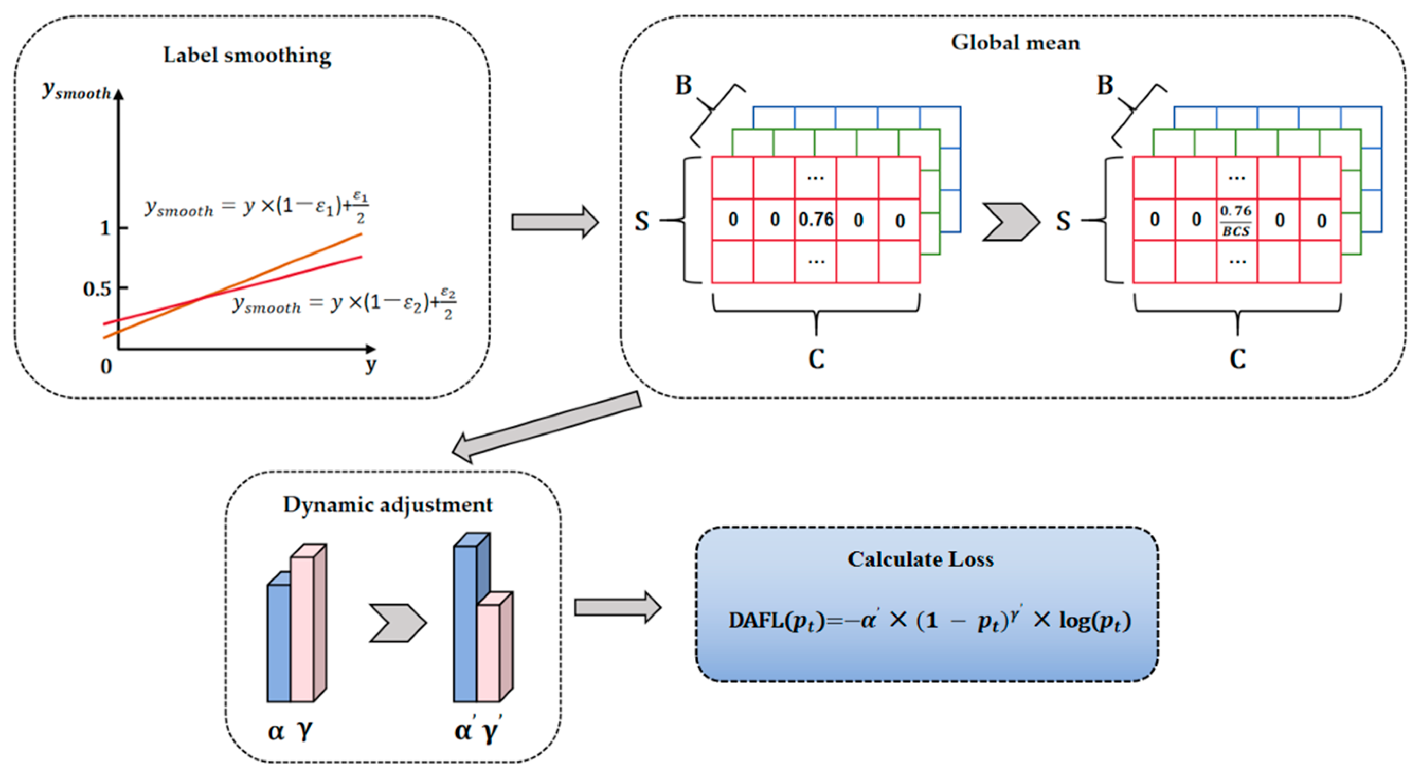
3.4. Dynamic Adaptive Focal Loss

In instance segmentation models, Focal Loss [32] is commonly used as the classification loss. Focal Loss is a loss function designed to improve the performance of classification models when dealing with highly imbalanced datasets. The formula for Focal Loss is as follows:

$$FL\left(p_t\right)=-{\alpha }_t\ast {\left(1-p_t\right)}^{{\gamma }_t}\ast log\left(p_t\right)$$

(17)

Here, $p_t$ is the predicted probability for the true class, ${\alpha }_t$ is a weighting factor that balances the impact of positive and negative samples, and ${\gamma }_t$ is a tuning factor that controls the weight assigned to hard-to-classify samples.

Although Focal Loss can enhance classification accuracy in situations with class imbalance, it presents certain challenges in practical applications. Focal Loss uses fixed ${\alpha }_t$ and ${\gamma }_t$ coefficients during training. Even though these parameters may be optimized prior to training, they remain unchanged throughout the entire process. As a result, Focal Loss is unable to dynamically adjust its parameters in response to varying sample distributions in each training batch. This static parameter configuration may lead to insufficient focus on hard-to-classify samples in some batches or excessive emphasis on easy-to-classify samples, thereby limiting the model’s ability to handle data imbalance effectively.

In underwater environments, the presence of large schools of fish often gathering around coral reefs results in a much higher number of images of marine life compared to other categories. This data imbalance causes the model to be biased towards frequently appearing categories during training while neglecting fewer common objects, thereby affecting the overall performance of the segmentation algorithm. To address this issue, we propose the Dynamic Adaptive Focal Loss (DAFL) method. DAFL introduces label smoothing and dynamically adjusts the ${\alpha }_t$ and ${\gamma }_t$ parameters, enabling the model to adaptively adjust its focus on hard-to-classify samples across different training batches. This dynamic adjustment mechanism not only further mitigates the impact of class imbalance on model performance but also improves segmentation accuracy on extremely imbalanced datasets. The label smoothing is applied to the true label y, defined as

$$y_{smooth}=y\times \left(1-ϵ\right)+{\displaystyle \frac{ϵ}{2}}$$

(18)

where $y$ is the true label, taking values of 0 or 1, indicating whether the sample belongs to a given class. $ϵ$ is the smoothing coefficient. The purpose of label smoothing is to prevent the model from becoming overly confident in the training data, thereby improving generalization.

Next, based on the smoothed label $y_{smooth}$, we calculate the global mean of the labels, denoted as $y_{smooth}$. The smoothed label $y_{smooth}$ is a three-dimensional tensor, consisting of batch size, number of samples, and number of classes. To compute the mean, these dimensions are flattened into a one-dimensional vector, where the total number n is the product of these three dimensions:

$$n=B\times S\times C$$

(19)

where $B$ is the batch size, $S$ is the number of samples, and $C$ is the number of classes. Then, the global mean of the smoothed labels is calculated:

$$y_{smooth}={\displaystyle \frac{1}{n}}\sum _{i=1}^n{y}_{smooth,i}$$

(20)

This mean reflects the class distribution in the current training batch, helping to capture the balance between all classes and mitigate the impact of class imbalance. It also provides insights into the ratio of positive and negative samples and the difficulty of classification. Subsequently, we dynamically adjust the parameter $\alpha$ as follows:

$${\alpha }_t^{\prime }={\alpha }_{initial}\times {\overline{y}}_{smooth}+(1-{\overline{y}}_{smooth})\times (1-{\alpha }_{initial})$$

(21)

In this equation, ${\overline{y}}_{smooth}$ represents the proportion of positive samples. When the proportion of positive samples is high, the value of ${\alpha }_t^{\prime }$ increases, approaching ${\alpha }_{initial}$, giving lower weight to the positive samples and reducing the penalty on easy samples. When the proportion of positive samples is low, ${\alpha }_t^{\prime }$ decreases, approaching $1-{\alpha }_{initial}$, assigning higher weight to the positive samples and increasing the focus on difficult samples. This dynamic adjustment effectively balances the weights between positive and negative samples, allowing the model to learn effectively even in the presence of class imbalance. The formula for dynamically adjusting the parameter $\gamma$ is

$${\gamma }_t^{\prime }={\gamma }_{initial}\times (1-{\overline{y}}_{smooth})$$

(22)

This equation adjusts ${\gamma }_t^{\prime }$ based on the change in the proportion of positive samples ${\overline{y}}_{smooth}$ When the proportion of positive samples is low, indicating that there are more difficult-to-classify samples in the current batch, the value of ${\gamma }_t^{\prime }$ increases, approaching ${\gamma }_{initial}$, which gives higher weight to these difficult samples. When the proportion of positive samples is high, ${\gamma }_t^{\prime }$ decreases, approaching zero, thus reducing the penalty on easy-to-classify samples. Through this dynamic adjustment, the modified Focal Loss can adaptively increase the loss weight for difficult samples in class-imbalanced situations, significantly improving the model’s classification performance. The dynamic Focal Loss calculation is designed as follows:

$${DAFL\left(p_t\right)=-\alpha }_t^{\prime }\times {\left(1-p_t\right)}^{{\gamma }_t^{\prime }}\times \mathrm{l}\mathrm{o}\mathrm{g}(p_t)$$

(23)

Finally, the overall loss function for the AASNet network is divided into three parts and can be expressed as

$$L_{total}={\lambda }_{cls}\ast L_{cls}+{\lambda }_{box}\ast L_{box}+{\lambda }_{mask}\ast L_{mask}$$

(24)

where ${\lambda }_{cls}$, ${\lambda }_{box}$, and ${\lambda }_{mask}$ are the weighting factors for the classification, bounding box regression, and segmentation losses, respectively. In our experiments, we assign a weight of 0.5 to the ${\lambda }_{cls}$, 7.5 to the ${\lambda }_{box}$, and 0.2 to the ${\lambda }_{mask}$.

To address the extreme imbalance in underwater instance segmentation datasets, the classification loss $L_{cls}$ uses our proposed Dynamic Adaptive Focal Loss (DAFL); the Dynamic Adaptive Focal Loss schematic illustration diagram is shown in Figure 4. For the bounding box regression loss $L_{box}$, we adopt the CIoU loss [33] and Distribution Focal Loss [34] to enhance the prediction accuracy and alignment between the predicted and ground truth boxes. The segmentation loss $L_{mask}$ employs binary cross-entropy loss to measure the difference between the predicted and ground truth masks. These two loss functions are designed to be consistent with the original YOLOv9 approach.

4. Results and Discussion

4.1. Dataset Sources

(1)

UIIS dataset: This is the first general underwater image instance segmentation dataset, released in 2023. This dataset includes seven challenging categories, such as fish, divers, reefs, and more. The UIIS dataset consists of 4628 images, divided into training, validation, and test sets with a ratio of 7.4:1.3:1.3. The images in the dataset vary in resolution, including $240\times 320$ pixel images captured by low-resolution handheld cameras, and $720\times 1280$ pixel images taken by medium- to high-resolution industrial equipment, ensuring diversity and high quality in the dataset. Among the images, fish constitute a significant proportion. For instance, there are 16,749 fish instances annotated in images. These annotations are valuable for fish detection and behavioral analysis in smart fish farming.

(2)

USIS10K dataset: This is the first large-scale underwater salient instance segmentation dataset, released in 2024. This dataset contains 10,632 images with pixel-level annotations from various underwater scenes and is divided into training, validation, and test sets with a ratio of 7:1.5:1.5. The dataset includes two types of annotations: single-class annotations, where all labels are marked as foreground, and detailed annotations, with seven sub-categories such as fish, ruins, aquatic plants, etc. In the USIS10K dataset, there are 9663 fish instances annotated. This detailed annotation provides high-quality training resources for tasks such as fish identification, disease detection, and water quality monitoring in smart fish farming. The diversity of fish annotations in the dataset supports both single-category and multi-category segmentation tasks, enhancing the model’s adaptability in complex underwater environments.

4.2. Evaluation Metric and Details

The standard mask AP metric is employed as the evaluation criterion, comprehensively assessing the model’s performance through mAP, AP50, AP75, and a range of different IoU thresholds. In addition to the newly designed components, all backbone and method hyperparameters remain consistent with the original YOLOv9 approach. In the Dynamic Adaptive Focal Loss, we set the smoothing coefficient ϵ to 0.1, initial alpha to 0.25, and initial gamma to 1.5. These parameters are determined through a series of experiments to optimize performance for the current task. The model is trained with a batch size of 12 per GPU using the SGD optimizer, with an initial learning rate of $1\times {10}^{-2}$. AASNet is implemented in PyTorch 1.7.1, and all experiments are conducted on an NVIDIA P40 GPU. Each training cycle consists of 300 epochs.

To evaluate segmentation performance, we utilize mAP (mean Average Precision) as the primary evaluation metric. mAP represents the average segmentation performance across multiple classes and is defined as

$$mAP={\displaystyle \frac{\sum _{i=1}^{N}A{P}_i}{N}}$$

(25)

where $N$ is the number of classes. The Average Precision (AP) for each class is calculated by integrating the precision–recall (PR) curve:

$$AP={\int }_0^{1}p\left(r\right)dr$$

(26)

Here, $p\left(r\right)$ represents the precision at a given recall value, used to evaluate the prediction accuracy of the model, and is defined as

$$Precision={\displaystyle \frac{TP}{TP+FP}}$$

(27)

where $TP$ represents true positive samples, and $FP$ represents false positive samples. Additionally, recall is another important metric that indicates the proportion of actual positive samples correctly identified by the model, and is defined as

$$Recall={\displaystyle \frac{TP}{FN+TP}}$$

(28)

Here, $FN$ represents false negative samples. In addition, we use AP50 and AP75 to further evaluate the model’s performance under different IoU (Intersection over Union) thresholds. AP50 measures the Average Precision at an IoU threshold of 0.5, indicating the model’s performance under more lenient criteria, while AP75 represents the average precision at an IoU threshold of 0.75, used for stricter evaluation. Together, these metrics provide a comprehensive assessment of the model’s segmentation performance.

4.3. Comparative Experimental Results

(1)

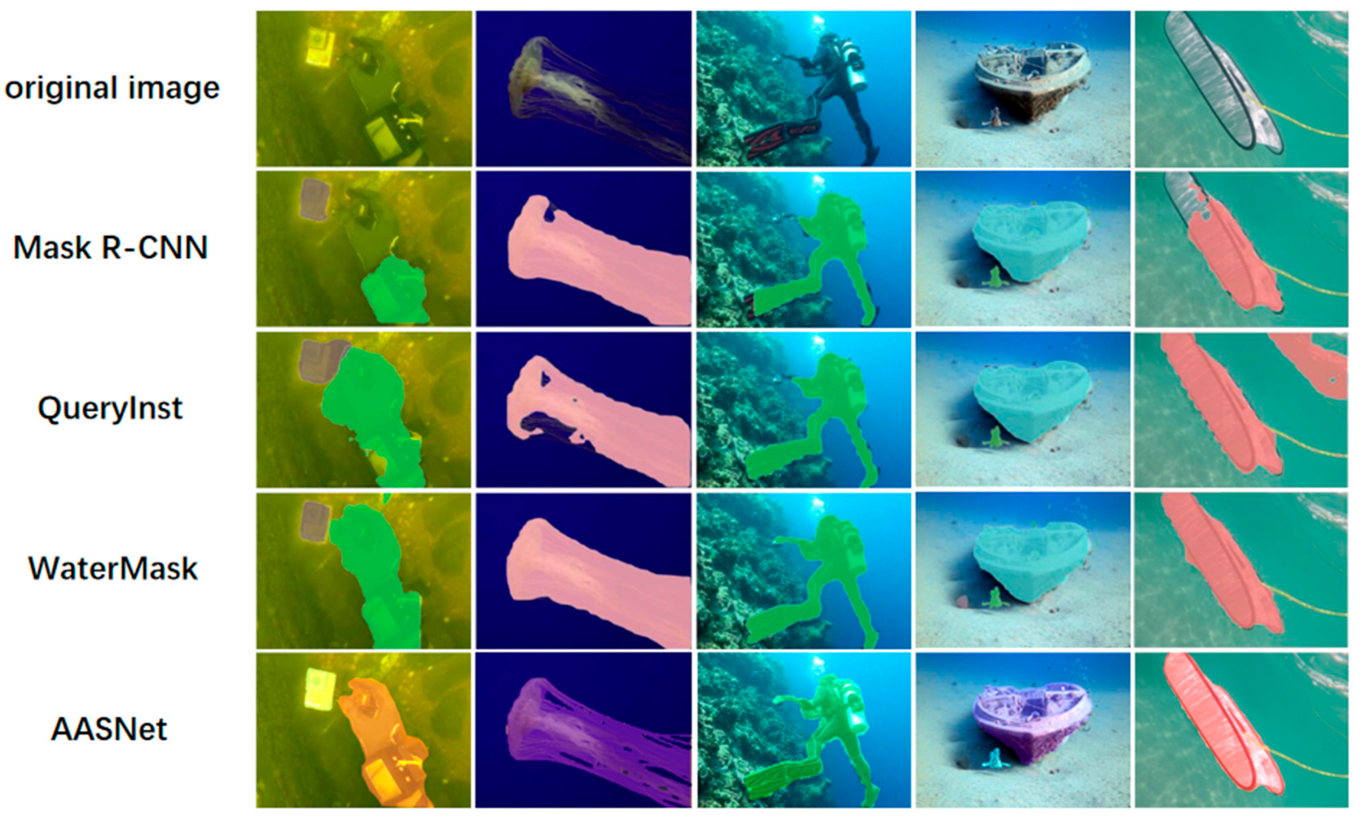
Performance on UIIS: We present the results of our method on the UIIS underwater image instance segmentation dataset and compare them with other popular instance segmentation methods. As shown in

Table 1. Comparison of instance segmentation methods on the UIIS Dataset. Quantitative results demonstrate that our AASNet model achieves the best segmentation performance. The bold font indicates the best effect.

Methods	Backbone	mAP	AP50	AP75
Mask RCNN [5]	ResNet-101	23.4	40.9	25.3
Mask Scoring R-CNN [35]	ResNet-101	24.6	41.9	26.5
Cascade Mask R-CNN [36]	ResNet-101	25.5	42.8	27.8
BMask R-CNN [12]	ResNet-101	22.1	36.2	24.4
Point Rend [11]	ResNet-101	25.9	43.4	27.6
SOLOv2 [37]	ResNet-101	24.5	40.9	25.1
QueryInst [38]	ResNet-101	26.0	42.8	27.3
Mask2Former [39]	ResNet-101	25.7	38.0	27.7
RDPNet [40]	ResNet-101	20.6	38.7	19.4
Mask Transfiner [41]	ResNet-101	24.6	42.1	26.0
WaterMask [8]	ResNet-101	27.2	43.7	29.3
USIS-SAM [10]	ViT-H	29.4	45.0	32.3
AASNet	GELAN+LCA	31.7	49.5	35.1

, our proposed method achieves a new state-of-the-art on UIIS with an mAP score of 31.7, surpassing USIS-SAM by 2.3 points. In terms of AP50 and AP75, our method exceeds USIS-SAM by 4.5 points and 2.8 points, respectively. This indicates that our approach provides better underwater instance segmentation with higher localization accuracy. Additionally, the AASNet model has a parameter count of 27.84 M, demonstrating exceptional performance in real-time underwater instance segmentation tasks. We conduct tests on an NVIDIA P40 GPU with a batch size of 12, where the model achieves an inference time of only 28.9 milliseconds when processing 640 × 640 resolution images. In comparison, the WaterMask [8] model has a parameter count of 66.55 M, with an inference time of 180.5 milliseconds under the same configuration. Clearly, AASNet offers significant advantages in computational efficiency.

Figure 5 presents a visual comparison of our method with existing techniques on the UIIS dataset. It can be observed that our method excels in segmenting the overall shape of prominent instances, even in challenging regions. For example, in the second column of the figure, our method accurately segments the gaps between the tentacles of a jellyfish. Additionally, our model performs exceptionally well in predicting boundaries and details, as shown in the third and fifth columns of the figure, where the boundaries of the diver and the plankton net predicted by our model are much closer to the ground truth masks.

As shown in Figure 6, the training and validation loss curves on the UIIS dataset reveal the model’s performance during training. The training loss steadily decreases throughout the epochs, indicating that the model effectively learns and minimizes error on the training data. Meanwhile, the validation loss remains relatively stable, with only slight fluctuations, suggesting that the model is able to generalize well to unseen data without significant overfitting. Regarding the model’s instance segmentation performance, the steady decline in training loss and stable validation loss reflect a robust ability to segment instances accurately. The model shows consistent improvements in both the training and validation phases, which indicates strong performance in segmenting objects within the UIIS dataset.

The analysis of the confusion matrix in Figure 7 shows that the model performs excellently in handling the “diver” and “fish” categories, with high accuracy and minimal confusion. However, for the “aquatic plants” and “robots” categories, the model exhibits some misclassification, particularly with confusion between the “background” class and other targets. Overall, the model effectively distinguishes most categories, but further optimization is needed, especially for categories affected by background interference in complex underwater environments.

(2)

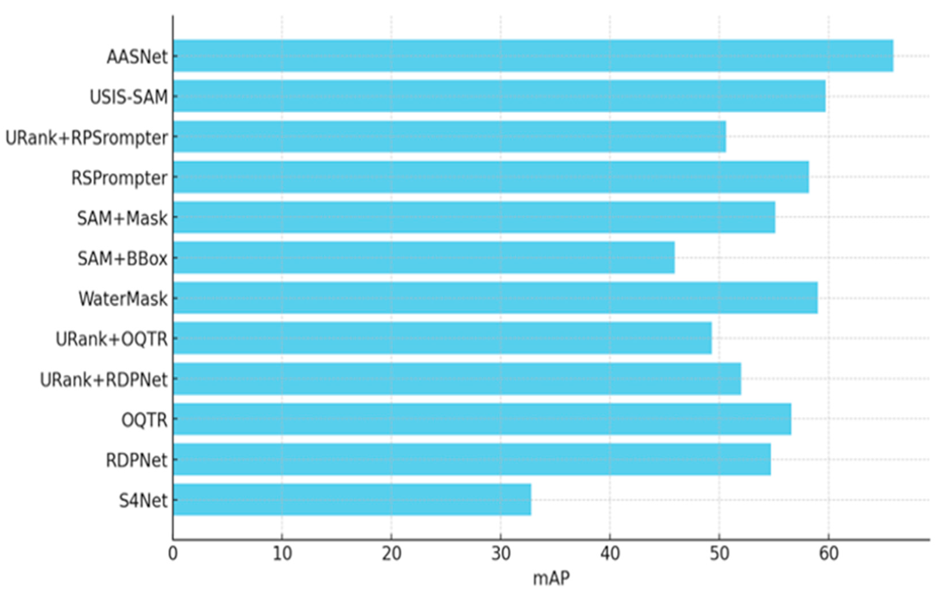
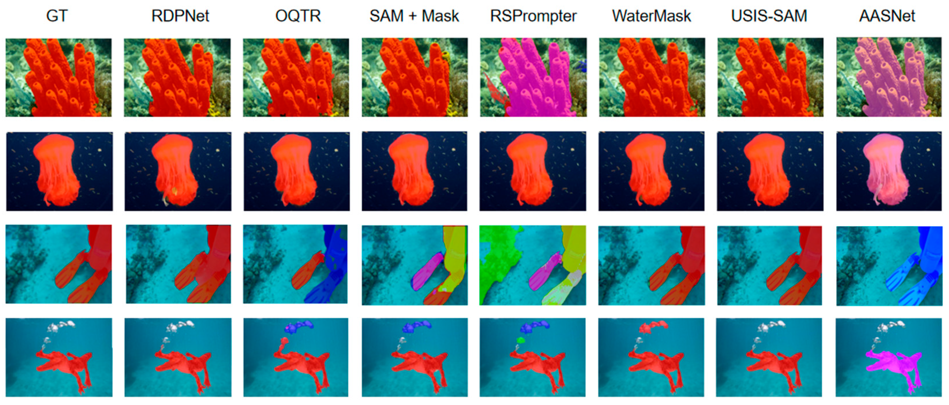
Performance on USIS10K:

Table 2. Comparison of instance segmentation methods on the USIS10K Dataset. Bold values indicate the best performance in each column. The bold font indicates the best effect.

Method	Backbone	Class-Agnostic			Multi-Class
		mAP	AP50	AP75	mAP	AP50	AP75
S4Net [42]	ResNet-50	32.8	64.1	27.3	23.9	43.5	24.4
RDPNet [40]	ResNet-50	53.8	77.8	61.9	37.9	55.3	42.7
RDPNet [40]	ResNet-101	54.7	78.3	63.0	39.3	55.9	45.4
OQTR [43]	ResNet-50	56.6	79.3	62.6	19.7	30.6	21.9
URank+RDPNet [40]	ResNet-101	52.0	77.0	62.0	35.9	52.5	41.4
URank+OQTR [43]	ResNet-50	49.3	74.3	56.2	32.1	44.1	23.3
WaterMask [8]	ResNet-50	58.3	80.2	66.5	37.7	54.0	42.5
WaterMask [8]	ResNet-101	59.0	80.6	67.2	38.7	54.9	43.2
SAM+BBox [44]	ViT-H	45.9	65.9	52.1	26.4	38.9	29.0
SAM+Mask [44]	ViT-H	55.1	80.2	60.9	38.5	55.4	44.8
RSPrompter [45]	ViT-H	58.2	79.9	65.9	38.0	55.0	44.6
URank+RPSrompter [45]	ViT-H	50.6	74.4	56.6	38.5	55.0	43.3
USIS-SAM [10]	ViT-H	59.7	81.6	67.7	43.1	59.0	48.5
AASNet	GELAN+LCA	65.9	86.0	73.1	47.4	62.1	52.2

shows the performance comparison with state-of-the-art methods. The results of the histogram visualization of the average accuracy of each advanced method are shown in Figure 8. The experimental results demonstrate that our model performs better when the data volume is expanded. Our method achieves an mAP that is 4.6 points higher than USIS-SAM under multi-label annotations and 6.2 points higher under single-label annotations. In both annotation settings, AP50 and AP75 also reach optimal values, further proving the effectiveness of our approach.

The visualization results on the USIS10K dataset, shown in Figure 9, demonstrate the model’s outstanding performance in handling complex underwater scenes. Despite the presence of background complexity, color deviation, and the effects of light scattering and absorption in underwater images, the model accurately identifies and segments multiple instances, achieving clear separation between foreground and background. Notably, even when the ground truth labels do not fully annotate all instances, the model successfully predicts unannotated fish. This is attributed to the Linear Correlation Attention (LCA) mechanism, which effectively captures linear correlations between features, enabling consistent handling of color variations caused by lighting changes and ensuring semantic consistency. The LCA module enhances the model’s understanding of target objects in complex environments, allowing it to accurately identify the contours and details of objects even under significant lighting variations, thereby significantly improving segmentation performance.

Figure 10 presents a visual comparison of our method with existing techniques on the USIS10K dataset. The results indicate that Dynamic Adaptive Focal Loss (DAFL) significantly enhances the ability to handle class-imbalanced data. Unlike some advanced methods that incorrectly classify divers and bubbles, our approach accurately classifies and effectively segments instances.

The loss curves on the USIS10K dataset are shown in Figure 11, revealing that the model learns effectively across all tasks, as evidenced by the steady decrease in training losses for box, segmentation, and classification over epochs. This indicates that the model is successfully minimizing errors and improving its performance during training. The validation losses for these components also stabilize after a few epochs, suggesting that the model generalizes well to unseen data. The small gap between training and validation losses indicates minimal overfitting and strong generalization ability. Overall, the model demonstrates good performance on the USIS10K dataset, with effective optimization and minimal overfitting.

The analysis of the confusion matrix in Figure 12 shows that the model performs well in distinguishing categories such as “wrecks/ruins” and “human divers”, with high accuracy and minimal confusion between these categories. However, there are misclassifications for the “background” category, which is often confused with other classes, particularly “wrecks/ruins”, “fish”, and “sea-floor”. Additionally, some misclassification occurs between “fish” and “reefs”. While the model is effective at differentiating most categories, further improvements are needed for categories prone to confusion, such as “background” and “sea-floor”, especially in more complex environments.

Notably, the model’s performance on the “fish” category is better in the USIS10K dataset, with an accuracy of 86%, compared to 60% in the UIIS dataset, demonstrating an overall improvement in the model’s classification capabilities on the USIS10K dataset.

4.4. Ablation Results and Analysis

To verify the effectiveness of different components of the proposed method, we conduct several ablation experiments on the UIIS dataset to demonstrate performance.

(1)

Overall Ablation Study: To analyze the importance of each proposed component, we report the overall ablation study in

Table 3. Impact results of different modules in proposed AASNet, the ✓ denotes the use of this method.

LCA	DAFL	mAP	AP50	AP75
		28.5	45.9	31.2
✓		30.9	48.4	34.3
✓	✓	31.7	49.5	35.1

. We gradually add the LCA module and Dynamic Adaptive Focal Loss to the YOLOv9 baseline. The results show that the LCA module improves the mAP by 2.4, demonstrating that the LCA module effectively enhances the model’s ability to handle lighting variations and color differences in complex underwater environments, optimizing the consistency of semantic information and thereby improving instance segmentation accuracy. Additionally, Dynamic Adaptive Focal Loss further increases the mAP to 31.7, with simultaneous improvements in the other two metrics, proving that this loss function performs better in classification, thus enhancing overall segmentation accuracy.

(2)

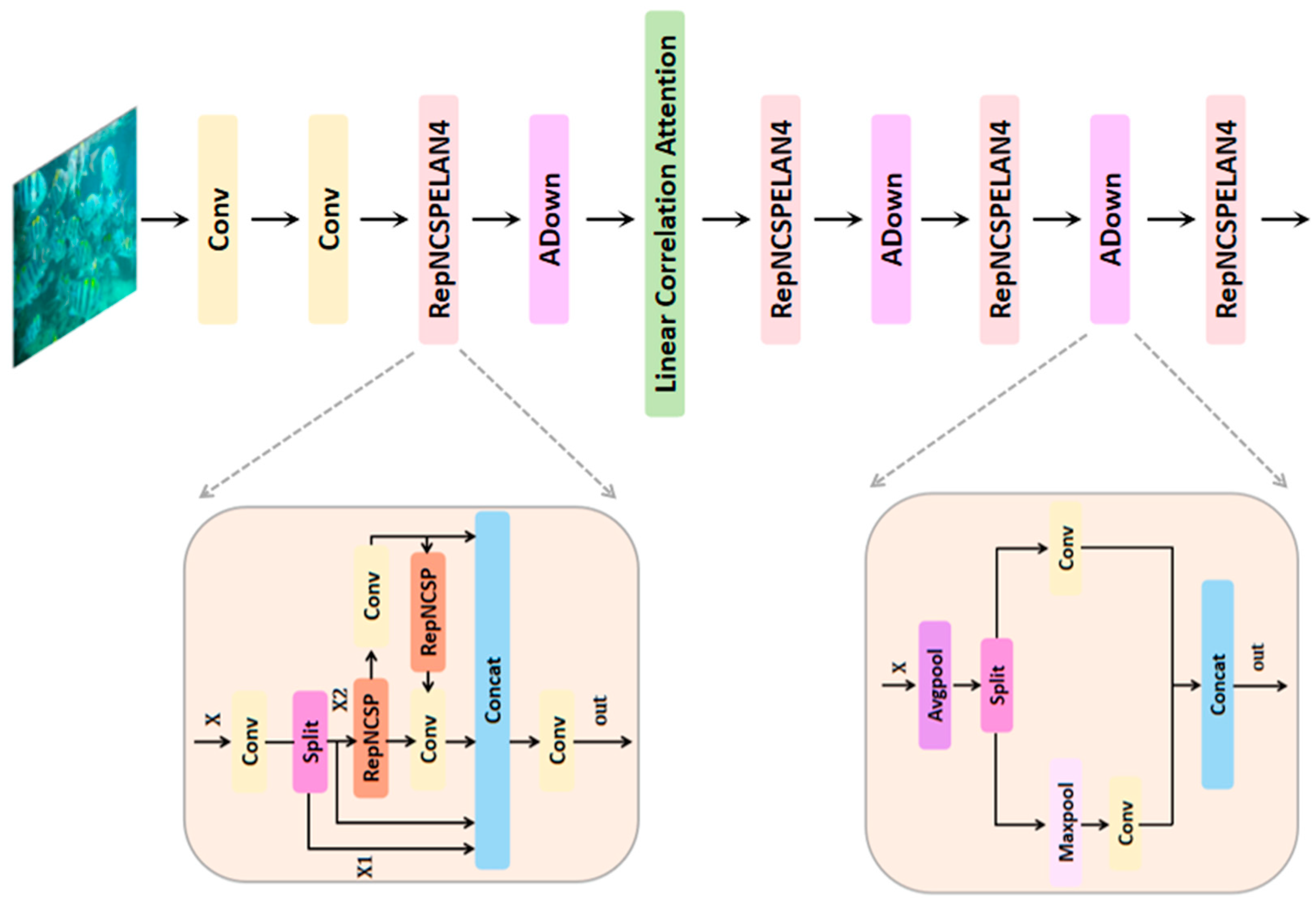
Ablation study on Linear Correlation Attention Module: We conduct ablation experiments to evaluate the placement of the LCA module at different levels of the backbone, testing it at None, P1, P2, P3, P4, and P5. As shown in

Table 4. Position comparison results. Compared to other positions, the P4 layer effectively captures advanced abstract features while maintaining sufficient spatial resolution, enabling the LCA module to more effectively handle lighting variations in underwater instance segmentation. The bold font indicates the best effect.

Position	mAP	AP50	AP75
None	28.5	45.9	31.2
P1	29.5	48.2	32.2
P2	29.6	46.1	32.5
P3	30.6	47.7	33.8
P4	30.9	48.4	34.3
P5	30.5	47.6	33.6

, placing the module at the P4 layer yields the best results, with mAP increasing by 2.4 to 30.9 and AP50 and AP75 reaching 48.4 and 34.3, respectively. This is because the P4 layer achieves an ideal balance between spatial resolution and semantic information in the feature map. In shallower layers (such as P1 and P2), although the spatial resolution is high, most captured features are low-level, making it difficult to support precise segmentation in complex underwater scenes. In deeper layers (such as P5), while higher-level abstract features are captured, the significant reduction in spatial resolution results in insufficient precision in local feature extraction. The P4 layer occupies a critical intermediate position, effectively capturing advanced levels of abstract features while maintaining sufficient spatial resolution. Therefore, adding the LCA module at the P4 layer enhances the model’s ability to capture semantic features in complex underwater environments. It preserves essential detail and improves segmentation performance, leading to better results when addressing lighting variations, color differences, and complex backgrounds.

(3)

Ablation study on Dynamic Adaptive Focal Loss: To analyze the effectiveness of Dynamic Adaptive Focal Loss (DAFL), we present the ablation study on the loss function in

Table 5. Ablation study of DAFL on loss functions. The results show that the introduction of label smoothing and global mean achieves the best performance, with a mAP improvement of 0.8 points, the ✓ denotes the use of this method.

Label Smoothing	Global Mean	mAP	AP50	AP75
		30.9	48.4	34.3
✓		31.2	48.7	34.6
	✓	31.4	49.2	35.2

. The results show that introducing label smoothing into Focal Loss improves mAP by 0.3. This suggests that label smoothing enhances the model’s generalization ability, especially for hard-to-classify samples, by reducing overfitting. Additionally, incorporating a dynamic calculation strategy based on the global mean into Focal Loss improves mAP by an additional 0.5. This demonstrates that the method automatically adjusts the model’s focus on hard and easy samples, depending on the class distribution within the current training batch, thereby improving classification accuracy. When both methods are applied together, the model achieves optimal performance. Overall, Dynamic Adaptive Focal Loss significantly boosts the model’s classification ability and robustness, particularly in handling highly imbalanced instance segmentation tasks.

4.5. Extended Experiments and Analysis

In fact, the proposed AASNet model can not only play a good role in smart fishery applications but can also be transferred to other smart agriculture applications in non-underwater environments, which can well solve various tasks of image detection and segmentation. For further verification, our AASNet is again applied to the custom-built SDD dataset of intelligent agriculture, which is collected through the agricultural Internet of Things and camera equipment to monitor the growth status of strawberries and symptoms of leaf pests and diseases. The experimental results and visualizations for this additional dataset are provided below, demonstrating the migration generalization ability and application potential of the proposed AASNet across different scenarios.

Table 6. Segmentation results on SDD dataset (APm: mAP of mask; APb: mAP of bbox).

Methods	Backbone	APm	APb
Mask R-CNN	Resnet50	51.6	52.8
TensorMask	Resnet50	50.7	52.9
CenterMask	Resnet50	53.4	56.7
BlendMask	Resnet50	55.3	57.3
MS R-CNN	Resnet50	52.3	52.9
Bmask R-CNN	Resnet50	53.4	55.8
Cascade Mask	Swint	52.4	53.0
AASNet (ours)	GELAN+LCA	59.1	62.2

presents the detection and segmentation performance of several segmentation models on a crop disease detection dataset. When using the GELAN+LCA backbone network, our proposed method achieves suboptimal Average Precision (APm) performance of 59.1% and 80.5% on two datasets, respectively. On the SDD dataset, it outperforms Mask R-CNN, TensorMask, CenterMask, BlendMask, MS R-CNN, Bmask R-CNN, and Cascade Mask by 7.5%, 8.4%, 5.7%, 3.8%, 6.8%, 5.7%, and 6.7%, respectively. On the PVDS dataset, it outperforms Mask R-CNN, TensorMask, CenterMask, BlendMask, MS R-CNN, Bmask R-CNN, and Cascade Mask by 10.2%, 10.7%, 6.1%, 5.7%, 9.2%, 7.4%, and 6.3%, respectively. These results demonstrate that our model can adapt to different application scenarios, achieving optimal disease segmentation results.

Figure 13 presents the instance segmentation results of the SDD dataset across six different scenes. Regardless of whether the target contours are regular or irregular, our model consistently delivers precise segmentation and accurate class recognition, particularly in scenarios with simple backgrounds. Even in complex scenes with shadows, as shown in Figure 13I,III–V, our model maintains the ability to accurately distinguish targets, demonstrating robust performance. Overall, our model exhibits exceptional performance in practical detection tasks, with more accurate segmentation results, a lower risk of missed detections, and the ability to consistently maintain high-quality segmentation in various environmental conditions. These advantages highlight the significant application value of our model in crop disease detection within agricultural environments, validating its effectiveness in real-world scenarios.

5. Conclusions

In smart fishery aquaculture, traditional practices face challenges, such as resource constraints and environmental pollution, as the demand for aquatic products increases. While smart fisheries enhance aquaculture efficiency through advanced technologies, underwater image segmentation still encounters difficulties due to variations in water quality, lighting, and data imbalance. As a result, underwater fish image segmentation has become a key technology for improving aquaculture efficiency, monitoring water quality, and increasing production. It enables accurate identification of fish locations and behaviors, aiding in underwater environment monitoring, fish health assessment, and disease warning.

To address these challenges, this paper presents a new underwater instance segmentation model. AASNet introduces the Linear Correlation Attention (LCA) mechanism, which captures linear correlations between features to effectively handle color inconsistencies in underwater images, thereby improving segmentation accuracy. Additionally, the proposed Dynamic Adaptive Focus Loss (DAFL) dynamically adjusts the model’s attention to difficult-to-classify samples, addressing the data imbalance issue and enhancing classification performance. Experiments on the UIIS and USIS10K datasets demonstrate that AASNet outperforms existing methods in both accuracy and inference speed. Specifically, AASNet achieves a mean Average Precision (mAP) of 31.7 on the UIIS dataset, surpassing USIS-SAM by 2.3 points, and a mAP 4.6 points higher on the USIS10K dataset. Moreover, AASNet’s inference time of 28.9 ms is significantly faster than the 180.5 ms of the WaterMask model. These results indicate that AASNet effectively addresses lighting changes and background interference in complex underwater environments, improving both segmentation accuracy and efficiency.

Despite its success, AASNet still faces some challenges. Future research will focus on optimizing the model’s real-time processing capabilities, improving segmentation performance for rare objects, enhancing its adaptability to extreme conditions, and exploring integration with water quality monitoring and automated feeding systems for more comprehensive intelligent aquaculture management [46,47].

References

1. Qin, Q.Y.; Liu, J.Y.; Chen, Y.H.; Wang, X.R.; Chu, T.J. Knowledge Map of the Development Trend of Smart Fisheries in China: A Bibliometric Analysis. Fishes 2024, 9, 258. [Google Scholar] [CrossRef]
2. Li, P.; Han, H.; Zhang, S.; Fang, H.; Fan, W.; Zhao, F.; Xu, C. Reviews on the development of digital intelligent fisheries technology in aquaculture. Aquac. Int. 2025, 33, 191. [Google Scholar]
3. Wu, Z.; Xiong, M.; Cheng, T.; Dai, Y.; Zhang, S.; Fan, W.; Cui, X. Application Prospects and Challenges of VHF Data Exchange System (VDES) in Smart Fisheries. J. Mar. Sci. Eng. 2025, 13, 250. [Google Scholar] [CrossRef]
4. Hafiz, A.M.; Bhat, G.M. A survey on instance segmentation: State of the art. Int. J. Multimed. Inf. Retr. 2020, 9, 171–189. [Google Scholar] [CrossRef]
5. He, K.; Gkioxari, G.; Dollar, P.; Girshick, R. Mask r-cnn. In Proceedings of the IEEE International Conference on Computer Vision, Venice, Italy, 22–29 October 2017; pp. 2961–2969. [Google Scholar]
6. Zhang, T.; Wei, S.; Ji, S. E2ec: An end-to-end contourbased method for high-quality high-speed instance segmentation. In Proceedings of the IEEE Conference on Computer Vision and Pattern Recognition, New Orleans, LA, USA, 18–24 June 2022; pp. 4443–4452. [Google Scholar]
7. Jian, M.; Liu, X.; Luo, H.; Lu, X.; Yu, H.; Dong, J. Underwater image processing and analysis: A review. Signal Process. Image Commun. 2021, 91, 116088. [Google Scholar] [CrossRef]
8. Lian, S.; Li, H.; Cong, R.; Li, S.; Zhang, W.; Kwong, S. Watermask: Instance segmentation for underwater imagery. In Proceedings of the IEEE International Conference on Computer Vision, Paris, France, 2–3 October 2023; pp. 1305–1315. [Google Scholar]
9. Kong, J.; Wang, H.; Yang, C.; Jin, X.; Zuo, M.; Zhang, X. A spatial feature-enhanced attention neural network with high-order pooling representation for application in pest and disease recognition. Agriculture 2022, 12, 500. [Google Scholar] [CrossRef]
10. Lian, S.; Li, C.; Liu, Z.; Zhang, X.; Yang, L.; Wang, Z.; Li, J. Diving into Underwater: Segment Anything Model Guided Underwater Salient Instance Segmentation and A Large-scale Dataset. In Proceedings of the 41st International Conference on Machine Learning, Vienna, Austria, 21–27 July 2024; pp. 29545–29559. [Google Scholar]
11. Kirillov, A.; Wu, Y.; He, K.; Girshick, R. PointRend: Image Segmentation as Rendering. In Proceedings of the IEEE/CVF Conference on Computer Vision and Pattern Recognition, Seattle, WA, USA, 14–19 June 2020; pp. 9799–9808. [Google Scholar]
12. Cheng, B.; Wei, Y.; Shi, H.; Feris, R.S.; Xiong, J.; Huang, T.S. Boundary-preserving Mask R-CNN. In Proceedings of the European Conference on Computer Vision, Glasgow, UK, 23–28 August 2020; pp. 660–676. [Google Scholar]
13. Zhang, Y.; Wu, J.; Li, S.; Liu, H. Self-Balanced R-CNN for Instance Segmentation. J. Vis. Commun. Image Represent. 2022, 82, 103449. [Google Scholar]
14. Kong, J.L.; Wang, H.X.; Wang, X.Y.; Jin, X.B.; Fang, X.; Lin, S. Multi-stream hybrid architecture based on cross-level fusion strategy for fine-grained crop species recognition in precision agriculture. Comput. Electron. Agric. 2021, 185, 106134. [Google Scholar] [CrossRef]
15. Kirillov, A.; Levinkov, E.; Andres, B.; Savchynskyy, B.; Schiele, B. InstanceCut: From Edges to Instances with MultiCut. In Proceedings of the IEEE Conference on Computer Vision and Pattern Recognition, Honolulu, HI, USA, 21–26 July 2017; pp. 5008–5017. [Google Scholar]
16. Liu, S.; Jia, J.; Fidler, S.; Urtasun, R. SGN: Sequential Grouping Networks for Instance Segmentation. In Proceedings of the IEEE International Conference on Computer Vision, Venice, Italy, 22–29 October 2017; pp. 3496–3504. [Google Scholar]
17. Bai, M.; Urtasun, R. Deep Watershed Transform for Instance Segmentation. In Proceedings of the IEEE Conference on Computer Vision and Pattern Recognition, Honolulu, HI, USA, 21–26 July 2017; pp. 5221–5229. [Google Scholar]
18. Wang, C.Y.; Yeh, I.H.; Liao, H.Y.M. Yolov9: Learning what you want to learn using programmable gradient information. arXiv 2024, arXiv:2402.13616. [Google Scholar]
19. Islam, M.J.; Xia, Y.; Sattar, J. Fast underwater image enhancement for improved visual perception. IEEE Robot. Autom. Lett. 2020, 5, 3227–3234. [Google Scholar] [CrossRef]
20. Zhuang, P.; Wang, Y.; Qiao, Y. Wildfish: A large benchmark for fish recognition in the wild. In Proceedings of the the 26th ACM International Conference on Multimedia, San José, Costa Rica, 22–26 October 2018; pp. 1301–1309. [Google Scholar]
21. Islam, M.J.; Edge, C.; Xiao, Y.; Luo, P.; Mehtaz, M.; Morse, C.; Enan, S.S.; Sattar, J. Semantic segmentation of underwater imagery: Dataset and benchmark. In Proceedings of the IEEE/RSJ International Conference on Intelligent Robots and Systems, Las Vegas, Nevada, USA, 25–29 October 2020; pp. 1769–1776. [Google Scholar]
22. Garcia-D’Urso, N.E.; Galan-Cuenca, A.; Climent-Perez, P.; Saval-Calvo, M.; Azorin-Lopez, J.; Fuster-Guillo, A. Efficient instance segmentation using deep learning for species identification in fish markets. In Proceedings of the International Joint Conference on Neural Networks, Padua, Italy, 18–23 July 2022; pp. 1–8. [Google Scholar]
23. Imada, A.; Katayama, T.; Song, T.; Shimamoto, T. YOLOX based underwater object detection for inshore aquaculture. In Proceedings of the OCEANS 2022, Hampton Roads, VI, USA, 17–20 October 2022; IEEE: New York, NY, USA, 2022; pp. 1–5. [Google Scholar]
24. Li, D.; Yang, Y.; Zhao, S.; Ding, J. Segmentation of underwater fish in complex aquaculture environments using enhanced Soft Attention Mechanism. Environ. Model. Softw. 2024, 181, 106170. [Google Scholar]
25. Zheng, Y.Y.; Kong, J.L.; Jin, X.B.; Wang, X.Y.; Zuo, M. CropDeep: The crop vision dataset for deep-learning-based classification and detection in precision agriculture. Sensors 2019, 19, 1058. [Google Scholar] [CrossRef] [PubMed]
26. Khudoyberdiev, A.; Jaleel, M.A.; Ullah, I.; Kim, D. Enhanced Water Quality Control Based on Predictive Optimization for Smart Fish Farming. Comput. Mater. Contin. 2023, 75, 5471–5499. [Google Scholar]
27. Kaur, G.; Adhikari, N.; Krishnapriya, S.; Wawale, S.G.; Malik, R.Q.; Zamani, A.S.; Perez-Falcon, J.; Osei-Owusu, J. Recent advancements in deep learning frameworks for precision fish farming opportunities, challenges, and applications. J. Food Qual. 2023, 2023, 4399512. [Google Scholar]
28. Kong, J.L.; Fan, X.M.; Jin, X.B.; Lin, S.; Zuo, M. A Variational Bayesian Inference-Based En-Decoder Framework for Traffic Flow Prediction. IEEE Trans. Intell. Transp. Syst. 2023, 25, 2966–2975. [Google Scholar] [CrossRef]
29. Kong, J.; Fan, X.; Zuo, M.; Deveci, M.; Jin, X.; Zhong, K. ADCT-Net: Adaptive traffic forecasting neural network via dual-graphic cross-fused transformer. Inf. Fusion 2023, 103, 102122. [Google Scholar] [CrossRef]
30. Dong, Z.; Kong, J.; Yan, W.; Wang, X.; Li, H. Multivariable High-Dimension Time-Series Prediction in SIoT via Adaptive Dual-Graph-Attention Encoder-Decoder with Global Bayesian Optimization. IEEE Internet Things J. 2024, 11, 32956–32968. [Google Scholar] [CrossRef]
31. Wang, X.; Girshick, R.; Gupta, A.; He, K. Non-Local Neural Networks. In Proceedings of the IEEE Conference on Computer Vision and Pattern Recognition, Salt Lake City, UT, USA, 18–22 June 2018; pp. 7794–7803. [Google Scholar]
32. Lin, T.-Y.; Goyal, P.; Girshick, R.; He, K.; Dollar, P. Focal Loss for Dense Object Detection. In Proceedings of the IEEE International Conference on Computer Vision, Venice, Italy, 22–29 October 2017; pp. 2980–2988. [Google Scholar]
33. Zheng, Z.; Wang, P.; Liu, W.; Li, J.; Ye, R.; Ren, D. Distance-IoU Loss: Faster and Better Learning for Bounding Box Regression. In Proceedings of the AAAI Conference on Artificial Intelligence, New York, NY, USA, 7–12 February 2020; pp. 12993–13000. [Google Scholar]
34. Li, Z.; Wang, W.; Wu, L.; Chen, S.; Hu, X.; Li, J.; Tang, J.; Yang, J. Generalized Focal Loss: Learning Qualified and Distributed Bounding Boxes for Dense Object Detection. Adv. Neural Inf. Process. Syst. 2020, 33, 21002–21012. [Google Scholar]
35. Huang, Z.; Huang, L.; Gong, Y.O.; Huang, C.; Wang, X. Mask scoring r-cnn. In Proceedings of the IEEE Conference on Computer Vision and Pattern Recognition, Long Beach, CA, USA, 15–20 June 2019. [Google Scholar]
36. Cai, Z.; Vasconcelos, N. Cascade r-cnn: Delving into high quality object detection. In Proceedings of the IEEE Conference on Computer Vision and Pattern Recognition, Salt Lake City, UT, USA, 18–22 June 2018; pp. 6154–6162. [Google Scholar]
37. Wang, X.; Zhang, R.; Kong, T.; Li, L.; Shen, C. Solov2: Dynamic and fast instance segmentation. In Advances in Neural Information Processing Systems; Larochelle, H., Ranzato, M., Hadsell, R., Balcan, M.F., Lin, H., Eds.; Curran Associates, Inc.: Red Hook, NY, USA, 2020; Volume 33, pp. 17721–17732. [Google Scholar]
38. Fang, Y.; Yang, S.; Wang, X.; Li, Y.; Fang, C.; Shan, Y.; Feng, B.; Liu, W. Instances as queries. In Proceedings of the IEEE International Conference on Computer Vision, Montreal, BC, Canada, 11–17 October 2021; pp. 6910–6919. [Google Scholar]
39. Cheng, B.; Misra, I.; Alexander; Schwing, G.; Kirillov, A.; Girdhar, R. Masked-attention mask transformer for universal image segmentation. In Proceedings of the IEEE Conference on Computer Vision and Pattern Recognition, New Orleans, LA, USA, 18–24 June 2022; pp. 1290–1299. [Google Scholar]
40. Wu, Y.-H.; Liu, Y.; Zhang, L.; Gao, W.; Cheng, M.-M. Regularized densely-connected pyramid network for salient instance segmentation. IEEE Trans. Image Process. 2021, 30, 3897–3907. [Google Scholar] [CrossRef]
41. Ke, L.; Danelljan, M.; Li, X.; Tai, Y.-W.; Tang, C.-K.; Yu, F. Mask transfiner for high-quality instance segmentation. In Proceedings of the IEEE Conference on Computer Vision and Pattern Recognition, New Orleans, LA, USA, 18–24 June 2022; pp. 4412–4421. [Google Scholar]
42. Fan, R.; Cheng, M.-M.; Hou, Q.; Mu, T.-J.; Wang, J.; Hu, S.-M. S4net: Single stage salient-instance segmentation. In Proceedings of the IEEE Conference on Computer Vision and Pattern Recognition, Long Beach, CA, USA, 15–20 June 2019. [Google Scholar]
43. Pei, J.; Cheng, T.; Tang, H.; Chen, C. Transformer-based efficient salient instance segmentation networks with orientative query. IEEE Trans. Multimed. 2023, 25, 1964–1978. [Google Scholar] [CrossRef]
44. Kirillov, A.; Mintun, E.; Ravi, N.; Mao, H.; Rolland, C.; Gustafson, L.; Xiao, T.; Whitehead, S.; Berg, A.C.; Lo, W.-Y.; et al. Segment anything. In Proceedings of the IEEE International Conference on Computer Vision, Paris, France, 2–3 October 2023; pp. 4015–4026. [Google Scholar]
45. Chen, K.; Liu, C.; Chen, H.; Zhang, H.; Li, W.; Zou, Z.; Shi, Z. Rsprompter: Learning to prompt for remote sensing instance segmentation based on visual foundation model. arXiv 2023, arXiv:2306.16269. [Google Scholar]
46. An, Y.; Tan, Y.; Sun, X.; Ferrari, G. Recommender System: A Comprehensive Overview of Technical Challenges and Social Implications. IECE Trans. Sens. Commun. Control. 2024, 1, 30–51. [Google Scholar]
47. Ma, H.; Tang, J.; Lv, H.; Chu, W.; Sun, S. Investigation on the Mechanism of Nebulized Droplet Particle Size Impact in Precision Plant Protection. IECE Trans. Intell. Syst. 2024, 1, 102–111. [Google Scholar] [CrossRef]
Figure 1. AASNet consists of three main parts: the backbone network, the head network, and the loss module. In the backbone network, we integrate the LCA module at the P4 layer of the GELAN [18] architecture to optimize semantic feature extraction for similar objects. The head network performs multi-scale predictions to generate refined segmentation results. The final output includes class predictions for 7 instance categories, predicted bounding boxes, and instance segmentation masks. The loss module computes the overall network loss, with the classification loss utilizing our designed DAFL to address the extreme data imbalance in underwater datasets.
Applsci 15 03986 g001
Figure 2. The architecture of GELAN backbone network.
Applsci 15 03986 g002
Figure 3. The architecture of Linear Correlation Attention Module, the * denotes multiplication.
Applsci 15 03986 g003
Figure 4. Schematic illustration of Dynamic Adaptive Focal Loss.
Applsci 15 03986 g004
Figure 5. The visualization results of fish instance segmentation on the UIIS dataset. First row shows the original images, and each subsequent row displays the prediction results of different models.
Applsci 15 03986 g005
Figure 6. The loss curves on the UIIS dataset.
Applsci 15 03986 g006
Figure 7. The confusion matrix on the UIIS dataset.
Applsci 15 03986 g007
Figure 8. Result visualization plots of average accuracy.
Applsci 15 03986 g008
Figure 9. Visualization of the USIS10K dataset: the first row contains original images, the second shows ground truth masks, and the third presents the model’s predicted masks.
Applsci 15 03986 g009
Figure 10. Visual comparison on USIS10K dataset. Each column represents GT, RDPNet [40], OQTR [43], SAM + Mask [44], RSPrompter [45], WaterMask [8], USIS-SAM [10], and AASNet, respectively.
Applsci 15 03986 g010
Figure 11. The loss curves on the USIS10K dataset.
Applsci 15 03986 g011
Figure 12. The confusion matrix on the USIS10K dataset.
Applsci 15 03986 g012
Figure 13. Disease segmentation results on the SDD dataset in the smart agriculture system. The descriptions of the subfigures are as follows: (I) Gray Mold. (II) Anthracnose Fruit Rot. (III) Leaf Spot. (IV) Blossom Blight. (V) Powdery Mildew on Fruit. (VI) Powdery Mildew on Leaves.
Applsci 15 03986 g013