Spatiotemporal Evolution Characteristics of Hanyuan Landslide in Sichuan Province, China, on 21 August 2020

Abstract

Synthetic aperture radar interferometry (InSAR) has the advantages of a wide monitoring range, high density, high accuracy, and is not limited by weather conditions, providing a new technical means for landslide research. On 21 August 2021, a landslide occurred in Zhonghai Village, Hanyuan County, Ya’an City, Sichuan Province, China, resulting in nine deaths. For the research area, the Small Baseline Subsets InSAR (SBAS-InSAR) technique was used to extract the spatiotemporal evolution characteristics before the landslide occurred (from 16 January 2019 to 22 May 2020), and the height difference before and after the landslide occurrence was extracted using unmanned aerial vehicle photogrammetry, high-resolution remote sensing images, and digital elevation model data. By analyzing seismic activity, human activities, and rainfall in the study area, the main causes of landslides were discussed. This study not only reduces the losses caused by landslide disasters but also provides a scientific basis and technical support for local governments’ disaster prevention and mitigation work.

1. Introduction

Since the neotectonic movement, geological disasters occur frequently. As a kind of geological disaster, landslides represent a great threat to people’s life and property safety. The deformation and destruction of landslides are closely related to tectonic activities, and the active period of tectonic movement is usually the high incidence period of landslides. The structural framework in the region dominates the spatial distribution of landslides. The extension orientation of faults, the areas of strong crustal uplift, the areas of strong undercutting of rivers, and the transition areas of crustal uplift and subsidence are all favorable areas for the development of landslides [1]. The complex topography and geomorphology of China lead to the frequent occurrence of geological disasters, the frequency of extreme weather and climate events is relatively high in many areas, and the uncertain factors of rainstorm in medium- and small-scale weather systems are increased. Rainfall will reduce the soil base force and shear strength, thus destroying the stability of the soil [2,3].

On 24 June 2017, a landslide occurred in Xinmo Village, Maoxian County, Sichuan Province, resulting in 10 deaths and 73 missing. On 23 July 2019, under the influence of heavy rainfall, a massive landslide occurred in Pingdi Village, Jichang Town, Shuicheng County, Liupanshui City, Guizhou Province, killing 43 people and leaving 9 missing. Mountain landslides are highly hidden, and post-disaster investigations show that more than 70% of the landslides that have occurred have not been classified as hidden danger points [4]. Therefore, it is necessary to identify and monitor the hidden danger of landslide in the early stage.

The traditional monitoring methods of landslide deformation include geometric leveling and the Global Navigation Satellite System (GNSS). Although the accuracy is high, the monitoring points are sparse, which is not conducive to the large-scale geological hazard survey [5,6]. Synthetic Aperture Radar Interferometry (InSAR) technology uses the phase information of repeatedly observed images to obtain small surface deformation, which plays an important role in the early identification and detection of landslides [7,8,9]. In 2014, the ESA Sentinel-1 satellite was successfully launched, and its radar data set is open to the world free of charge, which effectively promotes the application of InSAR in various fields and provides favorable data support for landslide deformation monitoring. In recent years, many scholars have carried out related landslide investigation using Insar technology. Liu et al. (2016) obtained the post-disaster deformation evolution characteristics of a large area of landslide in Dashuchang town by using ground-based InSAR data [10]. Ashutosh T. et al. used laser radar, synthetic aperture radar interferometry, and other methods to extract and analyze the displacement of landslides in Sirobagarh area, Uttarakhand state, India [11]. Ma and Xu used interferometric synthetic aperture radar (INSAR) technology and C-band sensor-1A data to study the surface displacement of a large ancient landslide in Xuecheng Town, Lixian County, Sichuan Province [12]. Wu et al. summarized the formation and evolution mechanism of the Zhangjiawan landslide through a field investigation and analysis of geological environmental conditions. Using limit equilibrium and numerical simulation methods to evaluate the stability of Zhangjiawan landslide [13], Mohsen P. et al. used synthetic aperture radar interferometry (D-InSAR) and continuous scattering interferometry (PSI) techniques to evaluate and monitor the displacement caused by landslides in the Bam area and identified the relationship between climate conditions and landslide displacement [14]. These studies include an in-depth analysis of the kinematic characteristics, failure mechanism, and topographic changes of landslides, but there are few studies on the long-term spatiotemporal evolution (LTSE) process of landslides that infer their evolution models [15,16,17].

Therefore, this study uses UAV images, radar images, and a digital elevation model to study and analyze the Hanyuan landslide. Firstly, the surface deformation of Hanyuan landslide is qualitatively analyzed, and then in order to reveal the temporal and spatial evolution of Hanyuan landslide, the small baseline subset (SBAS) time series method is used to study the deformation velocity and cumulative displacement of the Hanyuan landslide before failure.

2. Study Area and Investigated Landslide

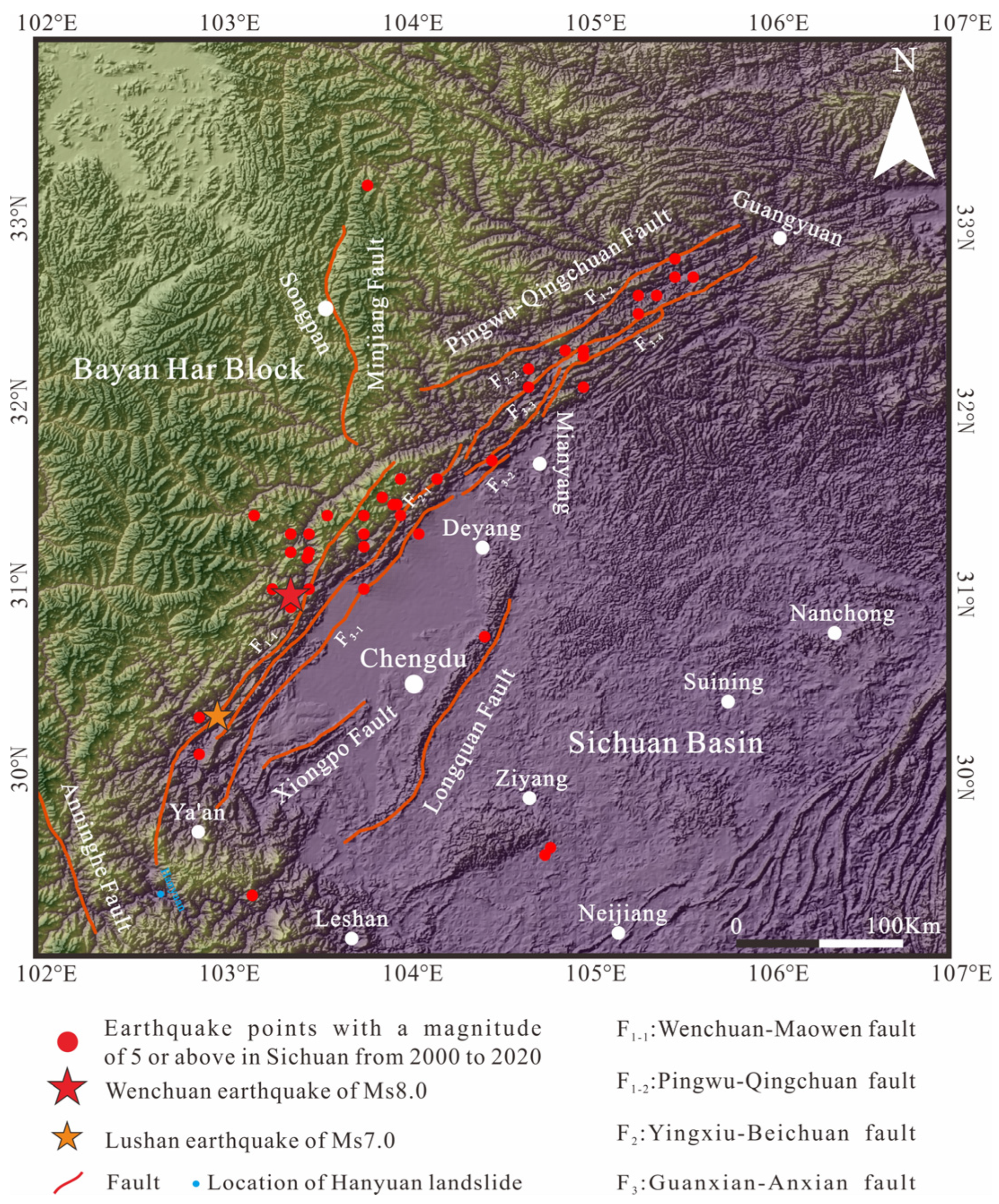
2.1. Regional Geological Background

Hanyuan County is located in the northern section of the Sichuan Yunnan north–south tectonic belt, with complex geological structures mainly controlled by three major tectonic belts: the NS-trending Hanyuan Zhaojue Fault, the Yiping Meigu Fault, the NE-trending Emeishan Fault, and the NW-trending Jinping Fault and Shimian Fault [18]. The topography is mainly mountainous, characterized by high in the northwest and low in the southeast, with the highest elevation of 4021 m, the lowest elevation of 550 m, and the maximum relative height difference of 3471 m. The climate of Hanyuan County is a subtropical monsoon humid climate, with an average annual temperature of 18.0 °C. According to Hanyuan County Meteorological Bureau statistics, the county’s annual average precipitation is 741.8 mm, and precipitation is mainly distributed in June to October, accounting for 74.6% of the annual precipitation. The area where Hanyuan landslide is a typical low- and middle-mountain slope landform, and the topography is in the shape of steps. The landslide is relatively steep, the average slope is 25°, and the steepest slope is 40°, which creates favorable topographic and geomorphological conditions for landslide instability. Figure 1 shows the main strata exposed in the study area (according to the 1:200,000 geological map), including Sinian (Z), Triassic (T), and Jurassic (J). The area where the landslide is located is the Neogene Pliocene Xigeda formation (N₂X). The lithology is mainly grayish yellow, dark gray sandstone, clay rock, and carbonaceous clay rock.

Affected by the recent continuous heavy rainfall, in the early morning of 21 August 2020, a landslide occurred in Group 6 of Zhonghai Village, Fuquan Town, Hanyuan County, Ya’an City. The amount of earthwork of the landslide was about 800,000 cubic meters, and the total volume of the landslide was about 5 million cubic meters, causing damage to public houses. Eight people are missing, one person was injured, and traffic on provincial highway 435 was interrupted. The investigation shows that the last continuous rainfall event before the landslide occurred from 19:00 on 18 August 2020 to 10:00 on 19 August 2020, and the cumulative rainfall in the past two weeks before the landslide occurred was greater than 260 mm. On the morning of 20 August, during the investigation of the hidden dangers of geological disasters in Hanyuan County, it was found that there were slope cracks and wrong ditches in Group 6 of Zhonghai Village, Fuquan Town. From 14:30 on the afternoon of the same day, 55 people from 14 households of the threatened masses were transferred by cadres of township and village groups. However, nine villagers were asked to evacuate that night and then returned privately, and they unfortunately suffered the disaster (Figure 2).

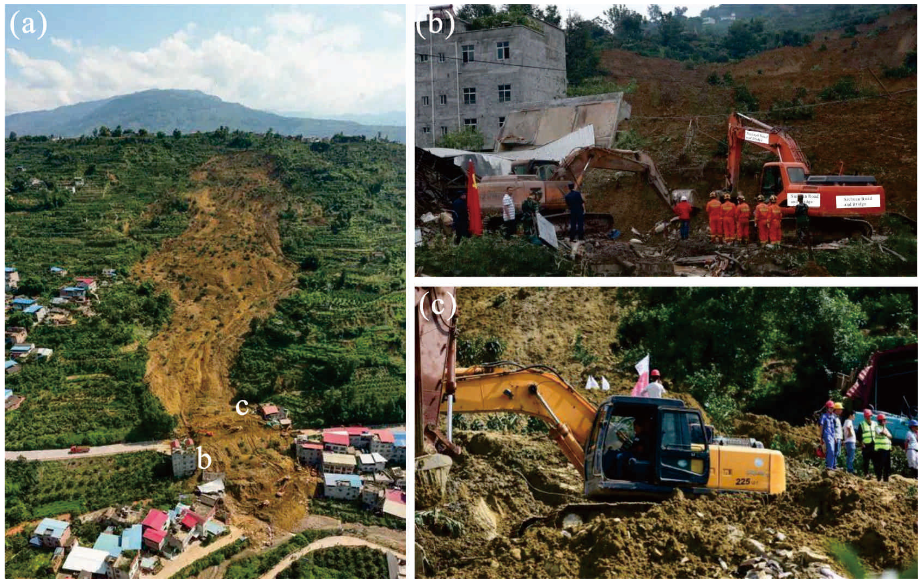
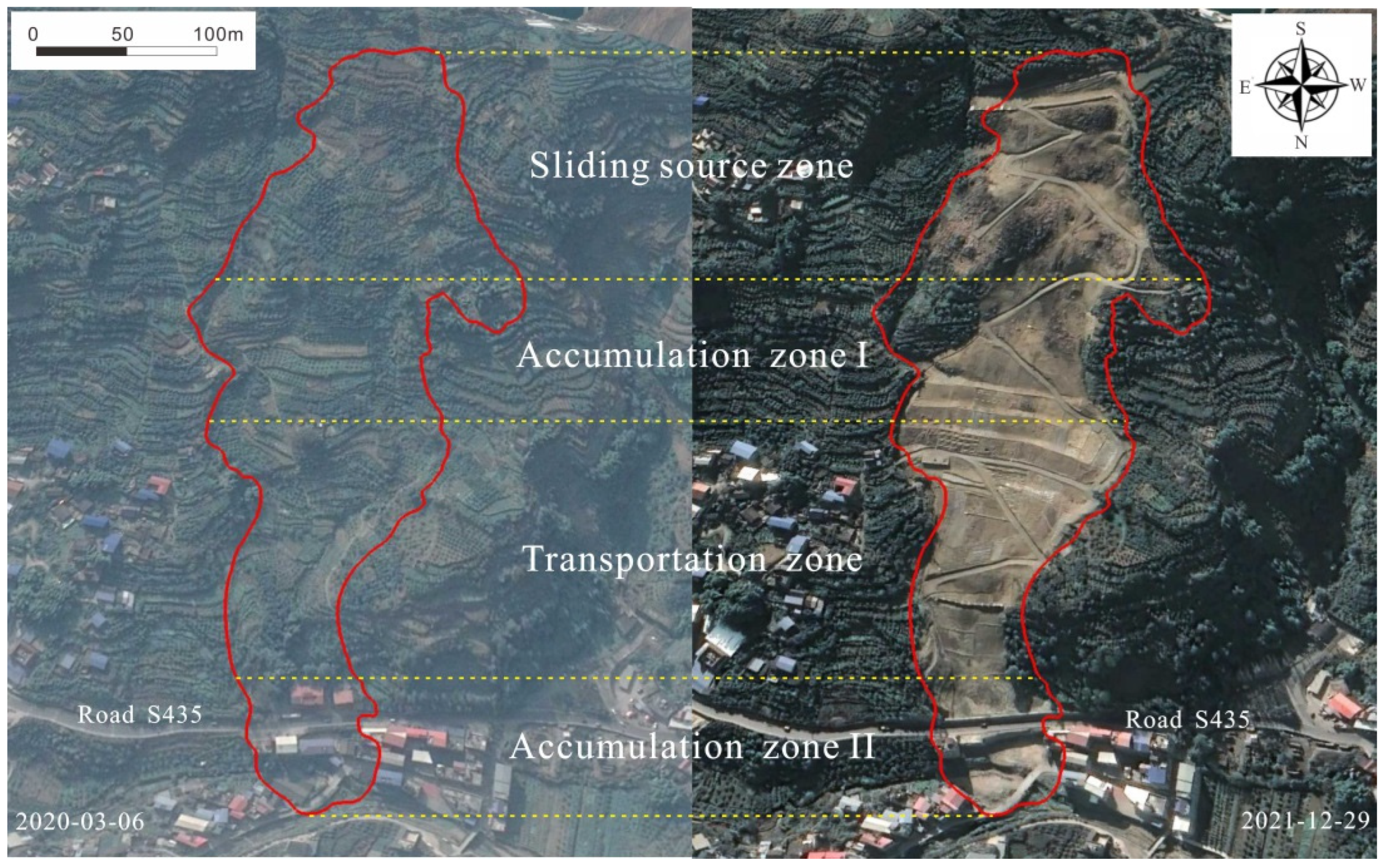
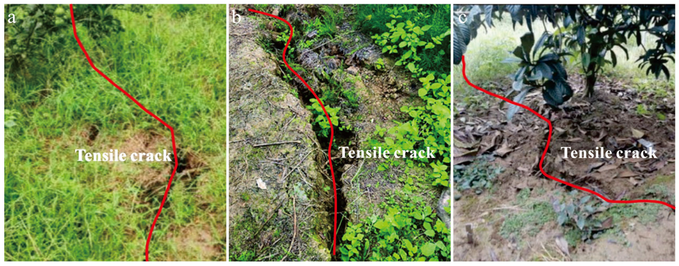
2.2. Landslide Zoning and Movement Accumulation Characteristics

Based on the field survey, the landslide is divided into four parts along the sliding direction: the sliding source zone, accumulation zone I, the transportation zone, and accumulation zone II (Figure 3).

2.2.1. Sliding Source Zone and Accumulation Zone I

The sliding source zone is covered with lush vegetation and loose Quaternary Holocene deposits. The main sliding direction of the landslide is NE9°, the width of the sliding source zone is about 200 m, and the slope angle is 60–80°. After the landslide, a typical “ring chair” landform was formed. The elevation difference of the back wall of the landslide is 6–8 m, and the occurrence is 10–355° < 45–55°. The elevation of the rear edge and front edge of the sliding source zone are 1035 m and 960 m, respectively. The rock and soil mass in the sliding source zone slide downward due to instability, and an obvious crack is formed at the rear of the landslide due to the effect of tension, with the extension direction of ES36° and WN38° (Figure 4b). Tensile cracks are also formed in the traction zone on the east and west sides of the sliding source zone. The strike of this fracture in the traction zone on the west side of the sliding source zone is NE25°, and the maximum width is about 20 cm (Figure 4a). The strike of this fracture in the traction zone on the east side of the sliding source zone is NE78°, and the maximum width is about 30 cm (Figure 4c). The maximum accumulation thickness in accumulation zone I is about 9 m. After the landslide, a residential house in accumulation zone I was completely buried, resulting in the loss of contact between two elderly people.

2.2.2. Transportation Zone

After one part of the landslide mass accumulates in accumulation zone I, the other part continues to slide downward, but the sliding direction is NE23°. This zone is a farming zone. Due to the influence of local residents’ farming activities all year round, the rock and soil mass are relatively soft. When the landslide mass slides downward at a high speed, the debris flow continuously scrapes loose rock and soil mass, causing the volume of the sliding mass to increase. At the same time, the scraping effect is gradually weakened due to the disintegration of loose deposits, mainly stacking, and the sliding direction changes again at an altitude of about 840 m due to the blocking of the terrain. The second accumulation is formed.

2.2.3. Accumulation Zone II

With the weakening of the debris flow energy of the sliding body, the sliding body begins to enter the accumulation zone. The elevation of accumulation zone II is 840–822 m. The accumulation zone II is a slope scarp above provincial highway S435, and the lower part is a residential area for villagers. In the downward sliding process, the debris fluid of the unstable sliding body is blocked by the buildings on both sides of the road and stops moving in front of the river. The accumulation direction of the final accumulation zone of the landslide mass is NW20°, the maximum horizontal distance along the accumulation direction is about 120 m, and the maximum accumulation thickness is about 6 m. The landslide is located in a terraced terrain, so the sliding distance of the sliding mass in the accumulation zone II is short, but it is very destructive, burying many houses.

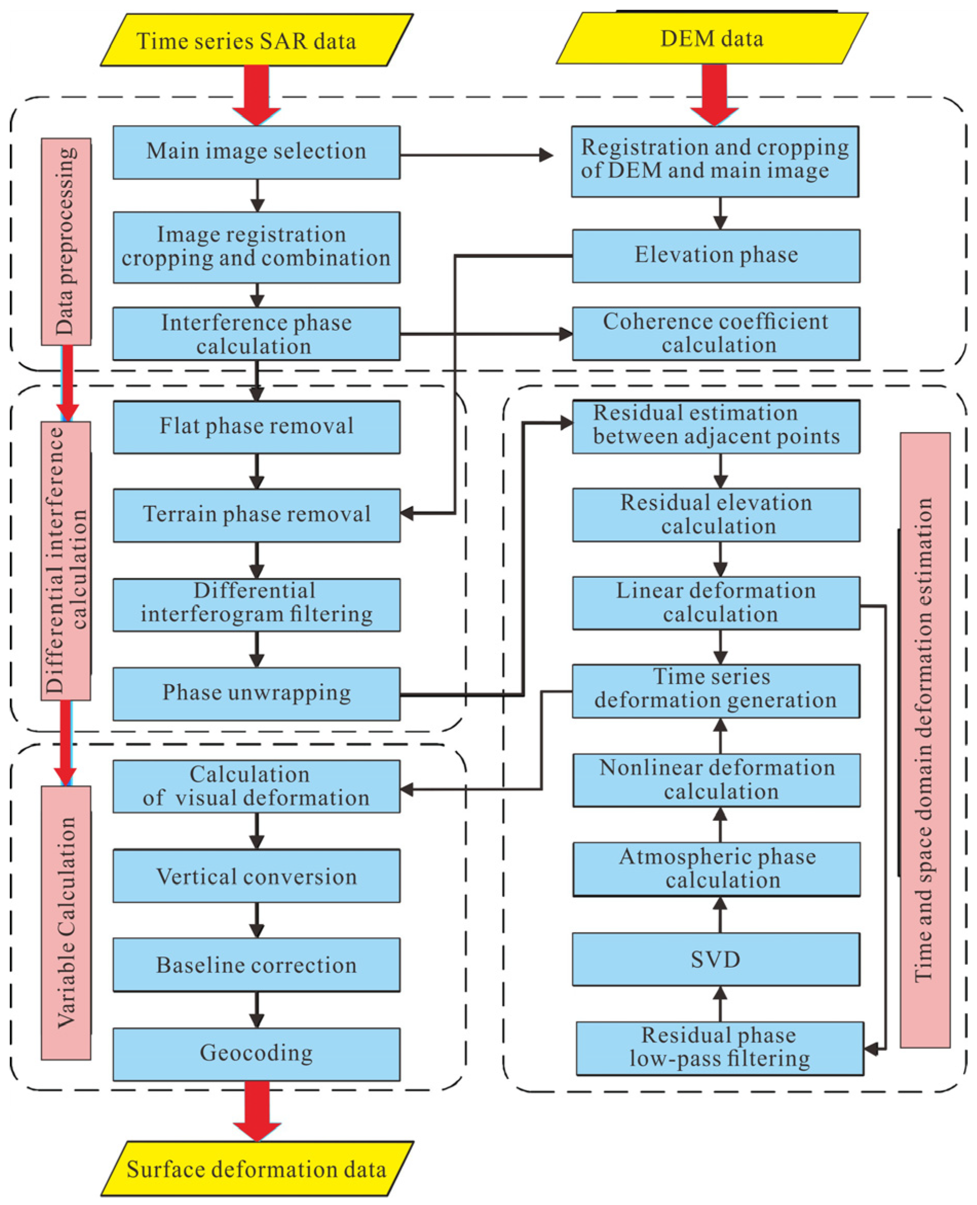
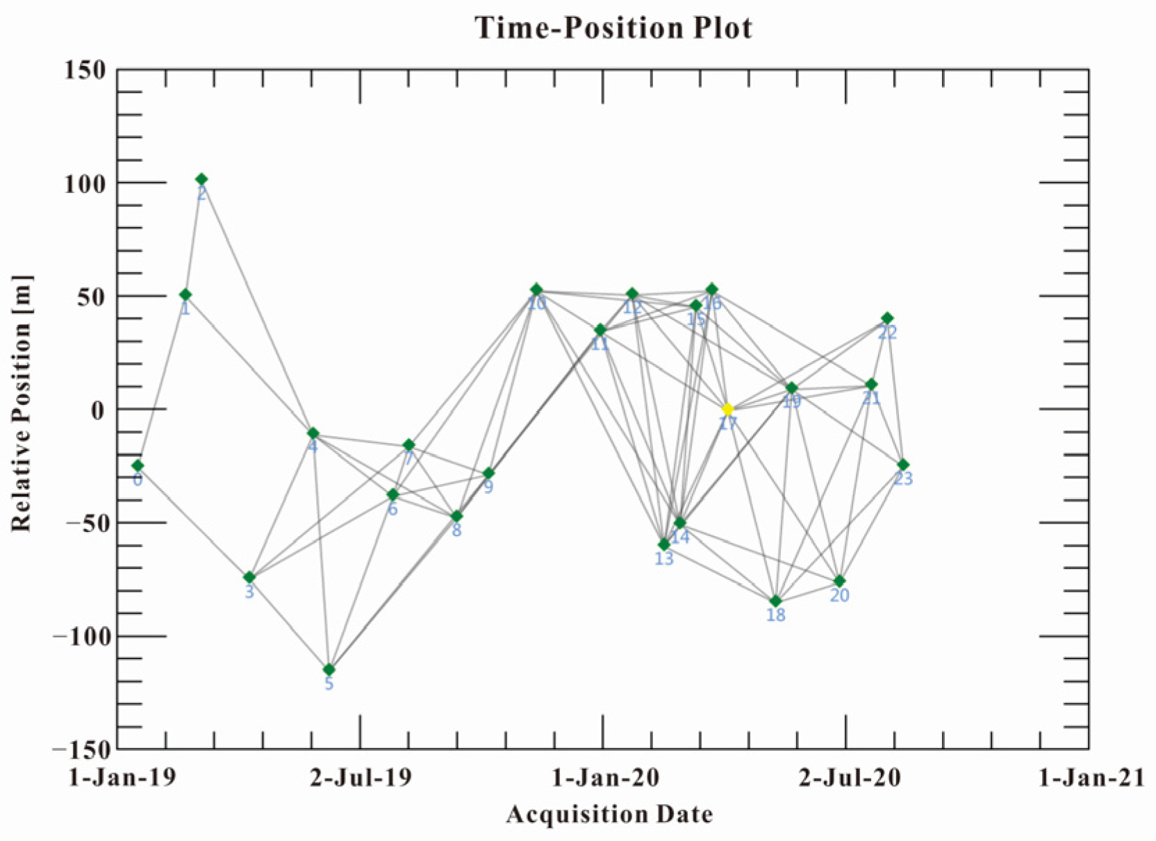
3. Data and Methodology

Time-Series Analysis

The basic idea of Small Baseline Subsets (SBAS) is to set a spatiotemporal baseline threshold, select high-quality interferograms to form one or more short baseline subsets, simulate terrain phases using DEM data according to the radar conformation equation, and then remove them from the radar interferograms. By utilizing the different characteristics of atmospheric delay and deformation in the time and space domains, the atmospheric delay phase is distinguished from the residual phase. For decorrelation and noise phase, multi-view methods are used to remove them. Finally, singular value decomposition (SVD) is used to estimate the deformation rate, and the average deformation rate is integrated in the time domain to obtain the value of historical deformation [19,20]. Firstly, assuming there are N + 1 SAR images of the same region obtained at time t0, t1, …, tN. Assuming that each image can interfere with at least one other image, this means that each short baseline subset is composed of at least two images. Based on the above assumptions, the number of generated interferograms is M, and it can be inferred that M satisfies the following inequality (assuming N is odd):

$${\displaystyle \frac{N+1}{2}}\le \mathrm{M}\le \mathrm{M}({\displaystyle \frac{N+1}{2}})$$

(1)

Assuming that the kth interferogram is generated from two SAR images obtained at time t_A and t_B, the terrain phase has been removed, and assuming t_B > t_A, in the azimuth distance pixel coordinate system (x, y), the interference phase of k at (x, y) can be expressed as

$$\delta {\Phi }_{\mathrm{k}}(\mathrm{x}, \mathrm{y})=\phi ({\mathrm{t}}_{\mathrm{B}}, \mathrm{x}, \mathrm{y})-\phi ({\mathrm{t}}_{\mathrm{A}}, \mathrm{x}, \mathrm{y}) \approx {\displaystyle \frac{4\pi }{\lambda }}[\mathrm{d}({\mathrm{t}}_{\mathrm{B}}, \mathrm{x}, \mathrm{y})-\mathrm{d}({\mathrm{t}}_{\mathrm{A}}, \mathrm{x}, \mathrm{y})]$$

(2)

In the formula, λ is the radar wavelength; D (t_B, x, y) and d (t_A, x, y) are the cumulative deformation values of the line of sight (LOS) relative to the reference time t₀ at time t_B and t_A, respectively. Therefore, d (t₀, x, y) = 0. Naturally, we can use d (t_h, x, y) h = 1, …, N to represent the deformation time series we want to obtain and set the corresponding phase as φ (t_h, x, y), Then, there are

$$\Phi ({\mathrm{t}}_{\mathrm{h}}, \mathrm{x}, \mathrm{y}) \approx {\displaystyle \frac{4\pi }{\lambda }}\mathrm{d}({\mathrm{t}}_{\mathrm{h}}, \mathrm{x}, \mathrm{y})$$

(3)

After unwrapping the phase signal, we can select a corrected pixel as a reference and represent its corresponding N unknown phase values as vectors:

$$\phi \mathrm{T}=[\phi ({\mathrm{t}}_1), \cdots , \phi ({\mathrm{t}}_{\mathrm{N}})]$$

(4)

The M values calculated from the differential interferogram are represented as vectors:

$$\delta \phi \mathrm{T}=[\delta {\phi }_1, \cdots , \delta {\phi }_{\mathrm{M}}]$$

(5)

Formula (4) can be defined using the following two vectors (HZ and HE correspond to the acquisition time series from the image and the main image in the image pair that generates the interferogram, respectively):

HZ = [HZ₁, ⋯, HZ_M]  HE = [HE₁, ⋯, HE_M]

(6)

The main image and the sub images are arranged in chronological order, i.e., HE_k > HZ_k, ∀k = 1, …, M, that is, the following equation:

$$\delta {\phi }_{\mathrm{k}}=\phi ({\mathrm{t}}_{\mathrm{Hek}})-\phi ({\mathrm{t}}_{\mathrm{HZk}}){\forall }_{\mathrm{k}}=1,\dots ,\mathrm{M}$$

(7)

The system of equations consisting of M equations with N unknowns is represented in matrix form as follows:

$$\mathrm{A}\phi =\delta \phi$$

(8)

We can perform SVD decomposition on equation system (8) as follows:

A = UZV^T

(9)

U is an M × M orthogonal matrix, with the first N rows being the eigenvectors of AAT, known as the left singular vector of A; V is an N × M unitary matrix, and all its rows are the eigenvectors of ATA, called the right singular vector of A; A is an M × N matrix, and its elements (singular values σ_h) are the square roots of the corresponding eigenvalues of the M × N matrix AAT. Usually, M > N, and there are M-N eigenvalues with 0. Moreover, due to the rank loss property of matrix A, there are L-1 additional zero eigenvalues, namely:

$$\mathrm{Z}=\mathrm{diag}({\sigma }_1, \cdots \cdots , {\sigma }_{\mathrm{N-L+1}}, 0, \cdots \cdots , 0)$$

(10)

Under the constraint of least squares, we can calculate the value of φ as follows:

$$\widehat{\phi }={\mathrm{A}}^{+}\delta \phi \hspace{1em}{\mathrm{A}}^{+}=\mathrm{V}{\mathrm{Z}}^{+}{\mathrm{U}}^{\mathrm{T}}$$

(11)

In the equation, Z⁺ = diag(1/$\sigma$₁, ⋯⋯, 1/$\sigma$_N-L+1, 0, ⋯⋯, 0); therefore:

$$\widehat{\phi }={\sum }_{\mathrm{h}=1}^{N-L+1}{\displaystyle \frac{\delta {\phi }^T{u}_i}{{\sigma }_i}}{\mathrm{V}}_{\mathrm{h}}$$

(12)

U_h and V_h are the row vectors of U and V, respectively, and the phase is converted to the average phase velocity:

$${\mathrm{V}}^{\mathrm{T}}=[{\mathrm{V}}_1{\displaystyle \frac{{\phi }_1}{t_1-t_0}}, \cdots , {\mathrm{V}}_{\mathrm{N}}={\displaystyle \frac{{\phi }_N-{\phi }_{N-1}}{t_N-t_{N-1}}}]$$

(13)

Thus, a new matrix equation is obtained: D_V = δφ; D is also an M × N matrix. For the k-th row, the column located between the acquisition times of the main and auxiliary images, D(k, k) = t_k+1 − t_k, Other D (k, k) = 0. In this case, applying SVD decomposition to matrix D yields the minimum norm solution of velocity vector V. Furthermore, starting with the composition of differential phase, we know that in addition to the contribution of deformation phase, there is also a phase contribution of elevation error Δq. Therefore, we can establish a system of equations:

$${\mathrm{D}}_{\mathrm{V}}+\mathrm{C}·\Delta \mathrm{q}=\delta \phi$$

(14)

On the basis of linear models, atmospheric phase and nonlinear deformation phase can be separated by appropriate filtering of residual phase in space and time. The main process of SBAS-InSAR method can be summarized as shown in Figure 5.

Therefore, in this study, SBAS is used to generate 82 differential interference pairs by setting a spatial baseline of 200 m and time baseline thresholds of 14 d and 35 d. Then, the singular value decomposition (SVD) is used to calculate the linear displacement velocity and elevation error, and the interference of atmosphere and noise phase is removed in the residual phase; thus, the deformation velocity and time series of coherent target points are obtained. In order to reduce errors and obtain more accurate deformation results, the interference threshold set in this study is 0.3, which reduces the error of phase unwrapping. The data set used in this study comes from the European Space Agency (ESA). The Sentinel-1 data set from 16 January 2019 to 14 August 2020 is used for SBAS time series analysis. The polarization mode is VV polarization, and the band is C-band. A total of 24 descent orbit data are selected, and in order to improve the orbit accuracy of Sentinel-1 images, the orbit error is corrected using POD Precise Orbit Ephemerides data. In addition, the SETM data with a resolution of 30 m released by NASA are used as external DEM data to remove the terrain phase of the interferogram. The interference combination of the selected Sentinel-1 dataset is shown in Figure 6.

4. Results

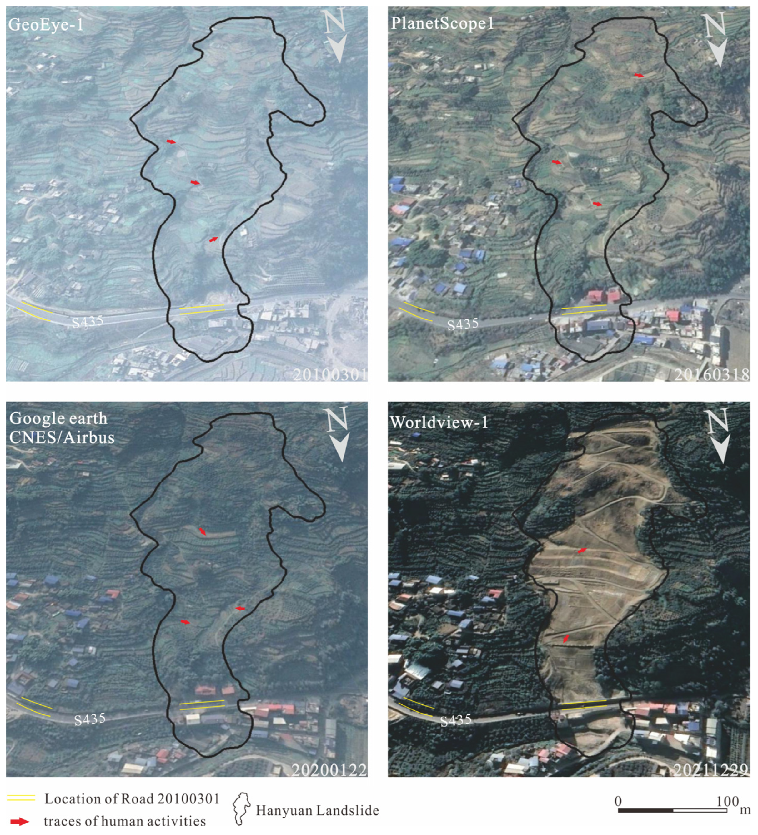
4.1. Geomorphological Changes Before and After Landslide

In this study, Geomorphic Change Detection (GCD) 7.0 software is used to extract the elevation changes before and after the landslide. The software can effectively distinguish the geomorphological changes caused by noise in DEM from the real geomorphological changes so as to detect geomorphological changes [21,22]. The DEM before the landslide is ALOS (Advanced Land Observing Satellite) 12.5 m DEM, and the DEM data after the landslide are obtained using a UAV. By resampling the DEM before and after the landslide to the same resolution, the elevation change map of the landslide is created, as shown in Figure 7. The elevation ranges from −17.4 to 8.7 m. The red area in Figure 7 represents the surface subsidence, the maximum elevation decreases by 17.4 m, the blue area represents deposition, and the maximum elevation increases by 8.7 m, indicating that the landslide has changed to a great extent before and after the collapse.

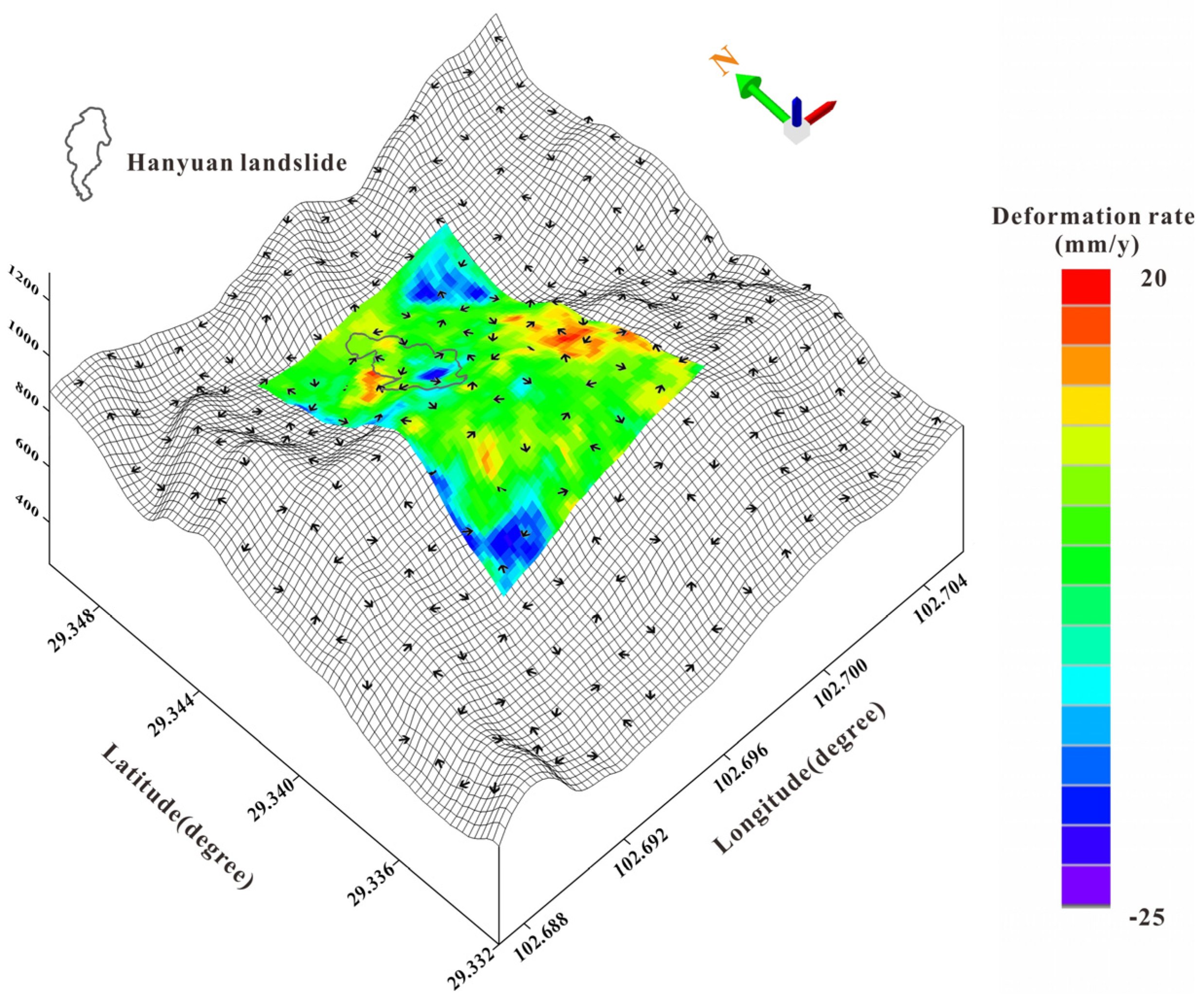
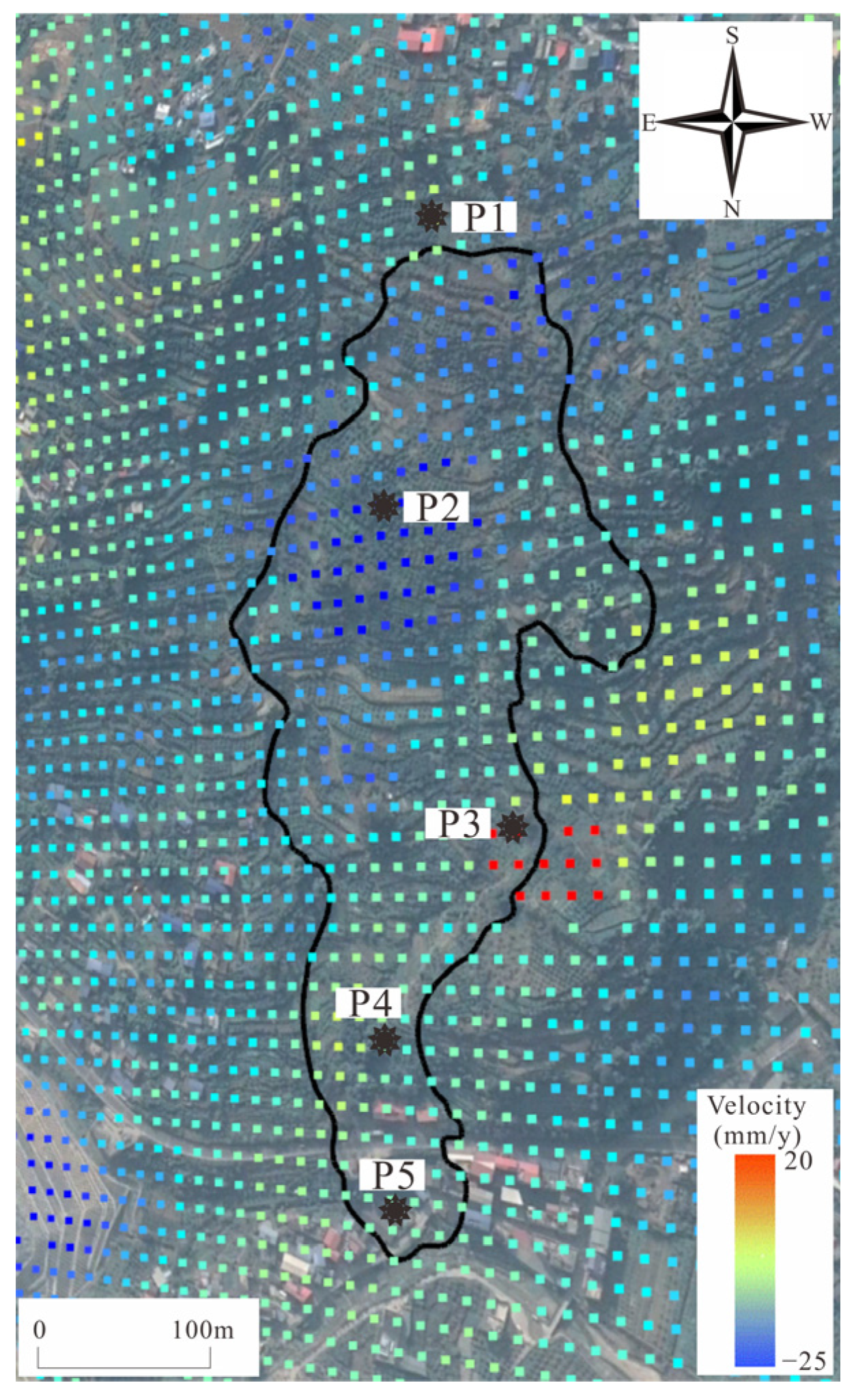
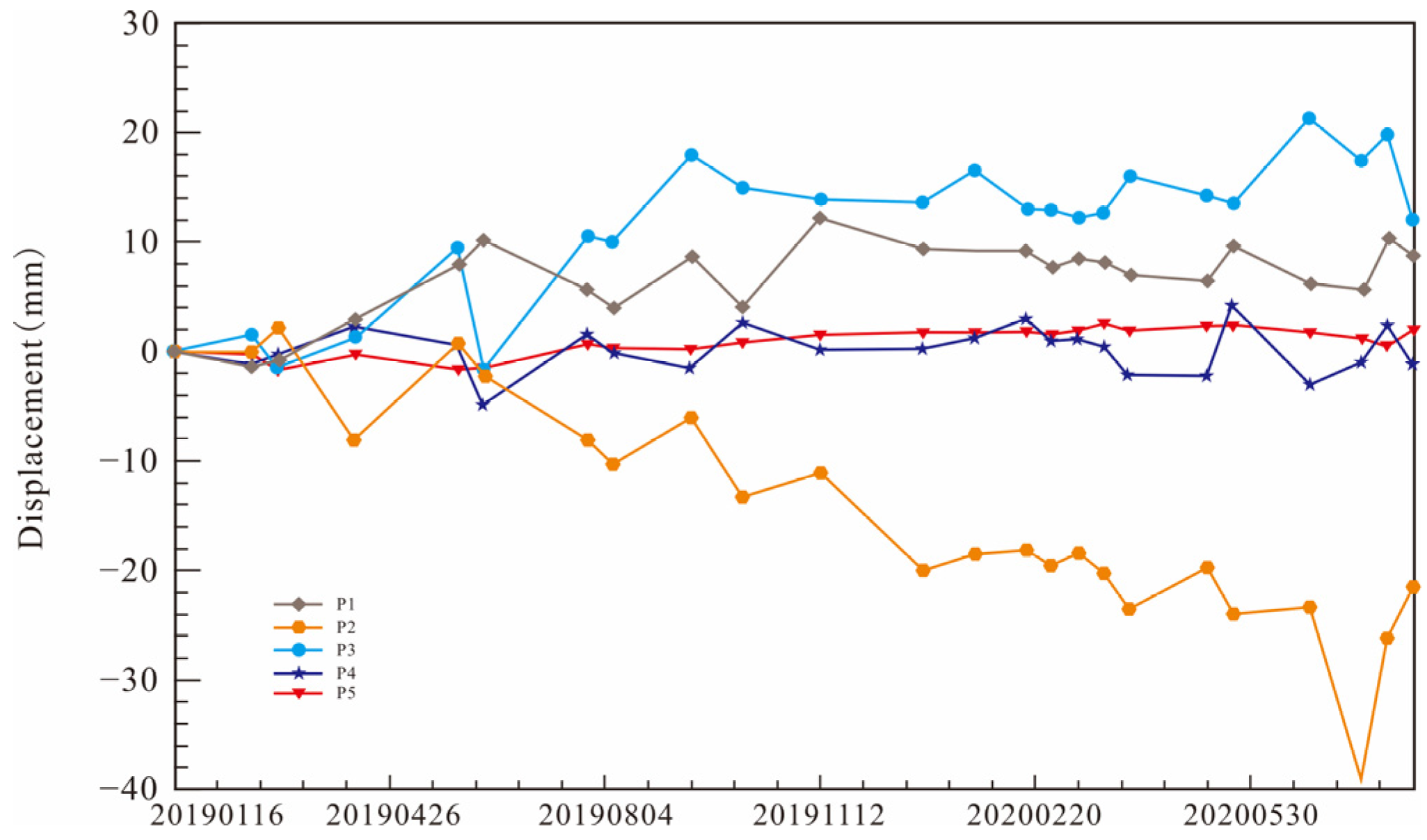
4.2. Deformation Evolution Process of Landslide

The SBAS-InSAR method was used to obtain the average line of sight (LOS) shape change rate map before sliding in the study area, as shown in Figure 8. It can be seen in Figure 8 that before the occurrence of the landslide, the upper part of the landslide deforms violently, and the maximum line of sight deformation speed was as high as 25 mm/a. There was an obvious uplift accumulation area on the right side of the landslide, and the maximum annual deformation rate was 20 mm/a. This may be caused by the compressibility of the soil in the upper and right areas. The disturbance results show that the Hanyuan landslide is in a state of continuous movement from January 2019 to August 2020. Based on these results, it is clear that InSAR technology can be used to identify unstable slopes in the early stages of monitoring and early warning so as to analyze post-disaster stability and reduce losses caused by secondary disasters.

4.3. Temporal and Spatial Evolution of Landslide

In order to explore the time evolution of the Hanyuan landslide, the five points shown in Figure 9 were selected for time series analysis. As can be seen in the pre-slip deformation velocity in Figure 10, the deformation velocity of P2 and P3 is relatively higher than that of other points, and the cumulative displacement of LOS at P2 reached near 40 mm. The analysis shows that the Hanyuan landslide has been in the process of deformation before failure, and the serious deformation area shows a linear growth trend.

5. Discussion

5.1. The Cause of Landslide

5.1.1. Rainfall

The Zhonghai Village landslide in Hanyuan County developed in the Xigeda Formation of the Neogene Upper Miocene. The bedrock of the landslide is mudstone, sandstone, and carbonaceous clay rock, with poor engineering properties of the rock mass. Its special interbedded mudstone and sandstone structure allows rainfall to fully infiltrate into groundwater. The landslide occurred about 40 h after rainfall, and rainfall data for approximately two weeks before the landslide disaster were collected from the local meteorological station, as shown in Figure 11. From August 7th to August 19th, there were 7 days with daily rainfall exceeding 10 mm, 4 days with daily rainfall exceeding 25 mm, and even heavy rainfall on August 16th and 18th, with rainfall reaching 70.6 mm and 76.2 mm, respectively. The cumulative rainfall in the two weeks before the landslide reached 263.6 mm. This short-term concentrated rainfall caused the groundwater level to rise sharply and caused soil moisture saturation, thereby reducing the shear strength of the soil and greatly increasing the instability of the slope. Rainfall seeps into the rocks through the upper layer of soil, gradually infiltrating the rock and soil mass. Once it exceeds the stability threshold, a landslide occurs. Therefore, the short-term heavy rainfall directly triggered the occurrence of the landslide.

5.1.2. Human Activities

Human activities have influenced the predisposing factors of landslides, as shown in Figure 12, and the traces of human activities are increasing. There are large areas of fruit trees and crops planted by local villagers on the slope, and there is also a natural pond not far from the landslide. In addition, villagers have excavated water channels to irrigate vegetation. The overflow and leakage of water channels and pools, as well as agricultural irrigation, can easily cause water flow to infiltrate the slope, increase the pore water pressure, soften rocks and soil, increase the slope bulk density, and thus promote or induce landslides. The rapid fluctuations in the water level of the pond increase the dynamic water pressure on the slope, which can also predispose landslides on the slopes and bank slopes. Unable to support excessive weight, losing balance, and sliding down along weak surfaces can predispose to landslides. Moreover, by monitoring the S435 road in historical images (2010–2018), it can be seen that the landslide has been in the creep stage. Human activities such as building railways, highways, and factories are also one of the main factors causing landslides in mountainous areas. According to the “Hanyuan County Annals (1986–2005)”, the S435 highway was built in 1942 and underwent reconstruction and widening in 1985 and 2002. Like most mountainous roads, S435 also uses a part cut part fill subgrade, which often poses safety hazards. Insufficient support for excavated steep slopes and inadequate compaction of the foundation can lead to foundation subsidence or sliding. Excavating the foot of the slope often causes the lower part of the slope to lose support and slide down. If the above-mentioned human effects are combined with unfavorable natural effects, it is more likely to promote the occurrence of landslides.

5.1.3. Earthquake

Earthquakes are also a predisposing factor for landslides. The Longmenshan Fault Zone is located at the junction of the North China Block, South China Block, and Qiangtang Block, with a length of about 500 km and a width of about 30–50 km. To the northwest is the Songpan Ganzi Ancient Residual Ocean Basin, and to the southeast is the stable Yangtze Craton. It extends in the NE-SW direction, and the fault sliding is mainly characterized by thrust with a right-handed strike–slip component. The main faults of the Longmenshan Fault Zone are distributed from west to east, including the Houshan Fault (Wenchuan Maoxian Fault), the Central Fault (Yingxiu Beichuan Fault), and the Qianshan Fault (Jiangyou Guanxian Fault) [23]. Affected by the overall stress background, the activity speed in this area is stronger than in other areas, making it prone to earthquakes, as shown in Figure 13. On 12 May 2008, a strong earthquake with a magnitude of 8.0 occurred in Wenchuan County, and on 20 April 2013, a strong earthquake with a magnitude of 7.0 occurred in Lushan. The magnitude of both earthquakes in Hanyuan County was 5. Two earthquakes accelerated the deformation process of the slope. Earthquakes are often accompanied by the activity of faults, which cause the rock layers on the slope to be displaced or broken, damaging the integrity of the rock layers and reducing their shear strength. In addition, earthquakes can further develop cracks in the rock mass on the slope, reducing its overall strength and stability, making it easier for the rock mass to slide under stress In addition, earthquakes can cause the upper surface of the slope to rise or the lower surface to settle, directly changing the overall slope of the slope and thus altering the stress distribution of the slope. In addition, the Sichuan Chongqing region experiences frequent rainfall in summer, leading to the occurrence of the Hanyuan landslide under the influence of multiple factors.

5.2. Comparison of SBAS-INSAR Technology Applications

As a widely distributed geological hazard, the study of the spatiotemporal evolution characteristics of landslides is of great significance for disaster warning and prevention [24,25].

Zheng used SBAS-InSAR technology to monitor the deformation characteristics of landslides in the Three Gorges Reservoir area, with a focus on analyzing the impact of reservoir water level fluctuations and rainfall on landslide activity. There is a significant correlation between landslide deformation and changes in the reservoir water level, and rainfall is an important factor triggering landslide activity. This study emphasizes the driving effect of hydrological factors (the reservoir water level and rainfall) on landslides [26]. Song et al. applied SBAS-InSAR technology to monitor landslide activity in high mountain areas of the Italian Alps, analyzing the impact of glacier retreat and freeze–thaw cycles on landslides. It was found that glacier retreat and freeze–thaw cycles significantly intensified landslide activity, and the deformation rate was closely related to temperature changes. The research focused on the driving mechanism of landslides due to climate factors such as temperature changes and freeze–thaw cycles [27]. Chirol et al. used SBAS-InSAR technology to monitor the deformation characteristics of landslides along the coast of California, USA, and analyzed the impact of sea level rise and seismic activity on landslides. It was found that the sea level rise and seismic activity significantly intensified landslide activity, and the deformation rate was positively correlated with earthquake frequency. Research focuses on the combined effects of seismic activity and sea level changes on landslides [28]. Wang et al. used SBAS-InSAR technology to study landslide activity in the Himalayan region, analyzing the driving effects of glacier melting and heavy rainfall on landslides. It was found that glacier melting and heavy rainfall are the main triggering factors for landslide activity, and the deformation rate significantly increases during the rainy season. Their study combines climate and hydrological factors to reveal the unique characteristics of landslides in high mountain areas [29]. Faisal et al. used SBAS-InSAR technology to monitor landslide activity in the Kyushu volcanic area of Japan and analyzed the impact of volcanic activity and rainfall on landslides. It was found that volcanic activity and rainfall jointly drive landslide activity, and the deformation rate significantly increases during the volcanic activity period and rainy season. Their study emphasizes the unique impact of volcanic activity on landslides [30]. All studies used SBAS-InSAR technology to successfully obtain high-precision deformation information of landslides and reveal their spatiotemporal evolution characteristics. Landslides in various regions exhibit obvious seasonal deformation characteristics, which are closely related to changes in climate or hydrological conditions. There are significant differences in the driving factors of landslides in different regions. The geological background varies in different regions, leading to different mechanisms of landslide evolution. The evolution time scale of landslides varies in different regions.

SBAS-InSAR technology has demonstrated strong application potential in the study of spatiotemporal evolution characteristics of landslides. Although there are differences in landslide driving factors and geological backgrounds in different regions, SBAS-InSAR technology can effectively capture the deformation characteristics of landslides and reveal their spatiotemporal evolution laws. Future research can further combine multi-source data (such as meteorological, seismic, and hydrological data) to improve the accuracy and timeliness of landslide warning while strengthening the comparative study of landslide evolution mechanisms in different regions, providing a scientific basis for global landslide disaster prevention and control.

6. Conclusions

In this paper, the spatiotemporal evolution process before the Hanyuan landslide is studied based on UAV images, a digital elevation model, and the Sentinel-1 data set. Firstly, the average rate and time series of the landslide along the radar line of sight were obtained by using SBAS-InSAR technology. The results show that the maximum average deformation rate of the landslide along the radar line of sight is 25 mm/a, the maximum cumulative displacement is close to 40 mm, and the deformation is unevenly distributed in space. Then, we used GCD software to extract the elevation changes of the terrain before and after the landslide. Finally, by analyzing factors related to rainfall, human activities, and earthquakes, it was inferred that the Hanyuan landslide was directly caused by short-term heavy rainfall under the influence of multiple factors. This study utilizes SBAS-InSAR technology to significantly enhance the ability of local governments to prevent and control landslides through high-precision and large-scale surface deformation monitoring. The application of this technology can not only reduce the losses caused by landslide disasters but also provide a scientific basis and technical support for local governments’ disaster prevention and reduction work.

References

1. Deng, Q.L. Slope Deformation Structure; China University of Geosciences Press: Wuhan, China, 2000; pp. 50–60. (In Chinese) [Google Scholar]
2. Iverson, R.M.; Logan, M.; Denlinger, R.P. Granular avalanches across irregular three-dimensional terrain: 2. Experimental tests. J. Geophys. Res. 2004, 109, F01015. [Google Scholar] [CrossRef]
3. Sun, H.Y.; Zhong, J.; Zhao, Y.; Shen, S.J.; Shang, Y.Q. The influence of localized slumping on groundwater seepage and slope stability. J. Earth Sci. 2013, 24, 104–110. [Google Scholar] [CrossRef]
4. Xu, Q.; Dong, X.J.; Li, W.L. Integrated Space-Air-Ground Early Detection, Monitoring and Warning System for Potential Catastrophic Geohazards. Geomat. Inf. Sci. Wu Han Univ. 2019, 44, 957–966. (In Chinese) [Google Scholar]
5. Malet, J.P.; Maquaire, O.; Calais, E. The Use of G lobal Positioning System Techniques for the Continuous Monitoring of Landslides: Application to the Super Sauze Earthflow (Alpes-de-Haute-Provence, France). Geomorphology 2002, 43, 33–54. [Google Scholar] [CrossRef]
6. Calcaterra, S.; Cesi, C.; Di Maio, C.; Piera, G.; Katia, M.; Margherita, V.; Roberto, V. Surface Displacements of Two Landslides Evaluated by GPS and Inclinometer Systems:A Case Study in Southerm Apennines, Italy. Nat. Haxards 2010, 61, 257–266. [Google Scholar] [CrossRef]
7. Zhao, C.Y.; Lu, Z.; Zhang, Q.; Juan, D.L.F. Large-area landslide detection and monitoring with ALOS/PALSAR imagery data over northern California and southern Oregon, USA. Remote Sens. Environ. 2012, 124, 348–359. [Google Scholar] [CrossRef]
8. Li, M.H.; Zhang, L.; Dong, J.; Tang, M.G.; Shi, X.G.; Liao, M.S.; Xu, Q. Characterization of pre- and post-failure displacements of the Huangnibazi landslide in Li County with multi-source satellite observations. Eng. Geol. 2019, 257, 105140. [Google Scholar] [CrossRef]
9. Yun, Y.; Lu, X.L.; Fu, X.K.; Xue, F.Y. Application of Spaceborne Interferometric Synthetic Aperture Radar to Geohazard M onitoring. J. Radars 2010, 9, 73–85. (In Chinese) [Google Scholar]
10. Liu, B.; Ge, D.Q.; Zhang, L.; Li, M.; Wang, Y. Application of ground-based radar interferometry technology in post landslide stability assessment. Geod. Geodyn. 2016, 36, 674–677+693. (In Chinese) [Google Scholar] [CrossRef]
11. Ashutosh, T.; Bihari, A.N.; Ramji, D.; Onkar, D.; Nagarajan, B. Monitoring of landslide activity at the Sirobagarh landslide, Uttarakhand, India, using LiDAR, SAR interferometry and geodetic surveys. Geocarto Int. 2020, 35, 535–558. [Google Scholar] [CrossRef]
12. Ma, S.Y.; Xu, C. The monitoring of a large ancient landslide in Sichuan Province, China, using interferometric synthetic aperture radar technology and sensitivity analysis in potential landslide mass modeling. IOP Conf. Ser. Earth Environ. Sci. 2021, 861, 052009. [Google Scholar] [CrossRef]
13. Wu, Y.Z.; Dong, Y.D.; Wei, Z.X.; Dong, J.H.; Peng, L.; Yan, P.; Ma, W.L. Genetic mechanisms and a stability evaluation of large landslides in Zhangjiawan, Qinghai Province. Front. Earth Sci. 2023, 11, 1140030. [Google Scholar] [CrossRef]
14. Mohsen, P.; Ali, M.; Saied, P.; Reza, D. Monitoring of Maskun landslide and determining its quantitative relationship to different climatic conditions using D-InSAR and PSI techniques. Geomat. Nat. Hazards Risk 2022, 13, 1134–1153. [Google Scholar] [CrossRef]
15. Qiao, N.; Duan, Y.L.; Shi, X.; Wei, X.F.; Feng, J.M. Study on the Early Warning Methods of Dynamic Landslides of Large Abandoned Rockfill Slopes. Appl. Sci. 2020, 17, 6097. [Google Scholar] [CrossRef]
16. Erin, L.; Regula, F.; Denise, R.; Lorenzo, N.; Lena, R. Multi-Temporal Satellite Image Composites in Google Earth Engine for Improved Landslide Visibility: A Case Study of a Glacial Landscape. Remote Sens. 2022, 14, 2301. [Google Scholar] [CrossRef]
17. Rajinder, B.; Gökhan, A.; John, D. Ground Investigations and Detection and Monitoring of Landslides Using SAR Interferometry in Gangtok, Sikkim Himalaya. GeoHazards 2023, 4, 25–39. [Google Scholar] [CrossRef]
18. Ge, Y.G.; Chen, X.C.; Fang, H.; Pei, L.Z. Studyonthe disaster of Dadu River fall occurred at Hanyuan County on August 6th. Mt. Res. 2009, 28, 123–128. (In Chinese) [Google Scholar]
19. Berardino, P.; Fornaro, G.; Lanari, R.; Sansosti, E. A new algorithm for surface deformation monitoring based on small baseline differential SAR interferograms. Trans. Geosci. Remote Sens. 2002, 40, 2375–2383. [Google Scholar] [CrossRef]
20. Yastika, P.; Shimizu, N.; Abidin, H. Monitoring of long-term land subsidence from 2003 to 2017 in coastal area of Semarang, Indonesia by SBAS DInSAR analyses using Envisat-ASAR, ALOS-PALSAR, and Sentinel-1A SAR data. Adv. Space Res. 2019, 63, 1719–1736. [Google Scholar] [CrossRef]
21. Wheaton, J.M.; Brasington, J.; Darby, S.E.; Sear, D.A. Accounting for uncertainty in DEMs from repeat topographic surveys: Improved sediment budgets. Earth Surf. Process Landf. 2010, 35, 136–156. [Google Scholar] [CrossRef]
22. Zhu, Y.R.; Qiu, H.J.; Yang, D.D.; Liu, Z.J.; Ma, S.Y. Pre- and post-failure spatiotemporal evolution of loess landslides: A case study of the Jiangou landslide in Ledu, China. Landslides. 2021, 18, 3475–3484. [Google Scholar] [CrossRef]
23. Wang, J.; Li, H.; Zhang, Y.; Li, H.P.; Li, Y.Z. Shallow crustal structure of the northern Longmen Shan fault zone revealed by a dense seismic array with ambient noise analysis. J. Asian Earth Sci. 2024, 276, 106338. [Google Scholar] [CrossRef]
24. Huang, C.; Hu, Q.; Cai, Q.; Li, M.Y. Post-earthquake spatiotemporal evolution characteristics of typical landslide sources in the Jiuzhaigou meizoseismal area. Bull. Eng. Geol. Environ. 2024, 83, 242. [Google Scholar] [CrossRef]
25. Yang, J.; Xu, C.; Jin, X. Joint Effects and Spatiotemporal Characteristics of the Driving Factors of Landslides in Earthquake Areas. J. Earth Sci. 2023, 34, 330–338. [Google Scholar] [CrossRef]
26. Zheng, Y.Z. Application of InSAR Technology in Landslide Monitoring in the Three Gorges Reservoir Area. Master’s Thesis, University of Geosciences, Beijing, China, 2019. (In Chinese). [Google Scholar] [CrossRef]
27. Song, K.S.; Li, L.; Tedesco, L.P.; Li, S.; Duan, H.T.; Liu, D.W.; Hall, B.E.; Jia, D.; Li, Z.C.; Shi, K.; et al. Remote estimation of chlorophyll-a in turbid inland waters: Three-band model versus GA-PLS model. Remote Sens. Environ. 2013, 136, 342–357. [Google Scholar] [CrossRef]
28. Chirol, C.; Haigh, I.; Pontee, N.; Thompson, C.E.; Gallop, S.L. Parametrizing tidal creek morphology in mature saltmarshes using semi-automated extraction from lidar. Remote Sens. Environ. 2018, 209, 291–311. [Google Scholar] [CrossRef]
29. Wang, D.D.; Chen, Y.H.; Hu, L.Q.; Voogt, J.A.; Gastellu, J.P.; Krayenhoff, E.S. Modeling the angular effect of MODIS LST in urban areas: A case study of Toulouse, France. Remote Sens. Environ. 2021, 257, 112361. [Google Scholar] [CrossRef]
30. Faisal, M.; Yu, T.; Gerrit, L.D.; Zhao, L.M.; Fan, C.; Elnashar, A.; Bashir, B.; Wang, G.K.; Li, L.L.; Naeem, S.; et al. Modeling Spatio-Temporal Land Transformation and Its Associated Impacts on land Surface Temperature (LST). Remote Sens. 2020, 12, 2987. [Google Scholar] [CrossRef]
Figure 1. A 3D geological map of the study area (revised according to 1:200,000 geological map).
Applsci 15 03872 g001
Figure 2. Photos of landslide site (102°41′45″ E, 29°20′44″ N). (a) Overview of landslide; (b) damaged houses; (c) accumulated soil.
Applsci 15 03872 g002
Figure 3. Comparison before and after landslide.
Applsci 15 03872 g003
Figure 4. Landslide crack. (a) The crack on the west side of the sliding source area has a strike of NE25 ° and a maximum width of about 20 cm. (b) The crack at the rear of the landslide extend in the directions of ES36° and WN38°. (c) The crack on the east side of the sliding source area has a strike of NE78° and a maximum width of about 30 cm.
Applsci 15 03872 g004
Figure 5. The SBAS-InSAR processing flow chart.
Applsci 15 03872 g005
Figure 6. Temporal and spatial baselines of Sentinel-1 orbit reduction data.
Applsci 15 03872 g006
Figure 7. Elevation difference before and after landslide.
Applsci 15 03872 g007
Figure 8. Diagram of average LOS deformation velocity of landslide (the arrow represents the aspect value).
Applsci 15 03872 g008
Figure 9. Average line of sight deformation speed of landslide.
Applsci 15 03872 g009
Figure 10. LOS displacement of landslide time series.
Applsci 15 03872 g010
Figure 11. Rainfall map of approximately two weeks before Hanyuan landslide.
Applsci 15 03872 g011
Figure 12. Multiple images contrasting the Hanyuan landslide (2010–2021).
Applsci 15 03872 g012
Figure 13. Regional structure and earthquake epicenter distribution map of Longmenshan Fault Zone.
Applsci 15 03872 g013
Disclaimer/Publisher’s Note: The statements, opinions and data contained in all publications are solely those of the individual author(s) and contributor(s) and not of MDPI and/or the editor(s). MDPI and/or the editor(s) disclaim responsibility for any injury to people or property resulting from any ideas, methods, instructions or products referred to in the content.