Learning Approach for Angle Estimation Based on Characteristics of Phase Drift

Abstract

Indoor positioning systems (IPSs) are increasingly vital for various applications on the Internet of Things (IoT), including home automation, navigation in large buildings, AR, and smart city development. These systems rely on techniques such as time of arrival (ToA), angle of arrival (AoA), and received signal strength indicator (RSSI), and Bluetooth low energy (BLE). Despite advancements, challenges such as signal fluctuations, multipath effects, and high infrastructure costs limit the accuracy and adoption of these systems. This paper proposes a deep neural network-based approach to enhance angle estimation by leveraging phase drift values, an underutilized aspect in current models. By employing the phase drift-dependent lightweight angle estimation (PLAE) model, we aim to improve angle prediction accuracy, particularly in complex indoor environments. Experimental results demonstrate that our model achieves higher accuracy compared to traditional methods. The integration of time series data handling capabilities in our approach highlights its potential to provide more reliable indoor positioning solutions. This research contributes to the development of specialized models for precise AoA estimation, addressing the gaps in existing methodologies.

1. Introduction

In response to the increasing demand for reliable indoor positioning systems (IPSs), a variety of techniques have been developed, including time of arrival (ToA) [1], angle of arrival (AoA) [2], and received signal strength indicator (RSSI) [3]. These methods employed some communication interfaces such as ultra-wideband (UWB) [4], Wi-Fi [5], and Bluetooth low energy (BLE) [6] to enhance the precision of indoor positioning [7,8]. However, the current generation of IPSs faces several challenges, including signal fluctuations, multipath effects, and high infrastructure costs, which collectively limit the accuracy and widespread adoption of these systems [9,10].

UWB offers centimeter-level accuracy and performs well in environments with minimal multipath interference. Nevertheless, the high cost and infrastructure requirements of this technology present considerable obstacles to its widespread adoption [11]. Wi-Fi-based positioning systems benefit from existing infrastructure and cost-effectiveness. However, these systems are susceptible to multipath effects and signal attenuation, which can impact the accuracy of the results obtained [12]. Bluetooth-based systems offer low power consumption and high compatibility with mobile devices; however, they are also prone to signal attenuation and multipath effects, which can affect the accuracy of the positioning results [13].

Despite the advancements in IPS, the accuracy of RSSI-based distance estimation methods is constrained by signal fluctuations, multipath effects, and environmental factors, particularly in complex indoor environments [7,10]. Significant progress has been made in developing AI and machine learning (ML) models for indoor positioning. The integration of AI-based models for Wi-Fi, BLE, and other wireless technologies led to notable improvements in the precision and robustness of indoor positioning systems [14,15,16]. However, research on AI models specifically designed for AoA estimation remains limited. The objective of this study is to utilize artificial intelligence (AI) for the precise prediction of AoA, particularly in complex indoor environments where traditional RSSI-based methods struggle due to instability and environmental factors. Conventional AoA estimation methods typically attempt to mitigate multipath effects, as these distortions are considered a primary source of error. However, in complex indoor environments, completely eliminating the multipath is often impractical. Instead, an alternative approach is to exploit these distortions as useful features rather than treating them as noise.

The need for accurate direction and angle estimation has been increased with applications such as smart glasses for gaze tracking, indoor navigation for the visually impaired, and augmented reality (AR) systems. Traditionally, RSSI has been more commonly used for distance estimation rather than angle [17]. However, with new use cases, the importance of AoA emerged. UWB using high-frequency signals, BLE, and Wi-Fi often faces significant challenges in maintaining precision in indoor environments due to fading and reflection.

Leveraging phase drift values, which have not been widely applied before, could improve precision. Phase drift occurs due to slight variations in the signal phase as it propagates. By accurately measuring these variations, AoA estimation accuracy can be enhanced. Incorporating machine learning techniques to analyze and interpret phase drift values offers a promising solution against the limitations of traditional methods.

This study aims to apply machine learning to identify features and perform angle estimation based on phase drift values. By exploring this approach, we aim to develop a phase drift-dependent lightweight angle estimation (PLAE) model that enhances the accuracy of AoA predictions in indoor settings, providing a more reliable solution compared to traditional methods. To date, no ML-based models effectively utilized phase drift for this purpose, highlighting the aspect of this research. This paper is structured as follows: Section 2 reviews related work in AoA estimation and indoor localization including ML approaches. Section 3 presents the proposed PLAE model, detailing its structure and algorithm. Section 4 discusses the experimental setup and results, demonstrating the model’s performance. Finally, Section 5 concludes the paper and suggests directions for future research.

2. Related Work

IPS significantly advanced with the integration of ML and deep learning techniques, addressing various challenges such as multipath effects, signal attenuation, and environmental interference. This section reviews various ML-based approaches for IPS, highlighting methods and technologies employed in different studies.

Recent research effectively utilized deep neural networks and ML algorithms to enhance BLE-based indoor positioning. To mitigate multipath-induced RSSI fluctuations, a fingerprinting technique using random forest was introduced in [18], achieving 96% accuracy. A comparative analysis of distance estimation using BLE in [19] integrated TX power into ML models, while a deep neural network-based approach in [20] combined RSSI and IQ components, achieving a localization accuracy of 70 cm, demonstrating robustness against changes in room content and AP configurations.

UWB is known for its fine delay resolution and obstacle penetration capabilities, making it ideal for indoor localization. A non-parametric ML regressor was applied in [21] to mitigate ranging errors directly in the physical layer, showing superior performance in real-world scenarios. Classification techniques such as support vector machine (SVM), random forest (RF), and multi-layer perceptron (MLP) in [22] effectively distinguished between line-of-sight (LOS), non-line-of-sight (NLOS), and multipath (MP) conditions. Furthermore, ref. [23] demonstrated that MLP and boosted decision trees (BDT) were effective for NLOS mitigation, particularly for mobile objects.

Wi-Fi technology is ubiquitous and widely used for indoor positioning. In [24], a Wi-Fi fingerprinting system using principal component analysis (PCA) [25] and various classifiers (KNN [26], decision tree [27], RF, and SVM [28]) improved localization accuracy while reducing computational costs. In [29], an approach combining relative and absolute RSS values mitigated device heterogeneity and RSSI variance, achieving a 0.87 m average localization error and reducing large errors by 30–50%. In [30], a method integrating kernel direct discriminant analysis (KDDA) [31] and relevance vector regression (RVR) [32] addressed RSSI-based inaccuracies, yielding notable accuracy improvements.

Traditional AoA estimation methods, such as multiple signal classification (MUSIC [33] and ESPRIT [34]), have been widely used due to their high resolution and computational efficiency. These algorithms leverage the spatial covariance matrix to estimate angles and have been extensively studied in theoretical research. While effective in many scenarios, their performance can degrade in complex indoor environments where multipath interference, phase noise, and low SNR conditions introduce challenges. AoA-based localization is particularly beneficial in indoor environments due to its high accuracy and independence from extensive infrastructure. Compared to RSSI-based fingerprinting and ToA methods, AoA provides robust positioning with fewer anchor nodes [35,36].

AoA estimation is a critical technique in indoor localization, offering high accuracy by determining the direction of incoming signals. In [37], a hybrid approach combining signal processing and machine learning trained regression models on snapshot data from multiple antennas, achieving at least 20% improvement over traditional MUSIC algorithms across various channel conditions. In [38], a convolutional neural network (CNN) was trained on the spatial covariance matrix’s eigenvectors, significantly outperforming MUSIC in low-SNR environments.

Despite advancements in AoA estimation techniques, there are relatively few machine learning models specifically designed to address this challenge, particularly those capable of handling the complexities introduced by phase drift. Most existing models fail to consider phase drift values, limiting their effectiveness in addressing fundamental issues such as multipath fading, which can significantly distort angle estimations. This gap underscores the necessity for specialized models that incorporate phase drift data to enhance AoA accuracy. The integration of time series data and positioning is crucial for accurate indoor localization, yet models designed specifically for precise angle estimation remain limited. The reviewed studies highlight the potential of using techniques such as GRU [39] and LSTM [40] to develop advanced models that leverage their time series handling capabilities, thereby improving AoA estimation accuracy.

3. Data Analysis and Model Construction

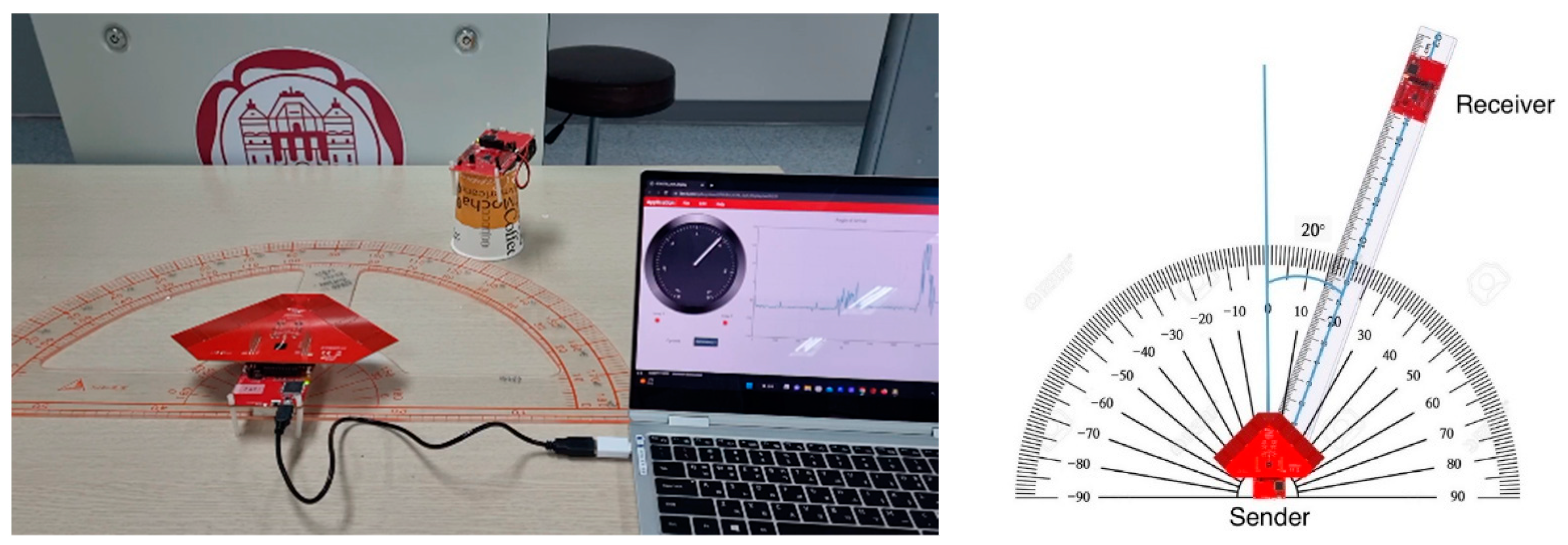
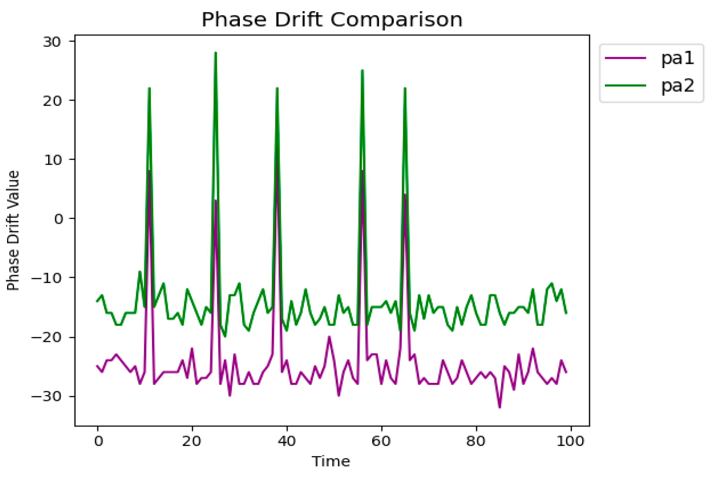
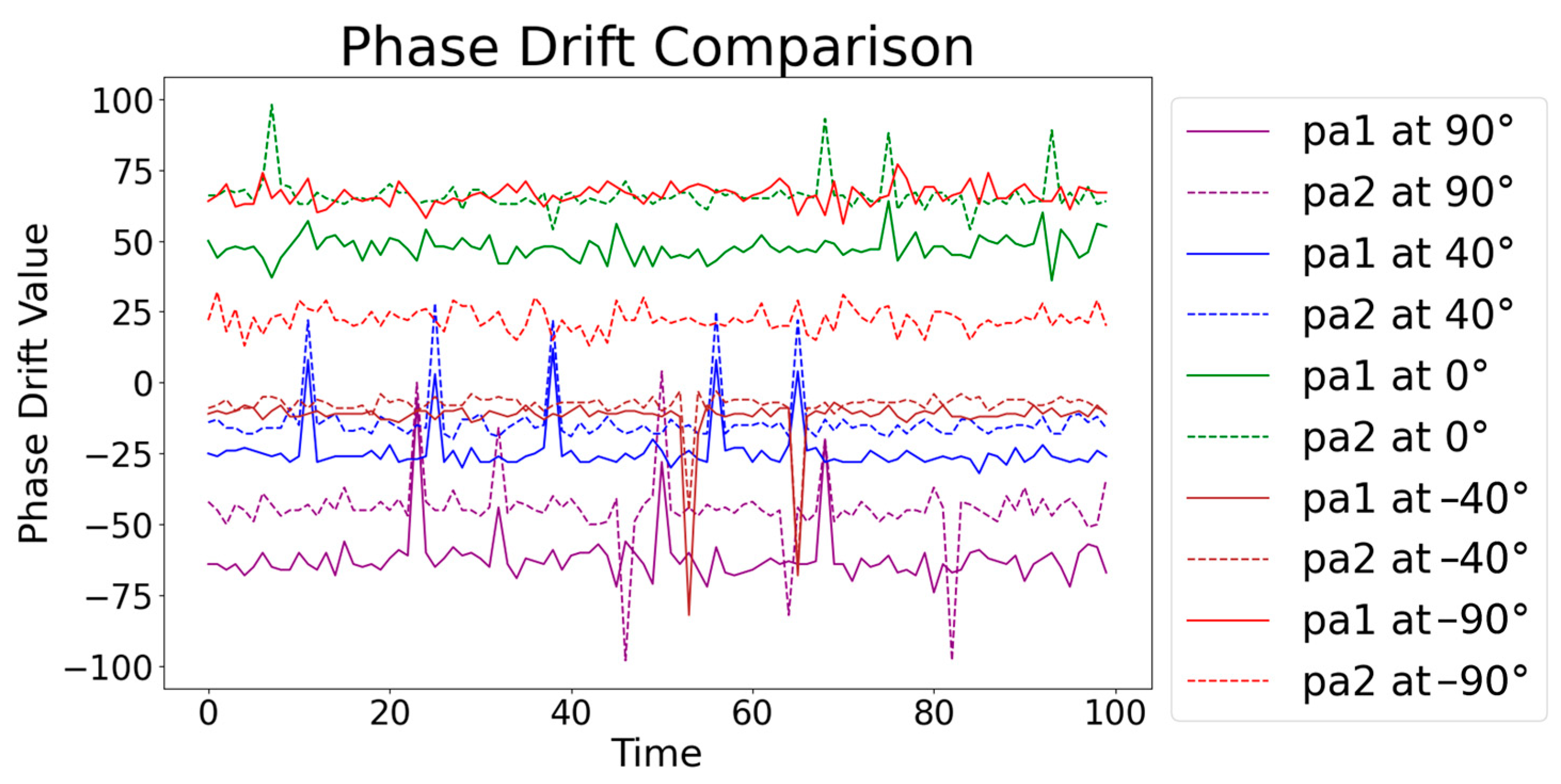
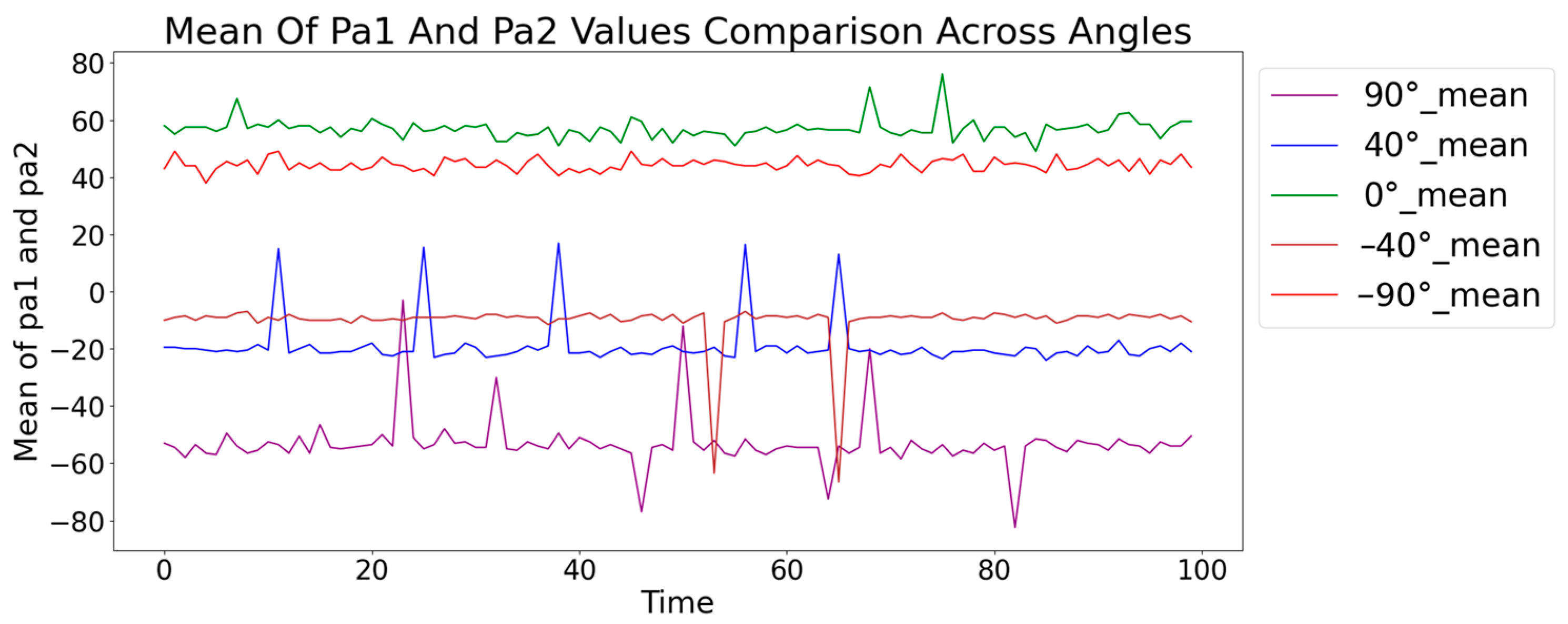
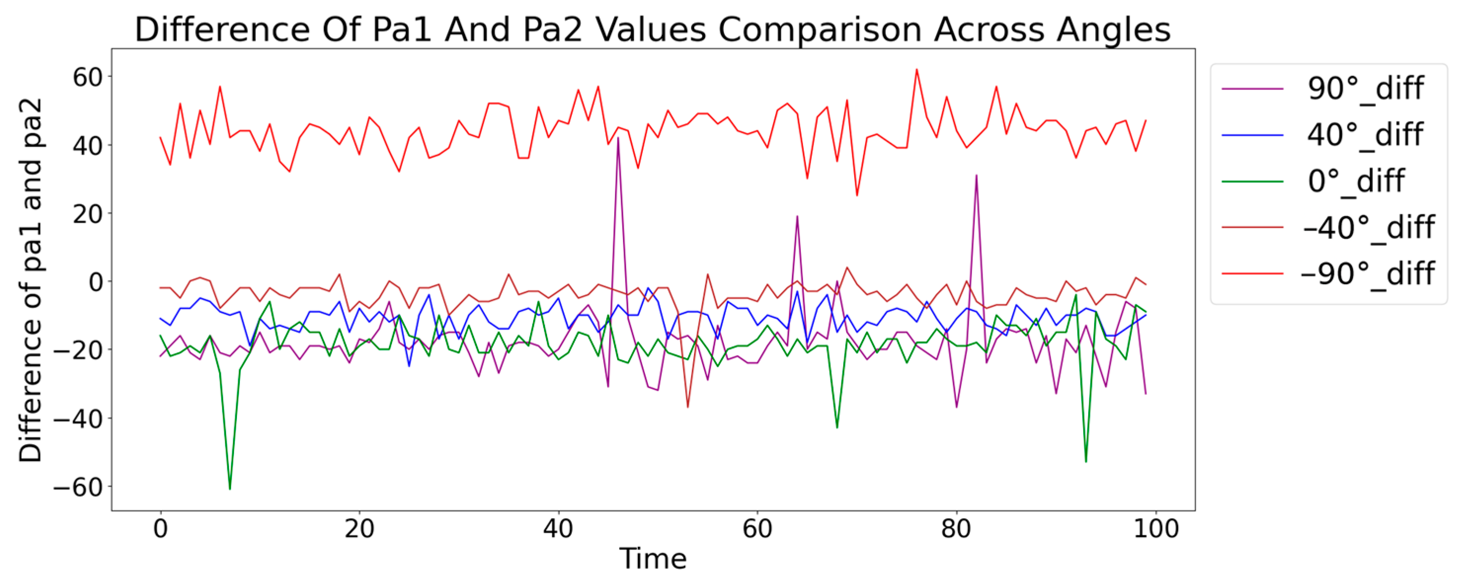
3.1. Radio Signal Analysis for Training Model

To collect the training data, we utilized the BOOSTXL-AOA kit [41] from Texas Instruments [42], as shown in Figure 1. The experimental setup involved securing the sender at a fixed location while rotating the receiver around it to collect data at precise distances, ensuring accurate angle measurements. The data collection was conducted indoors utilizing six antennas organized into two groups of three. Signals were gathered at 10-degree intervals, ranging from −90 to 90 degrees, with a signal interval of 625 μs. A Jetson Nano [43] was used for data acquisition, producing CSV files that included RSSI values, phase drift values (pa1 and pa2), and the corresponding AoA results. Each angle was measured approximately 20,000 times to ensure reliability.

Prior to data transformation, an in-depth examination of the phase drift values (pa1 and pa2 from antenna 1 and 2, respectively) was conducted to understand their characteristics and correlations. This analysis was essential to validate the use of the mean and difference between phase drift values as features in the regression model for angle prediction.

The phase drift values exhibited consistent patterns over time, indicating a strong correlation between them. As shown in Figure 2, when analyzing the phase drift values at a fixed angle (e.g., 90 degrees) over 100 time steps (each time step is 625 µs), although overall patterns are unstable, both phase drift values demonstrated similar trends. This correlation suggests that phase drift values are influenced by similar underlying factors. Consistent patterns highlight that the phase drift values are not random but have an underlying systematic behavior. The variations in phase drift values are likely due to the same environmental factors, such as multipath propagation, delay, reflection, fading, and refraction, which consistently affect the phase of the signals. The correlation between phase drift values indicates their potential to be effectively used together to improve the accuracy of angle estimation.

As shown in Figure 3, the comparative analysis of phase drift values across various angles revealed distinct patterns for each angle. For instance, dataset-40 shows phase drift values that are almost similar, while dataset-90 reveals a significant difference of about 50 units between phase drift values. This finding supports the hypothesis that phase drift values are angle-dependent and can effectively differentiate between different angles. The clear differentiation between the datasets at different angles highlights the phase drift values’ sensitivity to angular changes. The distinct patterns observed across different angles indicate that phase drift values can serve as reliable features for angle estimation, providing information that enhances the prediction accuracy in complex indoor environments.

To better capture these angle-specific features, the mean of phase drift values ((pa1 + pa2)/2) and the difference between phase drift values (pa1 − pa2) were calculated. Calculating the mean helps reflect the general trend and combined effect of phase drift values, while the difference captures the unique interaction and divergence between them, reflecting the nuanced variations due to different angles. As shown in Figure 4 and Figure 5, the mean and difference in phase drift values across different datasets provide insights into their angle-specific patterns. The analysis revealed that phase drift values for different angles exhibit distinct characteristics, which are better captured by considering their mean and difference. These observations underscore the importance of using both the mean and difference values to capture angle-specific features more effectively. This approach leads to improved model accuracy, as the unique patterns for each angle are more distinctly represented compared to using the raw data alone.

3.2. Learning Model Description

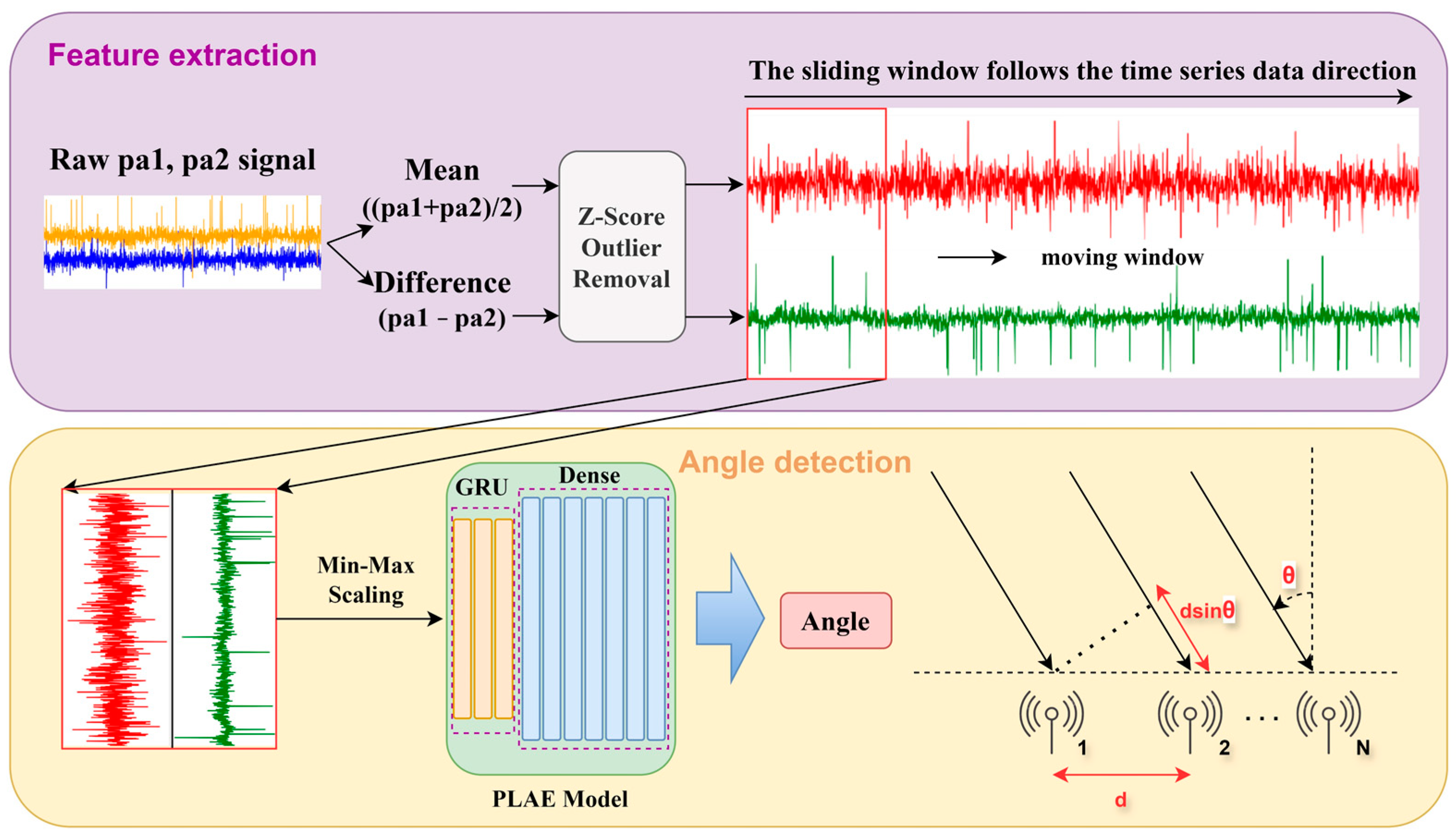
3.2.1. Preprocessing Analyzed Data

Data preprocessing involved several essential steps to ensure the dataset’s quality and suitability for training the regression model. Firstly, the phase drift values were processed to extract their means and differentiations. The mean values were calculated as (pa1 + pa2)/2, and the difference values were calculated as pa1 − pa2. As shown in Figure 6, the overall system overview of the PLAE model illustrates the processing of raw phase drift value signals through feature extraction and subsequent angle detection. This includes calculating the mean and difference values, performing Z-score outlier removal, and preparing the data for the model’s input layer. In Figure 6, the workflow of time series signal processing is further detailed, showing the structured sequences of 100 time steps using a sliding window approach, followed by min–max scaling and feeding into the model architecture, which comprises GRU and dense layers. This approach captures temporal dependencies and organizes the data for time series analysis.

To ensure the data were on a consistent scale, min–max scaling was applied to the dataset. Due to the different ranges of the mean and difference values, min–max scaling was applied separately to each. This normalization process is crucial for enhancing the performance and convergence of machine learning models by ensuring that all input features contribute equally to the model’s learning process. The scaled data were then divided into sequences, with the angle values serving as labels for each sequence. This structured approach enabled the segmentation of the dataset into training and testing sets, supporting effective regression analysis and model evaluation.

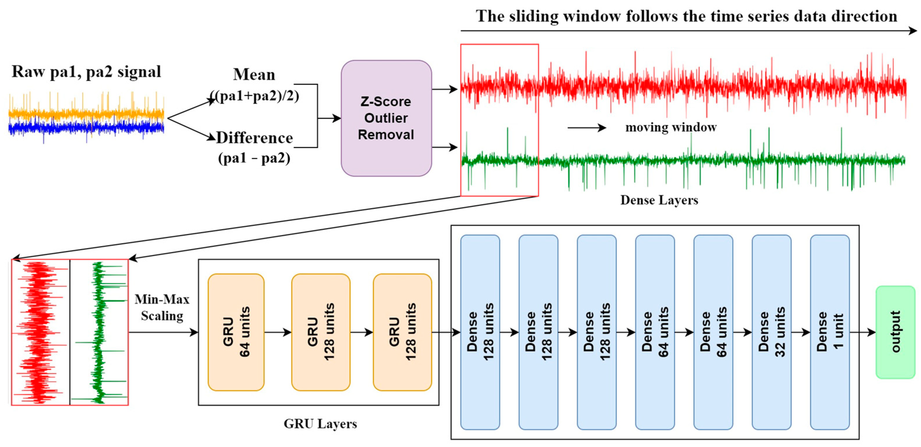
3.2.2. Model Construction

Traditional AoA estimation methods, such as MUSIC and ESPRIT, rely on the covariance matrix to determine the signal’s AoA. MUSIC estimates AoA by analyzing the eigenvalues of the covariance matrix R, using the pseudo-spectrum function:

$$P_{MUSIC}\left(\theta \right)={\displaystyle \frac{1}{a^H\left(\theta \right)E_n{E}_n^{H}a\left(\theta \right)}}$$

(1)

where $E_n$ represents the noise subspace and $a\left(\theta \right)$ is the array response vector. ESPRIT, on the other hand, estimates AoA by utilizing the shift invariance property of signal subspaces:

$$\widehat{\theta }=arc\mathit{sin}\left({\displaystyle \frac{\lambda }{2\pi d}}arg\left({\lambda }_i\right)\right)$$

(2)

where ${\lambda }_i$ is the eigenvalue obtained from the decomposition. These algorithms provide high accuracy but are sensitive to multipath effects and require high SNR conditions.

In contrast, this study proposes a deep learning-based model that directly learns AoA from phase drift variations. Unlike MUSIC and ESPRIT, which require explicit covariance matrix computations, our approach leverages time series patterns in phase drift using a GRU-based architecture. This enables robust AoA estimation even in low-SNR environments where traditional methods struggle.

The model construction phase aimed to design a framework capable of accurately predicting the angle from the preprocessed phase drift values. As shown in Figure 7, the model’s architecture comprised several key components, each tailored to handle the specific requirements of time series data and regression tasks.

The input layer was designed to accept sequences of N = 100 time steps, each containing the normalized mean and difference values of phase drift values. These input sequences were generated using a sliding window approach, where a fixed-length window moves across the time series data. Given a raw time series signal X = [$x_1$, $x_2$, …, $x_T$], the overlapping input sequences are constructed as follows:

$$S_t=\left[x_t,x_{t+1},\dots ,x_{t+N-1}\right]$$

(3)

where N represents the window size (100 time steps in this study), and $S_t$ represents the input sequence starting at time step $t$. The sliding window ensures that temporal dependencies are preserved while creating structured training samples. To ensure the input values were on a consistent scale, min–max scaling was applied to each feature. The transformation is defined as:

$$x^{\prime }={\displaystyle \frac{x-x_{min}}{x_{max}-x_{min}}}$$

(4)

where x is the original feature value, $x_{min}$ and $x_{max}$ are the minimum and maximum values in the training dataset, and $x^{\prime }$ is the normalized feature. This process ensures that all input values are within the range [0,1], allowing for stable model training.

After normalization, the sequential nature of the data was preserved using recurrent layers, which play a crucial role in capturing temporal dependencies. Although CNNs demonstrated strong performance in feature extraction, they are primarily designed for spatial data processing rather than temporal sequence modeling. AoA estimation relies on capturing the temporal dependencies in phase drift values, which CNNs are not inherently suited for. Therefore, we focus on recurrent models such as GRU and LSTM, which are explicitly designed for time series learning. Among recurrent architectures, we compared GRU and LSTM to determine the optimal model for AoA estimation. While LSTM utilizes three gates (forget, input, and output), GRU simplifies this by using only two gates (reset and update), resulting in lower computational complexity and faster inference times. The operation of the GRU can be mathematically described as follows:

• Update gate ($z_t$): determines how much of the previous hidden state to carry forward.

  $$z_t=\sigma (W_z·\left[h_{t-1},x_t\right]+b_z)$$

  (5)
• Reset gate ($r_t$): decides how much of the previous hidden state should be forgotten.

  $$r_t=\sigma \left(W_r·\left[h_{t-1},x_t\right]+b_r\right)$$

  (6)
• Current memory content (${h^{\prime }}_t$): calculates the new memory content based on the reset gate.

  $${h^{\prime }}_t=tanh\left(W_r·\left[{r_t·h}_{t-1},x_t\right]+b_h\right)$$

  (7)
• Final memory at time t: combines the previous hidden state and the current memory content.

  $$h_t=\left(1-z_t\right)·h_{t-1}+z_t·{h^{\prime }}_t$$

  (8)

GRU’s simplified architecture, with fewer gates compared to LSTM, allows for lower computational overhead while still capturing the necessary temporal dependencies for AoA estimation. In addition, Transformer-based models were also explored due to their self-attention mechanism, which enables effective long-range dependency modeling. However, AoA estimation primarily requires capturing short-range temporal dependencies in phase drift signals. The self-attention mechanism in Transformers increases computational cost while not necessarily improving accuracy for this task. Our comparative analysis confirmed that Transformers are less efficient than GRU in terms of both computational complexity and estimation accuracy. GRU layers were therefore employed to effectively learn sequential patterns in time series data, enabling the model to make accurate predictions based on historical phase drift values. Following the GRU layers, several fully connected (dense) layers were added to transform the learned temporal features into a suitable form for regression. The dense layers play a role in extracting angle characteristics from the processed data, identifying the complex relationships between input features that are necessary for accurate angle estimation. The mathematical operation in a dense layer is as follows:

$$y=W·x+b.$$

(9)

Each dense layer was followed by a ReLU activation function, introducing non-linearity into the model and enhancing its capacity to learn complex patterns from the data. The final layer of the model was a dense layer with a single unit, corresponding to the predicted angle. Since this was a regression task requiring continuous output values, no activation function was applied to this layer. Despite the data being collected at 10-degree intervals, the regression approach allowed the model to make precise predictions within these intervals, further demonstrating the model’s robustness and accuracy in angle estimation.

4. Performance Evaluation

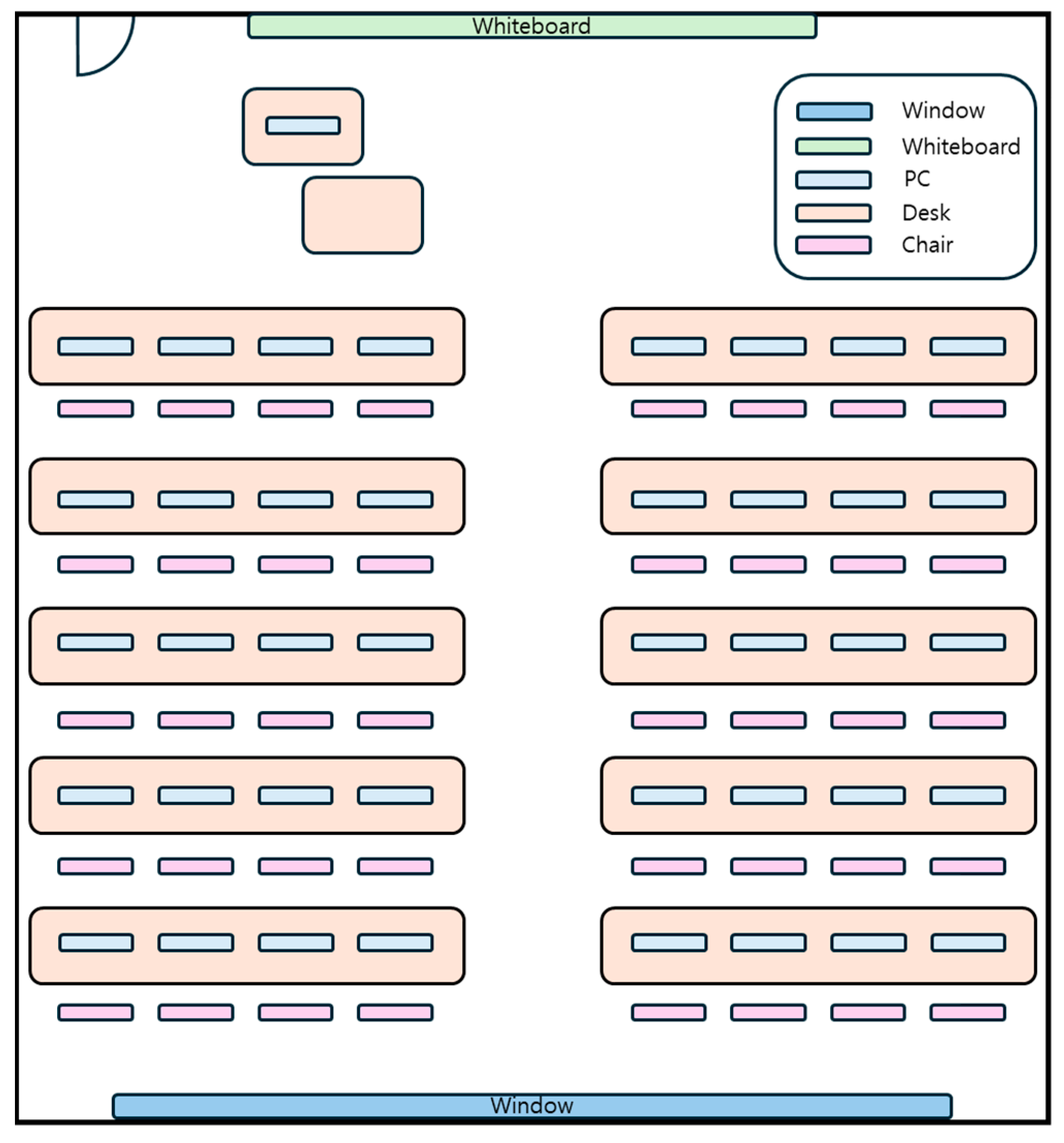
4.1. Training Environment and Data Composition

Figure 8 shows the university classroom where the experiments were conducted. The room measuring 201.36 m² contains 40 desks with PC. The room layout included rows of desks and chairs, which could act as minor obstructions, while the walls, whiteboard, and glass windows introduced reflective surfaces that could cause multipath propagation.

Due to the RS-232C serial communication’s speed limitation of 115,200 Baud rate, it was challenging to extract data in real time directly. To overcome this, we implemented a software function that first stores the data in internal memory. Once a specific data size is reached, the system pauses measurement and transfers the data to the host PC via RS-232C. This setup particularly emphasized pa1 and pa2, which were subsequently used to calculate mean and difference values for further analysis. The training environment, summarized in

Table 1. Server configuration for model training.

Component	Specification
CPU	Intel Xeon 4215, 64-bit, 8 cores, 16 threads
Memory	384 GB (64 GB × 6)
GPU	NVIDIA Quadro RTX 8000
GPU Memory	48 GB
TensorFlow	2.9.0
CUDA	11.2
CuDNN	8

, included specific hardware and software configurations to experiment model training and evaluation. Additionally, the training data and parameters of our model are described in

Table 2. Experimental dataset and model training parameters.

Class	Parameters	Configurations
Dataset	Total samples	379,995
	No. of antenna	6 antennas
	Antenna grouping	2 groups of 3
	Train:Val:Test	7:1:2
	Angle collection	10-degree intervals
	Signal interval	625 µs
Preprocessing	Length/window	100
	Input size	(100, 2)
	Min–max scaling	Yes
Learning	Learning rate	0.001
	Epoch	15
	Optimizer	Adam
	No. of GRU layers	3
	No. of dense layers	7
	Loss function	MSE
	Early stop	Yes
	Batch size	32

.

4.2. Outlier Removal

4.2.1. Outlier Definition and Detection

Outliers are exceptional data points that significantly deviate from the overall pattern of the dataset. These anomalies can arise due to various factors such as sensing errors, environmental interferences, or unexpected changes in the signal propagation path. In the context of IPSs, outliers can result from dynamic changes in the environment, such as the movement of obstacles, including people, which can cause sudden fluctuations in the received signal strength or phase drift values.

In this study, we identified outliers using the Z-score method, which calculates how many standard deviations a data point is from the mean of the dataset. Initially, a threshold of two standard deviations was tested but was found to be too sensitive, identifying an excessive number of data points as outliers. Subsequently, a threshold of three standard deviations was applied, which provided a more appropriate balance between sensitivity and the retention of valid data points for this dataset. The Z-score for a data point $x^i$ is calculated as follows:

$$Z_i={\displaystyle \frac{x^i-\mu }{\sigma }}$$

(10)

where μ denotes the mean of the dataset and σ denotes the standard deviation of the dataset. By applying this method to the phase drift values in the dataset, data points with Z-scores exceeding the threshold of 3 were flagged as outliers and subsequently analyzed to determine their impact on the model’s performance.

4.2.2. Impact of Outlier Removal

Outlier removal is a common practice to improve data quality and enhance the performance of machine learning models. However, the impact of outlier removal can vary depending on the nature of the data and the specific application. Additionally, it may undermine the intrinsic characteristics of the data. In this study, we analyzed the effect of outlier removal on the accuracy of angle estimation. The model was initially trained on the original dataset, which included all data points, encompassing potential outliers. This approach allowed the model to benefit from the representation of the indoor environment’s complexity, resulting in a certain level of accuracy. After outlier removal, the cleaned dataset, from which outliers identified by the Z-score method were removed, was used to retrain the model.

As shown in Figure 9, there is an improvement in the accuracy of the PLAE model predictions after outlier removal. The model trained on the dataset with outliers removed shows a closer alignment with the actual angles, as indicated by the more consistent proximity of the predicted values to the ideal line in the scatter plot. This suggests that outlier removal helped the model to generalize better by focusing on the most relevant patterns in the data, leading to a noticeable enhancement in prediction accuracy.

4.3. Analysis of Experiment Results

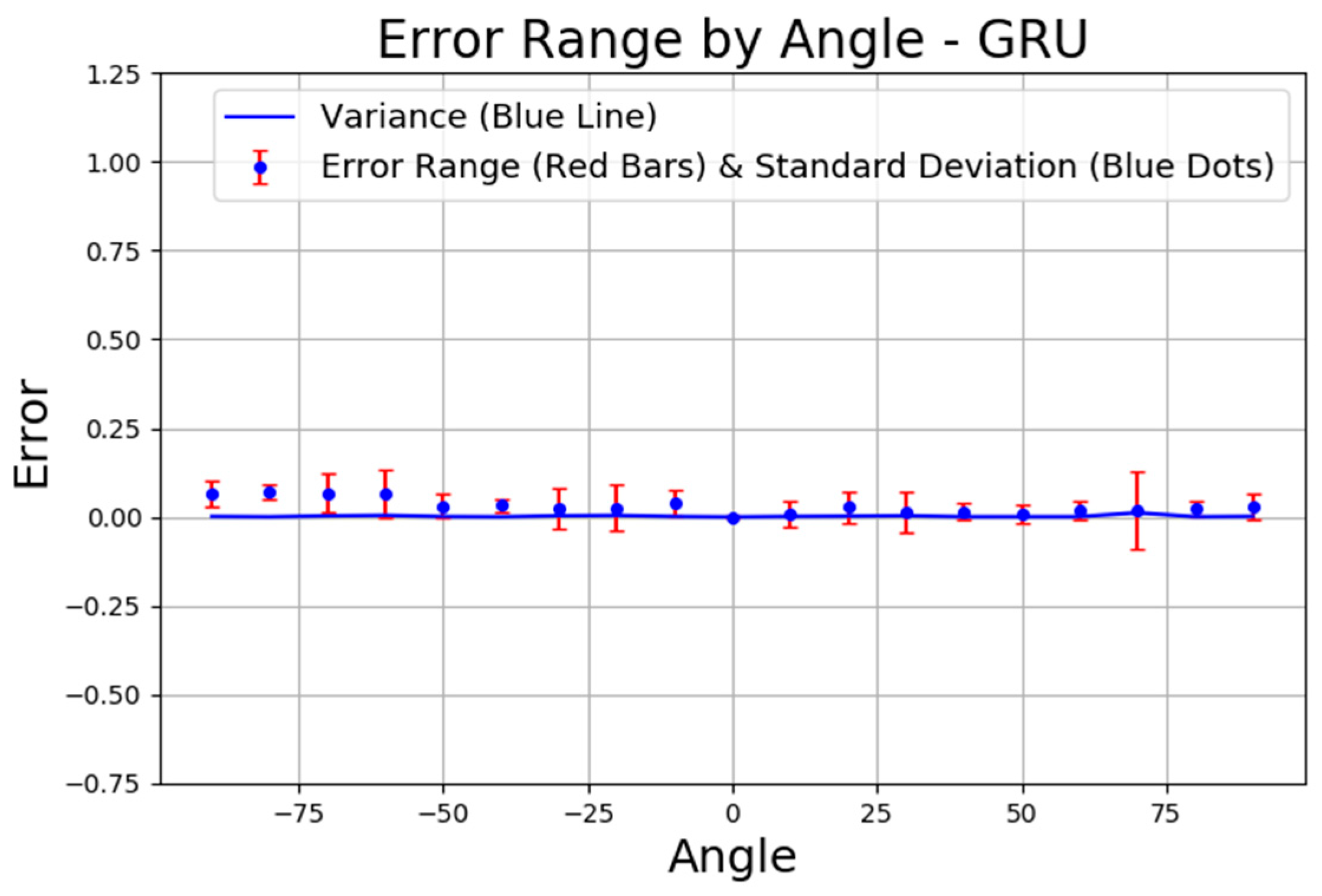
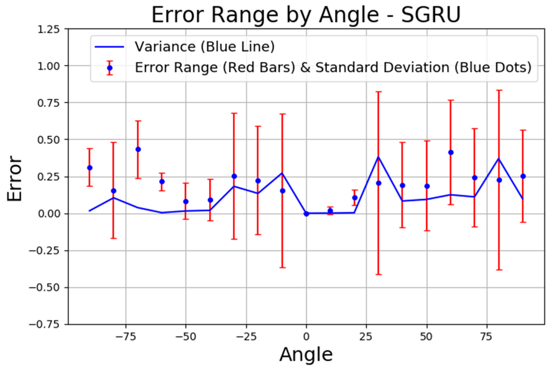
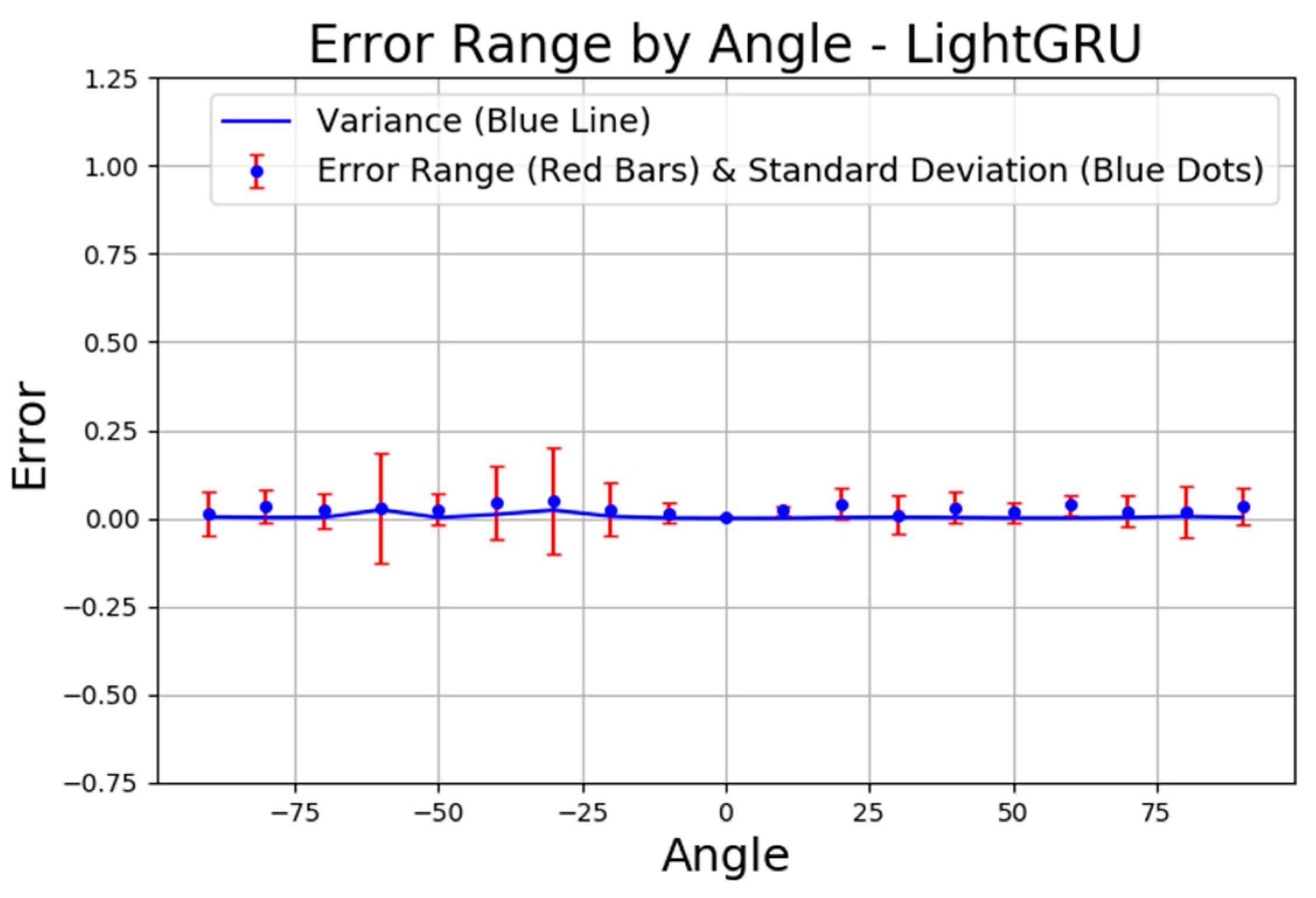
4.3.1. Accuracy of Angle

As shown in Figure 10, the relationship between the predicted and true angles for the test samples is illustrated, with the x-axis representing the true angles (degrees) and the y-axis representing the predicted angles (degrees). The blue dots represent the PLAE model predictions, while the orange dots represent the AoA predictions. The red dashed line indicates the ideal scenario where the predicted angles match the true angles. This visualization helps to assess how closely the model’s predictions align with the actual angles, highlighting the model’s accuracy in direction estimation. The PLAE model demonstrated a mean absolute error (MAE) of 0.031, which is significantly lower than the AoA’s MAE of 96.12. The maximum deviation from the true angles was 6.77 degrees for the PLAE model, whereas the AoA exhibited a much larger maximum deviation of 216.42 degrees. These metrics suggest that the PLAE model provides more accurate and consistent angle predictions compared to the AoA.

In open space environments where LOS is maintained, AoA typically performs well. However, in the measurement environment used in this study, obstacles, metallic objects, and various sources of interference such as propagation error, fading, and reflection adversely affect AoA accuracy. The AoA model operates by measuring the angle of arrival of signals, making it more susceptible to issues such as signal attenuation and multipath effects that are prevalent in indoor environments. As the angles move toward the extremes (i.e., closer to ±90 degrees), these effects become more pronounced, leading to greater prediction errors, as shown by the larger deviations in the orange dots away from the ideal line. These environmental factors can lead to significant errors in AoA estimation, as indicated by the scattered orange dots that deviate from the ideal line. Conversely, the PLAE model, represented by the blue dots, shows a closer alignment with the true angles, suggesting that the PLAE model is more robust to the environmental factors. The PLAE model can incorporate these errors as features, enabling it to provide more accurate angle predictions despite the complex indoor environment.

Figure 11 shows the evolution of the model loss during training and validation. The loss function used in this study is the mean squared error (MSE), which is defined as:

$$MSE={\displaystyle \frac{1}{n}}\sum _{i=1}^n{(y_i-{\widehat{y}}_i)}^2$$

(11)

where $y_i$ represents the true angle, ${\widehat{y}}_i$ represents the predicted angle, and $n$ is the total number of samples. The MSE measures the average squared difference between the true and predicted angles, with smaller values indicating better model performance. The unit of the loss is expressed in squared degrees (°²).

As observed in the graph, the training loss decreases significantly in the initial epochs and gradually stabilizes, indicating that the model is learning effectively. The validation loss follows a similar trend, decreasing consistently without sharp fluctuations. This suggests that the model is generalizing well to unseen data, with no significant signs of overfitting. The steady reduction in both losses implies that the model’s parameter updates are well-controlled, preventing abrupt changes that could destabilize validation performance. Additionally, the consistent trend in validation loss indicates that the distributional differences between the training and validation datasets are minimal. The dataset split in a 7:1:2 ratio appears to provide a balanced representation, reducing variability in validation performance. The smooth convergence of both losses suggests that the sliding window approach used for time series data does not introduce significant inconsistencies in capturing temporal dependencies. Overall, the model demonstrates stable learning dynamics, with validation loss aligning closely with training loss, indicating improved generalization and effective learning of underlying patterns.

Figure 12 illustrates the error distribution by angle for the GRU layer model. The x-axis represents the angle (degrees), while the y-axis represents the error values. The blue line in the figure represents the variance, which reflects the overall spread of prediction errors across different angles. The blue dots indicate the standard deviation at each angle, showing the typical amount of deviation from the mean error. The red vertical bars illustrate the error range, extending above and below the mean error to visualize how much the prediction errors can vary. This representation provides a comprehensive view of both the average deviation and the overall error distribution across angles. The results indicate that the error values are consistently low and stable across most angles, with minimal fluctuations. The variance remains close to zero, and the standard deviation is also low, suggesting that the GRU model provides reliable and consistent predictions across different angles without significant deviations or spikes.

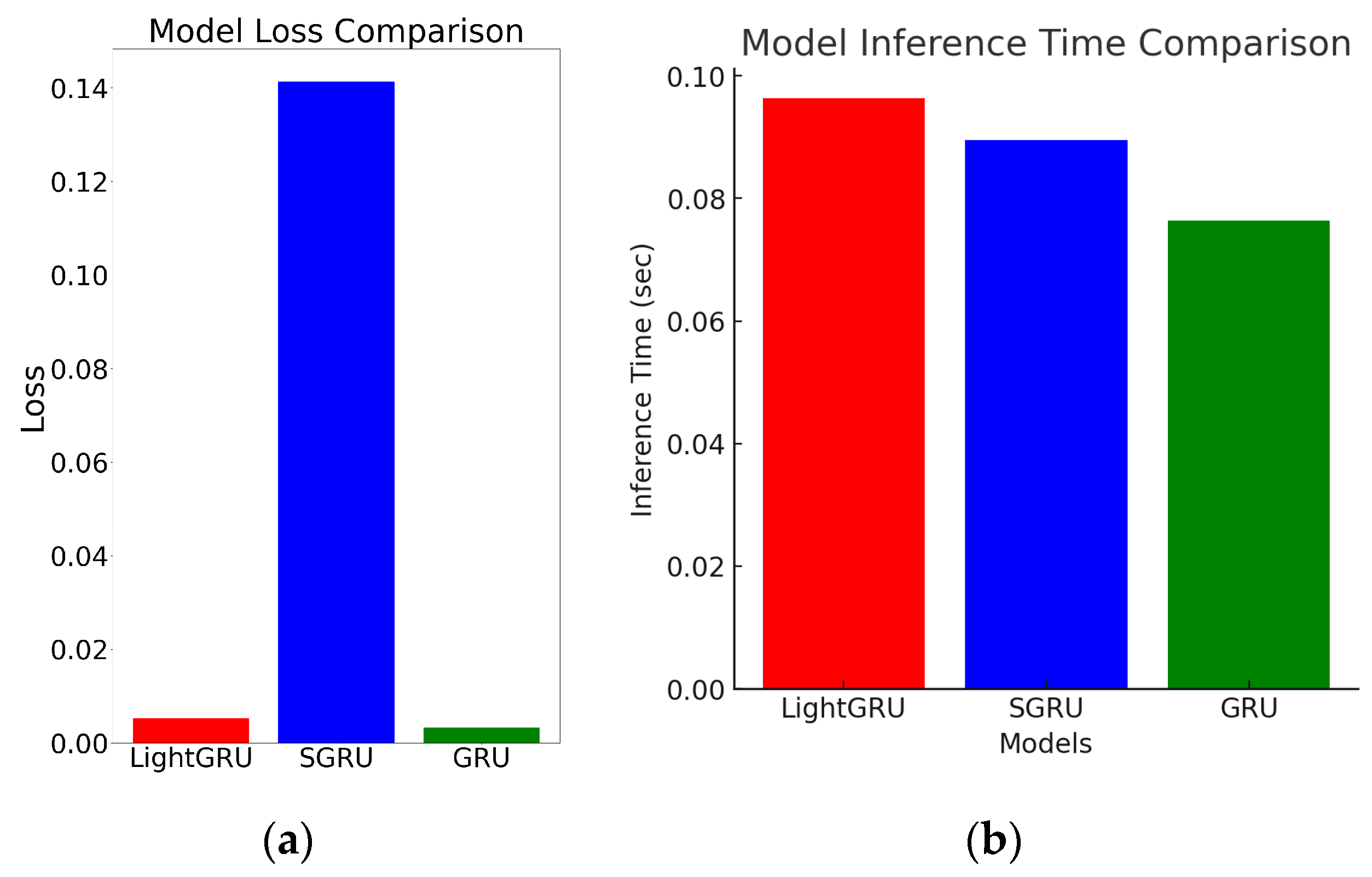
4.3.2. Computation Cost Evaluations

To determine the most suitable model architecture for angle estimation, we conducted extensive experiments comparing different neural network structures, including both recurrent-based models (LSTM, GRU) and Transformer-based models. Our experimental results demonstrate that GRUs provided the best balance between accuracy and computational efficiency, making them the most suitable choice for real-time angle estimation in resource-constrained environments. Compared to LSTM, which required 311,617 parameters with a validation MAE of 0.0513, the GRU model achieved a lower MAE of 0.031 with fewer parameters (250,689), making it a more efficient alternative.

Unlike LSTM, which consists of three gates (forget, input, and output), GRU uses only two gates (reset and update), reducing computational complexity. This structural difference allows GRU to perform faster training and inference while maintaining comparable accuracy. Additionally, the Transformer model, while lightweight (35,565 parameters), exhibited higher MAE (1.3103), indicating poorer accuracy in angle estimation. While Transformer-based models are highly effective in capturing long-range dependencies, they may not be the optimal choice for AoA estimation. Unlike natural language processing tasks where attention-based mechanisms excel, AoA estimation relies heavily on local temporal dependencies in phase drift signals. Recurrent-based models, such as GRU, are inherently more suited for such tasks, as they efficiently capture sequential patterns over time.

Simplified gated recurrent unit (SGRU) [44] and LightGRU [45] are variants of the GRU designed to reduce computational complexity. SGRU simplifies certain computations of the original GRU, maintaining its advantages while offering faster computation due to a more lightweight design. LightGRU, on the other hand, adopts an even more streamlined structure to facilitate efficient operation in resource-constrained environments such as embedded systems. This model aims to minimize computational cost without compromising GRU’s performance. The key differences between these models and the original GRU lie in their architecture. SGRU reduces the number of computations by merging or removing specific parameters and gates, which results in faster operations. LightGRU goes further by reducing the parameter count or simplifying computational processes, making it particularly suitable for embedded systems. Therefore, we also applied both the SGRU and LightGRU to our experiments to evaluate their performance in enhancing angle prediction accuracy compared to traditional GRU.

In Figure 13, the SGRU layer model’s error distribution by angle shows more variability compared to the GRU layer model shown in Figure 12. The standard deviation is significantly larger in multiple angular regions, particularly around ±75°, ±25°, and near 0°. Additionally, the variance, represented by the blue line, shows multiple spikes throughout the angle spectrum. This suggests that the SGRU layer model’s performance is less stable overall, with more pronounced prediction errors at various angles. One potential reason for this behavior is the impact of multipath reflections in the indoor environment. The experimental setup includes multiple desks, chairs, walls, and a whiteboard, which can cause signal reflections and diffractions, introducing phase distortions at specific angles. Notably, the regions around ±75° and ±25° are more exposed to these environmental structures, likely increasing signal interference effects. Since the same dataset was used for training all models, the higher variability observed in SGRU indicates that it is more sensitive to such variations compared to GRU and LightGRU. The SGRU model’s simpler architecture may have led to a weaker generalization of these complex indoor conditions, resulting in inconsistent phase drift estimations and larger errors in certain angles. However, no external Wi-Fi or Bluetooth interference was present during the experiment, confirming that the error variations are primarily due to the indoor environment and model-specific processing differences. Figure 14 displays the LightGRU layer model’s error range by angle, which demonstrates a more consistent error pattern across angles, similar to the GRU layer model in Figure 12. The standard deviation remains low for most angles, indicating reliable predictions. The variance is also minimal, suggesting that the LightGRU layer model performs well in maintaining consistent accuracy across different angles.

Figure 15a compares the loss of three models (LightGRU, SGRU, and GRU) to evaluate their prediction accuracy. The y-axis represents the loss value (mean squared error), while the x-axis lists the three models being compared. Lower loss indicates better prediction performance, and the GRU layer model exhibits the lowest loss of 0.0052, indicating the best performance in terms of minimizing prediction error. The LightGRU layer model shows a slightly higher loss at 0.0128, indicating good but slightly inferior performance compared to the GRU layer model. The SGRU layer model displays the highest loss at 0.1413, suggesting significant performance degradation, likely due to its structural adjustments or simplifications. Figure 15b compares the inference time per sample for the three models. providing insights into computational efficiency. The GRU layer model exhibits the shortest inference time at 0.076387 s per sample, while the SGRU and LightGRU models show slightly longer inference times of 0.089537 s and 0.096357 s, respectively. Although the models have similar parameter counts (GRU: 250,689, LightGRU: 250,689, and SGRU: 250,241), their inference efficiency varies. This suggests that despite having comparable model complexity in terms of parameter count, architectural differences influence inference time. The GRU layer model is the most efficient in terms of inference time, while the LightGRU and SGRU models introduce additional computational overhead, potentially due to their architectural modifications.

For indoor localization systems, particularly those utilizing AoA-based techniques, computational efficiency is a key factor in ensuring real-time processing. Since embedded systems often operate under strict resource constraints, models with lower inference times are more suitable for deployment. Despite having the same overall architecture, the GRU layer model demonstrates the shortest inference time, making it a strong candidate for resource-constrained environments. The LightGRU layer model offers a balance between performance and efficiency, exhibiting a slightly higher inference time while still maintaining competitive prediction accuracy. The SGRU layer model, despite its structural modifications, shows relatively higher inference time and greater variability in predictions, suggesting that additional considerations are needed when applying it to real-time indoor localization tasks on embedded systems.

5. Conclusions

This study enhances previous AoA estimation methods in indoor localization systems by leveraging phase drift values and employing GRU-based neural networks. The key contributions of this work include:

• Improvement in AoA estimation: the proposed PLAE model achieved a 99.95% improvement in mean absolute error (MAE) compared to traditional AoA methods, with a maximum deviation of only 6.77 degrees, demonstrating its robustness and accuracy in complex indoor environments.
• Effective handling of environmental challenges: the PLAE model is effective in addressing common challenges such as multipath effects, signal fluctuations, and environmental interferences often encountered in indoor environments.
• Novel approach with phase drift: this study introduces a novel approach by utilizing phase drift values for AoA estimation, confirming their effectiveness as an important feature for enhancing accuracy in complex environments.
• Real-time estimation capability: the PLAE model’s low computational cost enables real-time estimation, making it highly suitable for IoT environments, smart buildings, and other indoor positioning systems.
• Expansion of data collection: future research will focus on expanding data collection to include multiple environments, such as different room sizes, obstacles, and dynamic conditions, to further evaluate the model’s generalizability.
• Applicability to outdoor environments: while this study is focused on indoor positioning, future work could explore its applicability to outdoor environments, where multipath effects and signal conditions vary significantly.
• Real-world deployment considerations: practical challenges related to sensor calibration, hardware constraints, and network integration will be essential for real-world deployment, especially for large-scale IoT applications and embedded systems.
• Optimized lightweight models: future work will also explore the development of optimized lightweight models that ensure efficiency without compromising accuracy for more complex indoor settings.
• Exploring probabilistic approaches: research will investigate probabilistic approaches such as Monte Carlo dropout and Bayesian GRU to enhance model interpretability and provide uncertainty estimation in AoA predictions.

This study experimentally validates the potential of phase drift-based machine learning approaches for AoA estimation, contributing significantly to the improvement of indoor positioning system accuracy for future applications.

References

1. Guvenc, I.; Chong, C.-C. A Survey on TOA-Based Wireless Localization and NLOS Mitigation Techniques. IEEE Commun. Surv. Tutor. 2009, 11, 107–124. [Google Scholar] [CrossRef]
2. Xiong, L. A Selective Model to Suppress NLOS Signals in Angle-of-Arrival (AOA) Location Estimation. In Proceedings of the 9th IEEE International Symposium on Personal, Indoor and Mobile Radio Communications (PIMRC), Boston, MA, USA, 8–11 September 1998; Volume 1, pp. 461–465. [Google Scholar] [CrossRef]
3. Sadowski, S.; Spachos, P. RSSI-Based Indoor Localization with the Internet of Things. IEEE Access 2018, 6, 30149–30161. [Google Scholar] [CrossRef]
4. UWB Alliance. Available online: https://uwballiance.org/ (accessed on 8 August 2024).
5. Wi-Fi Alliance. Available online: https://www.wi-fi.org/ko (accessed on 8 August 2024).
6. Bluetooth SIG. Available online: https://www.bluetooth.com/ (accessed on 8 August 2024).
7. Liu, H.; Darabi, H.; Banerjee, P.; Liu, J. Survey of Wireless Indoor Positioning Techniques and Systems. IEEE Trans. Syst. Man Cybern. C Appl. Rev. 2007, 37, 1067–1080. [Google Scholar] [CrossRef]
8. Gu, Y.; Lo, A.; Niemegeers, I. A Survey of Indoor Positioning Systems for Wireless Personal Networks. IEEE Commun. Surv. Tutor. 2009, 11, 13–32. [Google Scholar] [CrossRef]
9. Yassin, A.; Nasser, Y.; Awad, M.; Al-Dubai, A.; Liu, R.; Yuen, C.; Raulefs, R.; Aboutanios, E. Recent Advances in Indoor Localization: A Survey on Theoretical Approaches and Applications. IEEE Commun. Surv. Tutor. 2017, 19, 1327–1346. [Google Scholar] [CrossRef]
10. Zafari, F.; Gkelias, A.; Leung, K.K. A Survey of Indoor Localization Systems and Technologies. IEEE Commun. Surv. Tutor. 2019, 21, 2568–2599. [Google Scholar] [CrossRef]
11. Alarifi, A.; Al-Salman, A.; Alsaleh, M.; Alnafessah, A.; Al-Hadhrami, S.; Al-Ammar, M.A.; Al-Khalifa, H.S. Ultra-Wideband Indoor Positioning Technologies: Analysis and Recent Advances. Sensors 2016, 16, 707. [Google Scholar] [CrossRef]
12. He, S.; Chan, S.H.G. Wi-Fi Fingerprint-Based Indoor Positioning: Recent Advances and Comparisons. IEEE Commun. Surv. Tutor. 2016, 18, 466–490. [Google Scholar] [CrossRef]
13. Faragher, R.; Harle, R. Location Fingerprinting with Bluetooth Low Energy Beacons. IEEE J. Sel. Areas Commun. 2015, 33, 2418–2428. [Google Scholar] [CrossRef]
14. Nessa, A.; Adhikari, B.; Hussain, F.; Fernando, X.N. A Survey of Machine Learning for Indoor Positioning. IEEE Access 2020, 8, 214945–214965. [Google Scholar] [CrossRef]
15. Bellavista-Parent, V.; Torres-Sospedra, J.; Perez-Navarro, A. New Trends in Indoor Positioning Based on WiFi and Machine Learning: A Systematic Review. In Proceedings of the 2021 International Conference on Indoor Positioning and Indoor Navigation (IPIN), Lloret de Mar, Spain, 29 November–2 December 2021; pp. 1–8. [Google Scholar] [CrossRef]
16. Sthapit, P.; Gang, H.S.; Pyun, J.Y. Bluetooth-Based Indoor Positioning Using Machine Learning Algorithms. In Proceedings of the 2018 IEEE International Conference on Consumer Electronics-Asia (ICCE-Asia), Jeju, Republic of Korea, 24–26 June 2018; pp. 206–212. [Google Scholar] [CrossRef]
17. Li, G.; Geng, E.; Ye, F.; Xu, Y.; Ji, Y.; Li, M.; Yu, H. Indoor Positioning Algorithm Based on the Improved RSSI Distance Model. Sensors 2018, 18, 2820. [Google Scholar] [CrossRef] [PubMed]
18. Jain, C.; Sashank, G.V.S.; Markkandan, S. Low-Cost BLE-Based Indoor Localization Using RSSI Fingerprinting and Machine Learning. In Proceedings of the 2021 Sixth International Conference on Wireless Communications, Signal Processing and Networking (WiSPNET), Chennai, India, 25–27 March 2021; pp. 363–367. [Google Scholar] [CrossRef]
19. Al Qathrady, M.; Helmy, A. Improving BLE Distance Estimation and Classification Using TX Power and Machine Learning: A Comparative Analysis. In Proceedings of the 20th ACM International Conference on Modelling, Analysis and Simulation of Wireless and Mobile Systems, Miami Beach, FL, USA, 21–25 November 2017; pp. 79–83. [Google Scholar] [CrossRef]
20. Koutris, A.; Koukofikis, A.; Spathakis, K.; Goudos, S.K. Deep Learning-Based Indoor Localization Using Multi-View BLE Signal. Sensors 2022, 22, 2759. [Google Scholar] [CrossRef] [PubMed]
21. Wymeersch, H.; Maranò, S.; Gifford, W.M.; Win, M.Z. A Machine Learning Approach to Ranging Error Mitigation for UWB Localization. IEEE Trans. Commun. 2012, 60, 1719–1728. [Google Scholar] [CrossRef]
22. Sang, C.L.; Kim, J.H.; Kim, J.H.; Kim, J.H.; Kim, J.H. Identification of NLOS and Multi-Path Conditions in UWB Localization Using Machine Learning Methods. Appl. Sci. 2020, 10, 3980. [Google Scholar] [CrossRef]
23. Krishnan, S.; Santos, R.X.M.; Yap, E.R.; Zin, M.T. Improving UWB-Based Indoor Positioning in Industrial Environments Through Machine Learning. In Proceedings of the 2018 15th International Conference on Control, Automation, Robotics and Vision (ICARCV), Singapore, 18–21 November 2018; pp. 1484–1488. [Google Scholar] [CrossRef]
24. Salamah, A.H.; Tamazin, M.; Sharkas, M.A.; Khedr, M. An Enhanced WiFi Indoor Localization System Based on Machine Learning. In Proceedings of the 2016 International Conference on Indoor Positioning and Indoor Navigation (IPIN), Alcala de Henares, Spain, 4–7 October 2016; pp. 1–8. [Google Scholar] [CrossRef]
25. Jolliffe, I.T. Principal Component Analysis for Special Types of Data; Springer: New York, NY, USA, 2002; pp. 338–372. [Google Scholar] [CrossRef]
26. Cover, T.; Hart, P. Nearest Neighbor Pattern Classification. IEEE Trans. Inf. Theory 1967, 13, 21–27. [Google Scholar] [CrossRef]
27. Quinlan, J.R. Induction of Decision Trees. Mach. Learn. 1986, 1, 81–106. [Google Scholar] [CrossRef]
28. Cortes, C.; Vapnik, V. Support-Vector Networks. Mach. Learn. 1995, 20, 273–297. [Google Scholar] [CrossRef]
29. Xue, J.; Liu, J.; Sheng, M.; Shi, Y.; Li, J. A WiFi Fingerprint-Based High-Adaptability Indoor Localization via Machine Learning. China Commun. 2020, 17, 247–259. [Google Scholar] [CrossRef]
30. Sabanci, K.; Yigit, E.; Ustun, D.; Toktas, A.; Aslan, M.F. WiFi-Based Indoor Localization: Application and Comparison of Machine Learning Algorithms. In Proceedings of the 2018 XXIIIrd International Seminar/Workshop on Direct and Inverse Problems of Electromagnetic and Acoustic Wave Theory (DIPED), Tbilisi, Georgia, 24–27 September 2018; pp. 246–251. [Google Scholar] [CrossRef]
31. Bach, F.R.; Jordan, M.I. Kernel Independent Component Analysis. J. Mach. Learn. Res. 2002, 3, 1–48. [Google Scholar]
32. Tipping, M.E. Sparse Bayesian Learning and the Relevance Vector Machine. J. Mach. Learn. Res. 2001, 1, 211–244. [Google Scholar]
33. Schmidt, R.O. Multiple Emitter Location and Signal Parameter Estimation. IEEE Trans. Antennas Propag. 1986, 34, 276–280. [Google Scholar] [CrossRef]
34. Roy, R.; Kailath, T. ESPRIT—Estimation of Signal Parameters via Rotational Invariance Techniques. IEEE Trans. Acoust. Speech Signal Process. 1989, 37, 984–995. [Google Scholar] [CrossRef]
35. Yang, T.; Cabani, A.; Chafouk, H. A Survey of Recent Indoor Localization Scenarios and Methodologies. Sensors 2021, 21, 8086. [Google Scholar] [CrossRef]
36. Hou, Y.; Yang, X.; Abbasi, Q.H. Efficient AoA-Based Wireless Indoor Localization for Hospital Outpatients Using Mobile Devices. Sensors 2018, 18, 3698. [Google Scholar] [CrossRef] [PubMed]
37. Khan, A.; Wang, S.; Zhu, Z. Angle-of-Arrival Estimation Using an Adaptive Machine Learning Framework. IEEE Commun. Lett. 2018, 23, 294–297. [Google Scholar] [CrossRef]
38. Alteneiji, A.; Ahmad, U.; Poon, K.; Ali, N.; Almoosa, N. Angle of Arrival Estimation in Indoor Environment Using Machine Learning. In Proceedings of the 2021 IEEE Canadian Conference on Electrical and Computer Engineering (CCECE), Toronto, ON, Canada, 12–17 September 2021; pp. 1–6. [Google Scholar] [CrossRef]
39. Cho, K.; Van Merriënboer, B.; Gulcehre, C.; Bahdanau, D.; Bougares, F.; Schwenk, H.; Bengio, Y. Learning Phrase Representations Using RNN Encoder-Decoder for Statistical Machine Translation. arXiv 2014, arXiv:1406.1078. [Google Scholar] [CrossRef]
40. Hochreiter, S.; Schmidhuber, J. Long Short-Term Memory. Neural Comput. 1997, 9, 1735–1780. [Google Scholar] [CrossRef]
41. Texas Instruments. BOOSTXL-AOA—SimpleLink Bluetooth Low Energy AoA BoosterPack Plug-In Module. Available online: https://www.digikey.kr/ko/products/detail/texas-instruments/BOOSTXL-AOA/9686130 (accessed on 20 August 2024).
42. Texas Instruments. Company Overview. Available online: https://www.ti.com (accessed on 20 August 2024).
43. NVIDIA. Jetson Nano Developer Kit. Available online: https://developer.nvidia.com/embedded/jetson-nano (accessed on 20 August 2024).
44. Zhang, W.; Li, X.; Li, A.; Huang, X.; Wang, T.; Gao, H. SGRU: A High-Performance Structured Gated Recurrent Unit for Traffic Flow Prediction. In Proceedings of the 2023 IEEE 29th International Conference on Parallel and Distributed Systems (ICPADS), Danzhou, China, 17–21 December 2023; pp. 467–473. [Google Scholar] [CrossRef]
45. Ravanelli, M.; Brakel, P.; Omologo, M.; Bengio, Y. Light Gated Recurrent Units for Speech Recognition. IEEE Trans. Emerg. Top. Comput. Intell. 2018, 2, 92–102. [Google Scholar] [CrossRef]
Figure 1. Experimental setup for training data acquisition.
Applsci 15 03708 g001
Figure 2. Comparative analysis of phase drift values over time for phase drift values.
Applsci 15 03708 g002
Figure 3. Comparison of phase drift values for phase drift values at various angles (−90°, −40°, 0°, 40°, and 90°) over time.
Applsci 15 03708 g003
Figure 4. Mean of phase drift values across angles (−90°, −40°, 0°, 40°, and 90°).
Applsci 15 03708 g004
Figure 5. Difference of pa1 and values across angles (−90°, −40°, 0°, 40°, and 90°).
Applsci 15 03708 g005
Figure 6. System overview of the PLAE model for angle estimation.
Applsci 15 03708 g006
Figure 7. Workflow of time series signal processing and PLAE model architecture for angle estimation.
Applsci 15 03708 g007
Figure 8. Layout of the experimental environment.
Applsci 15 03708 g008
Figure 9. Comparison results of PLAE model predictions and actual angles: (a) before outlier removal and (b) after outlier removal.
Applsci 15 03708 g009
Figure 10. Comparison of PLAE Model predictions and AoA predictions for angle estimation.
Applsci 15 03708 g010
Figure 11. PLAE model loss during training and validation.
Applsci 15 03708 g011
Figure 12. Error analysis by angle for the GRU layer model.
Applsci 15 03708 g012
Figure 13. Error analysis by angle for the SGRU layer model.
Applsci 15 03708 g013
Figure 14. Error analysis by angle for the LightGRU layer model.
Applsci 15 03708 g014
Figure 15. Comparative analysis of SGRU, GRU, and LightGRU layer models: (a) model loss comparison and (b) model inference time comparison.
Applsci 15 03708 g015