Optimization with Time and Frequency Constraints Using Automatic Differentiation: Application to an Aircraft Electrical Power Channel

Abstract

The ordinary differential equations used to model a dynamic system can evolve during the simulation in circumstances where unpredictable events occur, more specifically, in regard to the domain of power electronics, for example, static converters will exhibit natural switching. Optimal sizing, on top of developing such a model, is a significant challenge for designers, particularly due to the complexity of incorporating efficiently both time-domain and frequency-domain constraints and objectives. This paper presents a methodology and tool to address this issue, leveraging a ‘white-box’ modeling approach, with automatic gradient computation. An efficient optimizer is coupled with a differential equation solver, capable of leveraging automatic differentiation and symbolic derivation, leading to both faster and more accurate outcomes than alternative methods. Furthermore, the developed solver incorporates original functionalities that are crucial for optimization, such as the ability to automatically detect the steady state and extract time-domain and frequency-domain features from the simulations to be optimized or constrained. The methodology is demonstrated through its application in regard to the optimal design of an aircraft electrical power channel.

1. Introduction

Determining the optimal sizing in regard to applications, such as power electronics systems, based on time-domain and frequency-domain characteristics presents a formidable challenge. This is particularly true for models governed by ordinary differential equations (ODEs) that exhibit unpredictable variations throughout the process. Consequently, a dynamic simulation must be executed within the optimization loop to accurately compute these characteristics.

A sizing problem includinga dynamic simulation can be exemplified through a simple use case in the mechanical domain of ballistic shooting. The physical parameters of the ball must be determined, so that its trajectory adheres to certain constraints. Referring to the notation in Figure 1, the sizing inputs are the mass m and the radius R of the ball, as well as the initial conditions of the throw, such as the initial velocity v0 and launch angle α. The goal in terms of addressing the sizing problem is to minimize the apex of the trajectory, while satisfying the equality constraints, such as the abscissa of the ball’s final position, xf, along its path. In this scenario, the throwing of the ball serves as the dynamic simulation, which must be encapsulated within an optimization loop.

The contemporary landscape of optimization algorithms encompasses several distinct categories, as follows:

• Heuristic methods, which are devoid of derivatives, including techniques such as differential evolution and particle swarm optimization [1,2]. However, the intricate nature of optimization problems associated with power electronic systems, characterized by numerous constraints and complex models, renders the application of derivative-free algorithms quite challenging [3,4];
• Gradient-based algorithms, on the other hand, comprise Interior Point Methods [5], Sequential Quadratic Programming (SQP) [6], the Augmented Lagrangian Method, and Stochastic Gradient Descent, tailored for machine learning [7].

To enhance the speed of optimization, one may also employ surrogate-based optimization algorithms that leverage statistical models. These include surrogate models [8,9], such as Bayesian frameworks, Radial Basis Functions, Polynomial Regression, Gaussian Process Regression (including Kriging), and Artificial Neural Networks. Another stochastic approach is the Expected Improvement method [10]. Nevertheless, while surrogate-based optimization algorithms prove advantageous in the realm of time-intensive black-box models, they are limited in regard to their capacity to handle numerous parameters and substantial variations, as such conditions may lead to pronounced nonlinear behaviors that are challenging for the surrogate to accurately capture.

The research inquiry, thus, revolves around the efficient computation of gradients for intricate dynamic models and their subsequent integration within an optimization framework. However, the application of gradient-based algorithms to these optimization challenges presents several significant hurdles that must be addressed, as follows:

• For instance, the gradients of such dynamic models in relation to the optimization inputs are particularly elusive due to the occurrence of unpredictable events that can alter the ODE system throughout the dynamic simulation process;
• Furthermore, the sizing criteria must be determined after the steady state of the application has been identified, a condition that remains indeterminate during the design phase. Consequently, it is preferable to simulate the transient state without storing it, thereby conserving memory and eliminating the need for data file writing and reading;
• Regarding Fast Fourier Transform (FFT), many existing methodologies [11,12,13] tend to impose certain prerequisites on the operational model, such as the derivation of frequency-domain characteristics through analytical formulas [14]. Nevertheless, employing FFT can serve as a valuable approach to examining these characteristics through the use of time-domain simulations, provided these operations are computed over a single operating period in a steady state.

The proposed methodology entails the utilization of automatic differentiation (AD), alongside mathematical properties to compute the derivatives, an exact method of calculation, applicable to both time-domain simulations and FFT computation, necessitating access to the implementation code of the computing program. Indeed, the black-box finite differences solution has been largely dismissed within the realm of derivative-free optimization literature, primarily due to its prohibitive costs in terms of function evaluations and its impracticality when the objective function is subject to noise; nevertheless, it remains a topic of ongoing research [15].

The initial iteration of this methodology has been elaborated on in the publication COMPEL [16]. It is noteworthy that in [16], the intricacies of the frequency-domain features were not thoroughly explored, and the application showcased, involving a three-phase diode rectifier, was of lesser complexity compared to the aircraft power channel that will be discussed in this paper.

In light of this introduction, the structure of the paper is delineated as follows: Section 2 presents the methodology, Section 3 discusses the implementation within an open-source software framework, and Section 4 explores its application in regard to the optimal design of an aircraft’s electrical power channel. Given that power electronics offers promising applications involving hybrid ODEs, wherein the ODEs vary according to specific events, such an application is introduced and employed to exemplify the more general approach proposed herein.

2. Methodology

2.1. Hybrid Ordinary Differential Equations (ODEs)

Applications in regard to power electronics can be characterized by hybrid ODEs. These equations evolve throughout the dynamic simulation process, adapting to the system’s configuration, which is contingent upon the state of the semiconductors within the system. The modifications to the ODEs occur automatically during the simulation, necessitating that the designer craft the requisite tests to facilitate these transitions. In contemporary practice, an effective ideal model within simulation software represents switches as binary resistance switches, exhibiting high resistance when the switch is in the ‘off’ state, and low resistance otherwise.

Throughout the simulation, the system transitions from one configuration to another upon the detection of events triggered by zero crossings in regard to certain variables. Such transitions must be accounted for by the solver and can be elegantly depicted through the use of a Petri net. An example is provided in Figure 2, showcasing an ideal model of a diode.

This particular form of hybrid ODE is straightforward to implement, which is why most existing power electronics simulators incorporate such a model. To accurately represent the intricate applications discussed in this paper, this type of hybrid ODE is similarly employed.

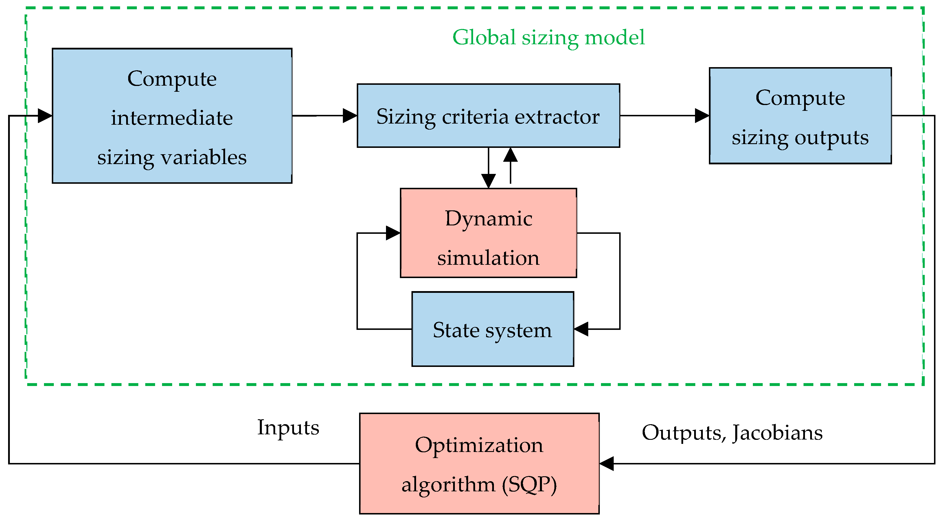
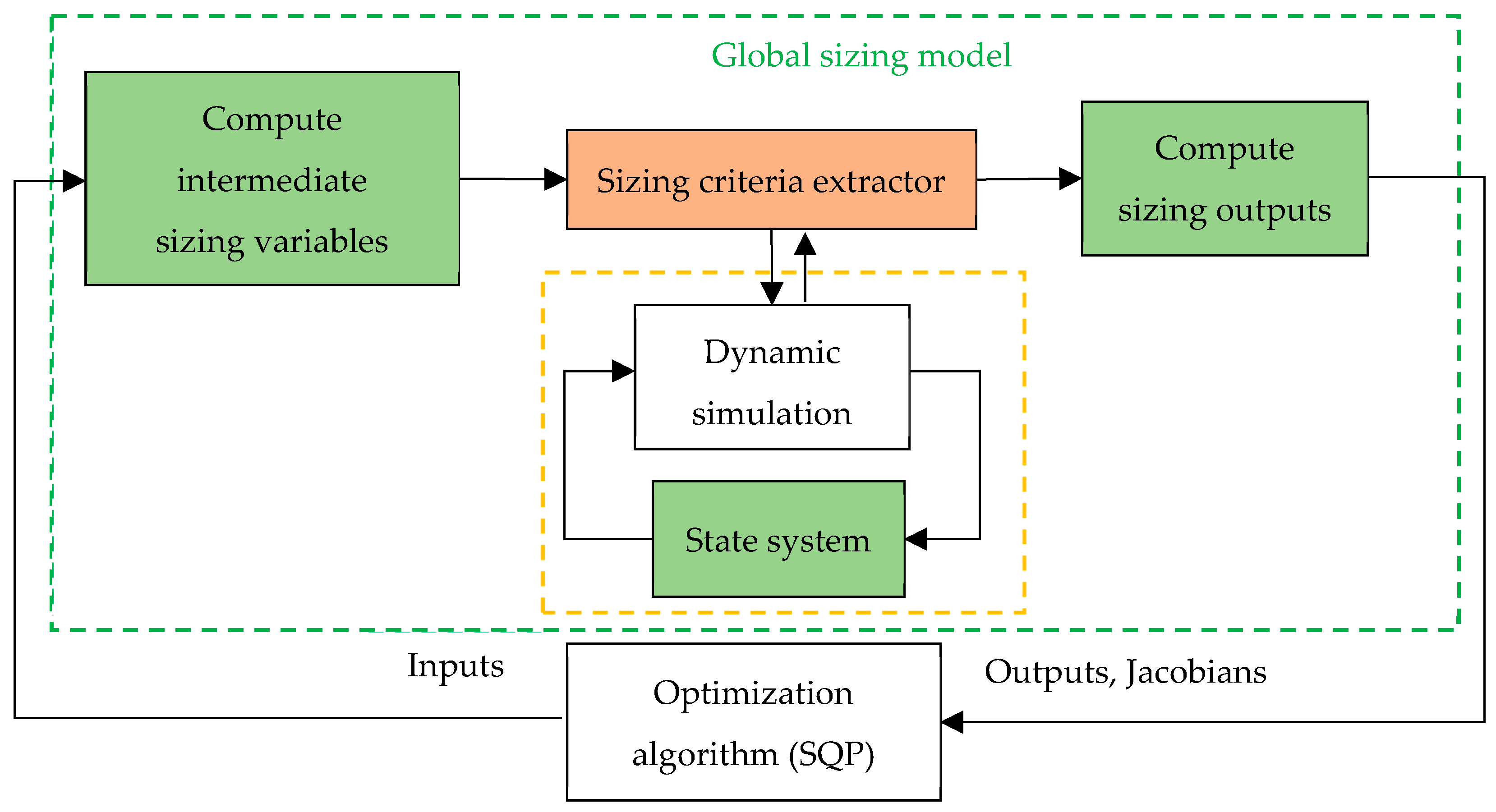
2.2. General Principle of the Methodology

This paper advocates for the utilization of an AD in regard to the optimization of dynamic systems governed by hybrid ODEs. Within the optimization loop, a time-domain simulation of a system with changing configurations is executed without retaining the values until a steady state is attained (the details of this process will be elaborated in this section). Subsequently, the simulation is conducted over a single operating period to compute various sizing criteria (such as average values, FFT, etc.) for certain variables before concluding the simulation, thereby avoiding unnecessary computations. From this, both the time-domain and frequency-domain characteristics of the simulated variables can be extracted for constraining purposes. The overarching sizing model as part of the optimization process is illustrated in Figure 3.

The optimization process is anchored in Sequential Quadratic Programming (SQP) [17], intricately linked to the sizing model, which encompasses the following components:

• An ODE system, along with tests designed to detect their variations, enabling the computation of time derivatives of state variables and beyond;
• A time-domain simulator that adeptly resolves problems in regard to ODE systems, yielding the values of state variables throughout the simulation, without necessitating post-processing of the sizing data;
• A criterion for halting the time-domain simulation, which involves the computation of sizing criteria subsequent to the detection of the steady-state conditions;
• An extractor of the sizing criteria that provides both time-domain and frequency-domain features, derived from an FFT computation, and that serve as constraints within the optimization problem;
• The gradient-based optimization algorithm SQP, which adeptly addresses the complexities of nonlinear constrained optimization.

A robust interconnection between the computation of the sizing criteria and the dynamic process has been deliberately established, thereby obviating the need for state vector storage and facilitating the implementation of advanced control strategies, such as the stopping criteria delineated in this paper.

In the subsequent subsections, we shall elaborate on the various facets of the methodology, including the selection of derivation techniques, the “white-box” hybrid ODE solver, the identification of events that necessitate alterations in the configurations of dynamic systems, the detection of steady-state conditions, and the extraction of the sizing criteria.

2.3. Derivation Techniques Used

2.3.1. Choice of Derivation Techniques

A pivotal aspect of the methodology involves the precise calculation of gradients for each segment of the simulation process and the modeling elements previously described. Diverse derivation techniques are employed, tailored to each component of the optimization process. This paper aspires to utilize the most efficient technique pertinent to each modeling aspect, as follows:

• For mathematical expressions that vary from one dynamic model to another (e.g., the dynamic model), automatic differentiation (AD) is employed to facilitate user implementation;
• For mathematical expressions that maintain a generic nature across different models (e.g., the computation of sizing criteria), symbolic derivation is utilized to streamline the computational graph of AD [18];
• For the amalgamation of derived numerical methods and mathematical expressions that are generic across different models (e.g., the hybrid ODE solver), a synthesis of AD and symbolic derivation is adopted.

The derivation techniques employed for each segment of the modeling process are succinctly summarized in Figure 4.

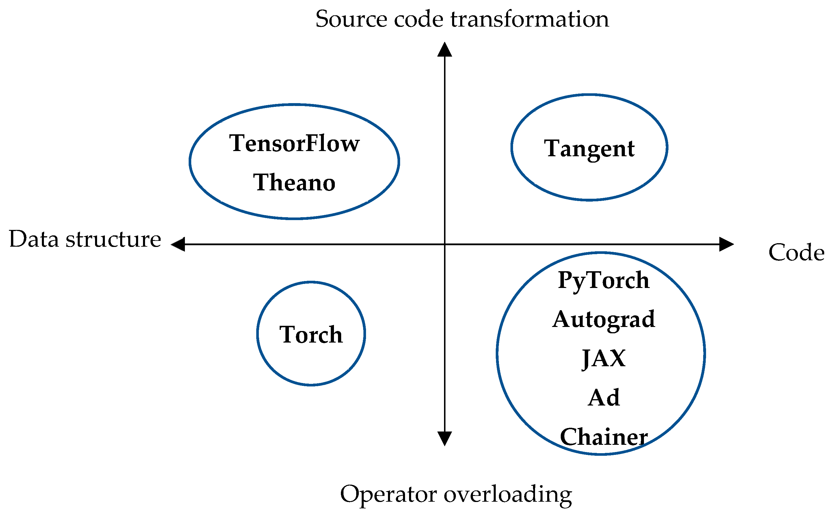
2.3.2. Automatic Differentiation (AD)

Automatic differentiation (AD) meticulously computes the precise derivatives of a computer program for a specified set of arguments [19,20,21]. This technique can be realized through the use of two distinct methodologies, as follows:

• The transformation of source code, which generates a tailored code for the function to be differentiated;
• Operator overloading, which facilitates the real-time computation of derivatives through operations defined within programmed classes.

In certain instances, the structures of computer programs may not always be correctly differentiated by AD (e.g., tests concerning ‘if’ conditional statements) without the use of specific assumptions. This represents the primary limitation of the technique, although it still offers a valuable trade-off in regard to differentiating computer code [19,20,21].

2.4. Principe of the Hybrid ODE Solver

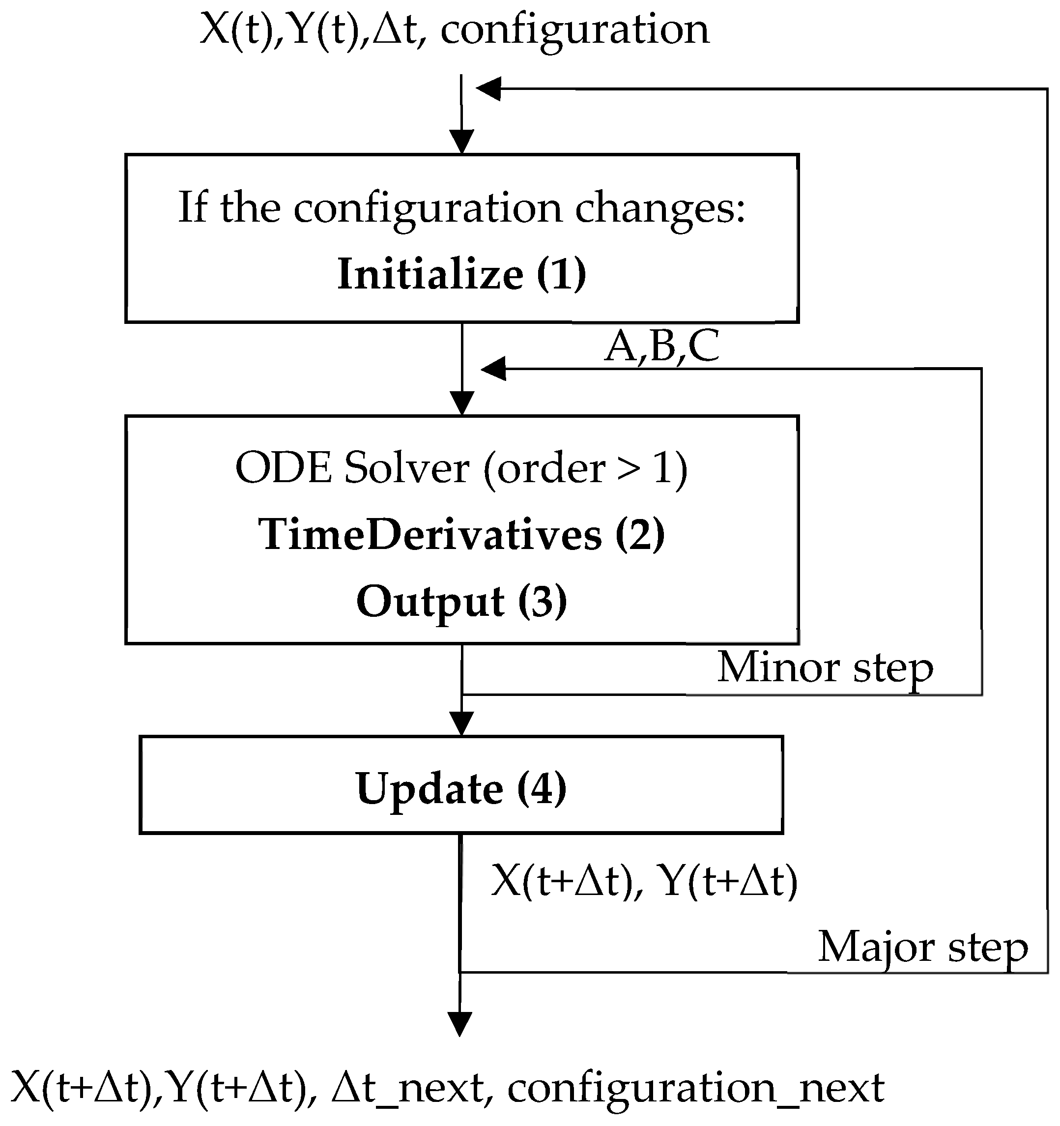
2.4.1. Resolution Scheme with S-Function Norm

In this paper, state-space representations, as presented in system (1), are considered. The model is composed of a first-order ODE and output vector expression, obtained using the computed state vector. The initial conditions are assumed to be equal to zero.

$$\left\{\begin{array}{c}{\displaystyle \frac{\mathrm{d}\mathrm{X}}{\mathrm{d}\mathrm{t}}}=\mathrm{f}\left(\mathrm{X},\mathrm{t},\mathrm{I}\right)\\ \mathrm{Y}=\mathrm{g}(\mathrm{X},\mathrm{t},\mathrm{I})\end{array}\right.$$

(1)

Here:

• X is the state vector of length n_x, according to the state representation;
• Y is the time output vector of length n_y, according to the state representation;
• t is the simulation time;
• I is the sizing input vector of length n_I;
• f and g are the vector and C² class function.

The dynamic simulation process is illustrated in Figure 5.

The user engaging with this methodology is required to delineate the generic functions, highlighted in bold in Figure 5. These functions are inspired by the FMI standard [22] and the S-function utilized in Matlab/Simulink [23,24], as follows:

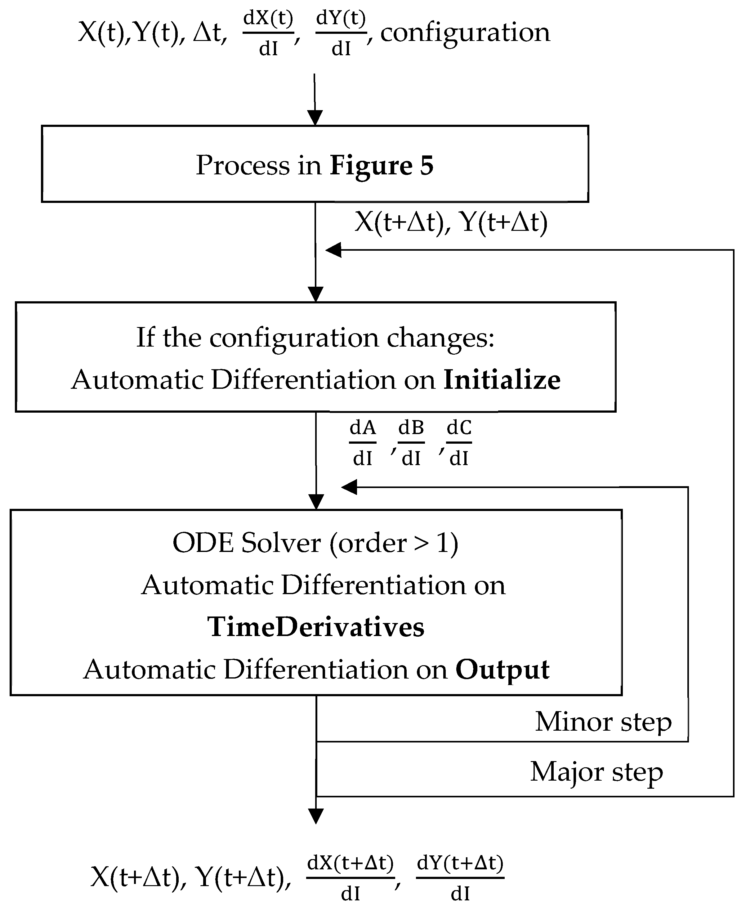
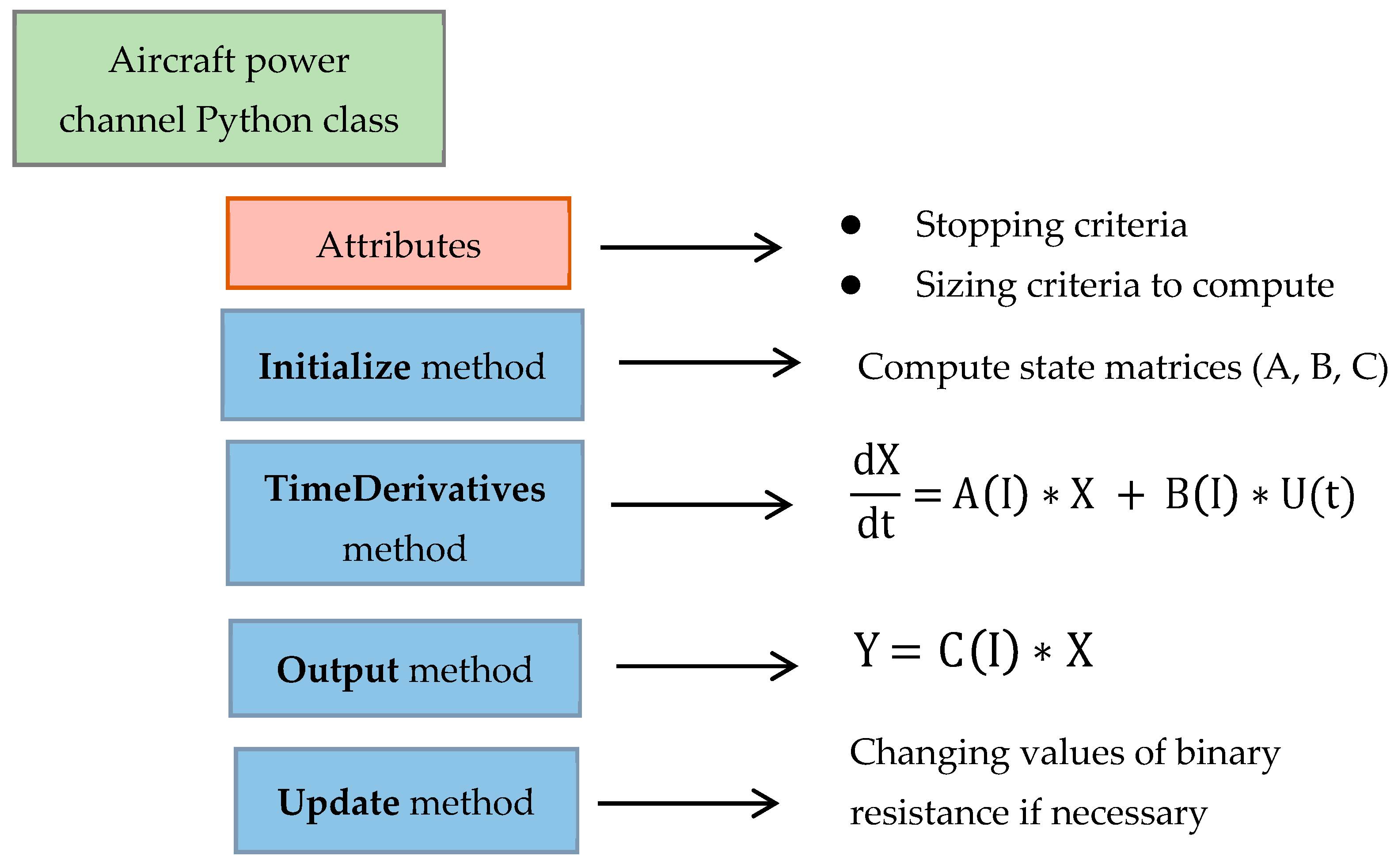
• Initialize (block (1) in Figure 5) provides the state matrices A, B, and C (refer to Appendix A), which are employed to compute the state and output vectors, but only if the circuit configuration has been altered since the previous iteration;
• TimeDerivatives (block (2) in Figure 5) yields the time derivatives of the state vector, which are invoked during each minor step in the Runge–Kutta process [25]. Following this, the optimal time step for the subsequent iteration of the process is ascertained;
• Output (block (3) in Figure 5) generates the time output vector;
• Update (block (4) in Figure 5) encompasses the necessary tests to modify the variable resistance (representing the switches) values in response to their state.

2.4.2. Gradients of the Hybrid ODE Solver

Directly applying AD to an algorithm, such as the ODE solver, may result in a sluggish performance, particularly when the algorithm is laden with numerous control flow structures [20]. Furthermore, the AD tool extracts all the input parameters from the program code, regardless of whether they are numerical, which can ultimately lead to precision challenges. As referenced in [26,27], this is not the ODE solver that has be derived, but the state-space representation, as illustrated in system (2). The novelty of this paper is the use of AD to evaluate the right-hand side of both the ODE system derived and the output expressions in (2). This is feasible due to the continuity properties inherent in the employed ODEs.

$$\left\{\begin{array}{c}{\displaystyle \frac{\mathrm{d}}{\mathrm{d}\mathrm{t}}}\left({\displaystyle \frac{\mathrm{d}\mathrm{X}}{\mathrm{d}\mathrm{I}}}\right)={\displaystyle \frac{\mathrm{d}\mathrm{f}\left(\mathrm{X},\mathrm{t},\mathrm{I}\right)}{\mathrm{d}\mathrm{I}}}\\ {\displaystyle \frac{\mathrm{d}\mathrm{Y}}{\mathrm{d}\mathrm{I}}}={\displaystyle \frac{\mathrm{d}\mathrm{g}(\mathrm{X},\mathrm{t},\mathrm{I})}{\mathrm{d}\mathrm{I}}}\end{array}\right.$$

(2)

The segment concerning the gradient computation within the dynamic simulation process is illustrated in Figure 6.

It is essential to note that discontinuities arise solely at ODE transitions, triggered by unpredictable events, while the system remains continuous with each configuration. As will be detailed in Section 2.5, unpredictable events are meticulously managed, ensuring that no complications occur when differentiating the ODE system. In fact, only the state system is differentiated, not the transitions.

2.5. Events Management

2.5.1. The Need for an Adaptive Step Size

To effectively simulate the dynamic model, the inclusion of an adaptive step size is imperative for several reasons, as follows:

• As elucidated in the subsequent subsection, certain events transpire during the simulation that necessitate detection in order to modify the model’s configuration. Occasionally, it becomes essential to recompute a simulation point at a prior moment during the simulation. Should a fixed step size be employed for efficiency, it must be exceedingly small, thereby prolonging the computation time of the simulation. Hence, an adaptive time step is favored in this context;
• The simulation must be halted once the sizing criteria have been established. Initially, the steady state of the model must be identified. Subsequently, another operating period must be conducted in a steady state to ascertain the sizing criteria;
• The FFT computation, detailed in the following subsection, necessitates a time-domain simulation recorded at fixed sampling intervals. Consequently, the adaptive time step will be adjusted to capture simulation points that adhere to the sampling period.

2.5.2. Event Detection to Change the Configurations

In this context, power electronics applications are characterized by an ODE whose parameters fluctuate throughout time-domain simulations, contingent upon the values of the state variables or observable variables. The ODE solver must identify these changes, typically by conducting tests on the simulated variables. Such tests are referred to as events (for instance, zero crossings in Matlab/Simulink). These events can be managed through the use of the “correction” method [28], as demonstrated in [16]. It is noteworthy that correction methods (not necessarily applicable in this case) are implemented in numerous power electronics solvers, utilizing an adaptive time step.

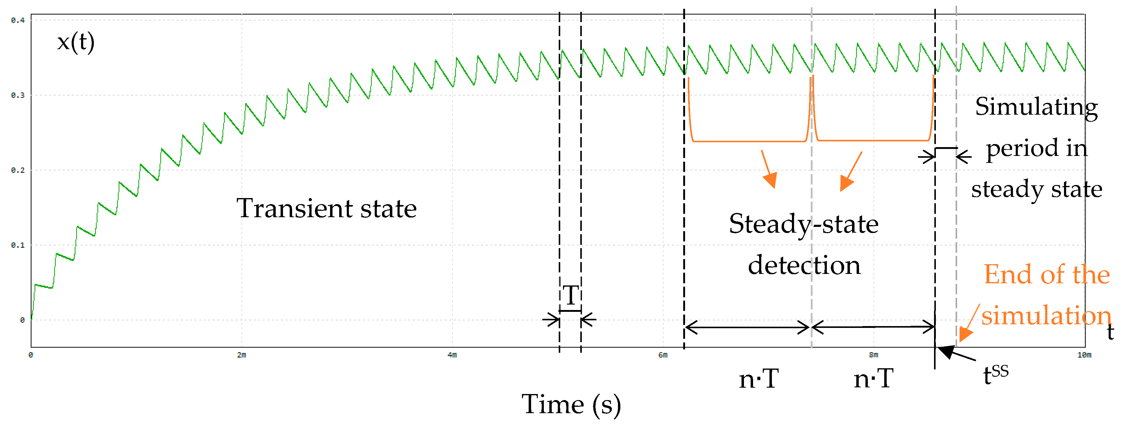
2.5.3. Stopping Criteria: Steady-State Detection

In regard to optimization problems involving electrical systems, frequency-domain constraints are computed during the steady state. To conserve computation time, it is crucial to attain a steady state before carrying out the simulation for one operating period, prior to halting the simulation [29]. In this scenario, the transient state need not be recorded, as the features are computed following the detection of the steady state. However, after identifying the steady state, another period of simulation must occur and the data may be stored for potential post-processing (if required). The process of detecting the steady state of a system is elaborated in [16], and illustrated in Figure 7.

In Figure 7:

• T is the operating period;
• n is the number of operating periods chosen to detect the steady state;
• t^ss is the time wherein the steady state is detected.

2.6. Extraction of Sizing Criteria

The sizing criteria have to be extracted from the dynamic simulation process. This aspect has already been detailed in [16,30,31]. In this subsection, precision values are added only to the criteria used in Section 4, such as the extrema values (time-domain features) and the magnitude of the frequency spectrum (frequency-domain features).

2.6.1. Time-Domain Features

Extrema Values

For each iteration of the simulation, the value of a state variable at a given time is compared to its preceding values; if it is smaller (or larger, in the case of the maxima) than the previous value, it supplants the latter as the new minimum (or maximum) value.

2.6.2. Frequency-Domain Features

As the computation of each state or output variable’s FFT has already been developed in [16,31], a special focus is placed on the spectrum magnitude, derived from the FFT. The result of the FFT is a frequency vector composed of complex numbers, from which the spectrum magnitude is derived, as indicated by expression (3).

$$\forall \mathrm{k}\in \left[0,\mathrm{M}-1\right],\left|\widehat{\mathrm{x}}\left(\mathrm{k}\right)\right|=\sqrt{\mathrm{R}\mathrm{e}{\left(\widehat{\mathrm{x}}\left(\mathrm{k}\right)\right)}^2+\mathrm{I}\mathrm{m}{\left(\widehat{\mathrm{x}}\left(\mathrm{k}\right)\right)}^2}$$

(3)

Here:

• x is a component of X, and $\widehat{x}$ its FFT;
• M is the number of points in the frequency spectrum.

Each element of the FFT vector corresponds to a frequency. The first element represents the average value (its frequency being zero), the second corresponds to the fundamental frequency f_found, while the remaining elements pertain to the harmonics. Subsequently, the requisite elements for optimization are extracted.

The derivatives of the FFT module are computed using the analytical formula provided in expression (4).

$$\begin{gathered} \forall \mathrm{i}\in \left\{1,\dots ,\mathrm{n}\mathrm{I}\right\},\forall \mathrm{k}\in \left[0,\mathrm{M}-1\right], \\ {\displaystyle \frac{\partial \left|\widehat{\mathrm{x}}\right|}{\partial {\mathrm{I}}_{\mathrm{i}}}}\left(\mathrm{k}\right)={\displaystyle \frac{\mathrm{R}\mathrm{e}\left(\frac{\partial \widehat{\mathrm{x}}}{\partial {\mathrm{I}}_{\mathrm{i}}}\left(\mathrm{k}\right)\right)·\mathrm{R}\mathrm{e}\left(\widehat{\mathrm{x}}\left(\mathrm{k}\right)\right)+\mathrm{I}\mathrm{m}\left(\frac{\partial \widehat{\mathrm{x}}}{\partial {\mathrm{I}}_{\mathrm{i}}}\left(\mathrm{k}\right)\right)·\mathrm{I}\mathrm{m}\left(\widehat{\mathrm{x}}\left(\mathrm{k}\right)\right)}{\sqrt{\mathrm{R}\mathrm{e}{\left(\widehat{\mathrm{x}}\left(\mathrm{k}\right)\right)}^2+\mathrm{I}\mathrm{m}{\left(\widehat{\mathrm{x}}\left(\mathrm{k}\right)\right)}^2}}} \end{gathered}$$

(4)

Here:

• I_i is a component of I.

Remark: The FFT can also be implemented similarly to average or RMS values. Here, the authors aim to illustrate the post-processing extraction of a sizing criteria computation.

Alternative methods for computing the FFT are detailed in [32], yet the authors sought a rapid and straightforward approach to computing the frequency-domain features.

In this section, we have meticulously detailed the methodology. We shall now proceed to elucidate its implementation within an open-source software framework.

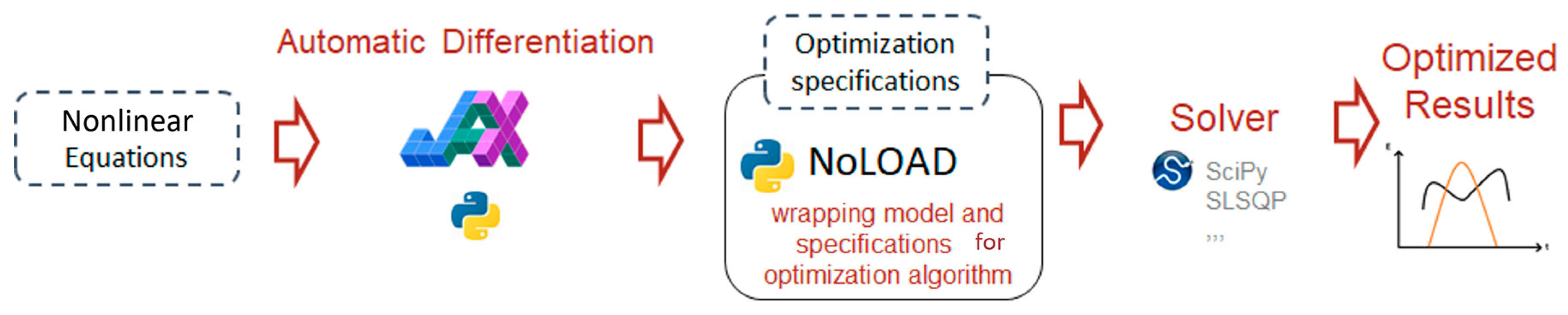
3. Implementation of the Methodology Using the NoLOAD Software

3.1. NoLOAD Software

The methodology has been seamlessly integrated into the open-source Python software, known as NoLOAD, as referenced in [33]. To ensure a high degree of coupling and enhanced performance, the various generic components of the methodology have been articulated in the same programming language, Python. The resolution of the ODE system has been accomplished through the implementation of the Runge–Kutta 5 (7M) method, utilizing Dormand–Prince coefficients [27,34]. The structure of NoLOAD is summarized in Figure 8.

3.2. Choice of the Solver

The Runge–Kutta 45 solver was used in the methodology for several reasons, as follows:

• It is widely used in electrical drive problems (containing power electronics models), and is supported by numerous software tools, such as Matlab/Simulink (https://fr.mathworks.com/products/matlab.html);
• Its adaptable variable step size makes it particularly suitable for discrete events and Fast Fourier Transform (FFT) computations.

As a result, there is no necessity for a ‘stiff’ solver, since the step size is significantly reduced for each switch’s commutation, thereby preventing numerical issues and managing the apparition of a faster or slower dynamic. After a commutation, even if the time step is strongly reduced, it increases rapidly in order to adapt to the simulated dynamic if the dynamic is slow.

Furthermore, the solver needed to be stopped automatically once the sizing criteria were computed, specifically, after detecting the steady-state conditions and completing one full operating period, which is not a feature of most contemporary solvers.

Finally, one of the key constraints during the programming phase was the need for access to the solver’s source code, allowing us to integrate it with the model. Consequently, a compromise was found between computational performance and the advantage of having a “white-box” solver.

The aim of this paper is not to compare the performance of the selected ODE solver with others, but rather to examine the efficacy of the various optimization approaches. This will be addressed in Section 4.

3.3. Variable Selectivity: Improvement Compared to CADES

One of the notable advancements of NoLOAD over the CADES software employed in G2Elab [35] lies in the selective approach it adopts for choosing the variables to differentiate. Since NoLOAD is implemented in Python, a scripting language that offers greater user intuitiveness and does not enforce variable typing, it dynamically assesses whether a variable warrants differentiation. In this context, the specifications allow for the implicit designation of the sizing outputs to be differentiated with respect to the sizing inputs. Consequently, unlike CADES [35], the size of the Jacobian matrix is markedly reduced, leading to a significant enhancement in computational efficiency.

3.4. The Automatic Differentiation Library, JAX

As previously introduced in Section 2.3.1, AD is a technique that has been in existence for several decades [36]. Over the past ten years, a plethora of AD libraries has emerged, designed for applications involving machine learning and Artificial Intelligence. A selection of these libraries is categorized according to their implementation techniques [37,38,39,40,41,42,43,44,45], as illustrated in Figure 9:

AD possesses the remarkable ability to derive control flows, encompassing constructs such as ‘while’ and ‘for’ loops, as well as ‘if’ conditional statements. This capability proves invaluable for a multitude of physical modeling applications, particularly in the realm of power electronics.

In regard to the methodology proposed herein, the Python library, JAX [46], is employed, renowned for its Just-In-Time (JIT) compilation feature, which significantly accelerates code execution. This efficiency is particularly advantageous given the extensive simulations required in regard to optimization problems. Furthermore, JAX empowers programmers to define their own ‘derivative’ versions of Python algorithms when alternative methods for derivative computation are available. It facilitates the invocation of user-defined external functions, enabling the calculation of both their outputs and gradients. Notably, these functions may be implemented in languages other than Python, such as C, C++, or Java, a feature that has been validated within the NoLOAD framework.

3.5. Parts of the Methodology to Be Implemented by the Designer

The methodology delineated in this paper is seamlessly integrated into the NoLOAD software, thereby relieving designers of the need to redevelop it. As illustrated in Figure 3, this encompasses the ODE solver, the identification of the system’s steady state, the computation of the FFT, the extraction of features in regard to both time and frequency domains, and the application of AD to ascertain the model’s gradients.

Designers are tasked with defining their models within a particular class, specifically outlining the generic methods depicted in Figure 5, which include Initialize, TimeDerivatives, Output, and Update. Additionally, they must specify in regard to the solver which time or frequency features are to be extracted from the simulation for the optimization task.

With the implementation of the methodology within the open-source software now established, it is poised to be applied to the optimal design of the aircraft power channel application.

4. Application to Power Electronics

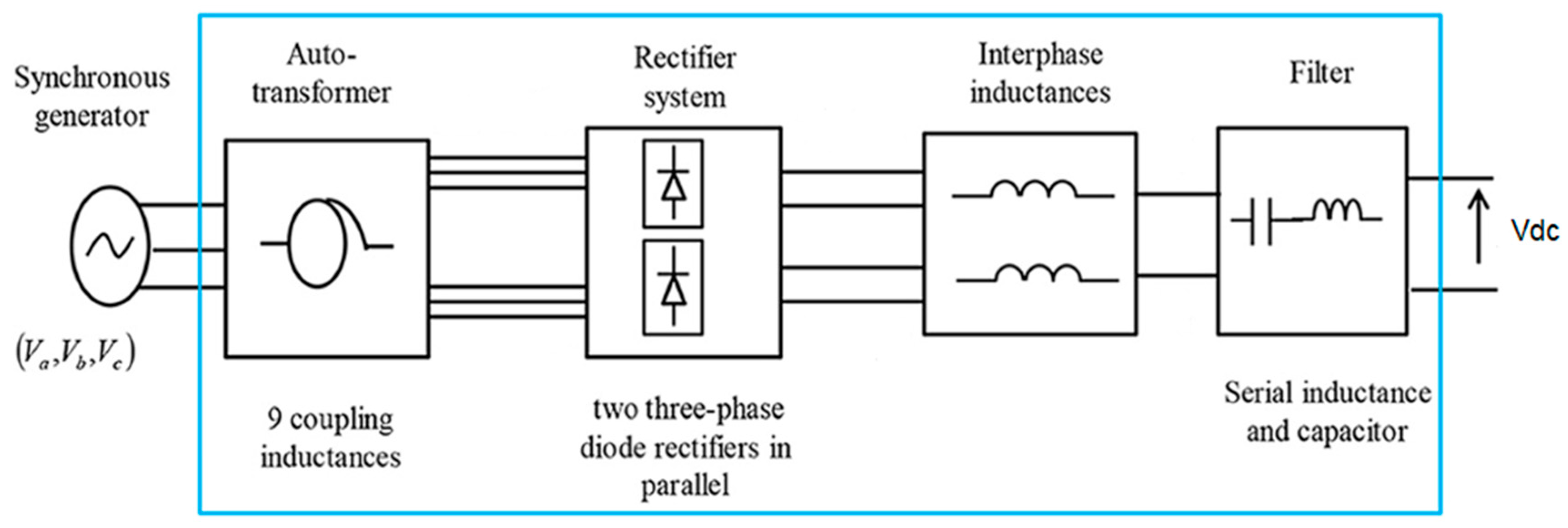
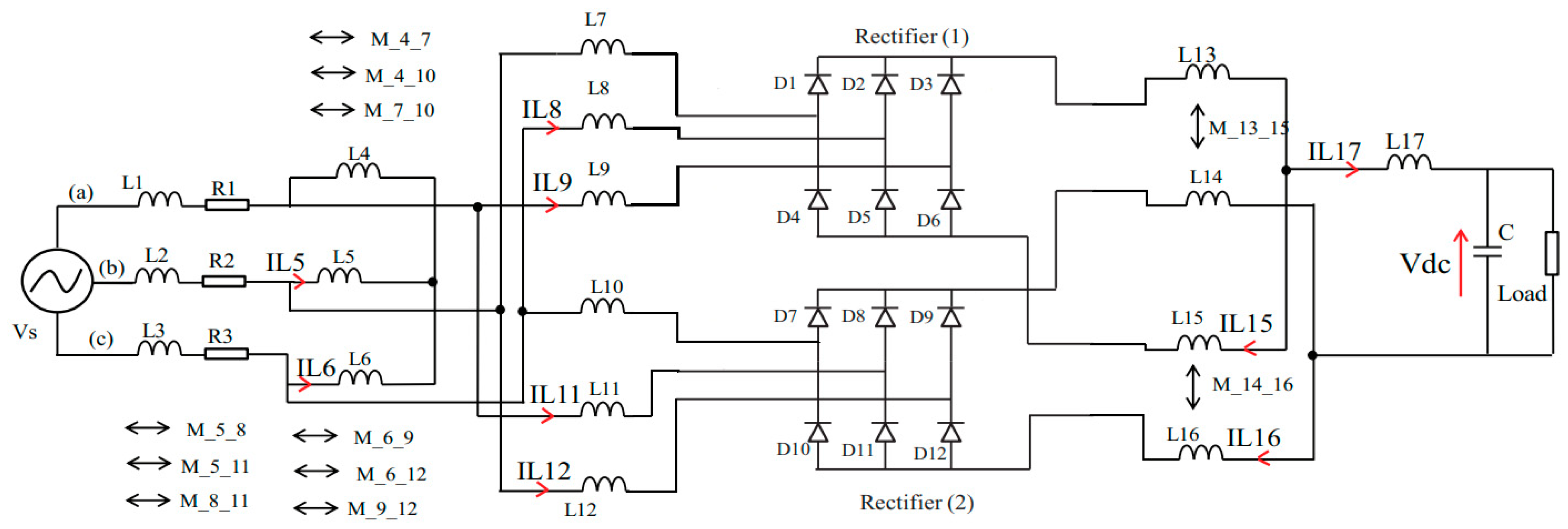
4.1. Presentation of the Application

This paper illustrates the proposed approach with the sizing of an aeronautic power channel presented in Figure 10. It is composed of an autotransformer, a rectifier system defined by two three-phase diode rectifiers in parallel, two interphase inductances, and a harmonic filter.

In Figure 10:

• (Va, Vb, Vc) = Vs is an AC three-phase voltage source;
• Vdc is the channel output voltage.

The electrical system for this application is presented Figure 11.

In Figure 11:

• (a,b,c) corresponds to each of the three-phase of the voltage source.
• f is the frequency of Vs;
• Vdc, iL5, iL6, iL8, iL9, iL11, iL12, iL15, iL16, iL17 are state variables;
• Currents and voltages of diodes D1 to D12 are state outputs, such as the channel input currents iL2, iL3.

Given that the application operates solely through natural switching, its behavior remains inherently unpredictable, thereby complicating the modeling and optimization processes necessary for effective sizing. Consequently, the analytical model of the application cannot be established without any a priori on the model. The sizing was approached using various methodologies outlined in [11], specifically by addressing a mono-objective optimization problem, as follows:

• A time-domain simulator (Saber) was employed, in conjunction with a stochastic particle swarm optimization (PSO) algorithm, successfully resolving the optimization challenge within a time span of 2 days for a single run;
• SQP was utilized, alongside a finite difference method, to compute the gradients. An analytical model was crafted to ascertain the frequency-domain characteristics, albeit with a priori knowledge regarding operational modes. This necessitated that the sizing was conducted based on these modes, consequently narrowing the solution space. This optimization problem was also resolved in 2 h for one run.

For the determination of capacitances and inductances, analytical models were developed as described in [11], leveraging the geometrical parameters of the aircraft’s power channel components. However, these models are not detailed within this paper, which primarily focuses on the dynamic model and the time-domain simulations. It is worth noting that the component models have been thoroughly validated, as demonstrated in [47], with simulation models being benchmarked against established reference simulators, such as Saber [47].

4.2. Specifications in Terms of the Optimization Problem

4.2.1. Optimization Inputs

The optimization inputs in terms of the problem are summarized in

Table 1. Inputs in regard to the optimization problem.

Name of the Optimization Input and Description	Bounds
	Min	Max
a1: Coefficient in regard to primary and first secondary coupling matrices	0.01	2.1706
a2: Coefficient in regard to primary and second secondary coupling matrices	0.01	2.1706
kd: Ratio between the winding width and the magnetic core width of the autotransformer	0.032	3.63
np: Number of primary turns for the autotransformer	10	45
kdi: Ratio between the winding width and the magnetic core width of the interphase inductance	0.02	9
ni: Number of primary turns for each interphase inductance	7	203
L17: Filter inductance	10−6	10−4
C: Filter capacitance	6 × 10−6	10−3
kdf: Ratio between the winding width and the magnetic core width of the filter inductance	0.0013	52
nf: Number of filter inductance turns	1	30

. They deal with the geometrical or physical aspects, to allow us to compute most of the inductance-related geometrical parameters and the resistance detailed in Figure 11, excluding R1, R2, R3, L1, L2, and L3, and the ‘Load’ resistor, which are fixed parameters.

4.2.2. Optimization Constraints

The aim of the optimization endeavor is to minimize the mass of the aircraft’s electrical power channel. This intricate optimization problem is governed by several constraints, as follows:

• Geometric constraint: the Routh Criterion, which must remain positive. To compute this value, a global equivalent circuit of the aircraft power channel was established, based on an RL series circuit [11]. It was achieved by bringing all the resistance and inductance components to the continuous side. Therefore, the Routh Criterion is applied in this linear continuous system, which represents the global behavior of the system;
• Frequency-domain constraints: The input current (iL2) of the channel must adhere to the standards delineated in

  Table 2. Frequency-domain constraints for IHR ($\widetilde{\mathrm{i}\mathrm{L}2}$).

  Harmonic Order (k)	Upper Bound (in %)
  k = 3	IHRk < 2
  k = 11	IHRk < 10
  k = 5, 13	IHRk < 8
  k = 17, 19	IHRk < 4
  k = 7, 23, 25	IHRk < 3
  K = 29, 31, 35, 37	IHRk < 30/k
  K = 2, 4	IHRk < 1/k
  k is a multiple of 3 or is odd	IHRk < 2
  Other cases	IHRk < 2

  , corresponding to low frequencies (up to 14,800 Hz). IHR signifies the Individual Harmonic Rate, as articulated in Equation (5) [48];
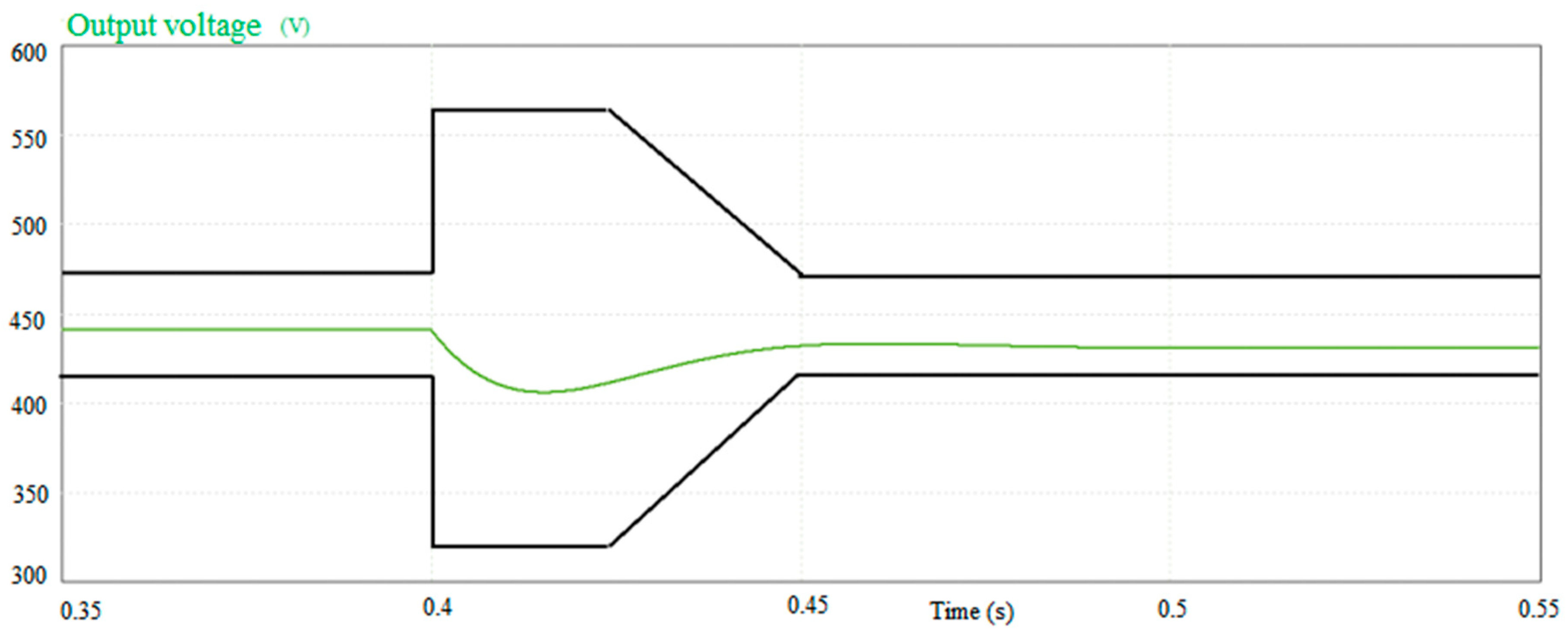
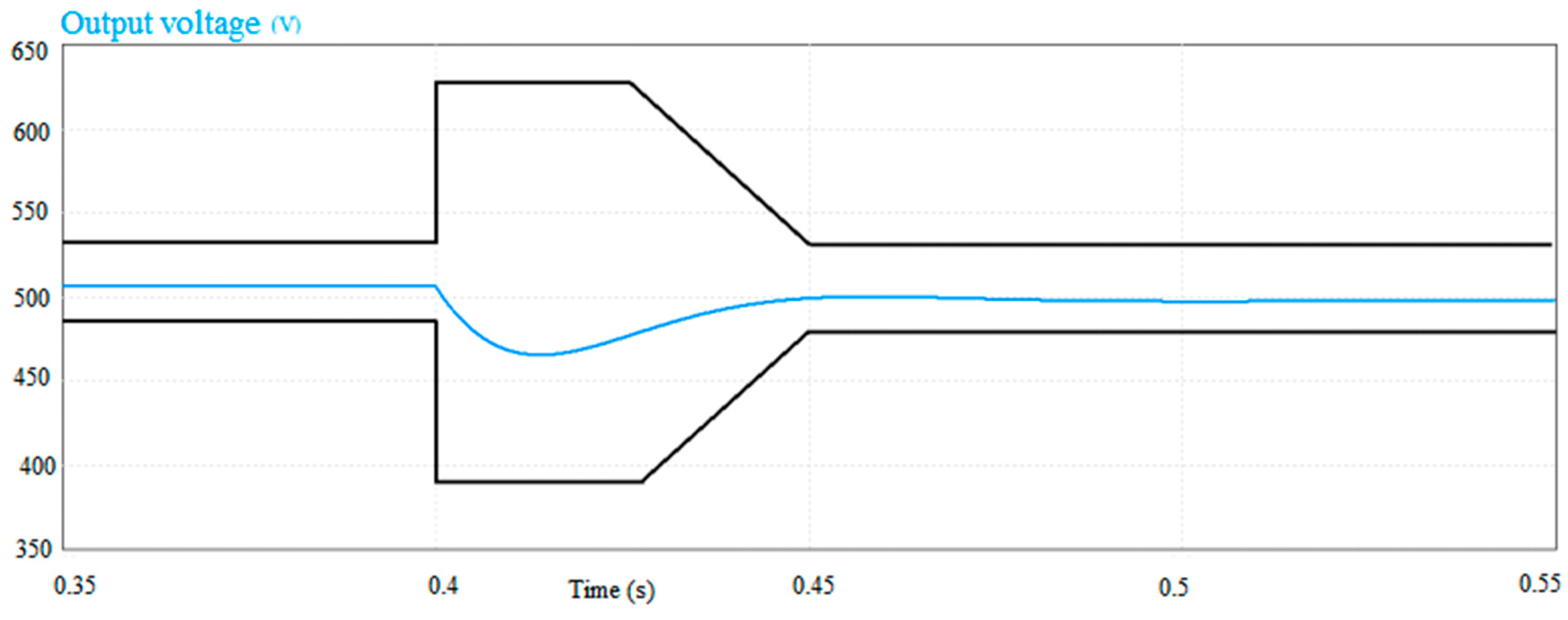
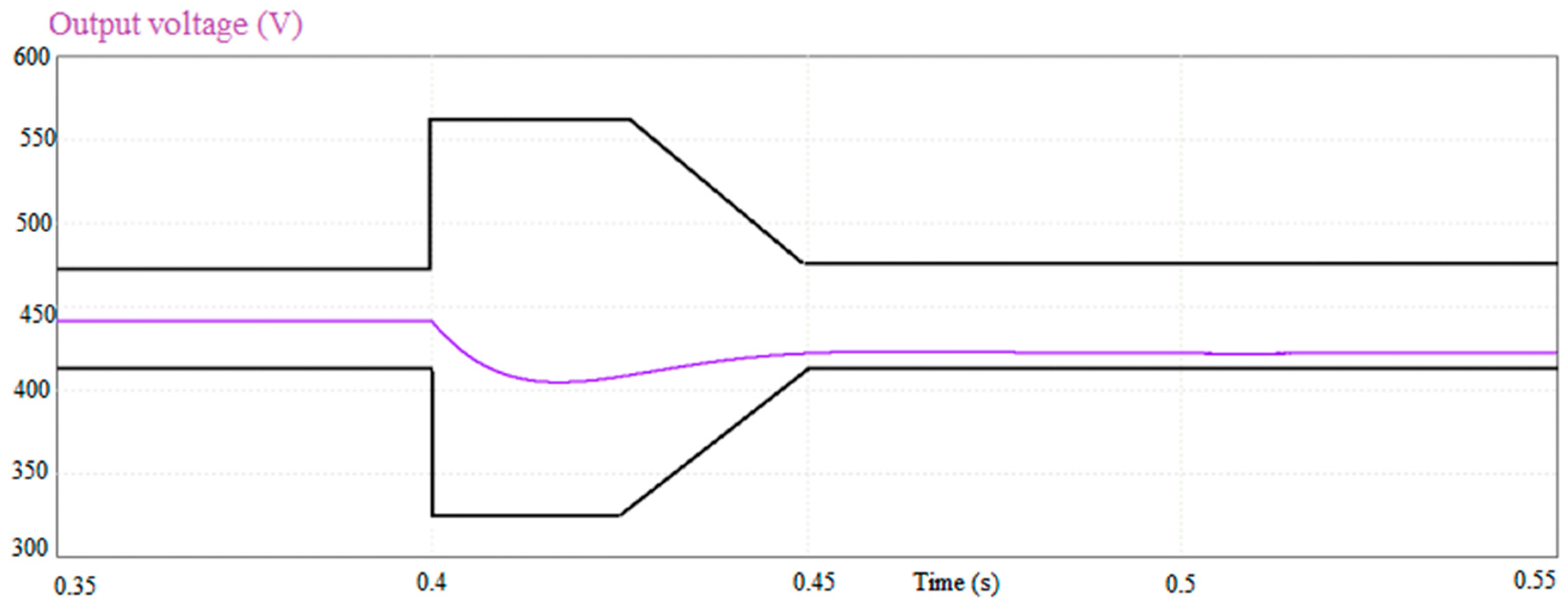
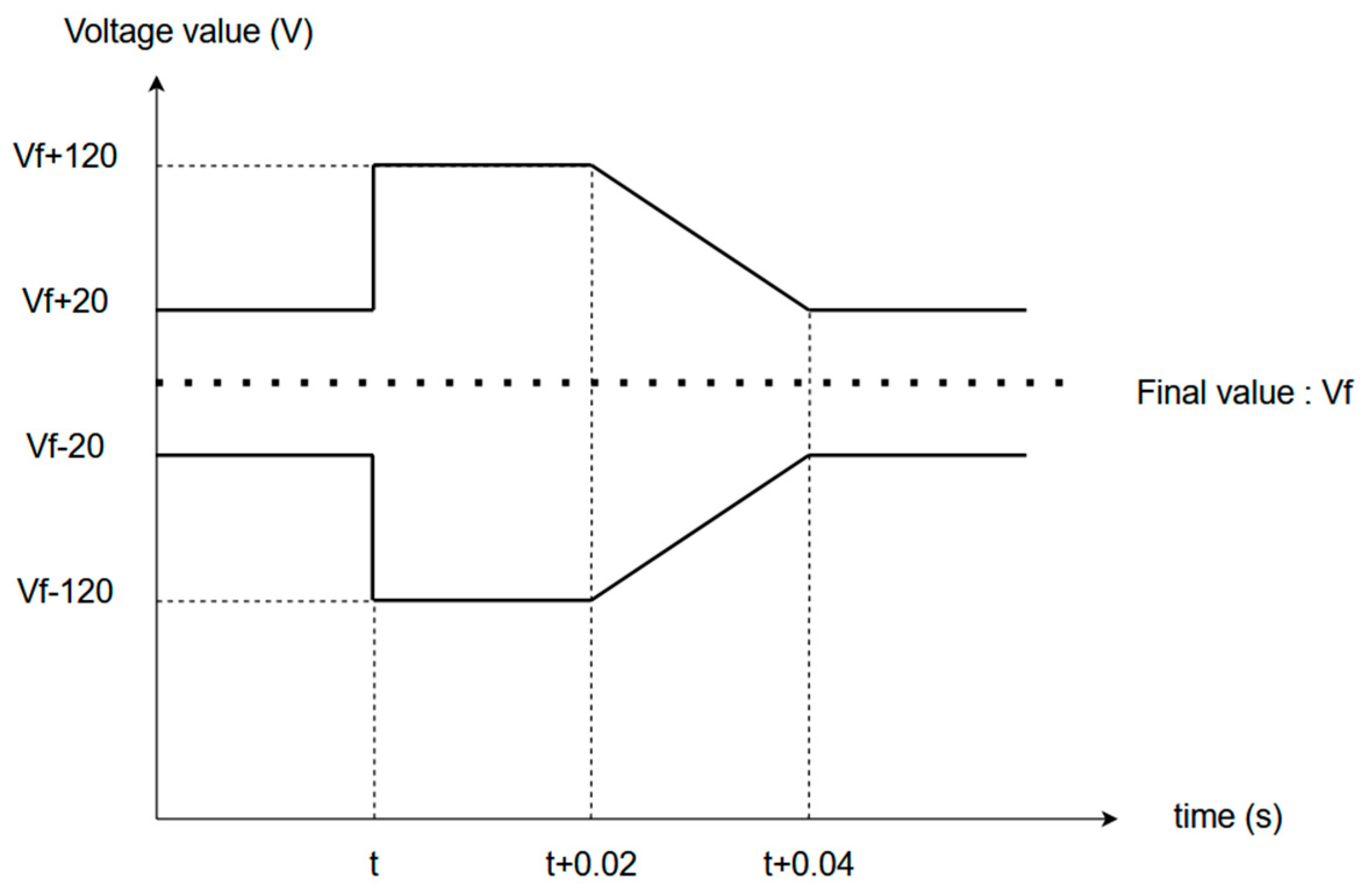
• Time-domain constraint: Upon achieving a steady state, the ‘Load’ resistance depicted in Figure 11 is diminished by one-eighth of its size to induce a disturbance and initiate a new transient state. During this transient phase, the channel’s output voltage (Vdc) must conform to the template illustrated in Figure 12. At each computational interval, should the output voltage (Vdc) deviate from the prescribed template, the constraint value is augmented by the discrepancy between the actual output and the template’s bounds. For the constraint to be satisfied, it must equate to zero. The gradients of this constraint concerning the optimization inputs are derived through automatic differentiation, as no analytical formula exists.

$${\mathrm{I}\mathrm{H}\mathrm{R}}_{\mathrm{k}}\left(\tilde{\mathrm{x}}\right)={\displaystyle \frac{\left|{\tilde{\mathrm{x}}}_{\mathrm{k}}\right|}{\left|{\tilde{\mathrm{x}}}_1\right|}}$$

(5)

Here:

• $\tilde{x}$1 is the FFT of x when the frequency is equal to the fundamental one (400 Hz);
• k is the harmonic order (from k = 2 for f = 800 Hz, to k = 37 for f = 14800 Hz).

The optimization problem encompasses 10 inputs, 1 objective function to minimize, and 38 constraints, which include the following:

• 1 equality constraint (the time-domain constraint);
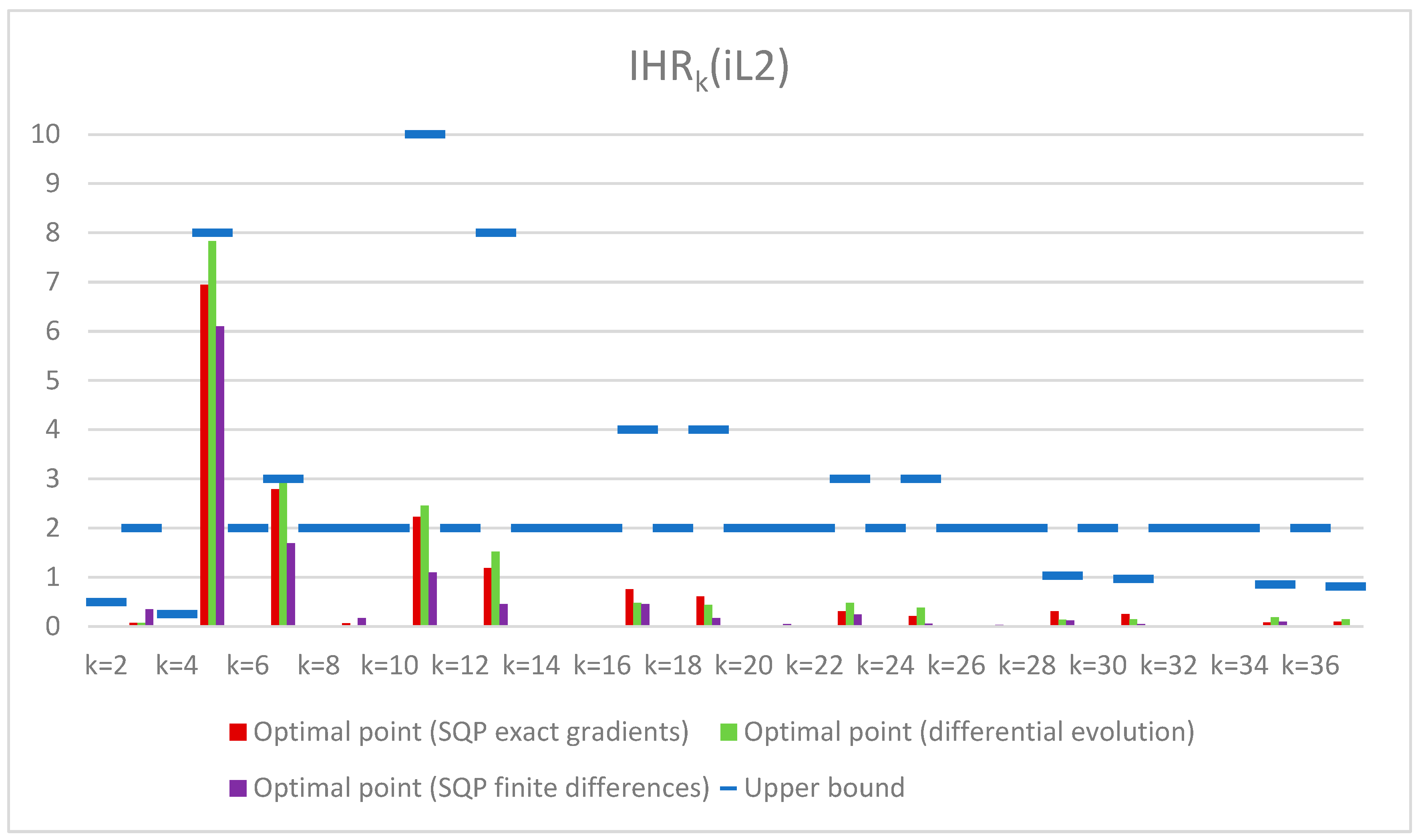
• 36 inequality constraints for the frequency-domain constraints (each corresponding performance constrained by an upper bound);
• 1 inequality constraint for the Routh Criteria, which is only constrained by a minimum value (it must be positive).

In Table 2:

• IHR ($\widetilde{iL2}$) means the Individual Harmonic Rate of the channel input current iL2.

It is noteworthy that the final value of the output channel voltage varies with each simulation, contingent upon the values of the optimization inputs.

4.3. Modelling of the Aircraft Power Channel

Each diode is characterized by a resistance that assumes a high value when activated, and a low value otherwise. The generic methods illustrated in Figure 5 are employed within this model, encompassing the TimeDerivatives, Initialize, Output, and Update methods. The incidence matrix of the electrical circuit is constructed to facilitate the computation of the state matrices (A, B, C), as delineated in Appendix A. The Initialize method executes the calculation of these state matrices, incorporating the optimization inputs. Meanwhile, the TimeDerivatives and Output methods derive the state and output vectors, utilizing the state representation articulated in Equation (6).

$$\left\{\begin{array}{c}\begin{array}{c}{\displaystyle \frac{\mathrm{d}\mathrm{X}}{\mathrm{d}\mathrm{t}}}=\mathrm{A}\left(\mathrm{I}\right)\ast \mathrm{X}+\mathrm{B}\left(\mathrm{I}\right)\ast \mathrm{U}(\mathrm{t})\\ \mathrm{Y}=\mathrm{C}\left(\mathrm{I}\right)\ast \mathrm{X}\end{array}\end{array}\right.$$

(6)

Here:

• A, B, C are state matrices depending on the optimization inputs, I;
• U is the AC three-phase voltage source vector.

The Update method delineates the events that may prompt a reconfiguration of the model; these events are inherently unpredictable, corresponding to instances when the currents through or the voltages across the diodes reach zero, effectively signifying a change in sign, and, thus, altering their states. The implementation of the aircraft power channel model within the NoLOAD environment is depicted in Figure 13.

The state representation of the aircraft electrical power channel comprises 10 state variables and 25 output variables, as detailed in Appendix A. The program code associated with the overarching sizing model encompasses the following approximate components:

• 600 lines of code, inclusive of the dynamic component’s description;
• 200 intermediate equations that model the electrical parameters derived from the geometric parameters;
• the equations governing the optimization outputs in relation to the optimization inputs (for instance, the total mass of the application and the Routh Criteria).

4.4. The Optimization Procedure

The optimization challenge is approached through the application of two distinct algorithms, as follows:

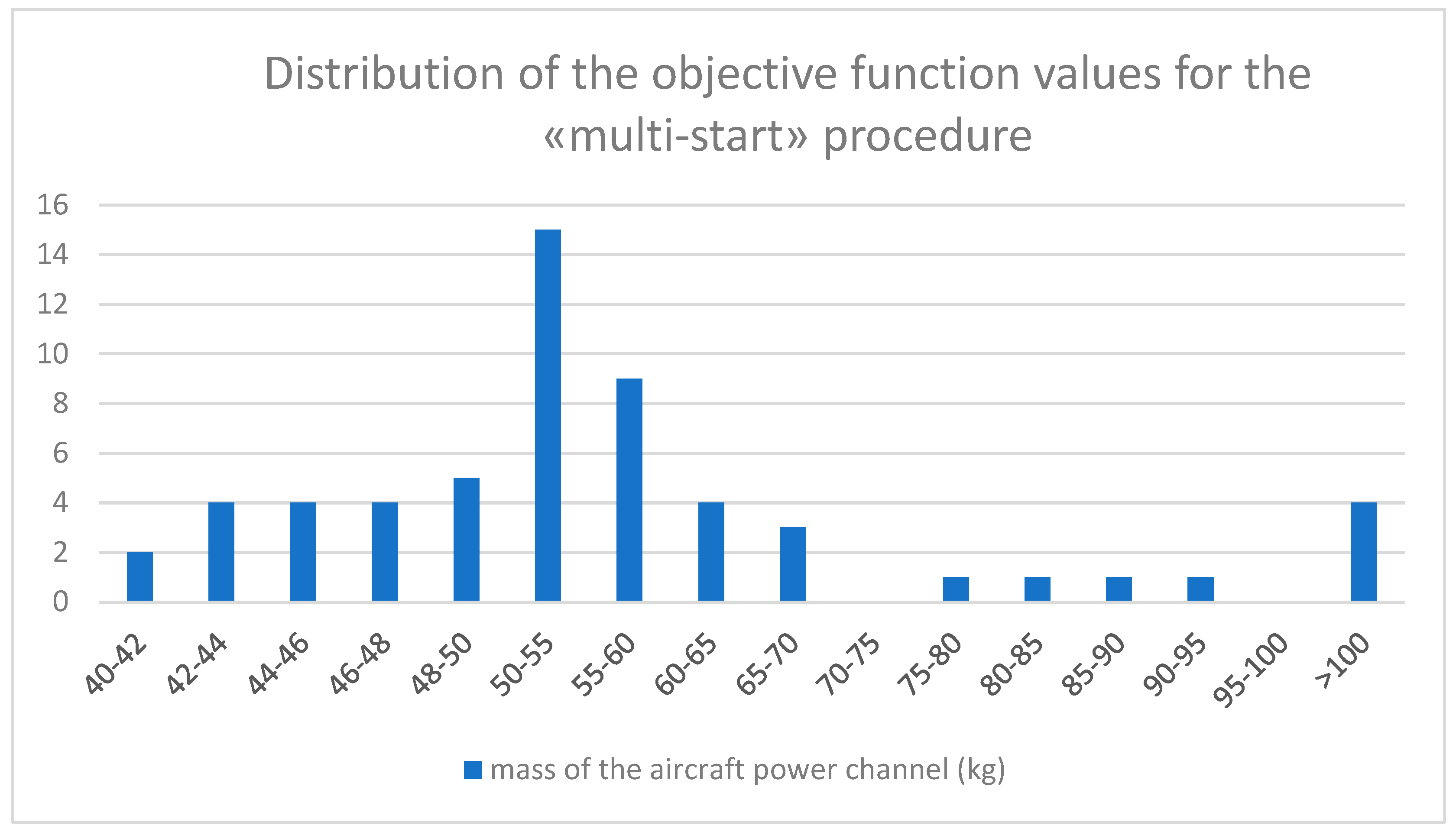
• The SQP algorithm, derived from the SciPy package, employs a «multi-start» strategy. This algorithm is executed ten times, each time initiated from randomly selected starting points, and the optimal solution that most effectively minimizes the objective function is subsequently selected. Thus, the robustness of the SQP will be improved;
• The stochastic differential evolution algorithm, also derived from the SciPy package, operates with a population of 100 individuals and is constrained in regard to a maximum of 500 generations. Given its stochastic nature, this algorithm is executed thrice to ensure that the optimal solution remains consistent across all the iterations.

To evaluate the efficacy of the gradient computation, the final outcome from the initial optimization (SQP with «multi-start») is further refined using SQP, albeit with gradients calculated via the finite difference method.

The optimization process is conducted on a computational server running Ubuntu 20.04, equipped with an Intel XEON Silver 4210R processor, featuring 10 cores (2.4 GHz) and 32 GB of RAM.

4.5. The Choice of Parameters for the Simulation

In the context of the dynamic simulation process, it is imperative to judiciously select the initial step size to prevent numerical complications during the simulation. In this instance, a notably small value, such as 10⁻⁹, is required, because the aircraft power channel has fast commutation frequencies.

Furthermore, the number of points in the frequency spectrum must be meticulously determined to ensure an accurate evaluation of the FFT, according to the Nyquist–Shannon theorem. As the last harmonic needs to occur at 15 kHz, the FFT has to be carried out based on at least 30 000 points, in order to respect the theorem. The simulation step size is automatically adapted to reach each sampling point.

4.6. Results of the Optimization Problem

4.6.1. Application Aspect

The «multi-start» procedure consists of 58 optimization runs using random initial points. The distribution of the objective function values is given in Figure 14.

The objective function values are not well-distributed because the aircraft power channel is a chaotic system in regard to its behavior.

The optimization has converged in regard to the optimum points described in

Table 3. Optimal inputs of the optimization problem for each algorithm.

Optimized Inputs	Initial Point (SQP)	Optimal Point (SQP Exact Gradients)	Optimal Point (SQP Finite Differences)	Optimal Point (Differential Evolution)
a1	0.564	0.116	0.571	0.109
a2	0.180	0.189	0.177	0.142
kd	1.88	0.526	1.84	0.584
np	14.8	37.95	15.2	41.0
kdi	2.18	0.443	2.10	0.601
ni	52.4	42.7	54.63	60.0
L17	9.67 × 10−5	6.00 × 10−5	9.69 × 10−5	10−6
C	9.69 × 10−4	8.71 × 10−4	9.68 × 10−4	5.27 × 10−5
kdf	43.1	0.917	0.700	0.971
nf	7.58	20.6	8.83	1.65

. The optimal inputs of the optimization problem for each algorithm are shown in Table 3. The outputs of the optimal solutions are presented in

Table 4. Optimal outputs of the optimization problem for each algorithm.

Optimized Outputs	Initial Point (SQP)	Optimal Point (SQP Exact Gradients)	Optimal Point (SQP Finite Differences)	Optimal Point (Differential Evolution)
Mass of the aircraft power channel (kg)	138.5	41.78	95.57	39.28
Routh Criteria	729 (>0)	1408 (>0)	975 (>0)	23 (>0)
Transient-state constraint	0 (=0)	0 (=0)	0 (=0)	0 (=0)

. The optimal outputs of the optimization problem for each algorithm are presented in Table 4. The transient-state constraint of the optimal solutions is summed up in Appendix B.

The frequency-domain constraints of the optimal solutions compared to the standard methods are presented in Figure 15 (data are listed in

Table A1. Frequency-domain constraint values for the initial points and the optimal solutions.

Harmonic Order (k)	Upper Bound (in %)	Initial Point (SQP)	Optimal Point (SQP Exact Gradients/Finite Differences)	Optimal Point (Differential Evolution)
k = 2	IHRk < 0.5	0.028	0.014/0.023	0.005
k = 3	IHRk < 2	0.62	0.075/0.35	0.077
k = 4	IHRk < 0.25	0.010	0.0014/0.011	0.0045
k = 5	IHRk < 8	0.79	6.94/6.1	7.83
k = 6	IHRk < 2	0.0057	0.0059/0.007	0.0032
k = 7	IHRk < 3	2.80	2.80/1.69	3.00
k = 8	IHRk < 2	0.0066	0.00064/0.0046	0.0015
k = 9	IHRk < 2	0.15	0.069/0.169	0.056
k = 10	IHRk < 2	0.0025	0.0029/0.0051	0.0020
k = 11	IHRk < 10	0.44	2.23/1.10	2.45
k = 12	IHRk < 2	0.0033	0.0038/0.0034	0.0026
k = 13	IHRk < 8	0.78	1.19/0.46	1.52
k = 14	IHRk < 2	0.0031	0.0011/0.0010	0.0013
k = 15	IHRk < 2	0.042	0.014/0.019	0.020
k = 16	IHRk < 2	0.0011	0.0014/0.0024	0.00039
k = 17	IHRk < 4	0.15	0.76/0.46	0.48
k = 18	IHRk < 2	0.0016	0.0020/0.0020	0.0012
k = 19	IHRk < 4	0.26	0.61/0.17	0.44
k = 20	IHRk < 2	0.0018	0.0014/0.0012	0.00044
k = 21	IHRk < 2	0.025	0.022/0.05	0.019
k = 22	IHRk < 2	0.00068	0.00015/0.002	0.00091
k = 23	IHRk < 3	0.12	0.31/0.25	0.49
k = 24	IHRk < 2	0.00070	0.0015/0.0016	0.0011
k = 25	IHRk < 3	0.12	0.21/0.061	0.38
k = 26	IHRk < 2	0.00088	0.00012/0.00039	0.00057
k = 27	IHRk < 2	0.038	0.013/0.031	0.012
k = 28	IHRk < 2	0.00031	0.0012/0.0014	0.00033
k = 29	IHRk < 1.035	0.064	0.31/0.12	0.14
k = 30	IHRk < 2	0.00051	0.0012/0.0013	0.00051
k = 31	IHRk < 0.968	0.047	0.25/0.05	0.15
k = 32	IHRk < 2	0.00019	0.00093/0.00021	0.00044
k = 33	IHRk < 2	0.038	0.0089/0.013	0.011
k = 34	IHRk < 2	0.0000683	0.00029/0.0011	0.00043
k = 35	IHRk < 0.857	0.043	0.083/0.098	0.19
k = 36	IHRk < 2	0.00077	0.00078/0.00083	0.00082
k = 37	IHRk < 0.811	0.052	0.100/0.014	0.15

of Appendix B). All the constraints are respected. For k = 5 and k = 7 frequencies, these constraints are active for the solution given by the differential evolution algorithm.

4.6.2. Computational Cost Aspect

The performance of the differential evolution and SQP algorithms are compared in

Table 5. Comparison of optimization algorithm performance.

Criteria	SQP (Exact Gradients)	SQP (Finite Differences)	Differential Evolution
Number of optimization iterations (one optimization run)	31	13	195
Number of model evaluations (one optimization run)	37	149	19,985
Number of model gradients evaluations (one optimization run)	30	13	/
Computation time (one optimization run)	6 min	1 h 13 min	2 days 20 h 57 min ≈ 70 h
Computation time (with «multi-start» procedure)	6 min × 58 = 6 h	/	70 h × 3 = 210 h

. The given performances correspond to one optimization run.

SQP demonstrates a remarkable speed advantage over differential evolution in a single optimization run, achieving a ratio of approximately 700. This underscores the significant advantages that gradients offer in the realm of optimization. Furthermore, the gradient computation technique employed in the article, a sophisticated blend of symbolic derivation and automatic differentiation, yields solutions that are not only more precise, but are also more swift than those derived through the use of the finite difference method.

In this context, the optimal solution obtained from differential evolution served as the initial point for SQP, which regarded it as an optimal solution, ultimately failing to identify a superior alternative.

The methodology articulated in reference [11], which incorporates an analytical model for frequency-domain features, alongside the SQP approach, successfully arrived at an optimal solution within a mere two hours for a single optimization run. In contrast, the innovative methodology presented in the paper resolved the optimization problem in approximately six minutes, achieving a remarkable ratio of 20 for one optimization run. This advancement signifies a notable enhancement in the optimization performance, effectively eliminating the need for a priori assumptions regarding operating modes. Additionally, the extraction of transient-state features, as introduced in this paper, represents a significant innovation, as existing methods [11] necessitate computation only after the optimization process has concluded.

5. Discussion

In this paper, we unveil a methodological framework designed to assist designers in regard to the sizing of power electronics applications. Several noteworthy aspects of this methodology merit attention, as follows:

• A specialized ‘white-box’ solver has been meticulously crafted to simulate systems governed by ordinary differential equations (ODEs), particularly those that are hybrid in nature. The expressions governing these systems are subject to change in response to unpredictable events;
• This solver possesses the remarkable ability to automatically detect when a power electronics application has attained a steady state;
• It is also equipped to extract salient features from both time-domain and frequency-domain simulations, which can subsequently be utilized as outputs for optimization;
• Furthermore, the solver is amenable to differentiation; the derivatives concerning the optimization inputs are computed through automatic differentiation for time-domain simulations, while formulas are employed for feature extraction.

The methodology has been implemented within the open-source Python library, NoLOAD [33], enabling its application to various types of power electronics systems. Notably, it has been employed for the sizing of an aircraft power channel application, demonstrating superior performance with SQP and exact gradients compared to previous methodologies [11]. Although the application discussed herein pertains to a diode-based circuit, the methodology can be extended to encompass circuits featuring active switches. Moreover, the methodology is applicable to other domains, such as mechanical engineering. In particular, economic considerations could be incorporated into the optimization problem.

In summary, this methodology enables designers to efficiently size their dynamic models, especially those composed of hybrid ODEs subject to unpredictable events, by employing gradient-based algorithms with automatic and accurate gradient computation. No a priori knowledge on the application’s operating modes is required. As a result, the resolution’s capabilities and optimization scope are significantly enhanced compared to prior work [11]. Furthermore, it represents a generic and easily implementable approach for the designer, addressing a genuine limitation in terms of the current state of the art [49,50].

6. Future Perspectives for the Methodology

Nevertheless, there remain several avenues for enhancement, as follows:

• Currently, it addresses optimization problems involving continuous variables; an extension to accommodate discrete variables is necessary;
• The paper presents a sizing approach for power electronics applications. It would be advantageous to extend this methodology to address optimization problems that encompass both sizing and optimal control, such as energy management in regard to microgrids. The integration of optimal control could be incorporated into the dynamic simulations of the proposed methodology;
• Surrogate-based algorithms yield greater precision when gradients are incorporated, thus the methodology should be employed alongside such algorithms to facilitate the sizing of larger systems characterized by state spaces with more dimensions;
• Optimization problems involving a larger number of constraints, and of greater complexity, could, in theory, be addressed using this methodology. However, the limitations regarding the computation of the Jacobian matrix (in relation to the inputs) must be clearly defined;
• The availability of gradients enables the efficient computation of global sensitivity analysis for a model using the DGSM algorithm [51];
• It would be valuable to establish a connection between this methodology and other design environments. Indeed, modeling power electronics applications remains partially manual in nature, as the designer is required to encode the model within Python script. In some instances, this process can be tedious, whereas other environments, such as Matlab/Simulink, provide a more intuitive block-based approach, facilitating ease of use for the designer (especially when incorporating FMU component standards). These aspects could potentially serve as an advanced layer of modeling for NoLOAD. However, it is worth noting that models encapsulated within FMU components become non-differentiable ‘black boxes’, necessitating the evolution of these standards;
• Hybridized optimization approaches, which merge gradient-based and global methods, such as SQP with differential evolution, could have been employed to address our optimization problem, thereby obviating the need for the ‘multi-start’ procedure.

References

1. AStork, J.; Eiben, A.E.; Bartz-Beielstein, T. A new taxonomy of global optimization algorithms. Nat. Comput. 2022, 21, 219–242. [Google Scholar] [CrossRef]
2. Conn, A.R.; Katya, S.; Luis, N.V. Introduction to Derivative-Free Optimization; Society for Industrial and Applied Mathematics: Philadelphia, PA, USA, 2009. [Google Scholar]
3. Larson, J.; Menickelly, M.; Wild, S.M. Derivative-free optimization methods. Acta Numer. 2019, 28, 287–404. [Google Scholar] [CrossRef]
4. Kramer, O.; Ciaurri, D.E.; Koziel, S. Derivative-free optimization. In Computational Optimization, Methods and Algorithms; Springer: Berlin/Heidelberg, Germany, 2011; pp. 61–83. [Google Scholar]
5. Brilli, A.; Liuzzi, G.; Lucidi, S. An interior point method for nonlinear constrained derivative-free optimization. Optim. Methods Softw. 2021, 1–39. [Google Scholar] [CrossRef]
6. Liu, F.; Fredriksson, A.; Markidis, S. A survey of HPC algorithms and frameworks for large-scale gradient-based nonlinear optimization. J. Supercomput. 2022, 78, 17513–17542. [Google Scholar] [CrossRef]
7. Haji, S.H.; Abdulazeez, A.M. Comparison of optimization techniques based on gradient descent algorithm: A review. PalArch’s J. Archaeol. Egypt/Egyptol. 2021, 18, 2715–2743. [Google Scholar]
8. Khatouri, H.; Benamara, T.; Breitkopf, P. Metamodeling techniques for CPU-intensive simulation-based design optimization: A survey. Adv. Model. Simul. Eng. Sci. 2022, 9, 1. [Google Scholar] [CrossRef]
9. Laurent, L.; Le Riche, R.; Soulier, B.; Boucard, P.-A. An overview of gradient-enhanced metamodels with applications. Arch. Comput. Methods Eng. 2017, 26, 61–106. [Google Scholar] [CrossRef]
10. Gramacy, R.B.; Gray, G.A.; Le Digabel, S.; Lee, H.K.; Ranjan, P.; Wells, G.; Wild, S.M. Modeling an augmented Lagrangian for blackbox constrained optimization. Technometrics 2016, 58, 1–11. [Google Scholar] [CrossRef]
11. Tran, L.N.H.; Gerbaud, L.; Retière, N.; Nguyen Huu, H. Use of SQP optimization algorithm to size a multiphysical system: Application to an aircraft electrical power channel. COMPEL-Int. J. Comput. Math. Electr. Electron. Eng. 2018, 37, 661–680. [Google Scholar] [CrossRef]
12. Liu, F.; Fredriksson, A.; Markidis, S. Integrated optimal design for hybrid electric powertrain of future aircrafts. Energies 2022, 15, 6719. [Google Scholar] [CrossRef]
13. Ammouri, A.; Salah, T.B.; Morel, H. A spiral planar inductor: An experimentally verified physically based model for frequency and time domains. Int. J. Numer. Model. Electron. Netw. Devices Fields 2017, 31, e2272. [Google Scholar] [CrossRef]
14. Voldoire, A.; Schanen, J.-L.; Ferrieux, J.-P.; Sarrazin, B.; Gautier, C.; Ali, M. Using Deterministic Optimization to Compare Interleaved and Coupled Inverters: Results and Experimental Verification. In Proceedings of the 2020 IEEE Energy Conversion Congress and Exposition (ECCE), Detroit, MI, USA, 11–15 October 2020; pp. 5401–5408. [Google Scholar] [CrossRef]
15. Shi, H.-J.; Xuan, M.; Oztoprak, F.; Nocedal, J. On the Numerical Performance of Derivative-Free Optimization Methods Based on Finite-Difference Approximations. arXiv 2021, arXiv:2102.09762. [Google Scholar]
16. Agobert, L.; Delinchant, B.; Gerbaud, L. Optimization on frequency constraints with FFT using Automatic Differentiation on hybrid ODE applications. COMPEL Int. J. Comput. Math. Electr. Electron. Eng. 2024, 43, 821–838. [Google Scholar] [CrossRef]
17. Boggs, P.T.; Tolle, J.W. Sequential Quadratic Programming. Acta Numer. 1995, 4, 1–51. [Google Scholar] [CrossRef]
18. Enciu, P.; Wurtz, F.; Gerbaud, L.; Delinchant, B. AD for optimization in electromagnetism applied to semi analytical models combining composed functions. COMPEL Int. J. Comput. Math. Electr. Electron. Eng. 2009, 5, 1313–1326. [Google Scholar] [CrossRef]
19. Gebremedhin, A.H.; Andrea, W. An introduction to algorithmic differentiation. Wiley Interdiscip. Rev. Data Min. Knowl. Discov. 2020, 10, e1334. [Google Scholar]
20. Forth, S.; Hovland, P.; Phipps, E.; Utke, J.; Walther, A. (Eds.) Recent Advances in Algorithmic Differentiation; Springer: Berlin/Heidelberg, Germany, 2012. [Google Scholar]
21. Available online: https://autodiff.org/ (accessed on 20 February 2025).
22. Hansen, S.T.; Gomes, C.Â.; Najafi, M.; Sommer, T.; Blesken, M.; Zacharias, I.; Kotte, O.; Mai, P.R.; Schuch, K.; Wernersson, K.; et al. The FMI 3.0 Standard Interface for Clocked and Scheduled Simulations. Electronics 2022, 11, 3635. [Google Scholar] [CrossRef]
23. Ozana, S.; Machácek, Z. Implementation of the mathematical model of a generating block in matlab and simulink using s-functions. In Proceedings of the 2009 Second International Conference on Computer and Electrical Engineering, Dubai, United Arab Emirates, 28–30 December 2009; Volume 1, pp. 431–435. [Google Scholar]
24. Grace, A.C.W. SIMULAB, An integrated environment for simulation and control. In Proceedings of the 1991 American Control Conference, Edinburgh, UK, 25–28 March 1991. [Google Scholar]
25. Shampine, L.F. Some Practical Runge-Kutta Formulas. Math. Comput. 1986, 46, 135–150. [Google Scholar] [CrossRef]
26. Kiehl, M. Sensitivity Analysis of ODEs and DAEs—Theory and Implementation Guide. Optim. Methods Softw. 1999, 10, 803–821. [Google Scholar] [CrossRef]
27. Serban, R.; Linda, R.P. Efficient computation of sensitivities for ordinary differential equation boundary value problems. SIAM J. Numer. Anal. 2002, 40, 220–232. [Google Scholar] [CrossRef]
28. Normand, O.; Catellani, S.; Champenois, G. Use of simulation in failure detection and diagnosis of an electromechanical system. In Proceedings of the European Conference on Power Electronics and Applications, Aalborg, Denmark, 4–8 September 1992; Volume 4. [Google Scholar]
29. Maranesi, P.; Naummi, G.; Vanore, A. Computer-aided design of HF converters: New needs, new tools. In Proceedings of the IECON’94-20th Annual Conference of IEEE Industrial Electronics, Bologna, Italy, 5–9 September 1994; Volume 3. [Google Scholar]
30. Gerbaud, L.; Diarra, Z.D.; Chazal, H.; Garbuio, L. Obtaining the most exact Jacobian for the time modelling of a power electronics structures to be used by gradient optimisation algorithms. COMPEL—Int. J. Comput. Math. Electr. Electron. Eng. 2022, 41, 2096–2108. [Google Scholar] [CrossRef]
31. Oberst, U. The fast Fourier transform. SIAM J. Control Optim. 2007, 46, 496–540. [Google Scholar] [CrossRef]
32. Fontes, G.; Ruelland, R.; Morentin, A.; Meynard, T.; Delamare, G.; Videau, N.; Ziani, A. Fast solver to get steady-state waveforms for power converter design. In Proceedings of the PCIM Europe 2018; International Exhibition and Conference for Power Electronics, Intelligent Motion, Renewable Energy and Energy Management, Nuremberg, Germany, 5–7 June 2018; pp. 1–7. [Google Scholar]
33. Available online: https://noload-jax.readthedocs.io/en/latest/ (accessed on 20 February 2025).
34. Shampine, L.F.; Mark, W.R. The matlab ode suite. SIAM J. Sci. Comput. 1997, 18, 1–22. [Google Scholar] [CrossRef]
35. Delinchant, B.; Duret, D.; Estrabaut, L.; Gerbaud, L.; Nguyen Huu, H.; Du Peloux, B.; Wurtz, F. An optimizer using the software component paradigm for the optimization of engineering systems. COMPEL-Int. J. Comput. Math. Electr. Electron. Eng. 2007, 26, 368–379. [Google Scholar] [CrossRef]
36. Ma, Y.; Dixit, V.; Innes, M.J.; Guo, X.J.; Rackauckas, C. A comparison of automatic differentiation and continuous sensitivity analysis for derivatives of differential equation solutions. In Proceedings of the 2021 IEEE High Performance Extreme Computing Conference (HPEC), Waltham, MA, USA, 20–24 September 2021. [Google Scholar]
37. Margossian, C.C. A review of automatic differentiation and its efficient implementation. Wiley Interdiscip. Rev. Data Min. Knowl. Discov. 2019, 9, e1305. [Google Scholar] [CrossRef]
38. Available online: https://github.com/google/tangent (accessed on 20 February 2025).
39. Al-Rfou, R.; Alain, G.; Almahairi, A.; Angermueller, C.; Bahdanau, D.; Ballas, N.; Bastien, F.; Bayer, J.; Belikov, A.; Belopolsky, A.; et al. Theano: A Python framework for fast computation of mathematical expressions. arXiv 2016, arXiv:1605.02688. [Google Scholar]
40. Pang, B.; Erik, N.; Ying, N.W. Deep learning with tensorflow: A review. J. Educ. Behav. Stat. 2020, 45, 227–248. [Google Scholar] [CrossRef]
41. Nobel, P. Auto_diff: An automatic differentiation package for Python. In Proceedings of the 2020 Spring Simulation Conference (SpringSim), Fairfax, VA, USA, 18–21 May 2020. [Google Scholar]
42. Maclaurin, D.; David, D.; Ryan, P.A. Autograd: Effortless Gradients in Numpy. In Proceedings of the ICML 2015 AutoML workshop, Lille, France, 6–11 July 2015; Volume 238. [Google Scholar]
43. Kidger, P.; Cristian, G. Equinox: Neural networks in JAX via callable PyTrees and filtered transformations. arXiv 2021, arXiv:2111.00254. [Google Scholar]
44. Tokui, S.; Okuta, R.; Akiba, T.; Niitani, Y.; Ogawa, T.; Saito, S.; Yamazaki Vincent, H. Chainer: A deep learning framework for accelerating the research cycle. In Proceedings of the 25th ACM SIGKDD International Conference on Knowledge Discovery & Data Mining, Anchorage, AK, USA, 4–8 August 2019; pp. 2002–2011. [Google Scholar]
45. Paszke, A.; Gross, S.; Chintala, S.; Chanan, G.; Yang, E.; DeVito, Z.; Lerer, A. Automatic Differentiation in Pytorch. 2017. Available online: https://openreview.net/pdf?id=BJJsrmfCZ (accessed on 20 February 2025).
46. Available online: https://jax.readthedocs.io/en/latest/ (accessed on 20 February 2025).
47. Huu, H.N.; Gerbaud, L.; Retiere, N.; Roudet, J.; Wurtz, F. Analytical modeling of static converters for optimal sizing of on-board electrical systems. In Proceedings of the 2010 IEEE Vehicle Power and Propulsion Conference, Lille, France, 1–3 September 2010; pp. 1–6. [Google Scholar]
48. Arranz-Gimon, A.; Zorita-Lamadrid, A.; Morinigo-Sotelo, D.; Duque-Perez, O. A review of total harmonic distortion factors for the measurement of harmonic and interharmonic pollution in modern power systems. Energies 2021, 14, 6467. [Google Scholar] [CrossRef]
49. Cappuzzo, F.; Broca, O.; Allain, L. Methodologies and processes to achieve earlier virtual integration of aircraft systems. In Proceedings of the 6th European Conference for Aerospace Sciences, Kraków, Poland, 29 June–3 July 2015. [Google Scholar]
50. Merdassi, A.; Laurent, G.; Seddik, B. A new automatic average modelling tool for power electronics systems. In Proceedings of the 2008 IEEE Power Electronics Specialists Conference, Rhodes, Greece, 15–19 June 2008. [Google Scholar]
51. Benoît, D.; Hussein, D.; Frédéric, W.; Lauric, G. Derivative Based Global Sensitivity Analysis for Screening and Robustness Studies of Electromagnetic Devices. In Proceedings of the CEFC’14, Annecy, France, 25–28 May 2014; p. ffhal-01000265f. [Google Scholar]
Figure 1. The throwing of the ball; an illustration of the sizing problem.
Applsci 15 03624 g001
Figure 2. Ideal model of most power electronics solvers.
Applsci 15 03624 g002
Figure 3. The global sizing model as part of the optimization process (generic algorithms are in red, application specific models and computer code are in blue).
Applsci 15 03624 g003
Figure 4. The derivation technique used during the optimization process (AD is highlighted in green, symbolic derivation is highlighted in orange, and no derivation required is highlighted in white).
Applsci 15 03624 g004
Figure 5. An iteration of the dynamic simulation process.
Applsci 15 03624 g005
Figure 6. Gradient computation of the dynamic simulation process.
Applsci 15 03624 g006
Figure 7. Dynamic simulation procedure (adapted from [17]).
Applsci 15 03624 g007
Figure 8. NoLOAD structure.
Applsci 15 03624 g008
Figure 9. Python AD library classification (adapted from [38]).
Applsci 15 03624 g009
Figure 10. Overview of the aircraft electrical power channel (reproduced with permission from [11]).
Applsci 15 03624 g010
Figure 11. Electrical circuit of the aircraft electrical power channel (reproduced with permission from [11]).
Applsci 15 03624 g011
Figure 12. Template for the time-domain constraint.
Applsci 15 03624 g012
Figure 13. Implementation of the aircraft power channel model in NoLOAD.
Applsci 15 03624 g013
Figure 14. Distribution of the objective function values for the «multi-start» procedure.
Applsci 15 03624 g014
Figure 15. Frequency-domain constraints for the optimal solutions.
Applsci 15 03624 g015