Compact Bistatic Iterative Passive Radar Based on Terrestrial Digital Video Broadcasting Signals

Abstract

Passive radar has become very popular in recent years because it is usually undetectable, and countermeasures used to prevent its functioning are complex and, in general, easily identified. Terrestrial digital video broadcasting (DVB-T) is commonly used as an opportunistic illumination signal because of its large range and widespread deployment, both of which make it applicable to almost all scenarios. This paper presents the design of a compact and robust receiver for passive radar that uses a low number of antenna while achieving high accuracy. In order to do this, we use an iterative algorithm to refine the initial estimations based on time-domain channel information to converge to the true estimations. This is especially effective when the signal-to-noise-ratio (SNR) at the receiver is moderate and/or there are several reflections in the environment that may introduce some error into schemes that perform the angle of arrival or time of arrival for the estimation. The algorithm proposed herein is able to accurately estimate the position of a target with a low SNR.

1. Introduction

Nowadays, everything is connected, and knowing devices’ exact positions is desirable. Knowledge of devices’ locations is very important for a variety of applications such as fleet management, operation and maintenance, and performance enhancement. When devices are connected to a communication network, especially mobile networks such as 4G or 5G [1], their signals can be exploited for those purposes [2]. However, if the device is not connected or is connected to a different network (particularly if localization needs to be avoided), the situation becomes more complicated, and traditional radar methods need to be augmented. Traditional (active) radar involves sending a specifically designed signal in a particular direction and waiting for the echo of this signal, using it to then estimate the position of the target. The advantages of these systems are their strength and accuracy [3]. Recent proposals have made use of re-configurable surfaces to improve performance [4]. Besides, in order to solve the problem of small-sized low-flying objects like drones, some new approaches are being proposed to leverage the background radar and reflections on the Earth [5]. However, they have also exhibited some significant drawbacks; they are easily located and destroyed (if necessary), and countermeasures can be designed to skip (i.e., avoid or even cheat) these signals, leading to stealth aircraft. Moreover, they are expensive to deploy and maintain. In efforts to mitigate these drawbacks without compromising accuracy, passive radars have become very popular nowadays [6]. Indeed, passive radar are intrinsically related to one of the current hot topics, namely integrated sensing ad communications (ISACs) which jointly use communication signals for sensing [7].

Their central concept involves using another signals already in the environment such as digital video broadcasting (DVB-T) [8,9,10], frequency modulation(FM) [11], cellular [12] or a mixture (fusion) of all of them [13] including satellite transmissions [14] as primary signals, and evaluate their reflection into the targets to estimate the position. Within this method, no new specifically designed signal is transmitted, so the radar becomes invisible to the enemy; indeed, they cannot know whether there is a radar. Moreover, countermeasures are complex because they need to damage legacy signals; as a result, any interference can be detected rapidly. Furthermore, since no extra bandwidth or licensing is required, the system is cheaper to operate. This method’s advantages make it an attractive prospect [15]. However, those methods also present some drawbacks. The main one is that they are less accurate than their active counterparts because they use signal which are not well suited or designed for positioning. Another challenge is that the signal is usually broadcast and it is not intended to be in the sky but more close to the Earth [6]. DVB-T passive radar has a great number of potential applications. Since the coverage of this signal is extremely broad (covering cities, countryside, roads, wide open areas, etc.), the implementation of a passive radar based on this signal is an extensive undertaking. Moreover, DVB-T passive radar equipment is cheap, and it can be implemented cheaply to improve the surveillance capabilities of other systems. For example, in [16], a counter and tracking drone system was proposed to increase privacy. Its main disadvantage was its accuracy, because the signals used were not specifically designed for this purpose; such signals were broadcast and not sent in a particular direction [17]. To solve this, several transmitters or receivers can be used in a multi-static configuration. These passive radars align with recent trends in integrated sensing and communications (ISAC) philosophy in 6G [18].

The ambiguity function for radar has been analyzed in numerous references in the literature, and there are recent proposals to enhance it, especially in spaceborne synthetic aperture radars [19] using multiple antennas to leverage the diversity in the echoes. Furthermore, the ambiguity function of DVB-T signals was evaluated in [15,20] in which some methods of reducing the peaks in this function were introduced, focusing in particular on the 8k-mode of operation. In order to reduce ambiguity, three main alternatives have been proposed: the use of several transmitters or receivers [21]; the use of several antennas [22]; or estimation of/compensation for the different effects, i.e., Doppler or interference with the received signals [23]. Recently, machine learning approaches have been used to tackle this problem [24].

The use of multiple-input–multiple-output (MIMO) at the receiver allows the estimation of the angle of arrival (AoA) [25,26]. Although these techniques improve accuracy and solve the problem of having several transmitters and/or receivers distributed within the space, their accuracy is flawed when there is not a line of sight (LoS) between the receiver and the target. In these cases, such schemes will probably place the target at the position of the main reflection instead of its real position because most of the energy will come from this direction. Moreover, a large number of antennas are often required for good performance. Much of the aforementioned proposals and approaches demonstrate good performance when antennas are a long distance apart (distributed), but they fail when this distance is small.

This paper proposes and analyzes a novel approach to a compact single receiver using a small number of close and co-located antennas (only four are needed) based on channel estimates obtained from pilot signals of the DVB-T/2 standard [27,28]. Then, an iterative algorithm is employed to refine the estimation of position. On this basis, our compact yet portable passive radar demonstrates good performance. Thus, our proposal can be used to improve other techniques and extend other systems’ coverage or surveillance capabilities at a low cost. We evaluated our technique and algorithm through simulations. Although they proposed a different technique, the authors of [29] presented some intriguing ideas, wherein a trilateration-based proposal was used to estimate the position of a DVB-T transmitter with several synchronous receivers. Channel estimates in orthogonal frequency division multiplexing (OFDM) for passive radar were also recently analyzed in [30].

The main advantages and contribution of the paper are the following:

• A compact and accurate passive radar based on DVB-T signals is designed, allowing implementation in a reduced space. Moreover, its portability expands its range of applications.
• The design of an iterative algorithm with reduced complexity that improves accuracy and that can be applied to enhance other implementations.
• The use of a novel function for positioning, the channel estimates, that guarantees more robustness against interference and non-line-of-sight scenarios.

This paper is organized as follows. After this introduction, in Section 2, the system and its numerical derivation are described. Then, in Section 3, the proposed iterative algorithm and the whole scheme are presented. Some simulations and the main results are depicted and discussed in Section 4, and then our conclusions are drawn.

In this paper, the following notation is used. Lowercase bold text is used to denote vectors, while uppercase bold text indicates matrices. The symbol (*) denotes complex convolution, and (T) and ($\prime$) superscripts denote transposition and Hermitian, respectively.

2. System Model and Scenario

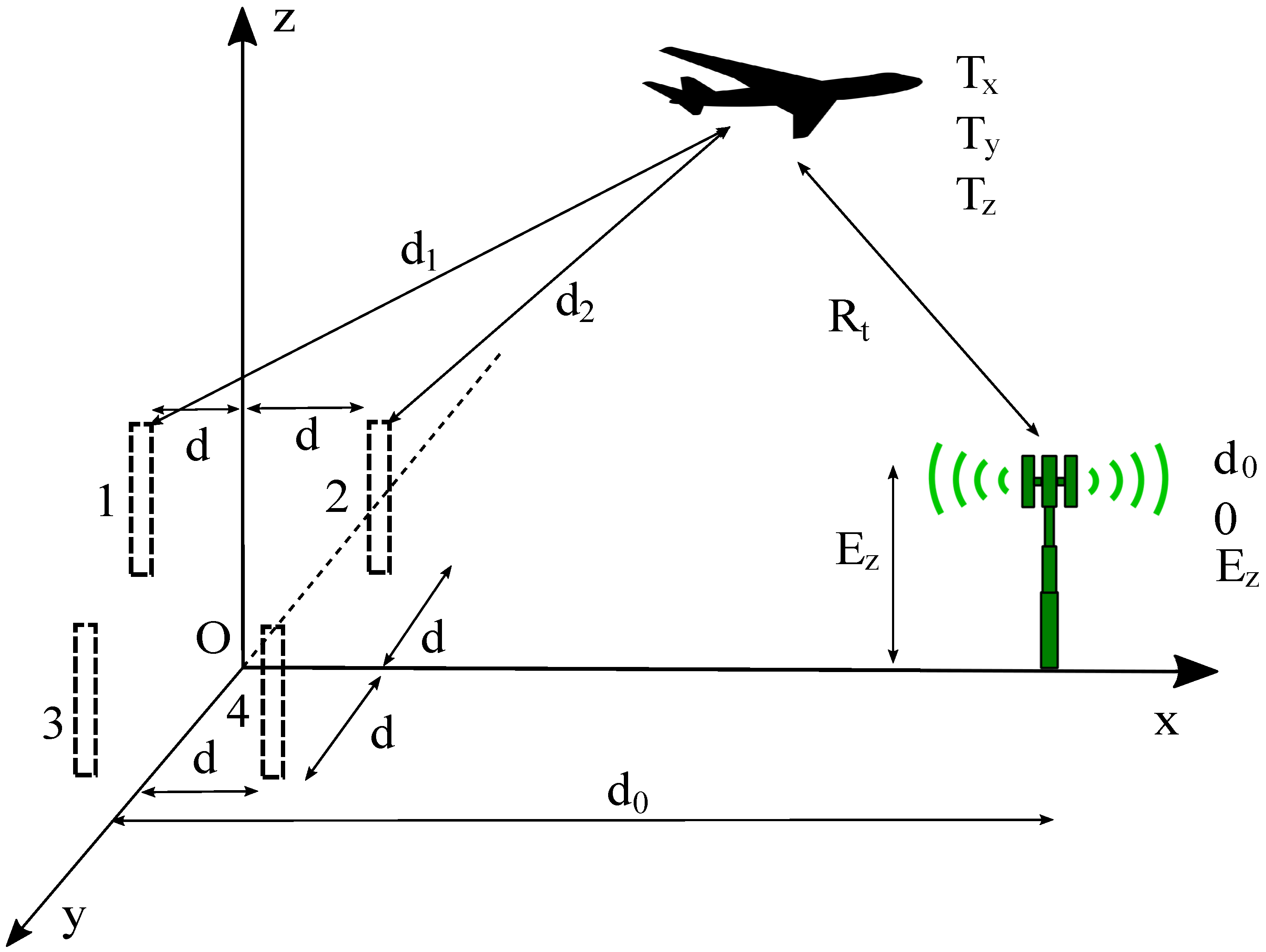
We first describe our scenario. As it is known, the DVB-T standard uses OFDM modulation for transmitting the signal. Typical modes are 2 K, 4 K, 8 K, 16 K, and 32 K, which correspond to the number of subcarriers, 2048, 4096, 8192, 16,384, and 32,768, respectively. However, not all the subcarriers are really sending information because some are reserved for pilots and guard frequencies. Let us consider a single DVB-T transmitter in an unknown position and a receiver equipped with four antennas, three of which are required for the algorithm whilst the fourth is used for calibration purposes. The four antennas are separated more than the wavelength to avoid electromagnetic coupling among them and thus achieve better performance. In general, the distance between antennas is $2d$, as indicated in Figure 1. As shown in this figure, the receiver establishes a coordinate system, with the origin in the middle of the four antennas. The primary reason for the four antennas is calibration. By using the signal received at all four antennas, the receiver can align with the transmitter and determine the distance $d_0$. During the calibration process, all four antennas are placed at the same height (z coordinate), but once the initial calibration is achieved, each of the four antennas is displaced into the z coordinate so that each one has a different value. This step is important in preventing the appearance of a rank-deficient matrix during operation. As can be observed, the DVB-T transmitter is located at a distance $d_0$ according to the new receiver-based coordinate system, and a height of $E_z$ with respect to the receiver. When a target appears, it will have the unknown coordinates $T_x$, $T_y$, and $T_z$.

Thus, the distance between the DVB-T transmitter and the target is denoted $R_t$, while the distance between the target and each of the receiver antennas is $d_i$ (with $i\in 1,2,3,4$). In the figure, only $d_1$ is depicted for clarity.

We seek to find the unknown coordinates of the target. In order to do this, we estimated the total distance $d{t}_i$ between the DVB-T transmitter and each of the antennas using the following formula [6]

$$R_t=\sqrt{{\left(T_x-d_0\right)}^2+T_y^2+{\left(Tz-E_z\right)}^2}$$

(1)

$$d_i=\sqrt{{\left(R{x}_i-T_x\right)}^2+{\left(R{y}_i-T_y\right)}^2+{\left(R{z}_i-Tz\right)}^2}$$

(2)

where $R{x}_i$, $R{y}_i$, and $R{z}_i$ are the coordinates x, y, and z, respectively, with respect to the receiver’s coordinate system of i-th antenna. Thus, the total distance to antenna i-th can be calculated as follows:

$$\begin{array}{c}d{t}_i=R_t+d_i=\hfill \\ \hfill \sqrt{{\left(T_x-d_0\right)}^2+T_y^2+{\left(Tz-E_z\right)}^2}+\sqrt{{\left(R{x}_i-T_x\right)}^2+{\left(R{y}_i-T_y\right)}^2+{\left(R{z}_i-Tz\right)}^2}\end{array}$$

(3)

The total distance $d{t}_i$ can be estimated, as will be explained in the following section. Assuming we have estimated those distances, after rearranging the equation, we obtain

$$\begin{array}{c}\hfill d{t}_i-\sqrt{{\left(T_x-d_0\right)}^2+T_y^2+{\left(Tz-E_z\right)}^2}=\sqrt{{\left(R{x}_i-T_x\right)}^2+{\left(R{y}_i-T_y\right)}^2+{\left(R{z}_i-Tz\right)}^2}\end{array}$$

(4)

By squaring both terms and making some straightforward calculations, we can obtain

$$\begin{array}{c}\left(R{x}_i-d_0\right)T_x+R{y}_i{T}_y+T_z\left(R{z}_i-E_z\right)-d{t}_i\sqrt{{\left(T_x-d_0\right)}^2+T_y^2+{\left(T_z-E_z\right)}^2}=\hfill \\ \hfill {\displaystyle \frac{1}{2}}\left(R{x}_i^2+R{y}_i^2+R{z}_i^2-d{t}_i^2-d_0^2-E_z^2\right)\end{array}$$

(5)

Using matrix notation, the above equation can be expressed as follows:  

$$\mathbf{S}\mathbf{x}=\mathbf{z}+\mathbf{r}{R}_t$$

(6)

where $\mathbf{x}={\left(T_x{T}_y{T}_z\right)}^T$, $\mathbf{r}={\left(d{t}_{1}d{t}_{2}d{t}_3\right)}^T$,

$$\mathbf{S}=\left(\begin{array}{ccc}(R{x}_1-d_0)& R{y}_1& (R{z}_1-E_z)\\ (R{x}_2-d_0)& R{y}_2& (R{z}_2-E_z)\\ (R{x}_3-d_0)& R{y}_3& (R{z}_3-E_z)\end{array}\right)$$

(7)

$$\mathbf{z}={\displaystyle \frac{1}{2}}\left(\begin{array}{c}(R{x}_1^2+R{y}_1^2+R{z}_1^2-d_0^2-E_z^2-d{t}_1^2)\\ (R{x}_2^2+R{y}_2^2+R{z}_2^2-d_0^2-E_z^2-d{t}_2^2)\\ (R{x}_3^2+R{y}_3^2+R{z}_3^2-d_0^2-E_z^2-d{t}_3^2)\end{array}\right).$$

(8)

Following least-squares (LS) estimation, $\mathbf{x}$ can be obtained as [31]

$$\widehat{\mathbf{x}}={\left({\mathbf{S}}^{\prime }\mathbf{S}\right)}^{-1}{\mathbf{S}}^{\prime }\left(\mathbf{z}+\mathbf{r}{R}_t\right)$$

(9)

Obviously, $R_t$ cannot be directly calculated but still needs to be estimated. Using spherical interpolation [6], $R_t$ can be estimated, minimizing the norm of the error $ϵ$

$$ϵ=\mathbf{z}+\mathbf{r}{R}_t-\mathbf{S}{\mathbf{S}}^{*}\left(\mathbf{z}+\mathbf{r}{R}_t\right)=\left(\mathbf{I}-\mathbf{S}{\mathbf{S}}^{*}\right)\left(\mathbf{z}+\mathbf{r}{R}_t\right)$$

(10)

where ${\mathbf{S}}^{*}={\left({\mathbf{S}}^{\prime }\mathbf{S}\right)}^{-1}{\mathbf{S}}^{\prime }$. We may the define $\mathbf{T}=\mathbf{I}-\mathbf{S}{\mathbf{S}}^{*}$, and since $\mathbf{T}$ is symmetrical and idempotent:

$$R_t=-{\displaystyle \frac{{\mathbf{r}}^{\prime }\mathbf{T}\mathbf{z}}{{\mathbf{r}}^{\prime }\mathbf{T}\mathbf{r}}}$$

(11)

After $R_t$ is estimated, it can be used in Equation (9) to produce the final estimation of the target coordinates.

The next section provides a detailed description of the proposed algorithm, which first estimates the total distances to each antenna ($d{t}_i$), and then refines the estimation through an iterative procedure.

3. Proposal Description

The flowchart of our proposal is depicted in Figure 2.

As explained in the previous section, the estimation of the total distance to each antenna $\widehat{d_i}$ is required before converting them into Equations (8), (9), and (11).

3.1. Calibration Process

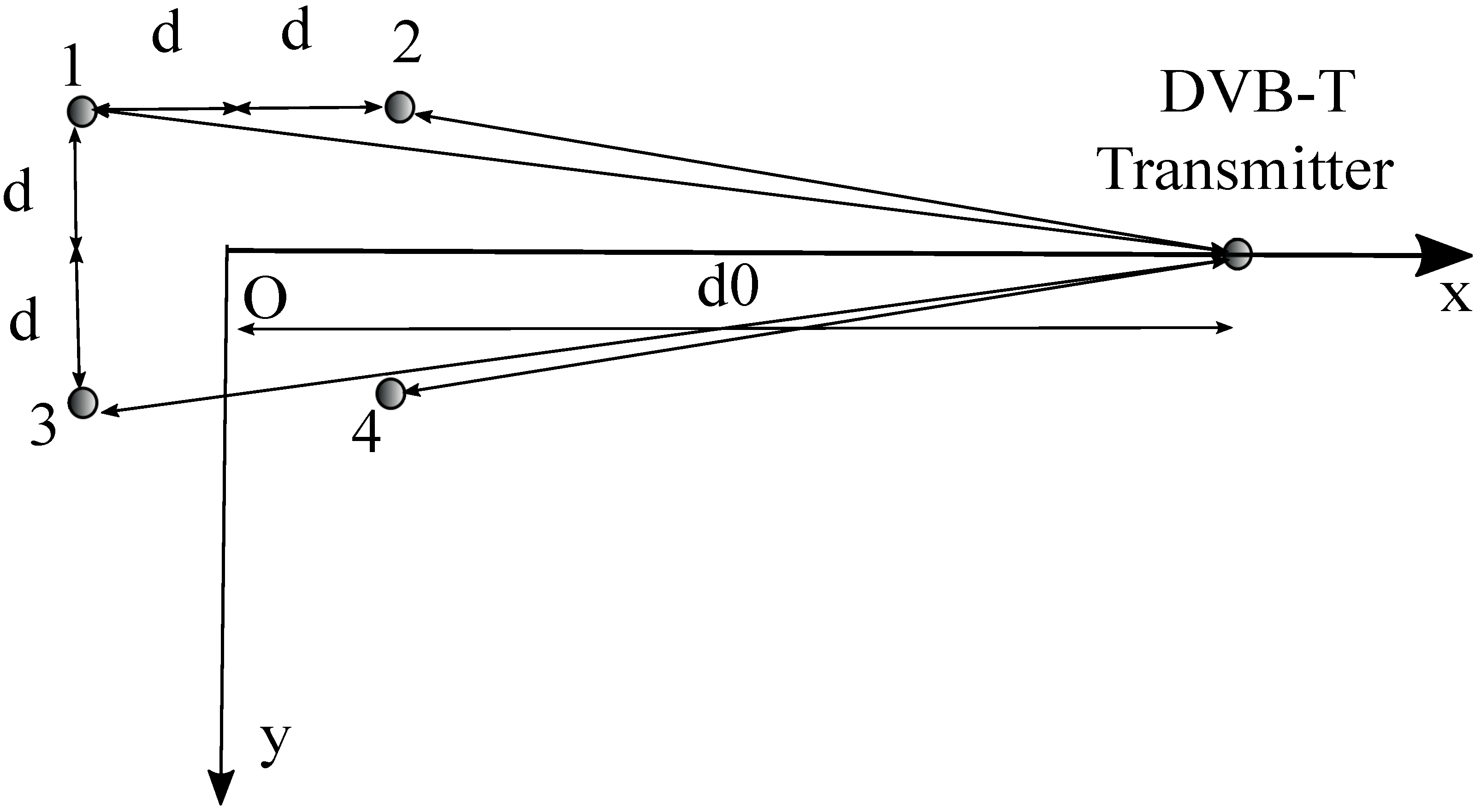
Before performing the estimation, the system must be calibrated. The calibration will identify the distance to the transmitter, $d_0$ and the height with respect to the receiver, $E_z$. As explained earlier, this method will estimate a target’s position with respect to the center of the receiver, i.e., O; as a consequence, the obtained coordinates are not absolute but relative to the center of the receiver. First of all, the x axis is determined as follows. As seen in Figure 3, which is a top–down view of Figure 1 without the target, the x axis is the line between the center of the receiver and the transmitter when the four antennas that receive the signal are perfectly aligned. In order to achieve alignment, all four antennas are positioned at the same height, and the receiver is moved (rotated) until the signal is received at antennas 2 and 4 at the same time, and signal at antennas 1 and 3 are received at the same time and delayed with respect to the others.

Once the axis x is determined, the receiver synchronizes with the DVB-T transmitter, after which the distance $d_0$ and height $E_z$ can be estimated. If the receiver used the global positioning system (GPS), the GPS coordinates of the transmitter $d_0$ and $E_z$ can be easily obtained; alternatively, if such coordinates are lacking, the receiver can proceed as follows. Since the receiver is synchronized with the DVB-T transmitter, it can estimate the time of arrival of the signal, and with this value, it can estimate the initial distance $l_0$. Then, the receiver is moved a known distance $\mathrm{\Delta }$ along the y axis and the time of arrival is again calculated in the new position in order to estimate the second distance $l_f$. With these two distances, and some simple similarity mathematics, the values of distance $d_0$ and height, $E_z$ can be obtained as follows:

$$\left.\begin{array}{c}{l}_0^2=E_z^2+d_0^2\hfill \\ l_f^2=E_z^2+{\left(d_0+\mathrm{\Delta }\right)}^2\hfill \end{array}\right\}$$

(12)

Consequently, the solution is   

$$\left.\begin{array}{c}{d}_0={\displaystyle \frac{l_f^2-l_0^2-{\mathrm{\Delta }}^2}{2\mathrm{\Delta }}}\hfill \\ E_z=\sqrt{l_0^2-d_0^2}\hfill \end{array}\right\}$$

(13)

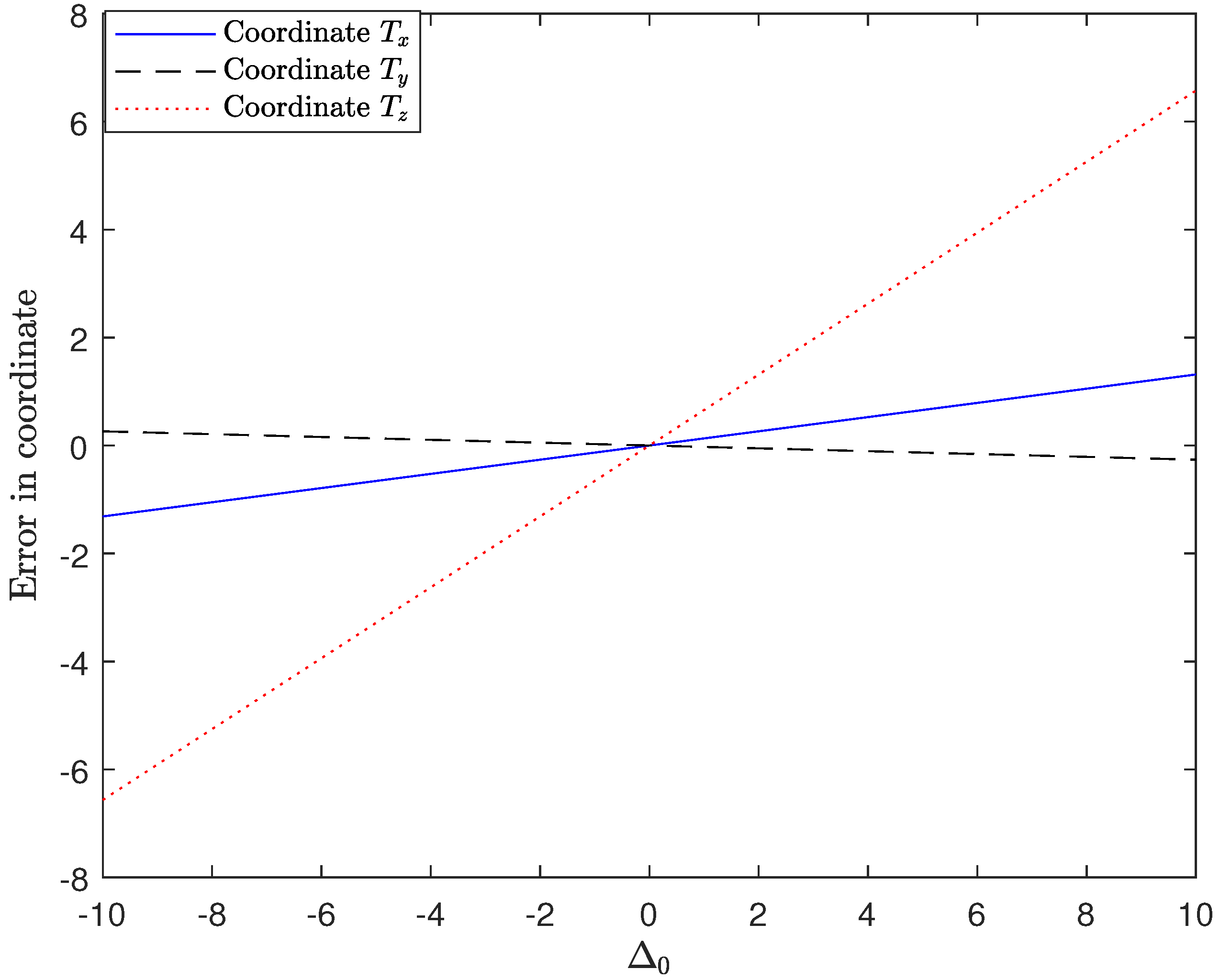
Although the errors in the estimation of these two parameters—$E_z$ and $d_0$—in the calibration process is small, in the following, we have analyzed the impact on the final estimation error in the different coordinates, even for large errors in their estimation.

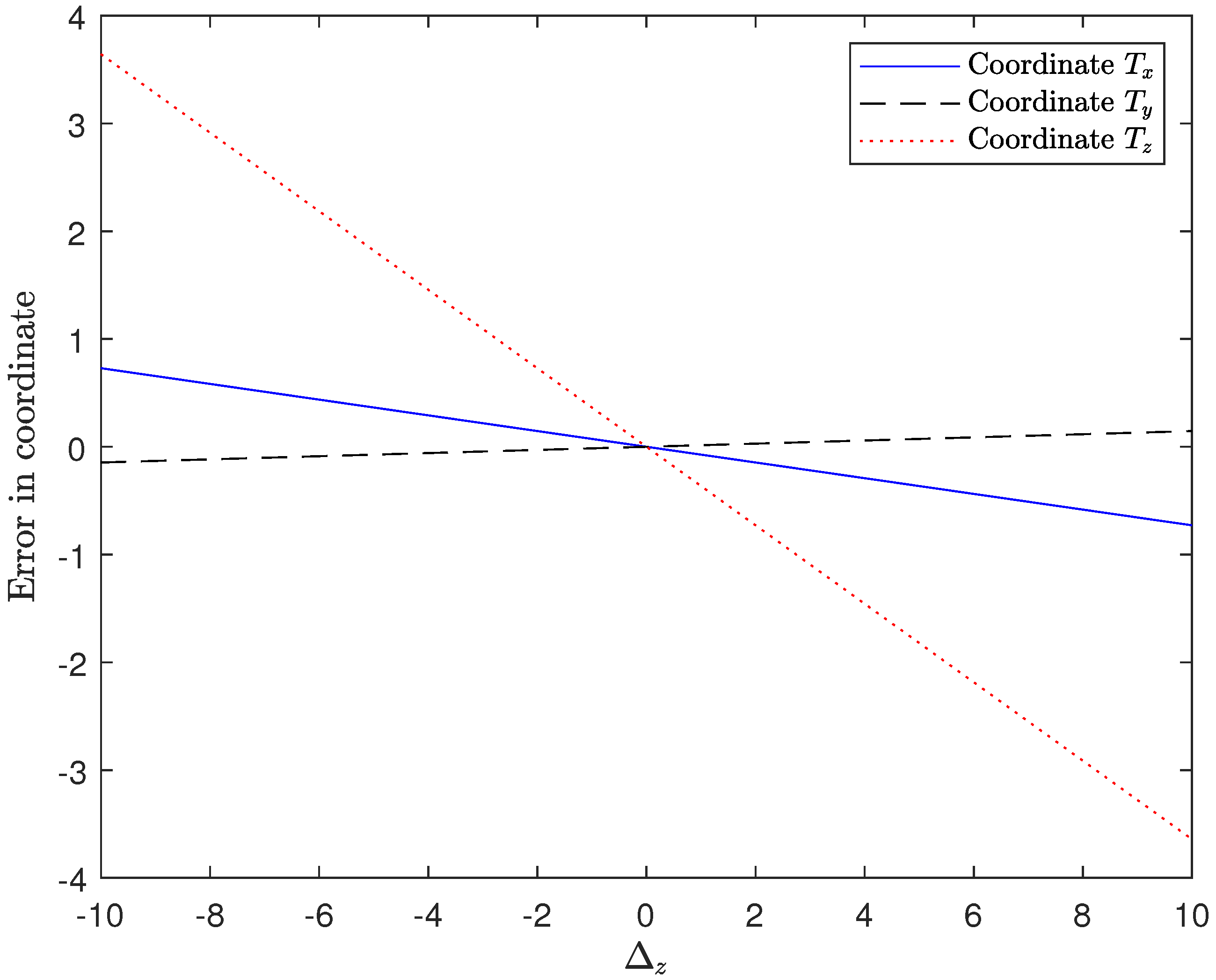
Let us assume that there is some error in $E_z$ and $d_0$ in the form of $E_z^{\prime }=E_z+{\mathrm{\Delta }}_z$ and $d_0^{\prime }=d_0+{\mathrm{\Delta }}_0$, respectively. In Figure 4 and Figure 5, the final estimation error of each of the three coordinates is depicted. The error ${\mathrm{\Delta }}_0$ or ${\mathrm{\Delta }}_z$ is indicated in meters. Typically, this misalignment is only several centimeters, i.e., much lower than 1 m, but we have explored the behavior with errors up to $\left|10\right|$ meters. As it can be seen in Figure 4, when ${\mathrm{\Delta }}_z=0$ (no error in $E_z$), the effect over the different coordinates $T_x,T_y$ and $T_z$ is proportional to the error in $d_0$, ${\mathrm{\Delta }}_0$. It can also be observed that the effect on coordinate $T_y$ is very small, almost negligible even for large values of ${\mathrm{\Delta }}_0$, while the impact on $T_z$ is more important. The reason is that the calculations for coordinate $T_y$ involving either $E_z$ or/and $d_0$ are much fewer compared to the other two coordinates that make use of them several times (see Equations (7)–(9)).

Similar behavior can be observed when we evaluate the error is $E_z$ with ${\mathrm{\Delta }}_0=0$, but the proportional values are slightly different. Interestingly, the impact on the error on each coordinate is being balanced between ${\mathrm{\Delta }}_0$ and ${\mathrm{\Delta }}_z$. This is, when the effect of ${\mathrm{\Delta }}_0$ is positive, the one in ${\mathrm{\Delta }}_z$ is negative, so they can be compensated each other for some values.

Looking at the results, the impact on coordinates $T_x,T_y$ and $T_z$ is $0.13137{\mathrm{\Delta }}_0$−$0.07291{\mathrm{\Delta }}_z$, $-0.026269{\mathrm{\Delta }}_0$ + $0.014579{\mathrm{\Delta }}_z$ and $0.65646{\mathrm{\Delta }}_0$−$0.3643{\mathrm{\Delta }}_z$, respectively.

Finally, if those error are smaller than 1 m, what is easy to obtain, the error in the final estimation is negligible.

After this initial calibration, the system is ready for operation, although a few more steps are needed to complete its setup. The first step is to move in the z axis the position of each antenna on the z axis so that each one has a different height $R{z}_i$ (as explained earlier). This step will prevent the occurrence of a rank-deficient matrix in the estimation process. After these easy and simple steps, the receiver is initialized and ready for estimation.

3.2. Channel Estimation

During the idle period, i.e., the time in which there is no target within the scenario, the received DVB-T signal is processed at each antenna. As indicated earlier, not all the available subcarriers are transmitting information. Depending on the configuration, there are some subcarriers reserved for the transmission of pilots (known signals at both sides to estimate the channel or synchronize the frame). Using the pilot structure of the signal (see Figure 6 [27] or [28], channel estimation is performed using LS in the frequency-domain. As shown in this figure (the pilot pattern PP1 in DVB-T2 is the same), in the frame structure, at sub-carrier 0, there is always a pilot (a known signal) throughout the whole transmission frame, denoted as the edge pilot (in DVB-T2, it is denoted as the closing frame symbol and it is the same); other scattered pilots throughout the frame swipe their position during frame transmission in order to cover the whole bandwidth (in DVB-T2, there are eight different pilot patterns). In general, the number of pilots per OFDM symbol depends on the FFT size (2 K, 8 K, or even 4 K, 16 K, or 32 K for DVB-T2) and configuration, and the percentage varies from the standard and the FFT size.

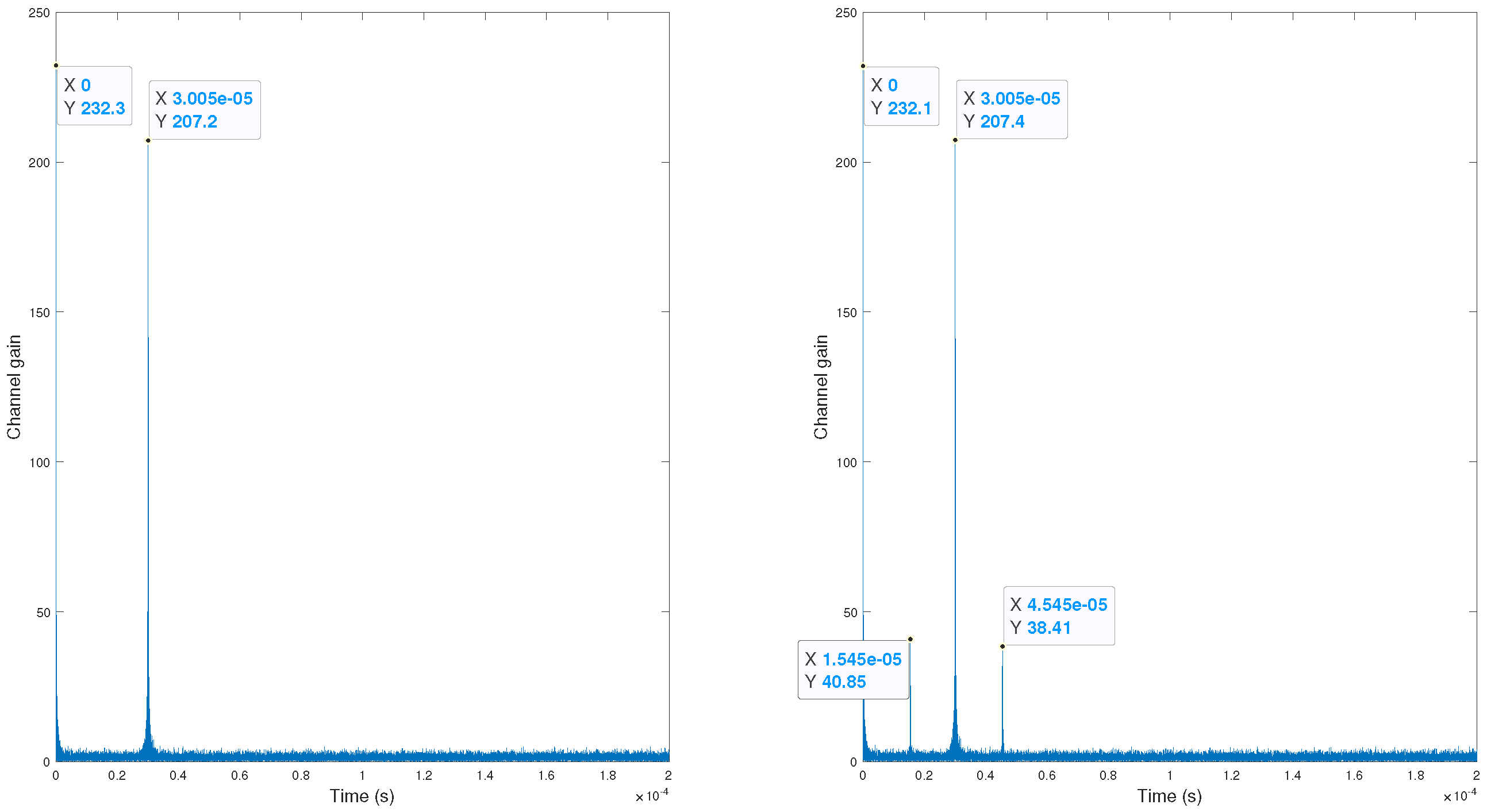
Afterwards, the time-domain version is calculated by applying the inverse fast Fourier transform (IFFT) to the estimated channel to obtain $\widehat{{\mathbf{h}}_{\mathbf{i}}}$. These calculations are continuously being estimated and used as reference. This time-domain estimation is similar to the power-delay profile of the system wherein the taps (reflections) of the channel can be identified. Using these taps (and the time), the different reflections can be observed.

The LS channel estimation summarized above can be mathematically described as follows. Let ${\mathbf{a}}^{\mathbf{i}}\in {\mathbb{C}}^{1\times L}$ be the received time-domain signal at the i-th antenna and ${\mathbf{A}}^{\mathbf{i}}\in {\mathbb{C}}^{1\times L}$ be its frequency-domain signal. Within this ${\mathbf{A}}^{\mathbf{i}}$, the values at pilot positions $\mathcal{K}$ are denoted as ${\mathbf{P}}_{\mathcal{K}}$. The channel at pilot positions can be estimated using zero-forcing [32]:

$${\widehat{\mathbf{H}}}_{\mathcal{K}}^{\mathbf{i}}={\displaystyle \frac{{\mathbf{A}}_{\mathcal{K}}^{\mathbf{i}}}{{\mathbf{P}}_{\mathcal{K}}}}$$

(14)

Since only the channel is estimated at the pilot position, an interpolation process is required. In this case, simple low-pass filtering is used. Zeros are inserted in the data positions ($\notin \mathcal{K}$) before the resulting new vector goes through a low-pass filter, meaning that known values stay equal and unknown values (zeros) are interpolated between unchanged data such that the mean-square error between the interpolated points and their ideal values are minimized [33]. Finally, the time-domain version of the estimated channel is calculated alongside its IFFT (see Figure 7).

3.3. Operational Time

During the operational time, at each frame, the channel is estimated at each antenna, and the power delay profile (PDP) is obtained for each antenna.

When a target appears, it is likely that the reflections into this channel will affect its propagation characteristics, causing the channel’s estimation to change and new reflections (taps) to appear in the estimation of time-domain channel, as shown in Figure 7 for receiver antenna 2 (all antennas will exhibit similar behavior). In this figure, the PDP is the plot. As shown in this figure, a multi-path channel with two taps is simulated without any target on the left side, and with the target on the right side. This channel may appear in a scenario in which there is a main reflector (clutter) like a building or a mountain. Thus, by comparing both estimations, new taps can be identified. For the purposes of localization, the first new tap (${\tau }_n$) will make the main contribution to the target reflection; thus, we chose to use it because our goal is to estimate its position and not to identify the channel for coherent demodulation. At this point, it is notable that, for our proposal, the important value to take into account is the delay in the new tap in inferring the total distance to this antenna, and not the amplitude. Thus, we can consider the time of this first new tap to be the time of arrival for the reflection on the target; then, assuming the speed of the light (c), we can calculate the distance using $d=c\times {\tau }_n$. It is important to note that, in more complex scenarios with multiple clutters, since the algorithm operates based on the difference in PDP, the first new tap also provides a reliable estimate for the target’s distance.

Once we have estimated the three total distances to each antenna, the Equation (9) can be used to estimate the position. If our estimations of the distances were perfect, Equation (9) would provide the exact coordinates of the target. However, small mismatches in the distances will result in erroneous estimations. Indeed, this equation is quite robust if the distance to the antenna is large. For example, if the antennas are separated by several km, this formula only produces minimal errors, even for errors of 10 or more meters in the estimation of distances. This is the case when several receivers are used and has been extensively evaluated in the existing literature. The reason behind is that the error on distances compared to the distance between antennas is small. However, it is usually challenging to use several synchronous receivers for this purpose. In our design of a compact receiver with antennas separated by a few meters, an error of even 1 m has the same order of magnitude as the distances between antennas. Therefore, the impact on the estimation accuracy is huge. Looking at Equation (10), two factors can be easily identified. The first involves a pseudo-inverse and identity matrix, which only depends on the coordinates of the antennas and their distances from the transmitter ($d_0$) and its height, $E_z$; it is essentially a $1/2$ factor (in matrix form). The second part of the expression depends on $\mathbf{z}$, $\mathbf{r}$, and $R_t$. Examining $\mathbf{z}$ in more detail, we can see that whether the antennas are co-located, the coordinates $R{x}_i,R{y}_i$, and $R{z}_i$ will be small in comparison to $d_0$ and $d{t}_i$; thus, the vector will be dominated by $d_0^2$ and $d{t}_i^2$. A similar reasoning applies to $\mathbf{r}{R}_t$, which is also dominated by $d_0^2$ and $d{t}_i^2$. If the error in the distance at each antenna is denoted by ${\mathrm{\Delta }}_i$, even for small values of ${\mathrm{\Delta }}_i$, these values will be high. On the other hand, if the antennas are not co-located, the $R{x}_i$, $R{y}_i$, and $R{z}_i$ coordinates with respect to the theoretic hypothetical origins of coordinates in the center of the different antennas will be comparable to $d_0$ and $d{t}_i$. Consequently, $ϵ$ will be small, even for reasonably large error values.

In order to reduce the error in the estimation of coordinates, the estimation of the distances is refined based on the error in the coordinates. Small errors in distances generate large errors in estimation; to compensate for this drawback, we designed an algorithm to refine these distances for the estimation of true positions. Taking the initial distances estimated by the channel as the starting point, this algorithm slightly modifies (i.e., increases or decreases) them (each coordinate estimate), and the error of this change is evaluated. After some analysis, we acknowledge that the optimal solution is to choose the change that has minimal impact on the estimated error (causing minimum dispersion); this change is safer than any other. Since the formula is quite sensible to errors, strategies such as gradient descent using a Jacobian [34] method would produce incorrect estimations and large errors.

3.4. Iterative Algorithm

The pseudo-code for the algorithm is described in Algorithm 1, where the matrix that includes the possible changes (updates) at each of the three distances is  

$$\mathbf{M}=\left(\begin{array}{cccccc}1& -1& 0& 0& 0& 0\\ 0& 0& 1& -1& 0& 0\\ 0& 0& 0& 0& 1& -1\end{array}\right)$$

(15)

Although the pseudo-code of the algorithm in Algorithm 1 encompasses all the steps and mathematical formulations, a concise summary of the process is provided below.

Algorithm 1 Refinement of coordinates’ estimation.

1: Initialization:  2: Calculate $\widehat{R_t}$ using Equation (11) using estimated distances $\widehat{\mathbf{r}}={\left(\widehat{d{t}_1}\widehat{d{t}_2}\widehat{d{t}_3}\right)}^T$ instead of $\mathbf{r}$  3: Calculate $\widehat{\mathbf{x}}$ using Equation (9) and $\widehat{R_t}$  4: $epoch=1$  5: Re-calculate estimated distances using estimated coordinates $\widehat{\mathbf{x}}$: $$\begin{array}{c}\hfill \tilde{\mathbf{r}}=\sqrt{{\left(\widehat{T_x}-d_0\right)}^2+{\widehat{T_y}}^2+{\left(\widehat{T_z}-E_z\right)}^2}+\sqrt{{\left(R{x}_i-\widehat{T_x}\right)}^2+{\left(R{y}_i-\widehat{T_y}\right)}^2+{\left(R{z}_i-\widehat{T_z}\right)}^2}\end{array}$$  6: Calculate the total error: ${ϵ}_T=\left|\right|\widehat{\mathbf{r}}-\tilde{\mathbf{r}}{\left|\right|}^2$  7: while ${ϵ}_T\le TargetError$ AND $epoch<MaxEpochs$ do                                       ▹ Stop condition  8:     $epoch++$  9:     for $j=1:6$ do 10:         $\mathbf{m}=\mathbf{M}[:,j]$                                                                   ▹ Select the dimension to modify 11:         ${\tilde{\mathbf{r}}}^j$ = $\tilde{\mathbf{r}}+\mathbf{m}·\mu$                                                                ▹ Update estimation of distances 12:         Calculate ${\widetilde{R_t}}^j$ using Equation (11) using modified distances ${\tilde{\mathbf{r}}}^{\mathbf{j}}$ instead of $\mathbf{r}$ 13:         Calculate ${\tilde{\mathbf{x}}}^{\mathbf{j}}$ using Equation (9) and ${\widehat{\widetilde{R_t}}}^j$ 14:         Calculate new distances ${\widetilde{\tilde{\mathbf{r}}}}^j$ using Equation (3) assuming ${\tilde{\mathbf{x}}}^j$ instead of $\mathbf{x}$ 15:         Evaluate the distance error: ${\mathit{ϵ}}^j={\left({\tilde{\mathbf{r}}}^j-{\widetilde{\tilde{\mathbf{r}}}}^j\right)}^2$                 ▹ Evaluate error for this choice 16:     end for 17:     Sort ascending $\mathit{ϵ}$: ${\mathit{ϵ}}_{sorted}$ 18:     Calculate the difference between largest and lowest: 19: ${\mathit{ϵ}}_{diff}={\mathit{ϵ}}_{sorted}\left(3,:\right)-{\mathit{ϵ}}_{sorted}(1,:)$                                                            ▹ Maximum - Minimum 20:     $idx=min{ϵ}_{diff}$                                                                    ▹ Select the one that minimizes 21:     Update: 22:     $\tilde{\mathbf{r}}={\tilde{\mathbf{r}}}^{idx}$                                                                                   ▹ Update estimated distances 23:     ${ϵ}_T=\left|\right|\widehat{\mathbf{r}}-\tilde{\mathbf{r}}{\left|\right|}^2$                                                                     ▹ Update total error with choice 24: end while 25: OUTPUT: $\widehat{\mathbf{x}}$ using Equation (9) with $\tilde{\mathbf{r}}$

Initially, during the algorithm’s initialization phase, the estimated distances, ${\widehat{dt}}_i$, obtained from the channel estimation process, is used to estimate the target coordinates, $\widehat{\mathbf{x}}$, as described in Equation (9). Equation (11) is applied to estimate $\widehat{R_t}$, which, along with steps 2 and 3, yields the initial coordinate estimate, $\widehat{\mathbf{x}}$.

Next, the algorithm calculates the expected distances, ${\widetilde{dt}}_i$, assuming that the target coordinates are the previously estimated coordinates, $\widehat{\mathbf{x}}$, resulting in a distance vector $\tilde{\mathbf{r}}$. Using these estimated distances, the total estimation error, ${\mathit{ϵ}}_T$, is computed in step 6. This error is used both for iteration and to determine the stop condition.

The algorithm iterates until the stop condition is met, either when the total error, ${\mathit{ϵ}}_T$, satisfies the condition ${\mathit{ϵ}}_T\le TargetError$ or when the maximum number of iterations is reached.

For each iteration, the algorithm computes six coordinate sets, ${\widehat{\mathbf{x}}}^j$, by making small adjustments to one of the estimated distances, ${\widehat{dt}}_i^j$, either increasing or decreasing it [step 11]. The coordinates, ${\widehat{\mathbf{x}}}^j$, are then estimated with these modified distances [steps 12 and 13]. Subsequently, the corresponding distances, ${\tilde{\mathbf{r}}}^j$, are recalculated based on the modified coordinates [step 14], and the total error for each combination is evaluated [step 15]. The combination producing the smallest change is selected as the updated values for the estimated distances [steps 18–22] because it is the safer one. Finally, the total error is computed with these updated distances in step 23, and the stop condition is checked using this new total error, ${\mathit{ϵ}}_T$.

Upon completion, the algorithm outputs the final coordinate estimates, derived from the updated distances.

For example, the first column in $\mathbf{M}$ is represented in the algorithm by $\mathbf{m}=\mathbf{M}[:,1]$ and shows how many of the three distances are changed. This first column in $\mathbf{M}$ indicates that only the first distance is modified. $\mu$ is the update factor. Notably, larger values of $\mu$ converge more rapidly; however, since these values are produced during the updating step, the granularity and resolution decrease, and a highly probable erroneous estimation is given. For example, if the initial error is of 1.5 m, an update of 0.1 m or 0.3 m will produce zero-error, but an update of 0.2 will leave a remainder error. On the contrary, smaller values will produce a slower convergence but better resolution. If we denote the remainder error ${\delta }_i$, which is essentially the non-divisible part of the error with respect to $\mu$, and recall our on the analysis of $ϵ$ in the previous sections, the total error of the algorithm will be proportional to ${\delta }_i^2$. Eventually, there is a trade-off between speed and resolution.

It worth nothing to indicate that the proposal can be applied to the DVB-T2 standard, only replacing the structure of the frame and the pilots for the channel estimation process.

3.5. Complexity Analysis

In terms of time complexity analysis, assuming that matrix inversions are performed using the most efficient algorithm based on p-adic expansions, which exhibits a complexity of $𝒪\left(3^3{log}^{2}3\right)=𝒪\left(6.14\right)$, the square matrix multiplications are carried out using Strassen’s algorithm, with a complexity of $𝒪\left(3^{2.807}\right)=𝒪\left(21.84\right)$. For the non-square matrix multiplication of the form $A^{M\times N}\times B^{N\times P}\times C^{P\times M}$, the Naive algorithm is employed, with a complexity of $𝒪\left(M·N·P+M^2·P\right)$. The sorting algorithm used is the tree-sort, which is based on the Binary Search Tree and has a complexity of $𝒪\left(6log6\right)=𝒪\left(4.69\right)$. The time complexities of the various steps in the algorithm are as follows:

• Step 2: $3𝒪\left(12\right)$
• Step 3: $3𝒪\left(21.84\right)+𝒪\left(6.14\right)+𝒪\left(9\right)$
• Step 5: $𝒪\left(20\right)$
• Step 6: $𝒪\left(4\right)$
• Each epoch:

  –

  6 times:

  *

  Step 11: $𝒪\left(6\right)$

  *

  Step 12: $3𝒪\left(21.84\right)+𝒪\left(6.14\right)+𝒪\left(9\right)$ like step 3

  *

  Step 14: $𝒪\left(20\right)$ like step 5

  *

  Step 15: $𝒪\left(6\right)$

  –

  Step 17: $𝒪\left(4.69\right)$

  –

  Step 19: $𝒪\left(6\right)$

  –

  Step 23: $𝒪\left(4\right)$

In any case, such a degree of complexity is linear and affordable for simple devices. For example, for a simple Raspberry Pi of 4.4 giga floating point operations per second (GFLOPS), in the worst case, in which 10k iterations are needed, the algorithm will take approximately 1 ms to complete them.

3.6. SFN Considerations

A single-frequency network (SFN) is a transmission scenario where multiple transmitters broadcast the same signal on the same frequency. This is commonly used in DVB-T and DVB-T2 systems. The key advantage of SFN is that it allows for the coverage of large areas with a reduced spectrum usage. In an SFN, all transmitters are synchronized to transmit the same signal at the same time, effectively minimizing interference between them and providing robust reception over a wide geographical region.

However, implementing SFN in DVB-T or DVB-T2 systems involves addressing several technical challenges. One of the most significant hurdles is ensuring that the transmission signals from different transmitters remain time-aligned. Any misalignment can cause inter-symbol interference (ISI), which degrades the quality of the reception. The synchronization process relies on precise timing, which can be influenced by factors such as the distance between transmitters, network topology, and the stability of the clocks used in each transmitter.

To mitigate these challenges, DVB-T and DVB-T2 systems utilize time–frequency synchronization techniques. These techniques ensure that the signals transmitted from different transmitters are synchronized, maintaining signal coherence and reducing potential interference. Furthermore, advanced error correction mechanisms, such as forward error correction (FEC), are often employed to enhance signal robustness in SFN environments. Additionally, there are some limitations on the maximum distance those multiple transmitters can be. In order to avoid multipath problems, a guard interval (GI) is left to absorb the echoes and avoid ISI. This GI is flexible and will depend on the scenario. The longest GI in DVB-T is 224 (1/16 of the OFDM symbol period) $\mathsf{\mu }$s and in DVB-T2 is 532 $\mathsf{\mu }$s (19/128). If the signal from other transmitters arrive with a delay longer than this, it will not be canceled by GI and will appear as interference and the synchronization process will fail too. Thus, the maximum distance for the other transmitters when SFN configuration is used is around 67 km and 160 km for DVB-T and DVB-T2, respectively.

In terms of performance, SFN provides several benefits. It enables seamless coverage across large areas with minimal gaps or overlaps between transmission zones, improving signal availability, especially in urban environments or rural areas with challenging terrains. Moreover, SFN allows broadcasters to economize on spectrum usage, making more efficient use of available frequencies.

On the flip side, managing SFN in DVB-T and DVB-T2 systems requires the careful planning of transmitter locations, transmission power levels, and the timing synchronization of the entire network. Additionally, the multipath effects caused by the reflection of signals off buildings or natural obstacles can lead to destructive interference, particularly when the signals from multiple transmitters arrive at the receiver at slightly different times.

Regarding our system in SFN configuration, since the initialization phase estimates the channel without targets, it will also characterize the possible echoes from other transmitters and thus, this configuration does not affect the performance.

4. Results and Discussion

In order to evaluate our proposal, we present several simulations. In all of them, the DVB-T transmitter has an equivalent isotropic radiated power (EIRP) of 20 dBW and the noise level is adjusted to the specified signal-to-noise ratio (SNR). The target is placed in different positions, as is the receiver. The distance between antennas at the receiver is $d=2.55$ m and the three antennas (1,2,3) are moved 1, 2, and 3 m along the z axis once the calibration is finished in order to avoid the occurrence of a rank-deficient matrix S. The frequencies used were 482, 530, and 626 MHz (if applicable). The other parameters of this simulation can be found in

Table 1. System parameters.

Symbol	Description	Value	Units
	Standard	8k	-
$P_{tx}$	Transmission power	20	dBW
$f_c$	Transmission frequency	482, 530, 626	MHz
$N_c$	N. of useful subcarriers	6817	-
$T_u$	Useful symbol duration	896	$\mathsf{\mu }$s
$T_s$	OFDM symbol duration	1120	$\mathsf{\mu }$s
B	Bandwidth	7.61	MHz
d	Distance between antennas	2.55	m
$d_0$	Distance to DVB-T Tx	[1–10]	km
$T_z$	Target altitude	[1–15]	km
$T_x$, $T_y$	Target coordinates	[1–30]	km
$\mu$	Update factor	0.015	m
L	Max. n. of iterations	10,000	-
K	Upsampling factor	10	-
$\delta$	Target error	0.1	m
$E_z$	Tx height	10	m
${\alpha }_t$	Target’s reflection coefficient	0.9	-
DS	Doppler spectrum	Jakes	-

. Although parameter d does not directly affect the algorithm, it is important to highlight that the distance between antennas is $2d$. In order to achieve diversity, a separation of at least $\lambda /4$ or $\lambda /2$ is needed. However, within traditional estimation algorithms, the larger this distance is, the better the performance and the lower the permissible error, as indicated earlier in this paper. For this reason, to maintain a compact design, a value of approximately 10 times the wavelength of the frequency range is used.

To clarify the simulation process, the procedure for generating each realization is outlined below. The first step is to randomly generate the distance from the transmitter (Tx), denoted as $d_0$, within the range of 1 to 10 km. As specified in Table 1, the Tx’s height is set to 10 m, which is a typical value for a DVT-T transmitter. Next, a random channel is generated between the Tx and the four receiver (Rx) antennas, with some correlation considered among the antennas.

Following this, a target is placed at a random position within the specified range (see Table 1). The channel with the target present is then calculated, taking into account potential reflections. The path loss between the Tx and each antenna is determined. To simulate the adequate signal-to-noise ratio, the noise value is calculated to achieve the desired SNR. If, due to the randomness of positioning, the value generated cannot meet the desired SNR value, this position is discarded and another one is generated (e.g., the SNR being simulated is very high and the random position for Tx and Target only with the path loss exceeds the SNR, and thus, noise should be negative to reach the desired value. In this case, another position is randomly generated). Additionally, the path loss between the Tx and the target, as well as between the target and the antennas, is computed.

For each realization, eight frames (approximately 600 ms) are simulated using the same channel. The channel at each antenna is estimated using pilot sequences within the signal, and the power delay profile is obtained. The same procedure is repeated with the target included in the simulation. Next, the difference between the PDPs is calculated, and the distances are estimated. Finally, the algorithm is applied to refine the estimated coordinates based on these initial distance estimates. As indicated, the algorithm runs until the $TargetError$ is met (0.1 m) or the maximum number of iterations is reached (10,000).

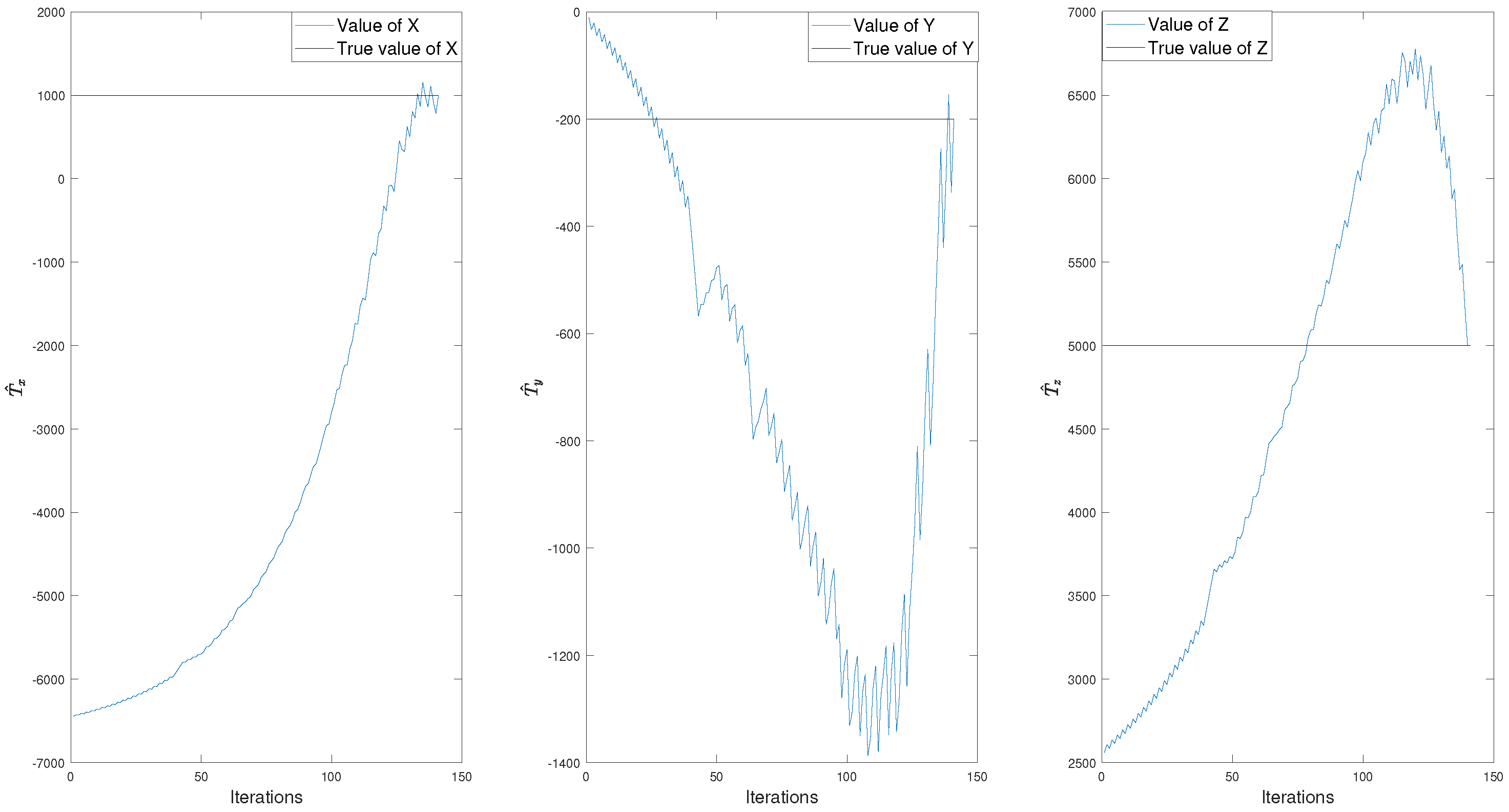
In Figure 8 and Figure 9, the evolution of the coordinates’ estimation and the evolution of the error at each distance as the iterations progress are shown in a synthetic example, wherein the estimated distances 1, 2, and 3 exhibited a relatively large error of 30, 60, 50 m, respectively, that is, if the theoretical estimated distance at antenna 1 is 1000 m, it estimates 30 more meters. As shown in Figure 8, for example, the original estimation is completely erroneous when the error in the estimated distances is large; eventually, however, they converge to the correct estimation at the end due to the refinement process. Interestingly, this convergence is not monotonous. This is one of the reasons that Jacobian descent and other similar methods cannot adequately address this problem. In Figure 9, the evolution of the error in the estimation of the three distances with respect to the true distance is shown (${\mathrm{\Delta }}_i=d{t}_i-{\widehat{dt}}_i$). 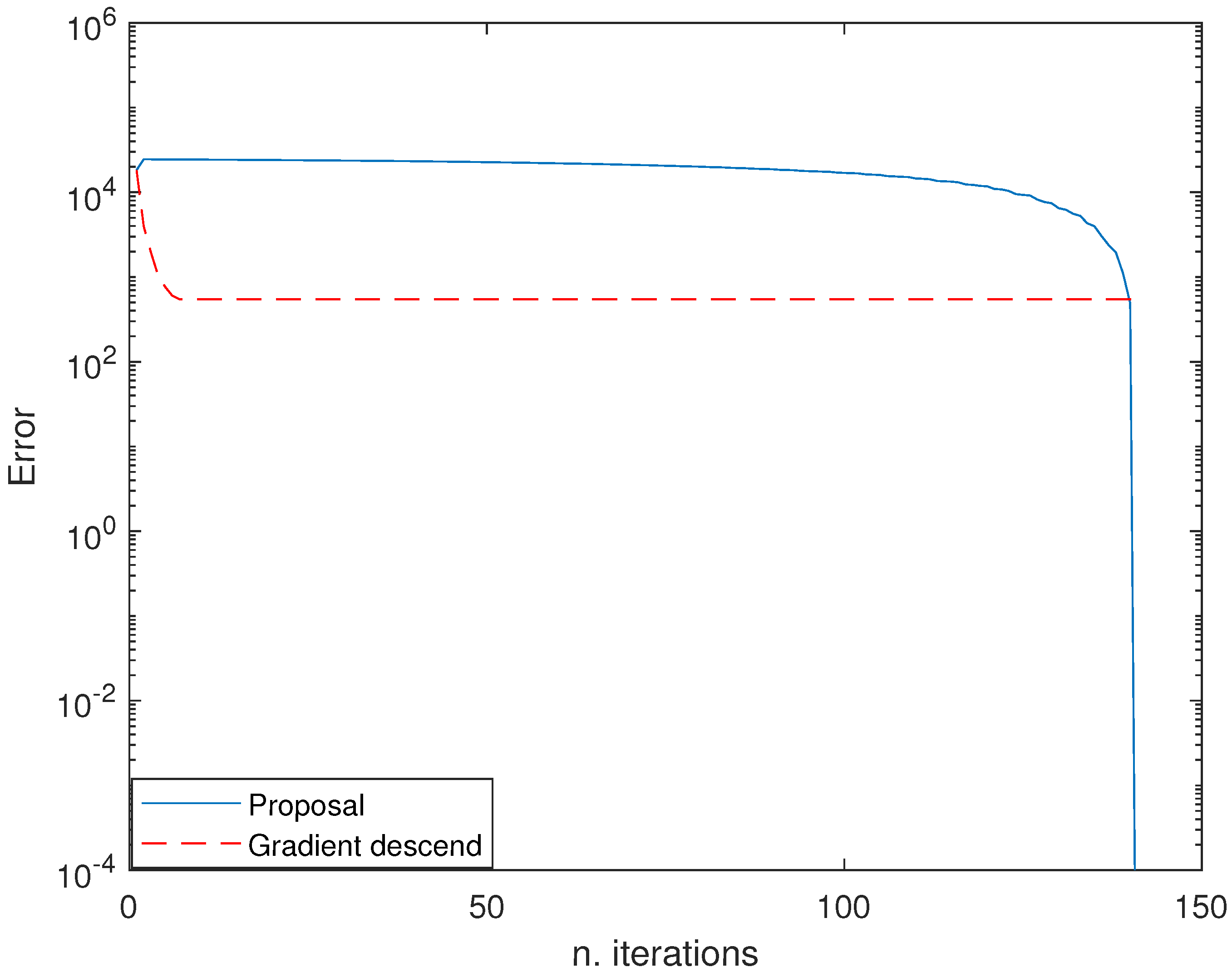In this figure, the y axis shows the estimated error at each antenna during the running of the algorithm. At the beginning, the first antenna showed an error of 30 m, antenna 2 showed an error of 60 m, and antenna 3 showed an error of 50 m. These errors converge gradually to the true value, i.e., as it can be seen, by using our proposed algorithm, the estimated distances are converging to the true value exhibiting an error of 0 at the end, in this example. It can be observed that, for this example, at the beginning, distance 1 is not modified by the algorithm (the error keeps constant); however, after some iterations, it is modified until its instantaneous error is decreased. Moreover, the estimated distances are modified slightly with each further iteration, usually resulting in reduced error. The algorithm only modifies one distance at a time, although they can alternate. In order to illustrate the evolution of the total error throughout this process, the total error values are plotted in Figure 10. The total error is

$$Erro{r}_T^i=\sqrt{{\left(\mathbf{x}-{\widehat{\mathbf{x}}}_{\mathbf{i}}\right)}^2}$$

(16)

As shown for these examples, using our proposed method, the error converges to 0, although not always producing a perfect value. Moreover, at the beginning, this error can even increase with further iterations and it slowly decreases with further iterations to a perfect estimation (0 error) if the initial estimation is within a specific lock-in range, and the step divides the initial error at each distance. For comparison purposes, the alto gradient descend method has been used. As shown, the gradient leads to faster convergence to a local minimum that then halts the process.

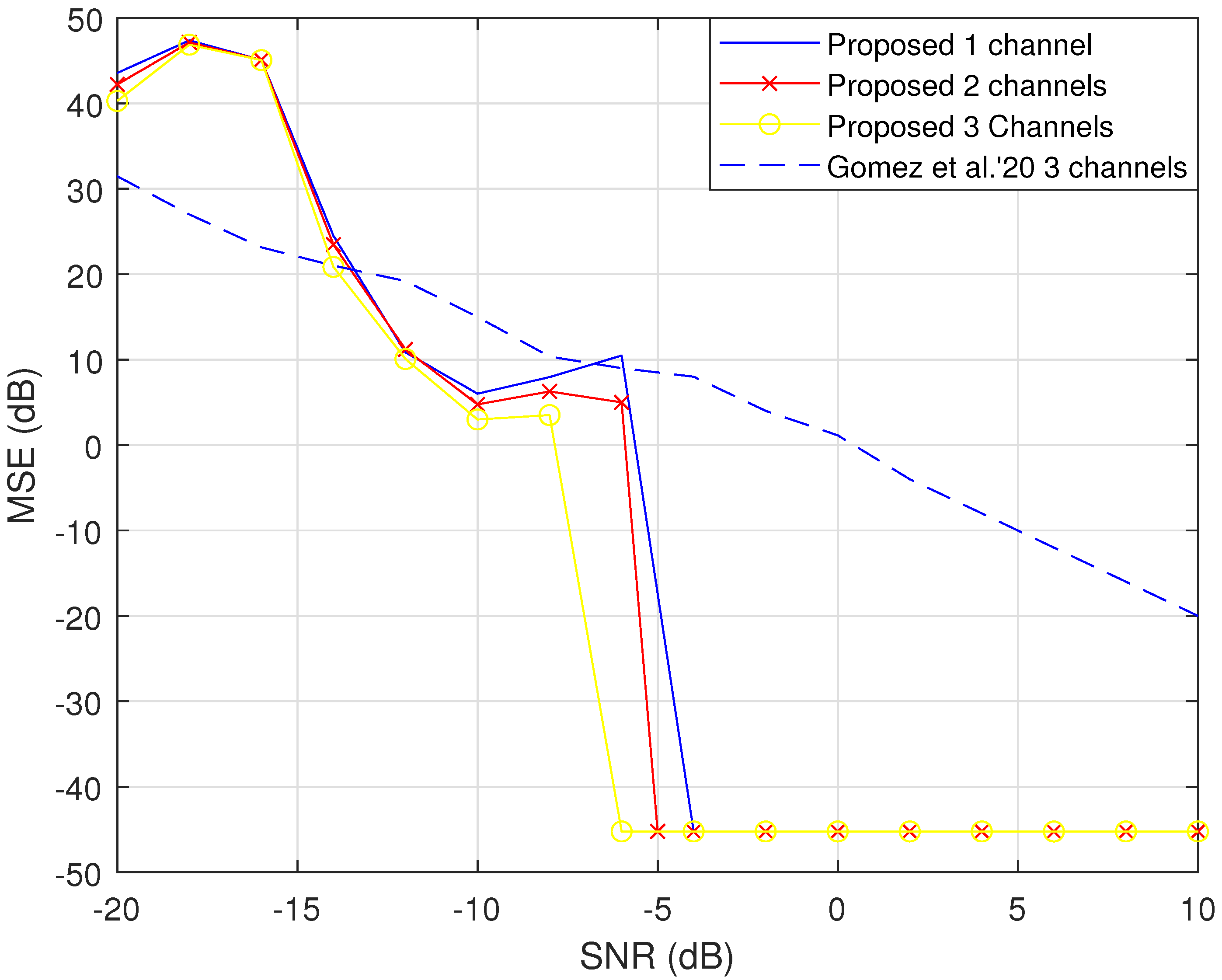
After showing the different variables of the algorithm, in Figure 11, the normalized mean squared error (MSE) is shown for different SNRs at the receiver. In these simulations, the target is located in different positions, as is the DVB-T transmitter (see Table 1 for more details). Although the target and receivers are placed in different positions, no trajectory is obtained, only coordinates are estimated. In this figure, the results of our proposal are shown. Additionally, as in [23], we present the use of several channels transmitted by the same DVB-T emitter in order to improve the results of channel estimation; up to three different channels, which is a common situation in most places, i.e., the reception of at least three channels properly is a setup typical of many applications. Several strategies have been tested, and that in the figures is the optimal approach, involving the coherent incorporation of equal gain combining the pilot signals of all different channels. On this basis, the SNR is improved, and the channel’s estimations are also improved. For comparison purposes, the algorithm proposed in [35] was also adapted to this scenario, and the results show that our proposal outperforms it. The SNR is an important variable to take into account in radar systems [36].

The normalized MSE is calculated as follows

$$MSE={\displaystyle \frac{1}{N}}\sum _{n=1}^N\sqrt{{\left({\displaystyle \frac{\mathbf{x}-{\widehat{\mathbf{x}}}_{\mathbf{n}}}{\mathbf{x}}}\right)}^2}$$

(17)

where N is the total number of simulated samples.

As can be seen in Figure 11, the estimation for lower values of SNR is poor. However, once the estimates are within what we could define as the lock-in range of the algorithm, the error is very small because the algorithm will provide a position that is very close to the true value. This lock-in range is the SNR range that allows the estimation of coordinates within a level of accuracy that ensures that the iterative algorithm is able to correct almost completely. The lock-in range is able to support large errors of dozens of meters in estimations. Moreover, since we rely solely on channel estimation to determine the time of arrival, and thus the distance, the crucial factor is the delay of the taps, rather than their amplitude. These two aspects enhance the robustness of our proposal, ensuring good performance even when the receiver has a low SNR.

In Figure 11, we present curves for using two and three different channels simultaneously. As shown, the benefits of using several channels are a couple of dB in the working range. For comparison purposes, the proposal in [35] (which we adapted to this scenario) is included in the figure. Since the proposal in [35] deals with the estimation of the trajectory using several (up to six) different transmitters and applying the Kalman filter to the signal received from the different transmitters, we made the following modifications to adapt it to our scenario. First, a single transmitter is used; however, we utilize three different signals coming from the three frequency channels used by the transmitter, i.e., we have three signals from the transmitter. Moreover, we do not estimate speed, and the simulation has a short enough duration to guarantee that the target may be considered static. It is clear that our proposal outperforms the alternative once the SNR is higher than −6 dB.

5. Conclusions

In this paper, a novel approach to target coordinate estimation is proposed and analyzed. The traditional LS formula for estimating positioning is robust when there are several widely separated receivers, as the errors are relatively small compared to the differences in distances. However, this traditional method is highly sensitive to errors when using a single receiver with multiple antennas. Moreover, a single-location compact PR is more convenient than its more widely distributed form. Thus, by leveraging the weakness of the formula when the antennas are co-located in a single receiver, the formula is adapted, resulting in an iterative algorithm for refining the initial estimations. After checking and validating the algorithm through simulations, we can conclude that it is a simple yet effective solution to the estimation of target coordinates, even in a low SNR environment. For further research, the algorithm is going to implement into a simple prototype based on universal software radio peripheral (USRP) B210 from Ettus and Matlab to validate the results.