Signal Super Prediction and Rock Burst Precursor Recognition Framework Based on Guided Diffusion Model with Transformer

Abstract

Implementing precise and advanced early warning systems for rock bursts is a crucial approach to maintaining safety during coal mining operations. At present, FEMR data play a key role in monitoring and providing early warnings for rock bursts. Nevertheless, conventional early warning systems are associated with certain limitations, such as a short early warning time and low accuracy of early warning. To enhance the timeliness of early warnings and bolster the safety of coal mines, a novel early warning model has been developed. In this paper, we present a framework for predicting the FEMR signal in deep future and recognizing the rock burst precursor. The framework involves two models, a guided diffusion model with a transformer for FEMR signal super prediction and an auxiliary model for recognizing the rock burst precursor. The framework was applied to the Buertai database, which was recognized as having a rock burst risk. The results demonstrate that the framework can predict 360 h (15 days) of FEMR signal using only 12 h of known signal. If the duration of known data is compressed by adjusting the CWT window length, it becomes possible to predict data over longer future time spans. Additionally, it achieved a maximum recognition accuracy of 98.07%, which realizes the super prediction of rock burst disaster. These characteristics make our framework an attractive approach for rock burst predicting and early warning.

1. Introduction

Rock burst, a major hazard in coal mining, frequently results in significant casualties and property damage. Investigating risk indicators prior to rock burst events is essential for forecasting such disasters in mining operations; some scholars have studied the current status of coal and gas outburst risk identification in underground coal mines, analyzed the challenges and limitations of existing methods, and proposed directions for future research [1,2,3]. Therefore, it is critical that we use a method to accurately obtain the precursor characteristics of rock burst as soon as possible. To accurately forecast rock burst disasters, numerous monitoring and early warning techniques have been developed, achieving significant advancements, including the fracture-induced electromagnetic radiation (FEMR) monitoring method, which are generally applied in the field of rock burst disaster early warning [4,5]. Researchers have investigated the formation mechanisms and transmission properties of FEMR signals; some scholars have provided insights into the activity of the Dead Sea transition zone by studying electromagnetic radiation signals from rock fractures before and after earthquakes in the Syrian–Turkish border area. Others have explored the electromagnetic radiation characteristics of rock fractures near the seismically active area in southern Israel [6,7,8]. Furthermore, numerous studies have explored the time–frequency domain features relevant to rock burst FEMR monitoring and early warning. Some scholars have proposed an early warning method based on microseismic monitoring for rockburst monitoring in Qinling water tunnels. In addition, some scholars have studied the improved waveform adaptive threshold method for microseismic signal denoising [9,10,11]. Thus, the FEMR monitoring process offers convenience, ensures continuity in monitoring data, and demonstrates efficacy in responding to rock burst precursory information and early warnings. However, the workload associated with manual procedures for analyzing rock burst precursor characteristics within FEMR signals is substantial, leading to an insufficient advance in warning time and inadequate accuracy in the recognition of precursor characteristics [12,13].

The enhancement in computational power has led to remarkable advancements in diverse deep-learning model algorithms and applications. These developments have enabled breakthroughs in areas such as computer vision, time-series data analysis, and beyond [14,15,16,17,18]. In the domain of geophysical studies, advanced machine-learning methodologies, particularly convolutional neural networks (CNNs) and recurrent neural networks (RNNs), have been utilized across various geophysical methods, which can not only realize recognizing the precursor characteristics of rock burst, but also predict the risk coefficient of disasters [19,20,21]. However, in the above method, the timing advance for early warning through precursor characteristics recognition is limited, generally only within about 7 days in advance. Some scholars have proposed a rock burst precursor electromagnetic radiation signal recognition and early warning method based on recursive neural network (RNN). Simultaneously, if the precursor characteristics signal lasts too long, it can result in delayed warning [5,22]. Hence, some scholars have opted for an alternative methodology, and used the RNNs and the transformer architecture to realize the disaster early warning in the type of time-series prediction. The time-series prediction method can predict FEMR signal data about 7 days in future, achieving the signal prediction in the short-term future. Some scholars have proposed a meteorological early warning method based on deep neural networks for predicting landslides caused by precipitation [23,24,25]. However, to achieve the high level of signal prediction accuracy, this method necessitates the integration of multi-variable data through multi-source fusion training, demanding an extensive array of sensor types deployed onsite. Simultaneously, each prediction for the short-term future requires a substantial volume of pre-existing data, imposing significant storage demands on coal mine databases, which is a challenge for many coal mines to meet. Some scholars have proposed a method for predicting the occurrence patterns of coal mine gas based on multi-source data fusion [26,27]. Given these constraints, there is a pressing need for a rock burst early warning method capable of predicting an FEMR signal in the deep future with minimal reliance on known univariate signal data and recognizing precursor characteristics.

Generative adversarial networks (GANs) consist of two parts: a generator that produces new data from random noise, and a discriminator that evaluates the generated samples against real data. These networks are trained simultaneously to achieve a Nash equilibrium, where neither network can improve its performance without the other adjusting its approach. GANs are recognized as an unsupervised learning technique capable of generating new data that align with the distribution of the training dataset [28,29,30,31,32]. Some scholars have proposed guided learning methods to improve the training process of GANs. Guided generative adversarial networks (GGANs), an advanced variant of GANs, enable controlled data generation by incorporating auxiliary information like labels. These networks have shown enhanced performance over prediction-based models, particularly when applied to unseen data with limited training samples [33,34,35,36]. These networks have been used to solve the spectrogram out-painting task, and predict the loss time-frequency data, which have the ability to predict the missing data [37,38,39]. While GAN-based architectures present numerous advantages compared to predictive models, including their proficiency in generalizing predictions across smaller and varied datasets and their aptitude for capturing complex conditional distributions, they are not devoid of limitations. A significant concern is the phenomenon of “mode collapse”, wherein the generator yields outputs with restricted diversity, thereby inadequately reflecting the full spectrum of variability inherent in the training data. This issue can hinder the model’s ability to generate realistic and diverse samples, ultimately impacting its effectiveness in applications requiring high variability and fidelity [33,34,40]. Moreover, these networks may encounter the challenge of “non-convergence”, where the learning process fails to achieve a Nash equilibrium, leading to unstable performance. To address these shortcomings of GANs, diffusion-based models have been introduced as an alternative approach [41,42].

To overcome the constraints inherent in GANs, diffusion models have been introduced. These models systematically incorporate Gaussian noise into the training samples until they are fully transformed into pure noise. This process enables the neural network to gradually eliminate noise and extract valuable insights from the data [43,44,45]. Recently, guided diffusion models have demonstrated remarkable prowess in tasks involving pixel matrix data predictions [46,47,48]. Notably, they have been successfully applied in generating pixel matrix data from textual descriptions, achieving pixel matrix data resolution and inpainting, and facilitating pixel-to-pixel convert, and pixel matrix data out-painting [49,50,51]. This underscores the extraordinary potential of diffusion-based models to enhance the accuracy of FEMR signal prediction in the deep future.

The guided diffusion model provides new ideas for signal prediction tasks [52,53,54,55]. This study converts the FEMR signal time-series data into corresponding time–frequency data through Fourier transform, and uses the guided diffusion model to predict the FEMR signal time-frequency data in the deep future based on known data. In order to achieve FEMR signal prediction in the deep future, we added the recurrent structure in the guided diffusion model in the super prediction process. However, diffusion models, which focus on predicting the incremental noise introduced during each iteration, face challenges when a fixed amount of noise is applied uniformly across the dataset. This can cause some samples to degrade more rapidly than others, introducing instability during training and resulting in errors in the predicted data outcomes [56,57,58,59]. Furthermore, if it involves the continuous generation of signal data in the deep future based on partially known data, the error of each generation and the prediction result of the model will accumulate in the data prediction process, which is fatal for deep future data prediction tasks [60,61,62,63]. This requires using a method to restore the data predicted in each recurrence by the guided diffusion model to ensure that it provides accurate known data for the next recurrence.

Over the past five years, deep learning is witnessing a remarkable revival, largely fueled by the emergence and widespread adoption of transformer-based architectures [64,65,66,67]. The transformer-based methods have shown impressive performance in pixel matrix data restoration tasks, such as pixel matrix data super-resolution. This study added a transformer-based data restoration architecture in the prediction process, which can restore the missing pixels in the predicted data, and provide higher quality known data for the next recurrence in the prediction process. To conclude, the transformer-based data restoration architecture significantly contributes to the efficacy of guided diffusion models in predicting deep-future FEMR signal time–frequency data, which can realize the FEMR signal super prediction.

This study introduces a novel guided diffusion model with a transformer-based framework that can predict the FEMR signal in the deep future through a minimal amount of known FEMR signal and an auxiliary model to recognize rock burst precursor characteristics. Our methodology consists of a two-stage process, as illustrated in Figure 1, which outlines the framework’s schematic. Initially, we employ a guided diffusion model integrated with a transformer to forecast FEMR signals over an extended future period. Subsequently, a transformer-based auxiliary model is utilized to identify the precursor characteristics of rock bursts within the FEMR signals. This approach enables the prediction of FEMR signals up to 360 h (15 days) into the future using only 12 h of known signal data. As a result, the time advance for rock burst early warning, as well as the precision of precursor characteristic identification, have been significantly enhanced.

2. Methodology

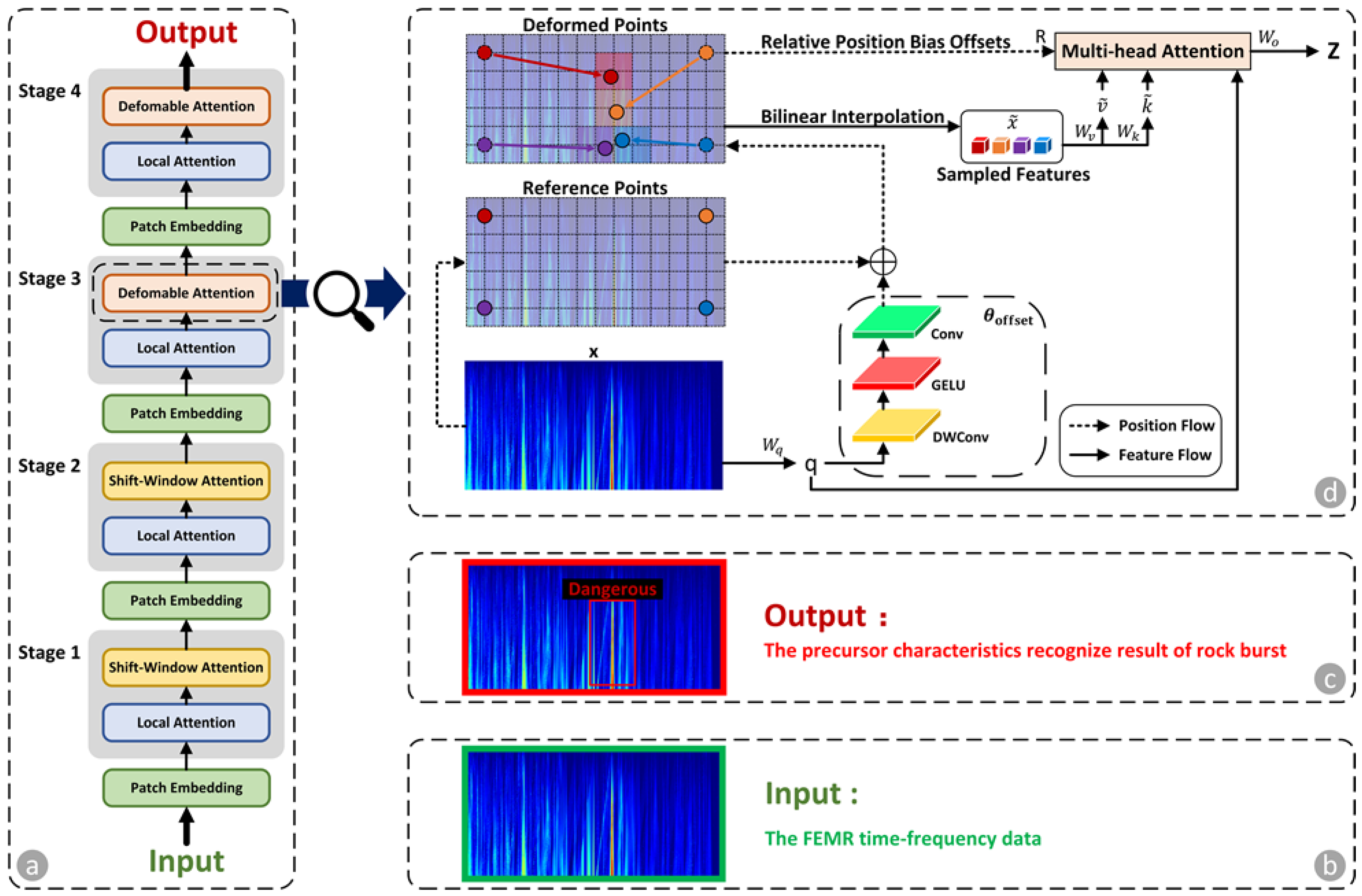
2.1. Auxiliary Model

The guided diffusion model with transformer can predict the FEMR signal data in deep future. To achieve effective early warning of rock bursts, it is essential that we identify precursor characteristics within FEMR time–frequency data. Transformers, which rely on self-attention mechanisms, have gained widespread popularity in natural language processing tasks. Recently, there has been a rising focus in adapting transformer-based methods to a variety of computer vision applications [67,68,69,70]. In our study, we employ a transformer-based architecture as the core model for identifying precursor characteristics of rock bursts.

Figure 2 illustrates the schematic of the auxiliary model designed to identify precursor characteristics of rock bursts in FEMR time–frequency data. The input data, which consist of summarized FEMR time–frequency data predicted by the guided diffusion model with transformer, is initially processed using a non-overlapping convolution to generate patch embeddings, followed by a normalization layer. The auxiliary model comprises four stages: The first two stages focus on learning local characteristics through attention mechanisms. In the third and fourth stages, the FEMR time–frequency characteristic maps are first processed by a window local attention mechanism to aggregate local information, and then passed through a deformable attention block to model global relationships between the locally enhanced tokens. The output of the auxiliary model provides the recognized precursor characteristics of rock bursts, with “Dangerous” indicators marked by red boxes.

Deformable attention block, as illustrated in Figure 2d, is the key to recognizing the precursor characteristics of rock burst. Given the input characteristics map $x$ of FEMR time–frequency data, a uniform grid of points is generated as the references. To determine the displacement for each reference location, as shown in Equation (1), the feature maps are linearly mapped to the query tokens $q=x{W}_q$, as shown in Equation (2), and then directed into a compact sub-network ${\theta }_{offset}\left(·\right)$ to output the offsets $\Delta p={\theta }_{offset}\left(q\right).$ Subsequently, the features are extracted at the positions of the deformed points to serve as keys and values, followed by the application of projection matrices:

$$q=x{W}_q, \tilde{k}=\tilde{x}{W}_k, \tilde{v}=\tilde{x}{W}_v,$$

(1)

$$\mathsf{\Delta }p={\theta }_{o\mathrm{f}\mathrm{f}\mathrm{s}\mathrm{e}\mathrm{t}}\left(q\right), \tilde{x}=\varnothing \left(x;p+∆p\right).$$

(2)

where $q$, $\tilde{k}$, and $\tilde{v}$ denote query, deformed key, and deformed value embeddings, respectively. $W_q$, $W_k$, $W_v$ are matrices.

Specifically, as shown in Equation (3), we set the sampling function $\mathrm{\varnothing }\left(·;·\right)$ to a bilinear interpolation process to ensure differentiability:

$$\varnothing \left(z;\left(p_x,p_y\right)\right)=\sum _{\left(r_x,r_y\right)}g\left(p_x,r_x\right)g\left(p_y,r_y\right)z\left[r_y,r_x,:\right]$$

(3)

where $g\left(a,b\right)=max(0, 1-|a-b\left|\right)$ and $\left(r_x,r_y\right)$ indexes all the locations on $z$. Since it is non-zero exclusively at the four nearest integral points to $g$, it reduces Equation (3) to a weighted average across these four positions.

Following established methodologies, as shown in Equation (4), we apply multi-head attention to $q,k,v$ and incorporate relative positional offsets $R$. The output of a single attention head is expressed as follows:

$$z^{\left(m\right)}=\sigma \left(q^{\left(m\right)}{\tilde{k}}^{{\left(m\right)}^{⊺}}/\sqrt{d}+\varphi \left(\widehat{B};R\right)\right){\tilde{v}}^{\left(m\right)}$$

(4)

where $\sigma (·)$ represents the softmax function, and $d=C/M$ indicates the dimensionality of each head. $z^{\left(m\right)}$ refers to the embedding output generated by the m-th attention head. $\varphi \left(\widehat{B};R\right)$ are derived from the position embedding, following established methodologies but with specific modifications.

The features from each head are combined through $W_o$ concatenation and then transformed to produce the final output $z$, as described in Equation (5).

$$z=Concat\left(z^{\left(1\right)},\dots ,z^{\left(M\right)}\right)W_o$$

(5)

where $W_o$ are the projection matrices.

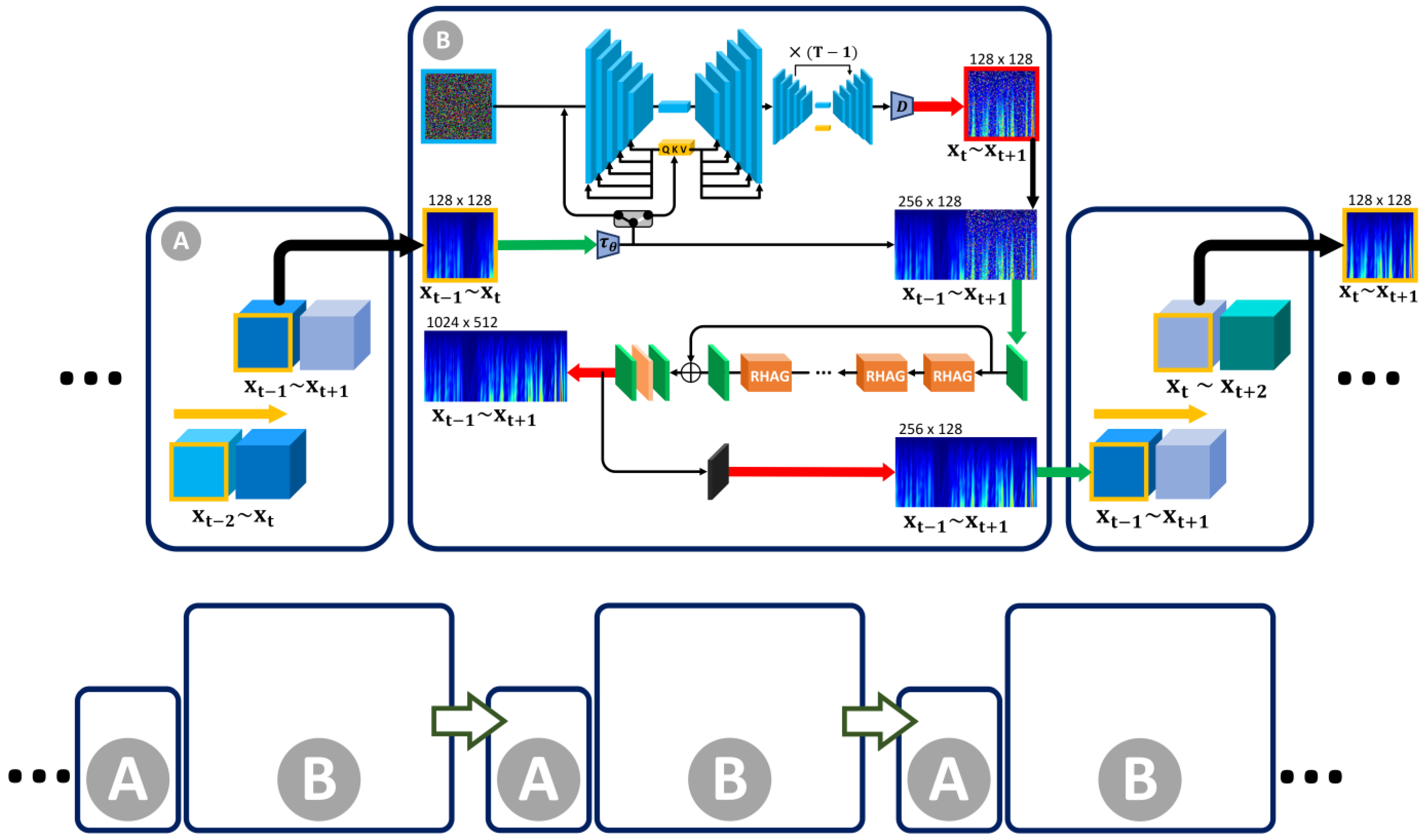
2.2. Guided Diffusion Model with Transformer

To achieve FEMR signal super prediction, the guided diffusion model with transformer can predict the signal in deep future. In the recurrence structure of the guided diffusion model with transformer, each 12 h future can be predicted through the data from previous 12 h. In order to obtain high-quality future FEMR signal time–frequency data in each recurrence of prediction tasks, we added a transformer-based data restoration architecture in guided diffusion model to restore the missing pixels in predicted FEMR signal data.

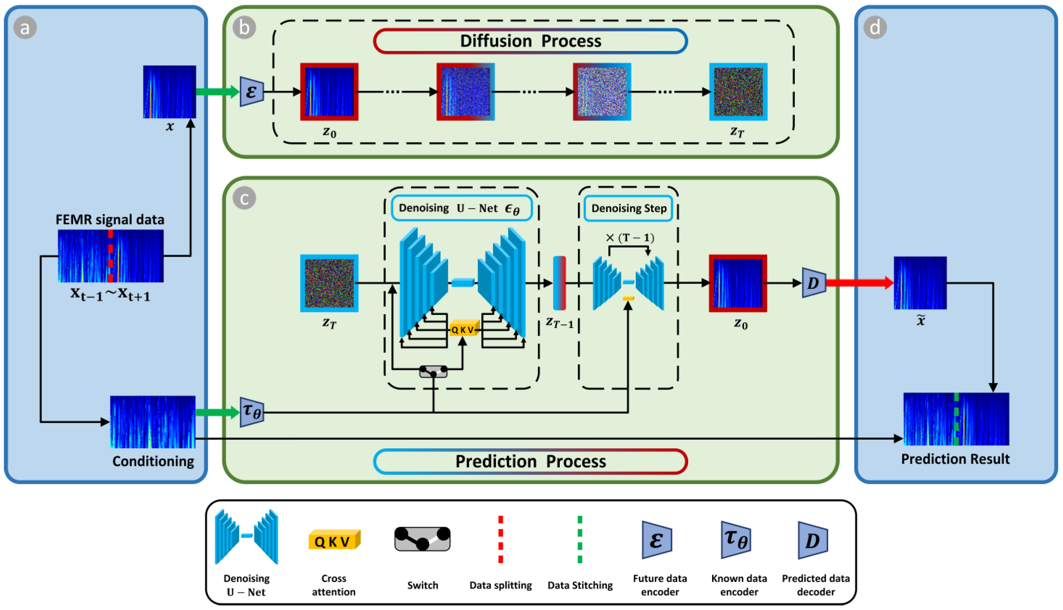
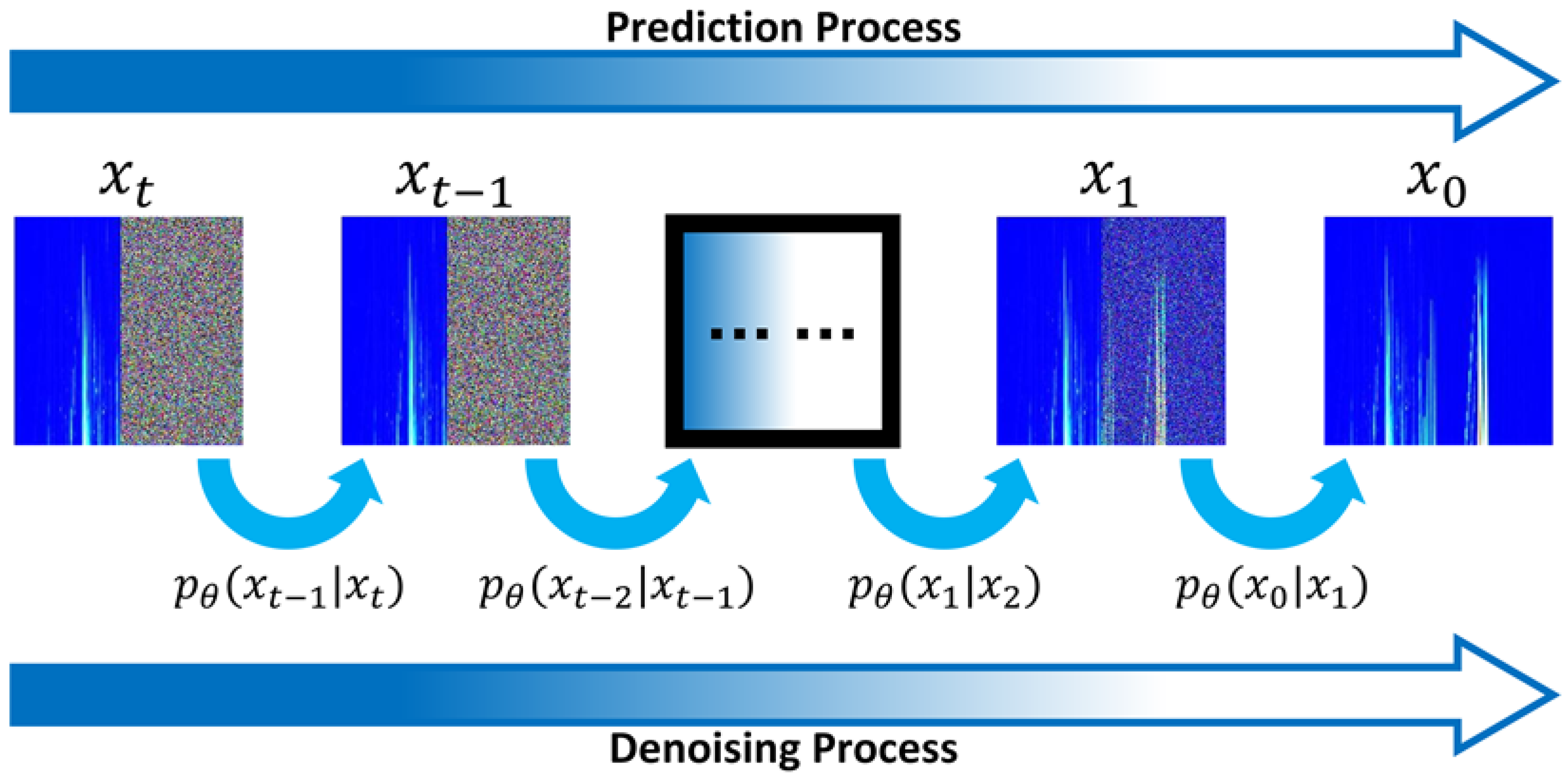
2.2.1. Guided Diffusion Model

Diffusion models are probabilistic frameworks that seek to model data distribution by iteratively refine a variable initialized with a normal distribution through a denoising process. This process involves establishing a Markov chain of diffusion steps, where systematic noise is gradually introduced to the input data during the forward diffusion process [71]. Considering the future time–frequency data as input $z_0$, as shown in Equations (6) and (7), the forward diffusion process can be represented as a Markov chain with a length of $T$:

$$q(z_t\left|z_{t-1}\right):=N\left(z_t;\sqrt{1-{\beta }_t}{z}_{t-1},{\beta }_t{\rm I}\right); {\beta }_t\in \left(\mathrm{0,1}\right);t\in \left\{1,\dots ,T\right\}$$

(6)

$$q(z_{1:T}\left|z_0\right):={\prod }_{t=1}^{T}q(z_t\left|z_{t-1}\right);t\in \left\{1,\dots ,T\right\}$$

(7)

where ${\beta }_t\in \left(\mathrm{0,1}\right)$ is the variance scheduler that regulates the step size of the noise added $t\in \left\{1,\dots ,T\right\}$ is the $t$ uniformly sampled from $\left\{1,\dots ,T\right\}$.

Our goal is to predict future time–frequency data from noise input $z_t\approx N(0,I)$ given a condition (known data), with the trained guided diffusion model consisting of future data encoder $\mathrm{ℇ}$, predicted data decoder $D$, and known data encoder ${\tau }_{\theta }$, which paves the way to controlling the prediction process via known data $y$. Given time–frequency data $x$, the encoder $\mathrm{ℇ}$ encodes $x$ into a latent representation $z=\mathrm{ℇ}\left(x\right)$, and the decoder $D$ reconstructs the time–frequency data from the latent, giving $\tilde{x}=D\left(z\right)=D\left(\mathrm{ℇ}\right(x\left)\right)$.

The data prediction can be achieved using a conditional denoising autoencoder ${ϵ}_{\theta }\left(z_t,t,{\tau }_{\theta }\left(y\right)\right)$, the conditional denoising autoencoder can predict the future time–frequency data given known data conditions. With a U-Net backbone and cross-attention mechanism, the guided diffusion model excels at learning attention-based models from known data. To pre-process known data $y$, we introduce an encoder ${\tau }_{\theta }$ that projects $y$ to an intermediate representation ${\tau }_{\theta }\left(y\right)\in R^{M\times d_{\tau }}$, which is then mapped to the intermediate layers of the U-Net through a cross-attention layer that implements the attention $\left(Q,K,V\right)=softmax\left({\displaystyle \frac{Q{K}^T}{\sqrt{d}}}\right)·V$, with $Q=W_Q^{\left(i\right)}·{\phi }_i\left(z_t\right)$, $K=W_K^{\left(i\right)}·{\tau }_{\theta }\left(y\right)$, and $V=W_V^{\left(i\right)}·{\tau }_{\theta }\left(y\right)$. Here, ${\phi }_i\left(z_t\right)\in R^{N\times d_{ϵ}^i}$ denotes a (flattened) intermediate representation of the U-Net, which is used for implementing ${ϵ}_{\theta }$, and $W_V^{\left(i\right)}\in R^{d\times d_{ϵ}^i}$, $W_Q^{\left(i\right)}\in R^{d\times d_{\tau }}\&W_K^{\left(i\right)}\in R^{d\times d_{\tau }}$ are learnable projection matrices. See Figure 3 for a visual depiction. Based on known data-conditioning pairs, as shown in Equation (8), we subsequently learn the conditional $L_{SDM}$ via:

$$L_{SDM}≔{{\rm E}}_{ℇ\left(x\right),y, ϵ~{\rm N}\left(\mathrm{0,1}\right), t)}\left[{‖ϵ-{ϵ}_{\theta }\left(z_t, t,{\tau }_{\theta }\left(y\right)\right)‖}_2^2\right];t\in \left\{1,\dots ,T\right\}$$

(8)

where both ${\tau }_{\theta }$ and ${ϵ}_{\theta }$ are jointly optimized via Equation (8).

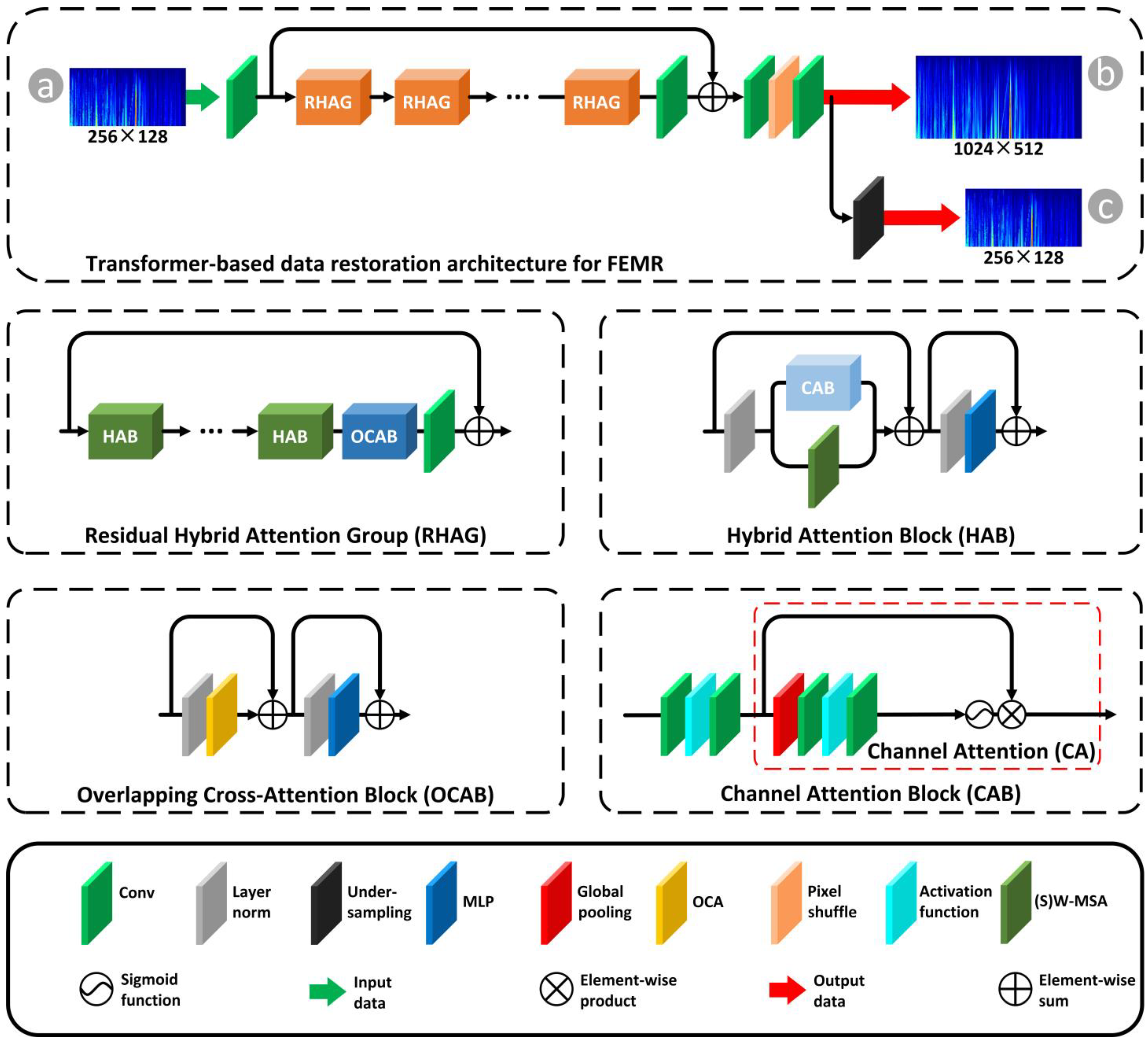
2.2.2. Transformer-Based Data Restoration Architecture

As shown in Figure 4, to acquire high-quality future FEMR signal time–frequency data in each iteration of prediction tasks, we integrated a transformer-based data restoration architecture within the guided diffusion model. This addition is specifically designed to restore the missing pixels in the predicted FEMR signal data.

The transformer-based data restoration architecture adopts a residual in residual (RIR) structure, comprising three key components: shallow feature extraction, deep feature extraction, and image reconstruction. The shallow characteristics extraction part uses a $3\times 3$ convolution layer to extract shallow characteristics from the low-quality input image as Equation (9):

$$F_0=H_{SF}\left(I_{LQ}\right)$$

(9)

where $F_0$ is the shallow characteristics and $I_{LQ}$ is low-quality (LQ) input image.

The deep characteristics extraction part utilizes a residual hybrid attention group (RHAG) to process intermediate characteristics and a final $3\times 3$ convolution layer to aggregate information as Equation (10):

$$F_{DF}=H_{DF}\left(F_0\right)$$

(10)

where $H_{DF}$ consists of RHAG and one $3\times 3$ convolution layer.

The image reconstruction part combines shallow and deep characteristics and reconstructs the high-quality (HQ) image using a reconstruction module with pixel-shuffle for super-resolution tasks or two convolutions for same-resolution tasks as Equation (11):

$$I_{HQ}=H_{Rec}\left(F_0+F_{DF}\right)$$

(11)

where $H_{Rec}(·)$ denotes the reconstruction module.

The residual hybrid attention group (RHAG) comprises two main components: hybrid attention blocks (HAB) and overlapping cross-attention blocks (OCAB). The HAB module integrates self-attention and channel attention mechanisms, enabling the activation of a broader range of input pixels and boosting reconstruction performance. It employs a large window size for window-based self-attention and incorporates a channel attention block (CAB) to dynamically adjust feature scaling. On the other hand, the OCAB module improves cross-window interactions by applying overlapping windows to key and value features, ensuring that the query can access richer contextual information. Figure 4 shows transformer-based data restoration architecture specifically.

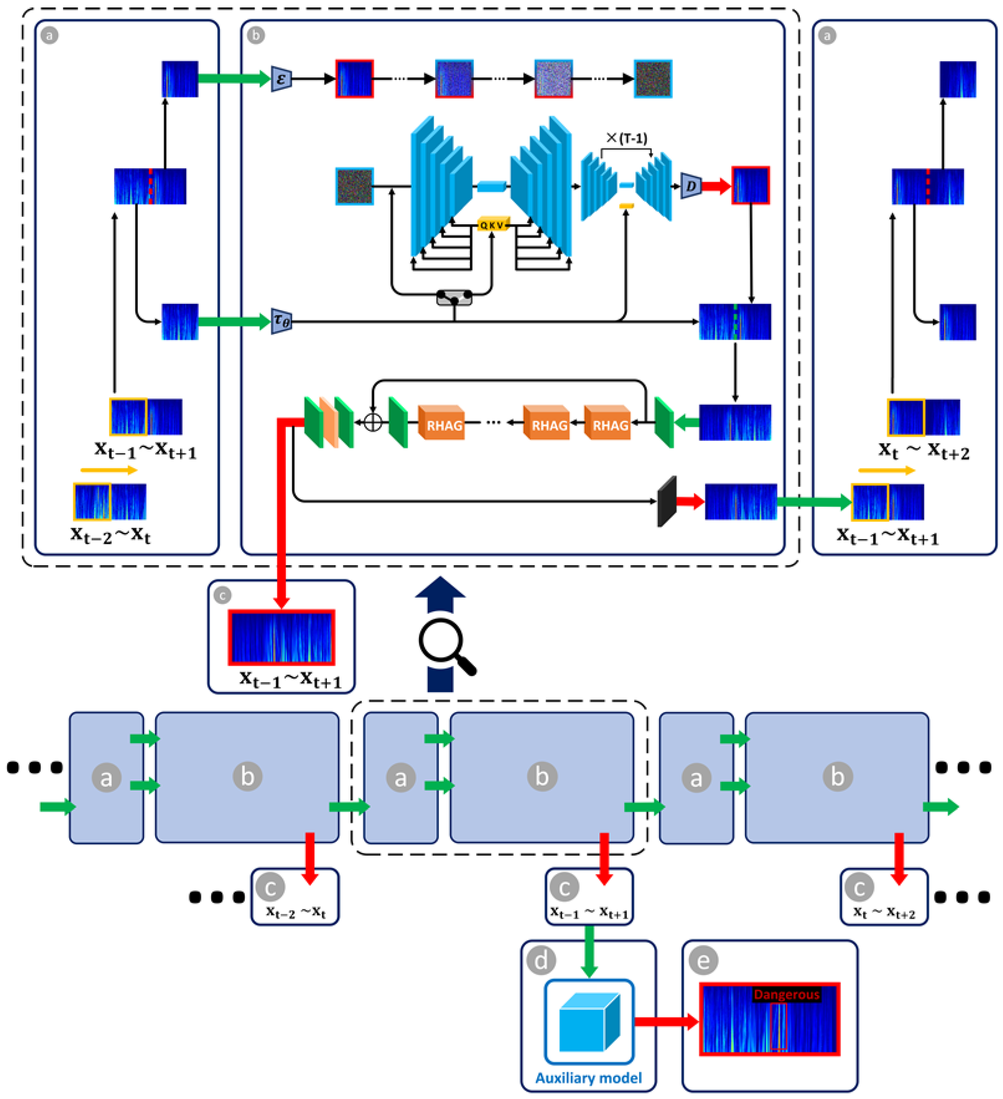
2.2.3. Recurrent Structure for Super Prediction

In this study, as shown in Figure 5, the super prediction approach refers to the use of recurrent structure to achieve multi-step prediction of precursor signals for rock outburst. This method not only predicts the signal for the next time step but also recursively generates predictions for multiple future time steps, thus providing a longer warning horizon.

The recursive super prediction strategy is a key innovation in this study. We split the time–frequency data into segments of specific durations. During model training, we use the previous segment of data as input to predict the next segment. Then, we use the prediction results from the previous step serves as input for the next prediction. Through this recursive process, the model generates predictions for multiple future time steps. By introducing the recurrent structure, this study achieved super prediction of FEMR signals, significantly improving both prediction time span.

2.3. Dataset Preparation

2.3.1. Acquisition of FEMR Data

As shown in Figure 6, the FEMR data from the NO.6, NO.7, and NO.8 return wind roadway in the West No. 3 mining area of the Buertai coal mine from January 2019 to May 2023 were selected as the research subject.

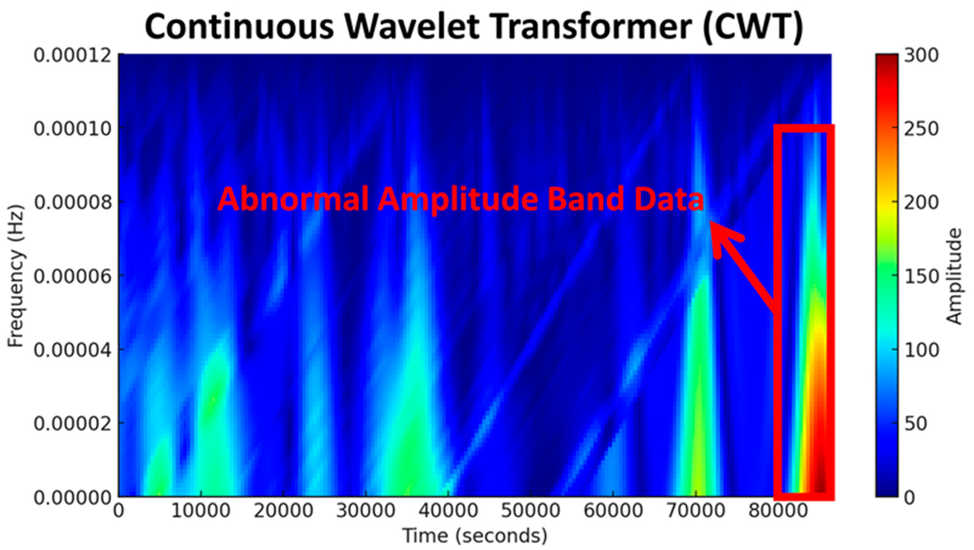
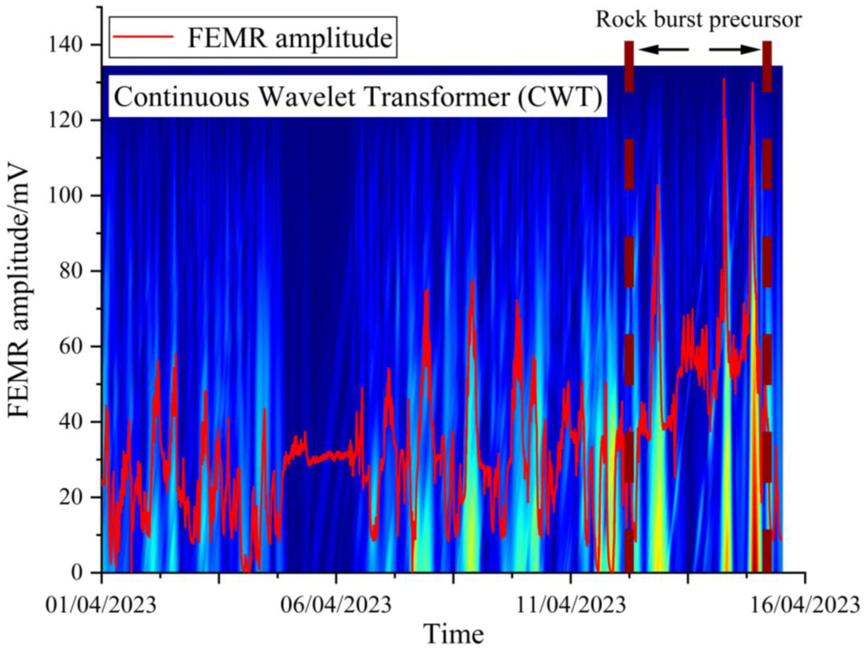
2.3.2. Principle of Continuous Wavelet Transform (CWT)

Wavelet transforms have become essential tools in various signal-processing fields, with the continuous wavelet transform (CWT) standing out for its effectiveness in signal analysis. In CWT, the wavelet associated with scale $a$ and time position $b$ is expressed as Equation (12):

$${\phi }_{a,b}\left(t\right)={\displaystyle \frac{1}{\sqrt{\left|a\right|}}}\phi \left({\displaystyle \frac{t-b}{a}}\right)$$

(12)

where $\phi \left(t\right)$ is the fundamental wavelet that acts as a ‘prototype’, serving as a bandpass filter. The factor ${\left|a\right|}^{-1/2}$ ensures energy preservation. The time-scale parameters (b, a) are discretized which can be approached in various ways, leading to different forms of wavelet transforms. Following the conventions of the classical Fourier transform, this research adopts a comparable framework. The concept of CWT was first introduced by Goupillaud. Both the time $\mathrm{t}$ and timescale parameters vary continuously as Equation (13):

$$CWT\left\{x\left(t\right);a,b\right\}=\int x\left(t\right){\phi }_{a,b}^{\mathrm{*}}\left(t\right)dt$$

(13)

In Equation (13), the asterisk denotes the complex conjugate operation, and the wavelet sequence (WS) coefficients correspond to the sampled continuous wavelet transform (CWT) coefficients. Time is modeled as a continuous variable, whereas the timescale parameters ($b$, $a$) are defined within the timescale plane ($b$, $a$).

To enhance data reliability and minimize errors or omissions during transmission, each time–frequency window contains 120 selectively sampled points. Furthermore, the implementation of overlapping data segments ensures seamless and continuous data analysis.

2.3.3. Time–Frequency Analysis of FEMR

The FEMR data were processed using CWT. Figure 7 shows the CWT data of FEMR signals with significant dynamic performance. The CWT analysis of FEMR data training samples in the database indicates that, in the abnormal state, the dominant amplitude band of the FEMR data is mainly concentrated between 80 to 230, as shown in Figure 7. The findings demonstrate that the time–frequency features of FEMR signals under normal conditions exhibit notable distinctions compared to those observed during abnormal conditions, enabling the detection of early warning signs preceding abrupt incidents.

Based on above analysis, we believe that the time–frequency characteristics of FEMR under normal conditions are significantly different from those in abnormal conditions, and can be used to recognize precursor characteristics of rock burst.

3. Results

3.1. Dataset Creation and Enhancement

The research focused on the Buertai coal mine in Erdos City, where uniform sensor models and standardized sampling procedures were implemented across all working faces. The investigation leveraged FEMR signal data spanning January 2019 through May 2023, extracted from the mine’s comprehensive database. Given the intermittent nature of rock burst precursor manifestations during extraction activities, the potential for model overfitting due to limited data samples was mitigated through strategic data expansion methodologies. These approaches were specifically designed to strengthen the predictive model’s resilience. To account for geographical variations in frequency distribution patterns that might affect precursor identification, the research team implemented advanced time–frequency characteristic enhancement strategies. These included the spatial transformation of graphical representations, selective image segmentation, and the incorporation of controlled Gaussian noise at varying intensities (0.05 and 0.005). Through these techniques, the repository of enhanced time–frequency diagrams was expanded to 2600 instances, substantially boosting the model’s detection accuracy.

The methodology incorporated a rigorous field data acquisition process coupled with meticulous data labeling, followed by the systematic partitioning of the dataset into distinct groups for model training, evaluation, and final assessment. Following established research conventions, the FEMR records from the Buertai mine were proportioned into training and validation cohorts at an 80:20 distribution. The comprehensive documentation of EMR signal classifications within the database, including specific numerical distributions for both training and validation groups, is presented in

Table 1. The number of rock burst precursor training and validation sets in Buertai coal mine database.

Dataset	Buertai Coal Mine Database
	Rock Burst Precursor
Train	2080
Test	520

.

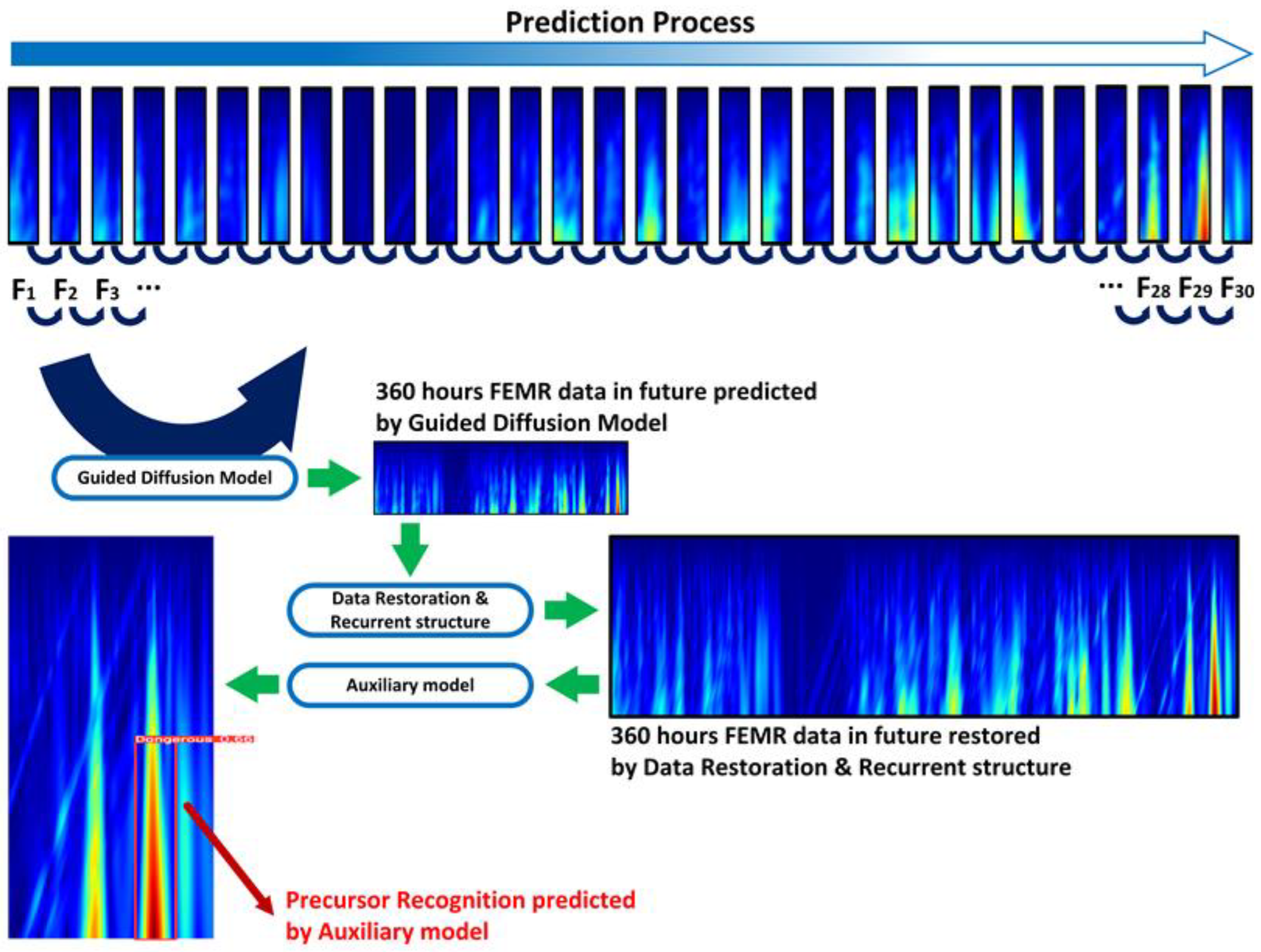
3.2. Signal Super Prediction and Precursor Recognition Framework Based on Guided Diffusion Model with Transformer

3.2.1. The Guided Diffusion Model

The guided diffusion model is primarily composed of a U-Net architecture, which includes an encoder, bottleneck, decoder, and output. The encoding component incorporates a feature extraction module based on convolutional operations with dimensions $3\times 6\times 64\times 64$, residual modules with dimensions $3\times 64\times 64\times 64, 3\times 128\times 32\times 32$, $3\times 256\times 16\times 16$, and $3\times 512\times 8\times 8$, down-sampling layers with dimensions $3\times 64\times 64\times 64$, $3\times 128\times 32\times 32$, and $3\times 256\times 16\times 16$, and an attention module with dimension $3\times 256\times 16\times 16$. The bottleneck includes residual modules with dimensions $3\times 512\times 8\times 8$ and an attention module with dimension $3\times 256\times 8\times 8$. The decoder comprises residual modules with dimensions $3\times 1024\times 8\times 8, 3\times 384\times 16\times 16, 3\times 192\times 32\times 32$ and $3\times 128\times 64\times 64$, as well as up-sampling layers with dimensions $3\times 256\times 8\times 8, 3\times 128\times 16\times 16$, and $3\times 64\times 32\times 32$. Finally, the output module is a convolutional layer with dimension $3\times 64\times 64\times 64$. The prediction steps of the guided diffusion model in the training set are shown in Figure 8.

The guided diffusion model’s parameter optimization was accomplished through the implementation of stochastic gradient descent (SGD) as the optimization algorithm. The training configuration employed a batch size of 8, while maintaining a dropout probability of 0.2 to mitigate the risk of overfitting. The learning rate was specifically tuned to $5\times {10}^{-5}$ for optimal convergence.

Throughout the training process, testing was performed every 10 epochs. Due to disk storage limitations, training was halted after 4 days and 13 h, reaching epoch 2428. The LOSS curve is a crucial tool for understanding the model’s training progress. Typically, during the early stages of training, the LOSS value is relatively high, as the model’s parameters are far from optimal. As training progresses, the model begins to adjust its weights and biases, leading to a decrease in the LOSS value. This downward trend reflects the model’s improvement in predicting the target outputs. Following a thorough evaluation of the loss values, the optimal model was saved at epoch 1850. The evaluation metrics, calculated through mean squared error (MSE) methodology for both training and validation datasets, demonstrated a consistent downward trajectory before reaching a plateau. This observed behavior suggests a successful convergence and the optimal adaptation of the Guided Diffusion architecture. The corresponding training loss progression is visually represented in Figure 9. All training procedures were executed on an RTX 5000 GPU equipped with 16 GB of VRAM (Nvidia, Santa Clara, CA, USA).

3.2.2. Transformer-Based Data Restoration and Recurrent Structure for Super Prediction

We use a transformer-based data restoration architecture to reconstruct the FEMR data predicted by the guided diffusion model. The recurrent structure can predict data for 360 h (15 days) in the future based on 12 h of FEMR data, due to the potential FEMR data missing during the recurrent prediction process. As shown in Figure 5, the Transformer-based data reconstruction architecture reads FEMR data with dimensions $256\times 128\times 1$, and the output FEMR data with dimensions $256\times 128\times 1$ and $1024\times 512\times 1$. FEMR data with dimensions $256\times 128\times 1$ are used for the next restoration, while FEMR data with dimensions $1024\times 512\times 1$ are used for rock burst precursor recognition. Based on the past 12 h of FEMR data, we achieved predictions for the next 360 h (15 days).

However, during the fourth prediction reconstruct, the data become challenging to restore, making it difficult to recognize precursor characteristics of rock burst. If the known data are compressed along the temporal dimension, it is theoretically possible to achieve predictions for a longer future time frame. All testing processes were completed on an RTX 5000 GPU with 16 GB of VRAM.

3.2.3. Auxiliary Model for Recognizing Rock Burst Precursor Characteristics

The input FEMR data for the auxiliary model has dimensions of $1024\times 512\times 3(\mathrm{H}\times \mathrm{W}\times \mathrm{C})$. Initially, the data are processed using a $4\times 4$ non-overlapping convolution with a stride of 4, followed by a normalization layer to generate ${\displaystyle \frac{H}{4}}\times {\displaystyle \frac{W}{4}}\times C$ patch embeddings. The architectural framework for building a multi-level feature hierarchy incorporates four distinct processing stages within its core structure, with each successive stage implementing incrementally larger stride values. Between consecutive stages, a non-overlapping $2\times 2$ convolution with a stride of 2 is applied to down-sample the characteristics map, reducing its spatial size by half and doubling the characteristics dimensions. For the classification task, the characteristics maps from the final stage are normalized, and a linear classifier with pooled characteristics is used to predict the logits.

In Stage 1, the number of blocks is 1, the channel dimension is 96, the region size in the local attention module is 7, and the number of heads in DMHA is 3. In Stage 2, the number of blocks is 1, the channel dimension is 192, the region size in the local attention module is 7, and the number of heads in DMHA is 6. In Stage 3, the number of blocks is 3, the channel dimension is 384, the region size in the local attention module is 7, the number of heads in DMHA is 12, and the offset groups in DMHA is 3. In Stage 4, the number of blocks is 1, the channel dimension is 768, the region size in the local attention module is 7, the number of heads in DMHA is 24, and the offset groups in DMHA is 6.

An auxiliary model, which has a depth of 225 layers and approximately $11\times {10}^6$ parameters, was used. The model’s parameter optimization was accomplished through the implementation of the stochastic gradient descent algorithm. The model was configured with a batch size of 3, a learning rate set at $1\times {10}^{-2}$, and a dropout rate of 0.9 to prevent overfitting. Throughout the training process, testing was conducted every epoch. Due to disk capacity constraints, the training was stopped after 55.2 min, at epoch 100. After the comprehensive verification of the loss value, the best training model was saved at epoch 57. The training metrics, calculated through binary cross-entropy (BCE) for both the training and validation datasets, displayed a consistent reduction before reaching equilibrium. This behavior confirms the successful convergence and optimal adaptation of the guided diffusion architecture. The corresponding training loss progression is illustrated in Figure 10. All training and testing processes were completed on an RTX 5000 GPU with 16 GB of VRAM. During the testing process, 510 out of 520 FEMR data samples were correctly recognized, resulting in an accuracy of 98.07%.

3.3. Early Warning Results for Rock Burst Using Signal Super Prediction and Precursor Recognition Framework

We selected 15 days of continuous FEMR data with rock burst risk, recorded from 1 April to 15 April 2023, from the No. 8 return wind roadway in the West No. 3 mining area of the Buertai coal mine, to test the framework. FEMR time-series data span from 00:00 on 1 April 2023, to 22:00 on 7 April 2023, during which the FEMR time-series data exhibit a periodic cyclic trend, indicating active mining operations at the working face. From 00:00 on 1 April 2023, to 15:51 on 9 April 2023, a slight cyclic growth trend in the FEMR time-series data can be observed. However, by 06:13 on 12 April 2023, the FEMR time-series data show a significant and pronounced cyclic growth trend, which can be identified as a distinctive signature preceding rock burst occurrences within the FEMR signal patterns.

We input the known FEMR data from 00:00 to 12:00 on 1 April 2023, into the super prediction framework to predict future data. The FEMR time-series data from April 1 to 15 April 2023 is shown in Figure 11, while the time-frequency data for the same period are presented in Figure 11. The results of the signal super prediction are shown in Figure 12, where we successfully predicted 360 h (15 days) of future FEMR data based on 12 h of known data. The prediction results demonstrate that the framework can achieve long-term data predicting using a relatively small amount of initial FEMR time-series data. We input the FEMR time-frequency data obtained from the framework’s super prediction results into an auxiliary model, which successfully recognized precursor characteristics of rock burst, and the confidence level for recognizing precursor characteristics is 0.66. The framework’s super prediction and precursor characteristics recognition results are shown in Figure 12. It can be observed that the precursor characteristics of FEMR exhibit a relatively high amplitude.

4. Conclusions

The traditional method of early warning through precursor recognition typically offers limited lead time, usually within 7 days. Prolonged precursor signals can delay warnings, posing challenges for timely intervention. Some researchers have utilized recurrent neural networks (RNNs) and transformer-based architectures for time-series prediction, achieving FEMR signal forecasting up to 7 days in advance. While effective for short-term predictions, this approach necessitates multi-source data fusion and extensive sensor deployments to ensure a high accuracy, relying on substantial pre-existing datasets. This requirement imposes significant storage burdens on coal mine databases, a persistent challenge in operational contexts.

In contrast, this study introduces an innovative approach leveraging a guided diffusion model coupled with a transformer-based data restoration architecture for the processing of known FEMR signals. This model facilitates the super prediction of FEMR data, forecasting up to 360 h (15 days) into the future based solely on 12 h of known data. Additionally, an auxiliary model is employed to identify rock burst precursor characteristics within the FEMR data. The empirical results underscore the efficacy of this approach in predicting FEMR signals over extended time periods, while also conducting a comprehensive analysis of the upward trends inherent in FEMR signals—key indicators of rock burst precursors.

The academic contribution of this method lies in its ability to extend prediction horizons and enhance the interpretability of rock burst precursor identification. With an accuracy rate of 98.07%, the approach significantly improves the reliability of early warning systems, advancing both the forecasting capability and risk assessment of rock burst hazards up to 15 days ahead. In conclusion, this study offers a novel and rigorous methodology that not only pushes the boundaries of prediction timelines but also contributes to the advancement of safety management and monitoring systems in coal mining operations, enhancing the accuracy and reliability of rock burst early warnings.

References

1. Zhang, G.; Wang, E. Risk identification for coal and gas outburst in underground coal mines: A critical review and future directions. Gas Sci. Eng. 2023, 118, 205106. [Google Scholar] [CrossRef]
2. Gu, S.; Zhang, W.; Jiang, B.; Hu, C. Case of rock burst danger and its prediction and prevention in tunneling and mining period at an irregular coal face. Geotech. Geol. Eng. 2019, 37, 2545–2564. [Google Scholar] [CrossRef]
3. Yin, S.; Wang, E.; Li, Z.; Zang, Z.; Liu, X.; Zhang, C.; Ding, X.; Aihemaiti, A. Multifractal and b-value nonlinear time-varying characteristics of acoustic emission for coal with different impact tendency. Measurement 2025, 248, 116896. [Google Scholar] [CrossRef]
4. Li, X.; Wang, E.; Li, Z.; Liu, Z.; Song, D.; Qiu, L. Rock burst monitoring by integrated microseismic and electromagnetic radiation methods. Rock Mech. Rock Eng. 2016, 49, 4393–4406. [Google Scholar] [CrossRef]
5. Di, Y.; Wang, E. Rock burst precursor electromagnetic radiation signal recognition method and early warning application based on recurrent neural networks. Rock Mech. Rock Eng. 2021, 54, 1449–1461. [Google Scholar] [CrossRef]
6. Das, S.; Frid, V.; Rabinovitch, A.; Bahat, D.; Kushnir, U. Insights into the Dead Sea Transform Activity through the study of fracture-induced electromagnetic radiation (FEMR) signals before the Syrian-Turkey earthquake (Mw-6.3) on 20.2.2023. Sci. Rep. 2024, 14, 4579. [Google Scholar] [CrossRef]
7. Bai, W.; Shu, L.; Sun, R.; Xu, J.; Silberschmidt, V.V.; Sugita, N. Mechanism of material removal in orthogonal cutting of cortical bone. J. Mech. Behav. Biomed. Mater. 2020, 104, 103618. [Google Scholar] [CrossRef]
8. Frid, V.; Rabinovitch, A.; Bahat, D.; Kushnir, U. Fracture electromagnetic radiation induced by a seismic active zone (in the Vicinity of Eilat City, Southern Israel). Remote Sens. 2023, 15, 3639. [Google Scholar] [CrossRef]
9. Wang, X.; Yu, S.; Yin, D. Time-frequency Characteristics of Micro-seismic Signals Before and after Rock Burst. In Proceedings of the 9th China-Russia Symposium “Coal in the 21st Century: Mining, Intelligent Equipment and Environment Protection” (COAL 2018), Qingdao, China, 18–21 October 2018; Atlantis Press: Amsterdam, The Netherlands, 2018; pp. 9–12. [Google Scholar]
10. Ma, T.; Lin, D.; Tang, L.; Li, L.; Tang, C.; Yadav, K.P.; Jin, W. Characteristics of rockburst and early warning of microseismic monitoring at qinling water tunnel. Geomat. Nat. Hazards Risk 2022, 13, 1366–1394. [Google Scholar] [CrossRef]
11. Zhang, Z.; Ye, Y.; Luo, B.; Chen, G.; Wu, M. Investigation of microseismic signal denoising using an improved wavelet adaptive thresholding method. Sci. Rep. 2022, 12, 22186. [Google Scholar] [CrossRef]
12. Wu, M.; Ye, Y.; Wang, Q.; Hu, N. Development of rockburst research: A comprehensive review. Appl. Sci. 2022, 12, 974. [Google Scholar] [CrossRef]
13. Zhang, S.; Tang, C.; Wang, Y.; Li, J.; Ma, T.; Wang, K. Review on early warning methods for rockbursts in tunnel engineering based on microseismic monitoring. Appl. Sci. 2021, 11, 10965. [Google Scholar] [CrossRef]
14. Voulodimos, A.; Doulamis, N.; Doulamis, A.; Protopapadakis, E. Deep learning for computer vision: A brief review. Comput. Intell. Neurosci. 2018, 2018, 7068349. [Google Scholar] [CrossRef]
15. Hewamalage, H.; Bergmeir, C.; Bandara, K. Recurrent neural networks for time series forecasting: Current status and future directions. Int. J. Forecast. 2021, 37, 388–427. [Google Scholar] [CrossRef]
16. Ahmed, S.; Nielsen, I.E.; Tripathi, A.; Siddiqui, S.; Ramachandran, R.P.; Rasool, G. Transformers in time-series analysis: A tutorial. Circuits Syst. Signal Process. 2023, 42, 7433–7466. [Google Scholar] [CrossRef]
17. Wang, Z.; She, Q.; Ward, T.E. Generative adversarial networks in computer vision: A survey and taxonomy. ACM Comput. Surv. (CSUR) 2021, 54, 1–38. [Google Scholar] [CrossRef]
18. Du, Z.; Liu, X.; Wang, J.; Jiang, G.; Meng, Z.; Jia, H.; Xie, H.; Zhou, X. Response characteristics of gas concentration level in mining process and intelligent recognition method based on bi-lstm. Min. Metall. Explor. 2023, 40, 807–818. [Google Scholar] [CrossRef]
19. Zhang, S.; Mu, C.; Feng, X.; Ma, K.; Guo, X.; Zhang, X. Intelligent dynamic warning method of rockburst risk and level based on recurrent neural network. Rock Mech. Rock Eng. 2024, 57, 3509–3529. [Google Scholar] [CrossRef]
20. Wojtecki, Ł.; Iwaszenko, S.; Apel, D.B.; Cichy, T. An attempt to use machine learning algorithms to estimate the rockburst hazard in underground excavations of hard coal mine. Energies 2021, 14, 6928. [Google Scholar] [CrossRef]
21. Mahmood, M.R.; Matin, M.A.; Sarigiannidis, P.; Goudos, S.K. A comprehensive review on artificial intelligence/machine learning algorithms for empowering the future IoT toward 6G era. IEEE Access 2022, 10, 87535–87562. [Google Scholar] [CrossRef]
22. Basnet, P.M.S.; Mahtab, S.; Jin, A. A comprehensive review of intelligent machine learning based predicting methods in long-term and short-term rock burst prediction. Tunn. Undergr. Space Technol. 2023, 142, 105434. [Google Scholar] [CrossRef]
23. Prasad, S.C.; Prasad, P. Deep recurrent neural networks for time series prediction. arXiv 2014, arXiv:1407.5949. [Google Scholar]
24. Huang, L.; Xiang, L. Method for meteorological early warning of precipitation-induced landslides based on deep neural network. Neural Process. Lett. 2018, 48, 1243–1260. [Google Scholar] [CrossRef]
25. Deb, S.; Chanda, A.K. Comparative analysis of contextual and context-free embeddings in disaster prediction from Twitter data. Mach. Learn. Appl. 2022, 7, 100253. [Google Scholar] [CrossRef]
26. Jiao, H.; Song, W.; Cao, P.; Jiao, D. Prediction method of coal mine gas occurrence law based on multi-source data fusion. Heliyon 2023, 9, e17117. [Google Scholar] [CrossRef]
27. Kiziroglou, M.E.; Boyle, D.E.; Yeatman, E.M.; Cilliers, J.J. Opportunities for sensing systems in mining. IEEE Trans. Ind. Inform. 2016, 13, 278–286. [Google Scholar] [CrossRef]
28. Liu, M.Y.; Tuzel, O. Coupled generative adversarial networks. In Advances in Neural Information Processing Systems; Curran Associates, Inc.: Newry, UK, 2016; Volume 29. [Google Scholar]
29. Adler, J.; Lunz, S. Banach wasserstein gan. In Advances in Neural Information Processing Systems; Curran Associates, Inc.: Newry, UK, 2018; Volume 31. [Google Scholar]
30. Brock, A. Large Scale GAN Training for High Fidelity Natural Image Synthesis. arXiv 2018, arXiv:1809.11096. [Google Scholar]
31. Zhang, H.; Goodfellow, I.; Metaxas, D.; Odena, A. Self-attention generative adversarial networks. In Proceedings of the International Conference on Machine Learning, PMLR, 2019, Long Beach, CA, USA, 9–15 June 2019; pp. 7354–7363. [Google Scholar]
32. Mirza, M. Conditional generative adversarial nets. arXiv 2014, arXiv:1411.1784. [Google Scholar]
33. Salimans, T.; Goodfellow, I.; Zaremba, W.; Cheung, V.; Radford, A.; Chen, X.; Chen, X. Improved techniques for training gans. In Advances in Neural Information Processing Systems; Curran Associates, Inc.: Newry, UK, 2016; Volume 29. [Google Scholar]
34. Radford, A. Unsupervised representation learning with deep convolutional generative adversarial networks. arXiv 2015, arXiv:1511.06434. [Google Scholar]
35. Nagpal, S.; Verma, S.; Gupta, S.; Aggarwal, S. A guided learning approach for generative adversarial networks. In Proceedings of the 2020 IEEE International Joint Conference on Neural Networks (IJCNN), Glasgow, UK, 19–24 July 2020; pp. 1–8. [Google Scholar]
36. Karras, T. A Style-Based Generator Architecture for Generative Adversarial Networks. arXiv 2019, arXiv:1812.04948. [Google Scholar]
37. Younesi, A.; Ansari, M.; Fazli, M.; Ejlali, A.; Shafique, M.; Henkel, J. A Comprehensive Survey of Convolutions in Deep Learning: Applications, Challenges, and Future Trends. IEEE Access 2024, 12, 41180–41218. [Google Scholar] [CrossRef]
38. Panariello, M. Low-Complexity Neural Networks for Robust Acoustic Scene Classification in Wearable Audio Devices; Politecnico di Torino: Turin, Italy, 2022. [Google Scholar]
39. Peng, J.; Liu, Y.; Wang, M.; Li, Y.; Li, H. Zero-Shot Self-Consistency Learning for Seismic Irregular Spatial Sampling Reconstruction. arXiv 2024, arXiv:2411.00911. [Google Scholar]
40. Goodfellow, I.; Pouget-Abadie, J.; Mirza, M.; Xu, B.; Warde-Farley, D.; Ozair, S.; Courville, A.; Bengio, Y. Generative adversarial nets. In Advances in Neural Information Processing Systems; Curran Associates, Inc.: Newry, UK, 2014; Volume 27. [Google Scholar]
41. Cao, H.; Tan, C.; Gao, Z.; Xu, Y.; Chen, G.; Heng, P.-A.; Li, S.Z. A survey on generative diffusion models. IEEE Trans. Knowl. Data Eng. 2024, 36, 2814–2830. [Google Scholar] [CrossRef]
42. Yang, L.; Zhang, Z.; Song, Y.; Hong, S.; Xu, R.; Zhao, Y.; Zhang, W.; Cui, B.; Yang, M.-H. Diffusion models: A comprehensive survey of methods and applications. ACM Comput. Surv. 2023, 56, 1–39. [Google Scholar] [CrossRef]
43. Dhariwal, P.; Nichol, A. Diffusion models beat gans on image synthesis. In Advances in Neural Information Processing Systems; Curran Associates, Inc.: Newry, UK, 2021; Volume 34, pp. 8780–8794. [Google Scholar]
44. Srivastava, A.; Sutton, C. Autoencoding variational inference for topic models. arXiv 2017, arXiv:1703.01488. [Google Scholar]
45. Ramesh, A.; Pavlov, M.; Goh, G.; Gray, S.; Voss, C.; Radford, A.; Chen, M.; Sutskever, I. Zero-shot text-to-image generation. In Proceedings of the International Conference on Machine Learning, PMLR, Virtual, 18–24 July 2021; pp. 8821–8831. [Google Scholar]
46. Zhu, L.; Zheng, Y.; Zhang, Y.; Wang, X.; Wang, L.; Huang, H. Temporal Residual Guided Diffusion Framework for Event-Driven Video Reconstruction. In Proceedings of the European Conference on Computer Vision; Springer: Cham, Switzerland, 2025; pp. 411–427. [Google Scholar]
47. Huang, Y.; Huang, J.; Liu, Y.; Yan, M.; Lv, J.; Liu, J.; Xiong, W.; Zhang, H.; Chen, S.; Cao, L. Diffusion model-based image editing: A survey. arXiv 2024, arXiv:2402.17525. [Google Scholar] [CrossRef] [PubMed]
48. Fuest, M.; Ma, P.; Gui, M.; Schusterbauer, J.; Hu, V.T.; Ommer, B. Diffusion models and representation learning: A survey. arXiv 2024, arXiv:2407.00783. [Google Scholar]
49. Blattmann, A.; Rombach, R.; Ling, H.; Dockhorn, T.; Kim, S.W.; Fidler, S.; Kreis, K. Align your latents: High-resolution video synthesis with latent diffusion models. In Proceedings of the IEEE/CVF Conference on Computer Vision and Pattern Recognition, Vancouver, BC, Canada, 18–22 June 2023; pp. 22563–22575. [Google Scholar]
50. Saharia, C.; Chan, W.; Chang, H.; Lee, C.; Ho, J.; Salimans, T.; Fleet, D.; Norouzi, M. Palette: Image-to-image diffusion models. In Proceedings of the ACM SIGGRAPH 2022 Conference Proceedings, Vancouver, BC, Canada, 7–11 August 2022; pp. 1–10. [Google Scholar]
51. Yu, J.; Lin, Z.; Yang, J.; Shen, X.; Lu, X.; Huang, T.S. Generative image inpainting with contextual attention. In Proceedings of the IEEE Conference on Computer Vision and Pattern Recognition, Salt Lake City, UT, USA, 18–23 June 2018; pp. 5505–5514. [Google Scholar]
52. Rombach, R.; Blattmann, A.; Lorenz, D.; Esser, P.; Ommer, B. High-resolution image synthesis with latent diffusion models. In Proceedings of the IEEE/CVF Conference on Computer Vision and Pattern Recognition, New Orleans, LA, USA, 19–20 June 2022; pp. 10684–10695. [Google Scholar]
53. Avrahami, O.; Fried, O.; Lischinski, D. Blended latent diffusion. ACM Trans. Graph. (TOG) 2023, 42, 1–11. [Google Scholar] [CrossRef]
54. Lovelace, J.; Kishore, V.; Wan, C.; Shekhtman, E.; Weinberger, K.Q. Latent diffusion for language generation. In Advances in Neural Information Processing Systems; Curran Associates, Inc.: Newry, UK, 2024; Volume 36. [Google Scholar]
55. Xu, M.; Powers, A.S.; Dror, R.O.; Ermon, S.; Leskovec, J. Geometric latent diffusion models for 3d molecule generation. In Proceedings of the International Conference on Machine Learning. PMLR, Honolulu, HI, USA, 23–29 July 2023; pp. 38592–38610. [Google Scholar]
56. Song, Y.; Ermon, S. Generative modeling by estimating gradients of the data distribution. In Advances in Neural Information Processing Systems; Curran Associates, Inc.: Newry, UK, 2019; Volume 32. [Google Scholar]
57. Nichol, A.Q.; Dhariwal, P. Improved denoising diffusion probabilistic models. In Proceedings of the International Conference on Machine Learning, PMLR, Virtual, 18–24 July 2021; pp. 8162–8171. [Google Scholar]
58. Sohl-Dickstein, J.; Weiss, E.; Maheswaranathan, N.; Ganguli, S. Deep unsupervised learning using nonequilibrium thermodynamics. In Proceedings of the International Conference on Machine Learning, PMLR, Lille, France, 6–11 July 2015; pp. 2256–2265. [Google Scholar]
59. Kingma, D.P. Auto-encoding variational bayes. arXiv 2013, arXiv:1312.6114. [Google Scholar]
60. Ahmed, D.M.; Hassan, M.M.; Mstafa, R.J. A review on deep sequential models for forecasting time series data. Appl. Comput. Intell. Soft Comput. 2022, 2022, 6596397. [Google Scholar] [CrossRef]
61. Mavrogiorgos, K.; Kiourtis, A.; Mavrogiorgou, A.; Gucek, A.; Menychtas, A.; Kyriazis, D. Mitigating Bias in Time Series Forecasting for Efficient Wastewater Management. In Proceedings of the 2024 7th International Conference on Informatics and Computational Sciences (ICICoS), Semarang, Indonesia, 17–18 July 2024; IEEE: New York, NY, USA, 2024; pp. 185–190. [Google Scholar]
62. Nguyen, H.P.; Liu, J.; Zio, E. A long-term prediction approach based on long short-term memory neural networks with automatic parameter optimization by Tree-structured Parzen Estimator and applied to time-series data of NPP steam generators. Appl. Soft Comput. 2020, 89, 106116. [Google Scholar] [CrossRef]
63. Rahman, M.; Shakeri, M.; Khatun, F.; Tiong, S.K.; Alkahtani, A.A.; Samsudin, N.A.; Amin, N.; Pasupuleti, J.; Hasan, M.K. A comprehensive study and performance analysis of deep neural network-based approaches in wind time-series forecasting. J. Reliab. Intell. Environ. 2023, 9, 183–200. [Google Scholar] [CrossRef]
64. Vaswani, A. Attention is all you need. In Advances in Neural Information Processing Systems; Curran Associates, Inc.: Newry, UK, 2017. [Google Scholar]
65. Han, K.; Wang, Y.; Chen, H.; Chen, X.; Guo, J.; Liu, Z. A survey on vision transformer. IEEE Trans. Pattern Anal. Mach. Intell. 2022, 45, 87–110. [Google Scholar] [CrossRef] [PubMed]
66. Parmar, N.; Vaswani, A.; Uszkoreit, J.; Kaiser, L.; Shazeer, N.; Ku, A.; Tran, D. Image transformer. In Proceedings of the International Conference on Machine Learning, PMLR, Stockholm, Sweden, 10–15 July 2018; pp. 4055–4064. [Google Scholar]
67. Liu, Z.; Ning, J.; Cao, Y.; Wei, Y.; Zhang, Z.; Lin, S.; Hu, H. Video swin transformer. In Proceedings of the IEEE/CVF Conference on Computer Vision and Pattern Recognition, New Orleans, LA, USA, 19–20 June 2022; pp. 3202–3211. [Google Scholar]
68. Liu, Z.; Lin, Y.; Cao, Y.; Hu, H.; Wei, Y.; Zhang, Z.; Lin, S.; Guo, B. Swin transformer: Hierarchical vision transformer using shifted windows. In Proceedings of the IEEE/CVF International Conference on Computer Vision, Montreal, QC, Canada, 10–17 October 2021; pp. 10012–10022. [Google Scholar]
69. Liu, Z.; Hu, H.; Lin, Y.; Yao, Z.; Xie, Z.; Wei, Y.; Ning, J.; Cao, Y.; Zhang, Z.; Dong, L.; et al. Swin transformer v2: Scaling up capacity and resolution. In Proceedings of the IEEE/CVF Conference on Computer Vision and Pattern Recognition, New Orleans, LA, USA, 19–20 June 2022; pp. 12009–12019. [Google Scholar]
70. Liang, J.; Cao, J.; Sun, G.; Zhang, K.; Van Gool, L.; Timofte, R. Swinir: Image restoration using swin transformer. In Proceedings of the IEEE/CVF International Conference on Computer Vision, Montreal, QC, Canada, 10–17 October 2021; pp. 1833–1844. [Google Scholar]
71. Ho, J.; Jain, A.; Abbeel, P. Denoising diffusion probabilistic models. In Advances in Neural Information Processing Systems; Curran Associates, Inc.: Newry, UK, 2020; Volume 33, pp. 6840–6851. [Google Scholar]
Figure 1. Description of workflow. (a) Window sliding operation: the data range of the window selection slides from x t 2 ~ x t 1 ( x t 1 ~ x t ) to x t 1 ~ x t ( x t ~ x t + 1 ); the data range of the time–frequency data slides from x t 2 ~ x t ( x t 1 ~ x t + 1 ) to x t 1 ~ x t + 1 ( x t ~ x t + 2 ). (b) Add Gaussian noise to the ground truth time–frequency data that needs to be predicted; inputs: the known part of the time–frequency data and pure Gaussian noise; network architecture of guided diffusion model with transformer; (c) outputs: time–frequency data in the x t 1 ~ x t + 1 time range predicted by guided diffusion model with transformer; (d) inputs: summary of time–frequency data prediction results of the guided diffusion model with transformer; and (e) outputs: the auxiliary model recognition results of rock burst precursor characteristics.
Applsci 15 03264 g001
Figure 2. Schematic of auxiliary model with transformer-based architecture backbone: (a) schematic of auxiliary model with transformer-based architecture backbone; (b) inputs: the summary of FEMR time–frequency data predicted by the guided diffusion model with transformer; (c) outputs: the precursor characteristics recognize result of rock burst in FEMR time–frequency data; and (d) deformable attention block.
Applsci 15 03264 g002
Figure 3. Schematic of guided diffusion model: (a) data splitting: split the FEMR signal data from x t 1 to x t + 1 into conditioning known data from x t 1 to x t and future data x t to x t + 1 ; (b) diffusion process: encode the data through the future data encoder , and tractable noise is added to the input data during the diffusion process; (c) prediction process: the U-Net-based prediction process calculates the characteristics similarity between known and future data, and the trained model can predict future data from known data conditions; and (d) data stitching: stitch the data from x t 1 to x t + 1 and x t 1 to x t to obtain the predictions.
Applsci 15 03264 g003
Figure 4. Schematic of transformer-based data restoration architecture. (a) Inputs: prediction of the guided diffusion model has the data size of 256 × 128 . (b) Outputs for next recurrent’s prediction task: the trained data restoration architecture can reconstruct the time–frequency data lost during the prediction process. The size of the reconstructed time–frequency data is 1024 × 512 . In order to achieve continuous prediction using down-sampling, the pixel size is changed to 256 × 128 . (c) Outputs for precursor characteristics recognition task: to ensure the accuracy of precursor characteristics recognition, auxiliary model directly extracts characteristics from the reconstructed time–frequency data ( 1024 × 512 ) to achieve early warning of rock burst.
Applsci 15 03264 g004
Figure 5. Schematic of recurrent structure: (A) window sliding operation: the data range of the window selection slides from x t 2 ~ x t 1 ( x t 1 ~ x t ) to x t 1 ~ x t ( x t ~ x t + 1 )—the data range of the time-frequency data slides from x t 2 ~ x t ( x t 1 ~ x t + 1 ) to x t 1 ~ x t + 1 ( x t ~ x t + 2 ); (B) add Gaussian noise to the ground truth time–frequency data that needs to be predicted; inputs: the known part of the time–frequency data and pure Gaussian noise; and network architecture of guided diffusion model with transformer.
Applsci 15 03264 g005
Figure 6. Schematic of recurrent structure.
Applsci 15 03264 g006
Figure 7. CWT time–frequency diagram of precursory characteristics.
Applsci 15 03264 g007
Figure 8. Diffusion model prediction process during training.
Applsci 15 03264 g008
Figure 9. The loss curve for the training set.
Applsci 15 03264 g009
Figure 10. The loss curve for the training set.
Applsci 15 03264 g010
Figure 11. Comparison chart of raw data and CWT time–frequency data.
Applsci 15 03264 g011
Figure 12. The framework’s super prediction and precursor characteristics recognition results.
Applsci 15 03264 g012