A Human–Robot Skill Transfer Strategy with Task-Constrained Optimization and Real-Time Whole-Body Adaptation

Abstract

Human–robot skill transfer enables robots to learn skills from humans and adapt to new task-constrained scenarios. During task execution, robots are expected to react in real-time to unforeseen dynamic obstacles. This paper proposes an integrated human–robot skill transfer strategy with offline task-constrained optimization and real-time whole-body adaptation. Specifically, we develop the via-point trajectory generalization method to learn from only one human demonstration. To incrementally incorporate multiple human skill variations, we encode initial distributions for each skill with Joint Probabilistic Movement Primitives (ProMPs) by generalizing the template trajectory with discrete via-points and deriving corresponding inverse kinematics (IK) solutions. Given initial Joint ProMPs, we develop an effective constrained optimization method to incorporate task constraints in Joint and Cartesian space analytically to a unified probabilistic framework. A double-loop gradient descent-ascent algorithm is performed with the optimized ProMPs directly utilized for task execution. During task execution, we propose an improved real-time adaptive control method for robot whole-body movement adaptation. We develop the Dynamical System Modulation (DSM) method to modulate the robot end-effector through iterations in real-time and improve the real-time null space velocity control method to ensure collision-free joint configurations for the robot non-end-effector. We validate the proposed strategy with a 7-DoF Xarm robot on a series of offline and real-time movement adaptation experiments.

1. Introduction

Recent advances in flexible manufacturing have heightened demands to release traditional industrial robots from repetitive tasks under controlled conditions. Robots are expected to complete tasks with humans in a shared workspace named human–robot coexistence [1]. Human–robot skill transfer plays a key role for the robot to learn new skills from humans and adapt to new, constantly changing task scenarios. In this context, Learning from Demonstration (LfD) [2,3,4,5,6] frameworks have been proposed, where robots learn tasks by observing and imitating human demonstrations. A core component of LfD are the Movement Primitives (MPs), which are well-established movement encoding methods with temporal and spatial modulation; complex tasks are accomplished by sequencing and combining different MPs [7].

For MPs learning, the basic-level capability refers to generalizing the task start, end, and intermediate points (via-points) under varying conditions while preserving the demonstration features, even for points outside the range (extrapolation ability); the research methods generally involve deterministic and probabilistic approaches. Deterministic methods, such as Dynamic Movement Primitives (DMPs) [8], model movements with forced nonlinear differential equations. DMPs generalize from a single demonstration but lack support for via-points or multiple trajectory statistics, and their extrapolation depends on start-to-goal relative distances. Probabilistic methods, such as Gaussian Mixture Models with Gaussian Mixture Regression (GMM-GMR) [9], Probabilistic Movement Primitives (ProMPs) [10], and Kernelized Movement Primitives (KMPs) [11], encode the mean and variance of multiple trajectories. GMM-GMR models the joint probability distributions using GMM and derives the task execution parameters via GMR, but struggles with via-point adaptation and extrapolation. ProMPs use basis functions and hierarchical Bayesian models to generalize via-points through conditional probability, but require extensive demonstrations and face extrapolation limits. KMPs avoid explicit basis functions, offering a non-parametric approach for high-dimensional tasks. They generalize via-points effectively and exhibit robust extrapolation, but suffer from numerical instability and high computational costs as timesteps increase. To combine deterministic and probabilistic approaches, Probabilistic Dynamic Movement Primitives (ProDMPs) [12] convert DMPs numerical integration into basis functions for encoding ProMPs, utilizing deep neural networks (NNs) for nonlinear trajectory conditioning. ProDMPs enhance via-point adaptation through NNs but exhibit limited extrapolation when via-points exceed the demonstration range.

The core level of MPs’ learning focuses on adapting MPs to unknown task scenarios, termed MPs adaptation. These scenarios involve task constraints, expressed as inequality equations in Joint and Cartesian space, including position/velocity limits, obstacles, and virtual walls. Extensive research on MPs adaptation has been conducted under various frameworks. Deterministic methods, such as DMPs, enhance obstacle avoidance by applying repulsive forces in the acceleration domain for multiple obstacles [13] and non-point obstacles [14]. Position limits are addressed through exogenous state transformations [15], while velocity limits are managed via time-governed differential equations [16]. DMPs compute efficiently as constraints are directly integrated, avoiding iterative processes. However, they struggle with simultaneous Joint and Cartesian space constraints, particularly under multiple repulsive forces, leading to local minima. DMPs also lack adaptability to nonlinear constraints and exhibit limited generalization, as they are tailored to specific trajectories, restricting flexibility in goal-reaching. Probabilistic methods, such as ProMPs, encode variations through covariance matrices to satisfy task constraints. For example, ref. [17] combines ProMPs with Gaussian multiplications, introducing primitives to handle obstacles, but this requires anticipating all possible situations. Alternatively, ref. [18] optimizes ProMPs by excluding regions using the Kullback–Leibler (KL) divergence and reward functions, with policies derived via Relative Entropy Policy Search (REPS) [19], while ref.  [20] minimizes the Mahalanobis distance to the original ProMPs. However, these methods focus solely on the end-effector, neglecting collisions for other links and constraints, like virtual walls or position/velocity limits. They are efficient but struggle to handle multiple combined constraints. To address these limitations, ref. [21] integrates multiple task constraints in Joint and Cartesian space into a unified probabilistic framework, optimizing ProMPs using the gradient ascent-descent algorithm. However, the covariance matrix of ProMPs basis functions can face symmetric positive-definite issues during iteration, and optimizing timesteps satisfying task constraints increases computational cost. KMPs replace explicit basis functions with a kernel matrix, extending to linear constraints (LC-KMPs) [22] via quadratic programming (QP). Further, ref. [23] handles nonlinear constraints (EKMPs) by approximating them with the Taylor expansion to solve with QP. While EKMPs improve efficiency over [21], they face numerical instability and high computational costs as timesteps grow, and their reliance on Taylor expansion for nonlinear constraints limits the adaptability due to inaccurate estimations.

When a robot adapts learned skills to new task-constrained scenarios, unexpected obstacles or human partners may appear during execution. Due to the significant replanning time required for MPs’ adaptation, real-time reactions are hindered, limiting applications to offline and static environments. Thus, real-time movement adaptation is crucial for dynamic environments, often categorized into global and local strategies. Global methods focus on convergence towards the goal. For instance, Rapidly Exploring Random Trees (RRT)* utilizes space-filling trees to find feasible paths with automatic sampling length [24], and Covariant Hamiltonian Optimization for Motion Planning (CHOMP) employs gradient optimization for motion planning [25]. These methods exhibit fast convergence but struggle in dynamic environments. Model Predictive Control (MPC) reduces adaptation to a finite time horizon [26], but defining cost functions is challenging. Reinforcement learning-based adaptation trains end-to-end strategies [27], but it lacks reliable convergence guarantees and requires extensive training. Local methods generate nonlinear control fields evaluated in real-time. Artificial Potential Fields (APF) [28] represent obstacles as repulsive fields, offering computational efficiency, but are prone to local minima. Harmonic Potential Functions (HPF) [29] ensure no critical points in free space but lack analytical solutions. Inspired by HPF, Dynamical System Modulation (DSM) [30] ensures convergence using fluid dynamics around obstacles, with stability proven via Lyapunov theory and extensions to handle multiple obstacles [31], real-time sensing [32], and rotation dynamics [33]. DSM demonstrates high efficiency for real-time obstacle avoidance in dynamic environments, providing closed-form solutions without local minima. However, DSM assumes no initial collisions and requires dynamic modulation in advance. If new positions from the last timestep encounter collisions during convergence to the goal, the robot may stop, limiting real-time performance. Additionally, DSM treats the robot as a zero-dimensional point, focusing only on the end-effector and ignoring collisions with other rigid links. In this context, null space velocity control [34] and task priority control [35] are proposed for non-end-effector real-time obstacle avoidance. However, they assume the obstacles to be stationary and only consider robot non-end-effector portions. The work [36] combines DSM with null space velocity control for whole-body adaptation, assigning retreat velocities to avoid collisions. However, this approach performs adaptation only once, and the retreat velocity norm limits non-end-effector competence.

This paper proposes a unified human–robot skill transfer strategy that integrates offline task-constrained optimization and real-time whole-body adaptation. The contributions are outlined as follows:

1.

Considering basic-level MPs learning, to facilitate human–robot skill transfer, we develop the via-point trajectory generalization method enabling the robot to learn and generalize smooth trajectories from only one human demonstration. To incrementally incorporate multiple human skill variations, we encode initial distributions for each skill with Joint ProMPs by generalizing the template trajectory with discrete via-points and deriving corresponding inverse kinematics (IK) solutions.

2.

Considering core-level MPs adaptation, given initial Joint ProMPs, we propose an effective task-constrained probabilistic optimization method integrating multiple task constraints in Joint and Cartesian space via a double-loop optimization. We decouple the ProMPs into Gaussians at each timestep, only optimizing those timesteps violating task constraints, and update ProMPs independently. Given optimized ProMPs, we propose the analytical movement adaptation method to utilize ProMPs directly for task execution with a threshold.

3.

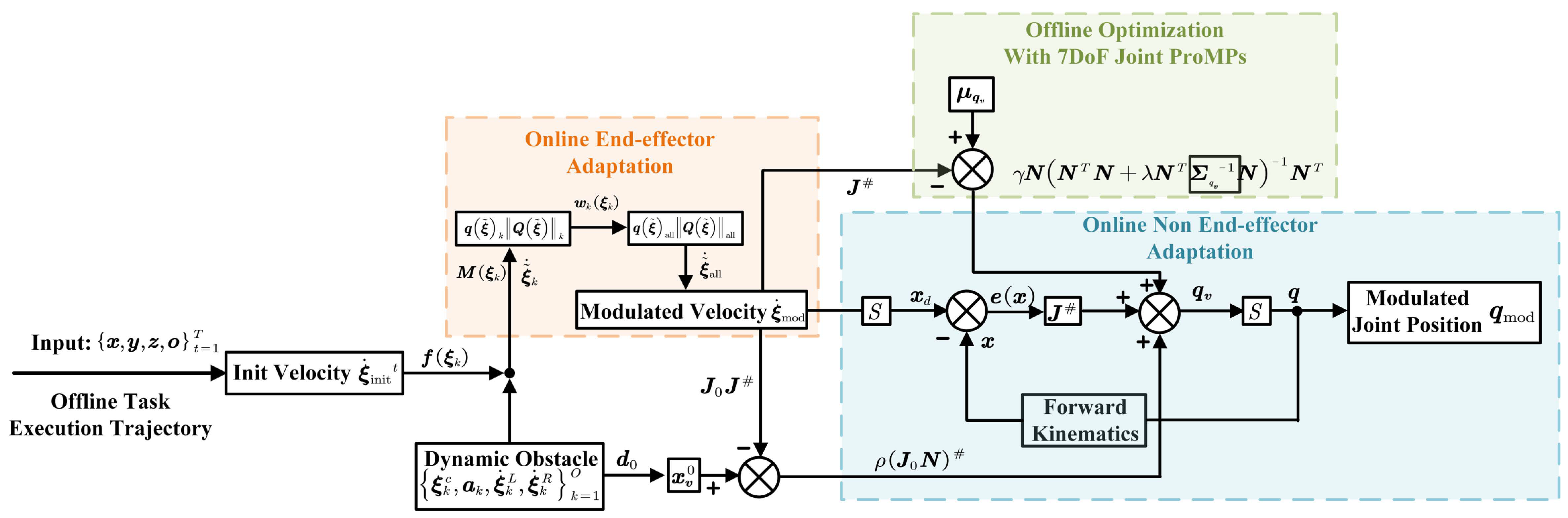
Considering real-time movement adaptation, during task execution, we propose an improved robot whole-body movement adaptation method, combining offline task-constrained optimization. For the robot end-effector, we incorporate an offline-optimized trajectory for dynamic modulation and develop DSM by performing multiple modulation iterations until safe; for the robot non-end-effector, we integrate the offline-optimized Joint ProMPs to improve the real-time null space velocity control method to ensure collision-free joint configurations through iterations.

4.

We conduct both offline and online movement adaptation experiments with comparative results to validate the effectiveness of the proposed strategy.

2. Via-Point Trajectory Generalization and Initial Distributions Encoding

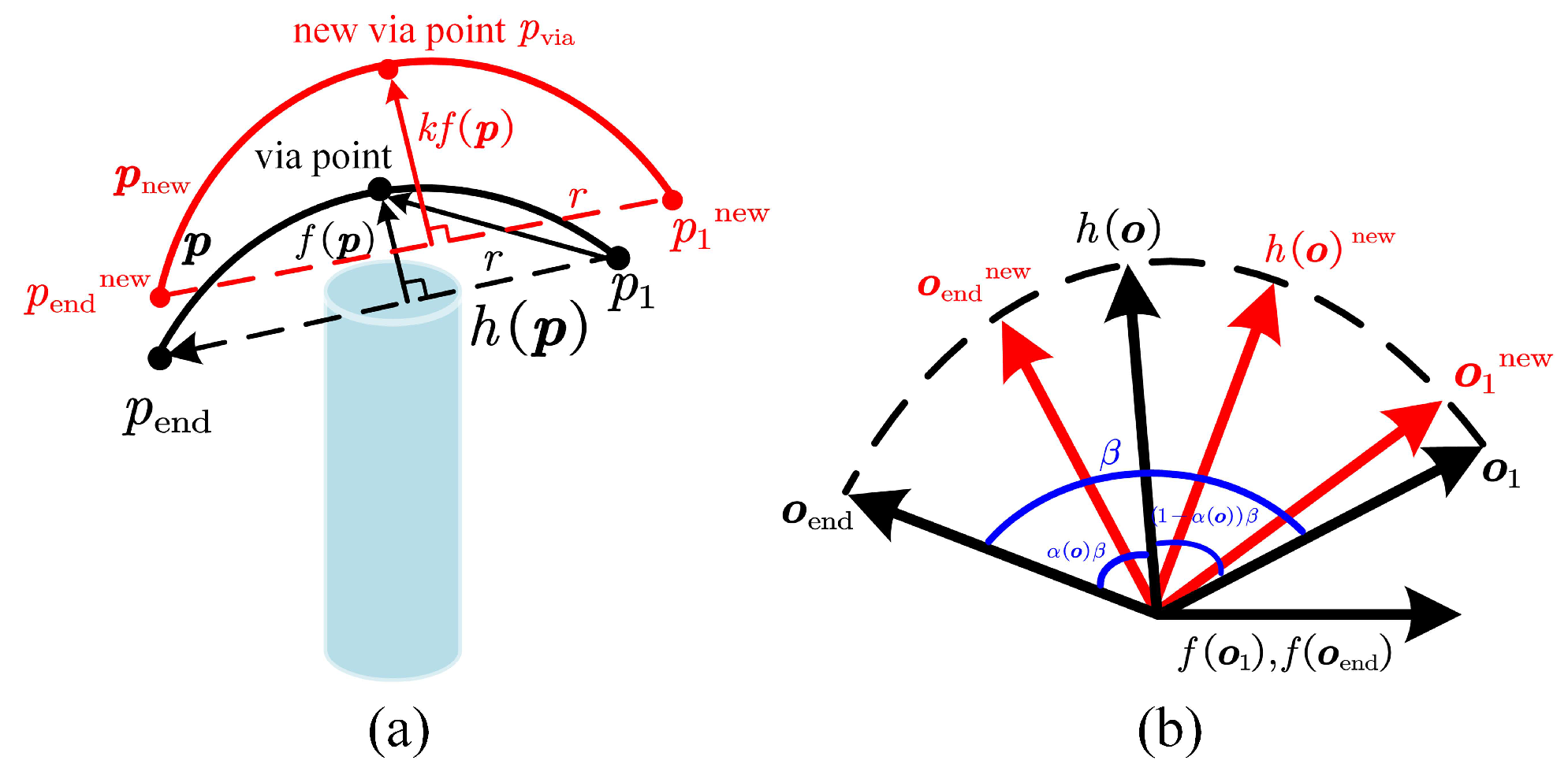
2.1. Learning New Skills in Cartesian Space with Via-Point Trajectory Generalization

To endow the robot with skill diversity for obstacle avoidance, the human provides three modes, namely, moving above, left, and right around the obstacle. For each mode, only one human demonstration is required, and we utilize a markerless vision capture system, the Kinect FORTH [37], to track human hand centroid movements with position and orientation sets $\left\{x,y,z,o_x,o_y,o_z,o_w\right\}$ recorded in T timesteps. We adopt the Moving Average Filter (MAF) to ensure smoothness and transform to the robot base frame via hand-eye calibration.

To learn skills denoted as positions and quaternions in Cartesian space, we express the demonstration trajectory as an integration of linear elementary trajectory h and nonlinear shape modulation f, and the schematic diagram of the proposed via-point trajectory generalization is shown in Figure 1.

For 3D positions, where each degree of freedom (DOF) is independent, we derive position sets $\mathit{p}$ with T timesteps in one DOF as follows:

$$y\left(\mathit{p}\right)=h\left(\mathit{p}\right)+f\left(\mathit{p}\right)$$

(1)

The elementary trajectory $h\left(\mathit{p}\right)$ is a line directly connecting the start point $p_1$ and the end point $p_{\mathrm{end}}$, with the shape modulation $f\left(\mathit{p}\right)$ defined as follows:

$$f\left(\mathit{p}\right)=\mathit{p}-\left(p_1+r\overrightarrow{p_1{p}_{\mathrm{end}}}\right)$$

(2)

where r is the scale factor denoting the proportion of projective points on the line $h\left(\mathit{p}\right)$,

$$r={\displaystyle \frac{\overrightarrow{p_1\mathit{p}}.\overrightarrow{p_1{p}_{\mathrm{end}}}}{\overrightarrow{p_1{p}_{\mathrm{end}}}.\overrightarrow{p_1{p}_{\mathrm{end}}}}}$$

(3)

If no intermediate via-points are required to generalize, we directly generate new projective points between the new start point $p_1^{\mathrm{new}}$ and end point $p_{\mathrm{end}}^{\mathrm{new}}$ according to r, and add learned shape modulation $f\left(\mathit{p}\right)$ to generalize new trajectory sets ${\mathit{p}}^{\mathrm{new}}$:

$${\mathit{p}}^{\mathrm{new}}=p_1^{\mathrm{new}}+r\overrightarrow{p_1^{\mathrm{new}}{p}_{\mathrm{end}}^{\mathrm{new}}}+f\left(\mathit{p}\right)$$

(4)

Once a via-point $\left(t_{\mathrm{via}},p_{\mathrm{via}}\right)$ is needed, we scale the shape modulation with the coefficient k:

$$k=\left|p_{\mathrm{via}}-\left(p_1^{\mathrm{new}}+r\overrightarrow{p_1^{\mathrm{new}}{p}_{\mathrm{end}}^{\mathrm{new}}}\right)\right|{\left|f\left(\mathit{p}\right)\right|}^{-1}$$

(5)

Subsequently, new trajectory sets ${\mathit{p}}^{\mathrm{new}}$ are generalized upon:

$${\mathit{p}}^{\mathrm{new}}=p_1^{\mathrm{new}}+r\overrightarrow{p_1^{\mathrm{new}}{p}_{\mathrm{end}}^{\mathrm{new}}}+kf\left(\mathit{p}\right)$$

(6)

For quaternion sets, considering dimensions are affected by each other in orientation, we define the trajectory with:

$$y\left(\mathit{o}\right)=h\left(\mathit{o}\right)\times f\left(\mathit{o}\right)$$

(7)

where $\mathit{o}=\left[{\mathit{o}}_{\mathrm{w}},{\mathit{o}}_{\mathrm{x}},{\mathit{o}}_{\mathrm{y}},{\mathit{o}}_{\mathrm{z}}\right]$ represents the quaternion sets, and × denotes quaternion multiplication. The elementary trajectory $h\left(\mathit{o}\right)$ is derived using the spherical linear interpolation (SLERP) as follows:

$$h\left(\mathit{o}\right)={\displaystyle \frac{sin\left(\left(1-\alpha \left(\mathit{o}\right)\right)\beta \right)}{sin\left(\beta \right)}}h\left({\mathit{o}}_1\right)+{\displaystyle \frac{sin\left(\alpha \left(\mathit{o}\right)\beta \right)}{sin\left(\beta \right)}}h\left({\mathit{o}}_{\mathrm{end}}\right)$$

(8)

where $cos\left(\beta \right)=h\left({\mathit{o}}_1\right).h\left({\mathit{o}}_{\mathrm{end}}\right)$, $\alpha \left(\mathit{o}\right)$ is the ratio of SLERP, ranging from 0 to 1. $h\left({\mathit{o}}_1\right)$ and $h\left({\mathit{o}}_{\mathrm{end}}\right)$ are the start and end points of the elementary trajectory:

$$h\left({\mathit{o}}_1\right)=y\left({\mathit{o}}_1\right)\times f{\left({\mathit{o}}_1\right)}^{-1},h\left({\mathit{o}}_{\mathrm{end}}\right)=y\left({\mathit{o}}_{\mathrm{end}}\right)\times f{\left({\mathit{o}}_{\mathrm{end}}\right)}^{-1}$$

(9)

In order to learn $f\left(\mathit{o}\right)$ from demonstration, we set $\alpha \left(\mathit{o}\right)$ to distribute uniformly over T timesteps and set $f\left({\mathrm{o}}_1\right)$, $f\left({\mathit{o}}_{\mathrm{end}}\right)$ to $\left[1,0,0,0\right]$. Once new start quaternion sets ${\mathit{o}}_1^{\mathrm{new}}$ and end quaternion sets ${\mathit{o}}_{\mathrm{end}}^{\mathrm{new}}$ are required during generalization, we compute a new elementary trajectory $h{\left(\mathit{o}\right)}^{\mathrm{new}}$ using Equations (8) and (9), with learned shape modulation $f\left(\mathit{o}\right)$ superimposed to generate a new orientation trajectory $y{\left(\mathit{o}\right)}^{\mathrm{new}}$ using Equation (7). Note that there is no need to generalize via-points in orientation, as we can achieve via-points generalization in 3D positions while keeping the original orientations.

2.2. Model Joint Space Distributions with Probabilistic Movement Primitives

Probabilistic Movement Primitives (ProMPs) [10] are probabilistic methods based on hierarchical Bayesian models to encode variances in Joint or Cartesian space. To promote integrating all nonlinear task constraints for the robot end effector and other links analytically, we model the Joint space distributions with ProMPs. Given the positions and orientations ${\left\{{\mathit{x}}_t,{\mathit{y}}_t,{\mathit{z}}_t,{\mathit{o}}_t\right\}}_{i=1}^N$ generalized in Section 2.1, we obtain all feasible joint sets ${\left\{{\mathit{q}}_t\right\}}_{i=1}^N=F_{\mathrm{IK}}\left({\left\{{\mathit{x}}_t,{\mathit{y}}_t,{\mathit{z}}_t,{\mathit{o}}_t\right\}}_{i=1}^N\right)$ by the Jacobian inverse kinematic (IK) algorithm [38]. ${\mathit{q}}_t\in {\mathbb{R}}^D$, $t\in \left[0,T\right]$, N is the number of demonstrations, and D is the joint DOFs.

ProMPs model joint positions as a linear combination of Gaussian basis functions $\mathbf{\Psi }\left(t\right)$ and a weight vector ${\mathit{w}}_i$ under the presence of a zero-mean Gaussian noise ${\mathit{\epsilon }}_n$,

$${\mathit{q}}_i\left(t\right)=\mathbf{\Psi }{\left(t\right)}^T{\mathit{w}}_i+{\epsilon }_n$$

(10)

Joint positions in one demonstration are expressed with the weight vector ${\mathit{w}}_i$ via linear ridge regression [39]. Using parameters $\mathit{\theta }=\left\{{\mathit{\mu }}_{\mathit{w}},{\mathbf{\Sigma }}_{\mathit{w}}\right\}$ to estimate the weight vector $\mathit{w}$ with Gaussian distributions $p\left(\mathit{w};\mathit{\theta }\right)=\mathcal{N}\left(\mathit{w}|{\mathit{\mu }}_{\mathit{w}},{\mathbf{\Sigma }}_{\mathit{w}}\right)$, the probability of observing a trajectory $\mathit{\tau }$ given $\mathit{\theta }$ becomes:

$$\begin{array}{cc}\hfill & p\left(\mathit{\tau };\mathit{\theta }\right)=p\left(\mathit{\tau }|\mathit{w}\right)p\left(\mathit{w};\mathit{\theta }\right)d\mathit{w}\hfill \\ \hfill & =\prod _t\mathcal{N}\left(\left.\mathit{q}\left(t\right)\right|\mathbf{\Psi }{\left(t\right)}^T{\mathit{\mu }}_{\mathit{w}},\mathbf{\Psi }{\left(t\right)}^T{\mathbf{\Sigma }}_{\mathit{w}}\mathbf{\Psi }\left(t\right)+{\mathbf{\Sigma }}_n\right)\hfill \end{array}$$

(11)

where ${\mathit{\mu }}_{\mathit{w}}$ and ${\mathbf{\Sigma }}_{\mathit{w}}$ denote the mean and covariance of the weight vector, which are derived by maximum likelihood estimation, and ${\mathbf{\Sigma }}_n$ is the covariance of the Gaussian noise. When it comes to new task conditions ${\mathit{Q}}^{*}=\left[{\mathit{q}}^{*},{\mathbf{\Sigma }}_q^{*}\right]$, where ${\mathit{q}}^{*}$ and ${\mathbf{\Sigma }}_q^{*}$ are the expected mean and covariance of the joint positions at time t, the updated parameters ${\mathit{\theta }}^{\mathrm{new}}=\left\{{\mathit{\mu }}_{\mathit{w}}^{\mathrm{new}},{\mathbf{\Sigma }}_{\mathit{w}}^{\mathrm{new}}\right\}$ can be computed based on Bayesian theory as follows:

$$p\left(\left.\mathit{w}\right|{\mathit{Q}}^{*}\right)\propto \mathcal{N}\left(\left.{\mathit{Q}}^{*}\right|{\mathbf{\Psi }*}^T\mathit{w},{\mathbf{\Sigma }}_q^{*}\right)p\left(\mathit{w}\right)$$

(12)

$$\begin{array}{cc}\hfill & {\mathit{\mu }}_{\mathit{w}}^{\mathrm{new}}={\mathit{\mu }}_{\mathit{w}}+{\mathbf{\Sigma }}_{\mathit{w}}{\mathbf{\Psi }}^{*}{\left({\mathbf{\Sigma }}_q^{*}+{\mathbf{\Psi }*}^T{\mathbf{\Sigma }}_{\mathit{w}}{\mathbf{\Psi }}^{*}\right)}^{-1}\left({\mathit{q}}^{*}-{\mathbf{\Psi }*}^T{\mathit{\mu }}_{\mathit{w}}\right)\hfill \\ \hfill & {\mathbf{\Sigma }}_{\mathit{w}}^{\mathrm{new}}={\mathbf{\Sigma }}_{\mathit{w}}-{\mathbf{\Sigma }}_{\mathit{w}}{\mathbf{\Psi }}^{*}{\left({\mathbf{\Sigma }}_q^{*}+{\mathbf{\Psi }*}^T{\mathbf{\Sigma }}_{\mathit{w}}{\mathbf{\Psi }}^{*}\right)}^{-1}{\mathbf{\Psi }*}^T{\mathbf{\Sigma }}_{\mathit{w}}\hfill \end{array}$$

(13)

where ${\mathbf{\Psi }}^{*}$ denotes the basis function at time t. The Joint positions under new task conditions ${\mathit{p}}^{\mathrm{new}}$ are sampled from Gaussian distributions as follows:

$$\begin{array}{cc}\hfill & {\mathit{w}}^{\mathrm{new}}\sim \mathcal{N}\left({\mathit{\mu }}_{\mathit{w}}^{\mathrm{new}},{\mathbf{\Sigma }}_{\mathit{w}}^{\mathrm{new}}\right)\hfill \\ \hfill & {\mathit{p}}^{\mathrm{new}}={\mathbf{\Psi }}^T{\mathit{w}}^{\mathrm{new}}\hfill \end{array}$$

(14)

3. Offline Optimization and Adaptation Under Nonlinear Task Constraints

After generalizing feasible collision-free trajectories with initial ProMPs distribution encoded, we put forward the optimization method under various nonlinear task constraints. Given optimized ProMPs distribution, we present the movement adaptation method for task execution. We formulate the constrained optimization problem in Section 3.1, provide analytical expressions of task constraints in Section 3.2, and summarize the complete procedure in Section 3.3.

3.1. Problem Formulation

Given initial ProMPs distribution $p_0\left(\mathit{w}\right)=\mathcal{N}\left(\mathit{w};{\mathit{\mu }}_{\mathit{w}}^0,{\mathbf{\Sigma }}_{\mathit{w}}^0\right)$, the main objective is to obtain the optimized ProMPs distribution $p\left({\mathit{w}}^{*}\right)=\mathcal{N}\left({\mathit{w}}^{*};{\mathit{\mu }}_{\mathit{w}}^{*},{\mathbf{\Sigma }}_{\mathit{w}}^{*}\right)$, which is as close as possible to the original distribution while satisfying task constraints. We use the Kullback–Leibler divergence to represent the similarity between optimized and initial distributions owing to its analytical tractability, while expressing the constraints with cumulative distribution functions. However, in this paper, considering ProMPs model every timestep as an independent Gaussian distribution, we optimize the parameters of each timestep separately. Specifically, we convert the initial distribution $p_0\left(\mathit{w}\right)=\mathcal{N}\left(\mathit{w};{\mathit{\mu }}_{\mathit{w}}^0,{\mathbf{\Sigma }}_{\mathit{w}}^0\right)$ to the mean and standard deviation $\left({\mathit{\mu }}_t^0,{\mathit{\sigma }}_t^0\right)$ of each timestep t as follows:

$$\begin{array}{cc}\hfill & {\mathit{\mu }}_t^0={\mathbf{\Psi }}_t^T{\mathit{\mu }}_{\mathit{w}}^0\hfill \\ \hfill & {\mathit{\sigma }}_t^0=\mathrm{sqrt}\left({\mathbf{\Psi }}_t^T{\mathbf{\Sigma }}_{\mathit{w}}^0{\mathbf{\Psi }}_t\right)\hfill \end{array}$$

(15)

For each timestep t, the new mean and standard deviation $\left({\mathit{\mu }}_t^{*},{\mathit{\sigma }}_t^{*}\right)$ are optimized under task constraints separately. Let $c_{k,t}=C\left({\mathit{\mu }}_t,{\mathit{\sigma }}_t\right)$ denote the function of the $k^{th}$ task constraints related to $\left({\mathit{\mu }}_t,{\mathit{\sigma }}_t\right)$, and $F_{{\mathrm{c}}_{k,t}}\left({\mathit{\mu }}_t,{\mathit{\sigma }}_t\right)$ denote the cumulative distribution function (CDF) of the random variable defined by $c_{k,t}$, then we can rewrite the optimization problem as a Lagrangian function:

$$\begin{array}{cc}\hfill L\left({\mathit{\mu }}_t,{\mathit{\sigma }}_t,\left\{{\lambda }_{k,t}\right\}\right)=& {\mathrm{D}}_{\mathrm{KL}}\left[\mathcal{N}\left({\mathit{q}}_t;{\mathit{\mu }}_t,{\mathit{\sigma }}_t\right)\left|\right|\mathcal{N}\left({\mathit{q}}_t^0;{\mathit{\mu }}_t^0,{\mathit{\sigma }}_t^0\right)\right]\hfill \\ \hfill & +\sum _{k,t}{\lambda }_{k,t}\left[{\alpha }_{k,t}-F_{c_{k,t}}\left({\mathit{\mu }}_t,{\mathit{\sigma }}_t\right)\right]\hfill \end{array}$$

(16)

where ${\alpha }_{k,t}$ is the confidence level to represent the probability satisfying task constraints $P_{{\mathit{\mu }}_t,{\mathit{\sigma }}_t}\left(H\left(c_{k,t}\right)\right)⩾{\alpha }_{k,t}$, and H represents the one-side or two-side inequality constraints; the optimized mean and standard deviation $\left({\mathit{\mu }}_t^{*},{\mathit{\sigma }}_t^{*}\right)$ are derived by gradient ascent-descent methods as follows:

$$\left({\mathit{\mu }}_t^{*},{\mathit{\sigma }}_t^{*},\left\{{\lambda }_{k,t}^{*}\right\}\right)=\underset{{\lambda }_{k,t}⩾0}{max}\underset{{\mathit{\mu }}_t,{\mathit{\sigma }}_t}{min}L\left({\mathit{\mu }}_t,{\mathit{\sigma }}_t,\left\{{\lambda }_{k,t}\right\}\right)$$

(17)

Subsequently, given $\left({\mathit{\mu }}_t^{*},{\mathit{\sigma }}_t^{*}\right)$, we implement another optimization step to obtain the optimized ProMPs distribution $\left({\mathit{\mu }}_{\mathit{w}}^{*},{\mathbf{\Sigma }}_{\mathit{w}}^{*}\right)$ with:

$$\begin{array}{cc}\hfill {\mathit{\mu }}_{\mathit{w}}^{*}& =\underset{{\mathit{\mu }}_{\mathit{w}}}{min}\left({\mathbf{\Psi }}_t^T{\mathit{\mu }}_{\mathit{w}}-{\mathit{\mu }}_t^{*}\right)\hfill \\ \hfill {\mathbf{\Sigma }}_{\mathit{w}}^{*}& =\underset{{\mathbf{\Sigma }}_{\mathit{w}}}{min}\left({\mathbf{\Psi }}_t^T{\mathbf{\Sigma }}_{\mathit{w}}{\mathbf{\Psi }}_t-{\mathit{\sigma }}_t^{*}\right)\hfill \end{array}$$

(18)

In Section 3.2, we formulate every task constraint by defining the function $c_{k,t}=C\left({\mathit{\mu }}_t,{\mathit{\sigma }}_t\right)$ related to $\left({\mathit{\mu }}_t,{\mathit{\sigma }}_t\right)$, expressing the inequality constraint function H and approximating the cumulative distribution function $F_{{\mathrm{c}}_{k,t}}\left({\mathit{\mu }}_t,{\mathit{\sigma }}_t\right)$; the optimized results are then numerically iterated based on automatic differentiation.

3.2. Constraints Definitions in Joint Space and Cartesian Space

A robot may encounter constraints in Joint space and Cartesian space at one time. Joint space constraints depend directly on $\left({\mathit{\mu }}_t,{\mathit{\sigma }}_t\right)$ of each joint freedom, which usually refer to the motion range of the robot’s links. The Cartesian space constraints depend on the nonlinear forward kinematics function of $\left({\mathit{\mu }}_t,{\mathit{\sigma }}_t\right)$, standing for the 3D positions of the end effector or any other interest points on the robot links. In the following, we formulate several key constraints commonly used in obstacle avoidance, like the joint range limit, waypoints, hyperplane, and repellers.

3.2.1. Joint Range Limit

The joint range limit indicates the limit motion range in joint space based on the robot’s configuration or the user’s expectation. Considering the limit motion range is usually ensured with the forward kinematics (FK) function. In this paper, we focus on retaining the original joint range limit learned with ProMPs as much as possible. We formulate the constraint function as $c_{k,t}={\mathit{q}}_t\left({\mathit{\mu }}_t,{\mathit{\sigma }}_t\right)$, and denote the two-side constraint with:

$$P_{{\mathit{\mu }}_t,{\mathit{\sigma }}_t}\left({\mathit{q}}_{k,t}^{min}<{\mathit{q}}_t\left({\mathit{\mu }}_t,{\mathit{\sigma }}_t\right)<{\mathit{q}}_{k,t}^{max}\right)⩾{\alpha }_{k,t}$$

(19)

where k denotes the kth joint freedom, ${\alpha }_{k,t}$ is the confidence level, and ${\mathit{q}}_{k,t}^{min}$ and ${\mathit{q}}_{k,t}^{max}$ are the minimum and maximum of the joint positions from demonstration, respectively. Due to the Gaussian distributions of the joint positions, we calculate the difference between the CDF of the maximum and minimum points as follows:

$$F_{c_{k,t}}\left({\mathit{\mu }}_t,{\mathit{\sigma }}_t\right)=F\left({\displaystyle \frac{{\mathit{q}}_{k,t}^{max}-{\mathit{\mu }}_t}{{\mathit{\sigma }}_t}}\right)-F\left({\displaystyle \frac{{\mathit{q}}_{k,t}^{min}-{\mathit{\mu }}_t}{{\mathit{\sigma }}_t}}\right)$$

(20)

where F denotes the CDF of the Gaussian distributions.

3.2.2. Waypoints

Waypoints are Cartesian positions ${\overline{\mathit{X}}}_t$ on the robot’s end effector or any other interest points that we expect the robot to reach at timestep t or a temporal interval $\mathcal{T}\subset \left[0,T\right]$. Waypoints are defined in the Cartesian space with the FK function T to associate with some DOFs of the joint positions. Based on the distance square between the expected points and the actual points, we denote the waypoint constraint function as follows:

$$c_{k,t}={|T\left({\mathit{q}}_t\left({\mathit{\mu }}_t,{\mathit{\sigma }}_t\right)\right)-{\overline{\mathit{X}}}_t|}^2$$

(21)

And express the one-side constraint with:

$$P_{{\mathit{\mu }}_t,{\mathit{\sigma }}_t}\left(|T\left({\mathit{q}}_t\left({\mathit{\mu }}_t,{\mathit{\sigma }}_t\right)\right)-{\overline{\mathit{X}}}_t{|}^2⩽d_{k,t}^2\right)⩾{\alpha }_{k,t}$$

(22)

where $d_{k,t}$ is the distance threshold and ${\alpha }_{k,t}$ is the confidence level. Due to the nonlinear nature of the constraint function, we can not derive the exact distribution of $c_{k,t}$ with Bayesian theory. To tackle the problem, the Unscented Transform [40] method is adopted in [21]. However, the initial factor deeply influences the estimation result—when the mean and standard deviation change, the factor can not reflect the variance of the constraint function precisely. Alternatively, in this paper, we utilize moment matching to estimate the $c_{k,t}$ distribution:

$$\begin{array}{cc}\hfill S=\{c_{k,t}\left({\mathit{q}}_1,{\mathit{q}}_2,\dots ,{\mathit{q}}_D\right),{\mathit{q}}_k& \in \{{\mathit{\mu }}_k-2{\mathit{\sigma }}_k,{\mathit{\mu }}_k+2{\mathit{\sigma }}_k\}\}\hfill \\ \hfill \mathrm{E}\left(c_{k,t}\right)\approx & \mathrm{Mean}\left[S\right]\hfill \\ \hfill \mathrm{V}\left(c_{k,t}\right)\approx & \mathrm{Var}\left[S\right]\hfill \end{array}$$

(23)

where D is the DOF number required to express the constraint function. We utilize 2x the standard deviation to constitute the set S and compute the mean and variance based on moment-matching. Given that the distribution of the random variable $c_{k,t}$ is a generalized-${\chi }^2$, we approximate it with a simpler Gamma distibution to represent the CDF in an analytical way. The shape $\alpha$ and rate $\beta$ of the Gamma distribution are derived as follows:

$$\begin{array}{cc}\hfill c_{k,t}& \sim \mathsf{\Gamma }\left(\alpha ,\beta \right)\hfill \\ \hfill \alpha =\mathrm{E}{\left(c_{k,t}\right)}^2/\mathrm{V}\left(c_{k,t}\right),& \beta =\mathrm{E}\left(c_{k,t}\right)/\mathrm{V}\left(c_{k,t}\right)\hfill \end{array}$$

(24)

The CDF of the Gamma distributions are then computed using $F_{c_{k,t}}=F\left(d_{k,t};\mathsf{\Gamma }\left(\alpha ,\beta \right)\right)$ to represent the waypoints constraint probability via Equation (22).

3.2.3. Hyperplane

During motion, the robot is required to be confined to specific planes called the hyperplane or the virtual wall. Hyperplane constraints are defined in the Cartesian space related to the positions of the robot’s end effector or any other interest points. We can formulate a hyperplane constraint function as follows:

$$c_{k,t}={\mathit{n}}_{k,t}^T\left(T\left({\mathit{q}}_t\left({\mathit{\mu }}_t,{\mathit{\sigma }}_t\right)\right)-{\mathit{b}}_{k,t}\right)$$

(25)

where ${\mathit{n}}_{k,t}$ and ${\mathit{b}}_{k,t}$ are the normal and bias vectors of the hyperplane. The one-side inequality constraint is expressed with:

$$P_{{\mathit{\mu }}_t,{\mathit{\sigma }}_t}\left({\mathit{n}}_{k,t}^T\left(T\left({\mathit{q}}_t\left({\mathit{\mu }}_t,{\mathit{\sigma }}_t\right)\right)-{\mathit{b}}_{k,t}\right)⩽0\right)⩾{\alpha }_{k,t}$$

(26)

The distribution of $c_{k,t}$ is a linear transformation of the robot’s 3D positions $T\left({\mathit{q}}_t\left({\mathit{\mu }}_t,{\mathit{\sigma }}_t\right)\right)$; however, $T\left({\mathit{q}}_t\left({\mathit{\mu }}_t,{\mathit{\sigma }}_t\right)\right)$ is nonlinear in $\left({\mathit{\mu }}_t,{\mathit{\sigma }}_t\right)$. We thus use our moment-matching method via Equation (23) to obtain the estimated mean $\mathrm{E}\left[T\right]$ and variance $\mathrm{V}\left[T\right]$. The overall distribution of $c_{k,t}$ can be derived by:

$$c_{k,t}\sim \mathcal{N}\left(\begin{array}{c}{\mathit{n}}_{k,t}^T\left(\mathrm{E}\left[T\right]\right)-{\mathit{b}}_{k,t},{\mathit{n}}_{k,t}^T\mathrm{V}\left[T\right]{\mathit{n}}_{k,t}\end{array}\right)$$

(27)

Subsequently, The CDF of $c_{k,t}$ is computed using Gaussian distributions to represent the hyperplane constraint probability via Equation (26). Note that we can impose hyperplane constraints at a timestep or a temporal interval, and combine several hyperplane constraints to represent more complex convex domains.

3.2.4. Repellers

The robot needs to avoid obstacles in the environment while performing tasks. Constraints between the robot and obstacles are called repeller constraints. Repellers constraints are imposed not only on the robot end effector but also on any other danger points on the robot link. In this paper, we choose three segments on the robot link in each direction: front, back, left and right, and use cylinders to envelop obstacles. Considering we only need to consider danger situations where the robot is apt to collide, we define the danger distance to express the repellers constraints. For three segments in four directions, we compute the shortest distance between segments on the robot link and the axis segment, with the minimum distance $d_{min}$ found afterward. If the minimum distance is greater than the safety radius $R_{\mathrm{safe}}$ of obstacles, the danger distance $d_{\mathrm{danger}}$ is 0, and if else, the danger distance is computed as $d_{\mathrm{danger}}=R_{\mathrm{safe}}-d_{min}$. We formulate the repellers constraint function as follows:

$$c_{k,t}=\left\{\begin{array}{c}0,d_{min}⩾R_{\mathrm{safe}}\hfill \\ R_{\mathrm{safe}}-d_{min}\left(T\left({\mathit{q}}_t\left({\mathit{\mu }}_t,{\mathit{\sigma }}_t\right)\right)\right),d_{min}<R_{\mathrm{safe}}\hfill \end{array}\right.$$

(28)

Furthermore, we express the one-side inequality constraint to show the probability that the minimum distance is greater than the safety radius:

$$P_{{\mathit{\mu }}_t,{\mathit{\sigma }}_t}\left(c_{k,t}⩽0\right)⩾{\alpha }_{k,t}$$

(29)

The distribution of $c_{k,t}$ is nonlinear in $\left({\mathit{\mu }}_t,{\mathit{\sigma }}_t\right)$. We thus utilize our moment-matching method with Equation (23) to obtain the mean and variance of $c_{k,t}$. The CDF of $c_{k,t}$ is then computed using Gaussian distributions to denote the repellers constraint probability with Equation (29).

3.3. Optimization and Adaptation Procedure

3.3.1. Optimization Procedure

Based on the Lagrangian function in Equation (16) and constraints function defined in Section 3.2, we concretize the optimization procedure to obtain the optimal parameters. For notational brevity, we use the notation ${\mathit{\theta }}_0=\left({\mathit{\mu }}_t^0,{\mathit{\sigma }}_t^0\right)$ and $\mathit{\theta }=\left({\mathit{\mu }}_t,{\mathit{\sigma }}_t\right)$ to denote the intial parameters and optimized parameters. We can rewrite the Lagrangian function in Equation (16) as follows:

$$L\left(\mathit{\theta },\left\{{\lambda }_{k,t}\right\}\right)={\mathrm{D}}_{\mathrm{KL}}\left[\mathit{\theta }\left|\right|{\mathit{\theta }}_0\right]+\sum _{k,t}{\lambda }_{k,t}\left({\alpha }_{k,t}-F_{c_{k,t}}\left(\mathit{\theta }\right)\right)$$

(30)

The term ${\mathrm{D}}_{\mathrm{KL}}\left[\mathit{\theta }\left|\right|{\mathit{\theta }}_0\right]$ denoting the KL divergence between two univariate Gaussian distributions is further derived by:

$${\mathrm{D}}_{\mathrm{KL}}\left[\mathit{\theta }\left|\right|{\mathit{\theta }}_0\right]=-{\displaystyle \frac{1}{2}}+log\left({\mathit{\sigma }}^0\right)-log\left(\mathit{\sigma }\right)+{\displaystyle \frac{{\mathit{\sigma }}^2+{\left(\mathit{\mu }-{\mathit{\mu }}^0\right)}^2}{2{\left({\mathit{\sigma }}^0\right)}^2}}$$

(31)

We express the optimized parameters derived in Equation (17) as follows:

$$\left({\mathit{\theta }}^{*},\left\{{\lambda }_{k,t}^{*}\right\}\right)=\underset{{\lambda }_{k,t}⩾0}{max}\underset{\mathit{\theta }}{min}L\left(\mathit{\theta },\left\{{\lambda }_{k,t}\right\}\right)$$

(32)

To solve the problem, we utilize a double-loop algorithm based on the gradient ascent-descent method. For the outer-loop, we optimize ${\lambda }_{k,t}$ with the gradient quasi-ascent steps. The Exponential Method of Multipliers (EMM) [41] method is suitable to solve the inequality constraints of the Lagrangian function via exponential factors. We can express the optimized ${\lambda }_{k,t}$ after each iteration as ${\lambda }_{k,t}^{\left(s+1\right)}={\lambda }_{k,t}^{\left(s\right)}.exp\left\{{\eta }_k{\partial }_{{\lambda }_{k,t}}L\right\}$, where ${\eta }_k$ decides the convergence speed; the gradient of $\left\{{\lambda }_{k,t}\right\}$ is obtained by ${\partial }_{{\lambda }_{k,t}}L={\alpha }_{k,t}-F_{c_{k,t}}\left(\mathit{\theta }\right)$. For the inner-loop, we optimize $\mathit{\theta }$ with the gradient descent method. The LBFGS method [42] is tailored for solving nonlinear optimization problems with low computing and memory costs. We perform several LBFGS steps in $\mathit{\theta }$, with the gradient ${\partial }_{\mathit{\theta }}L$ computed using the automatic differentiation frameworks in Tensorflow [43]. The convergence conditions are checked after each iteration of LBFGS to speed up convergence. After we obtain the optimized $\left({\mathit{\mu }}_t^{*},{\mathit{\sigma }}_t^{*}\right)$, we directly perform several LBFGS steps to obtain the optimized $\left({\mathit{\mu }}_{\mathit{w}}^{*},{\mathbf{\Sigma }}_{\mathit{w}}^{*}\right)$ based on Equation (18).

3.3.2. Adaptation Procedure

Subsequently, given optimized ProMPs distribution $\left({\mathit{\mu }}_{\mathit{w}}^{*},{\mathbf{\Sigma }}_{\mathit{w}}^{*}\right)$, we present the complete offline robot movement adaptation procedure. During the learning phase, the human first demonstrates three skills to avoid a single obstacle. The human hand centroid positions and orientations are equivalent to the robot end effector trajectories. For each mode, we generalize trajectory sets to the same start and end points, normalized to the same timestep T, to formulate the template trajectory. Aiming to generate feasible collision-free trajectory sets, we choose feature 3D via-points with equal intervals to generalize the initial trajectories (see Section 2.1). We check the collisions and fine-tune the via-points with threshold to construct initial collision-free trajectories ${\left\{\mathit{x},\mathit{y},\mathit{z},{\mathit{o}}_{\mathrm{x}},{\mathit{o}}_{\mathrm{y}},{\mathit{o}}_{\mathrm{z}},{\mathit{o}}_{\mathrm{w}}\right\}}_{i=1}^N$ and obtain corresponding joint position sets ${\left\{\mathit{q}\right\}}_{i=1}^N$. We encode the initial joint distributions with ProMPs (see Section 2.2) as $p_0\left(\mathit{w}\right)=\mathcal{N}\left(\mathit{w};{\mathit{\mu }}_{\mathit{w}}^0,{\mathbf{\Sigma }}_{\mathit{w}}^0\right)$. To speed up optimization, we first find feature timesteps that actually violate task constraints, then impose task constraints at those timesteps ${\mathit{t}}_{\mathrm{feature}}$ and optimize the ProMPs distributions (see Section 3.3.1). The optimized ProMPs $p\left({\mathit{w}}^{*}\right)=\mathcal{N}\left({\mathit{w}}^{*};{\mathit{\mu }}_{\mathit{w}}^{*},{\mathbf{\Sigma }}_{\mathit{w}}^{*}\right)$, the mean and standard deviation $p\left({\mathit{q}}_t\right)=\mathcal{N}\left({\mathit{q}}_t;{\mathit{\mu }}_t^{*},{\mathit{\sigma }}_t^{*}\right)$ are treated as safe joint distributions.

During task execution, the robot first determines the start and end point by visual information, next randomly selects the running mode from three modes $k\sim \left\{above,left,right\right\}$, then samples the via-points with Gaussian distributions as ${\mathit{p}}_{via}=\mathcal{N}\left({\mathit{\mu }}_{xyz},{\mathit{\sigma }}_{xyz}\right)$. The mean ${\mathit{\mu }}_{xyz}$ and standard deviation ${\mathit{\sigma }}_{xyz}$ are computed from the initial via-points range. The trajectory is then generalized and fine-tuned to ensure safety according to the sampled via-point. The optimized ${\mathit{\mu }}_t^{*}$ and ${\mathit{\sigma }}_t^{*}$ represent the joint limit range as ${\mathit{q}}_t^{\mathrm{safe}}\in \left({\mathit{\mu }}_t^{*}-2{\mathit{\sigma }}_t^{*},{\mathit{\mu }}_t^{*}+2{\mathit{\sigma }}_t^{*}\right)$ with the initial joint value denoted as ${\mathit{q}}_t^0={\mathbf{\Psi }}_t^T{\mathit{w}}^{*}$. The joint limited range and initial value are passed to the Jacobian IK algorithm to test whether the solution is calculated successfully. The succeed number of all feature timesteps decides whether the robot can perform the task successfully; that is, if the succeed number is more than a threshold, the robot directly runs the generalized trajectory, if else, the robot continues sampling until success. To obtain the threshold automatically, we perform equal space sampling from the initial via-points range, record the success result and corresponding succeed number, then determine the threshold at the turning point between success and failure. Note that if there are no feature timesteps that violate the task constraints, the robot only needs to generalize the trajectory without optimizing the distribution. Meanwhile, if any of the three modes can not be optimized, that is, the probability satisfying the task constraints always equals 0, we eliminate the mode from the optional modes. The complete offline optimization and adaptation procedure is outlined in Algorithm 1.

Algorithm 1 Robotic offline task constrained optimization and adaptation algorithm.

Input:  • Obstacles information $\left\{{\mathrm{obs}}_{\mathit{x}},{\mathrm{obs}}_{\mathit{y}},{\mathrm{obs}}_{\mathit{z}},\mathit{R}\right\}$  • Mode template trajectory ${\left\{\mathit{x},\mathit{y},\mathit{z},{\mathit{o}}_{\mathrm{x}},{\mathit{o}}_{\mathrm{y}},{\mathit{o}}_{\mathrm{z}},{\mathit{o}}_{\mathrm{w}}\right\}}_{k=1}^3$  • Global start point and end point $\left\{{\mathit{p}}_1,{\mathit{p}}_{\mathrm{end}}\right\}$ Output: Task execution trajectory $\left\{\mathit{x},\mathit{y},\mathit{z},{\mathit{o}}_{\mathrm{x}},{\mathit{o}}_{\mathrm{y}},{\mathit{o}}_{\mathrm{z}},{\mathit{o}}_{\mathrm{w}}\right\}$  □ Generalize collision-free trajectories and encode initial ProMPs  • Choose and fine-tune via-points to generate N safe trajectories  • Obtain feasible joint sets ${\left\{\mathit{q}\right\}}_{i=1}^N$ and encode with ProMPs $\left({\mathit{\mu }}_{\mathit{w}}^0,{\mathbf{\Sigma }}_{\mathit{w}}^0\right)$  □ Optimize ProMPs under nonlinear task constraints  • Find feature timesteps $\left\{{\mathit{t}}_{\mathrm{feature}}\right\}$ that violate task constraints  • Compute $\left({\mathit{\mu }}_t^0,{\mathit{\sigma }}_t^0\right)$ using Equation (15)  • Derive $c_{k,t}$, H and $F_{c_{k,t}}\left({\mathit{\mu }}_t,{\mathit{\sigma }}_t\right)$ (see Section 3.2) to construct Equation (16)  • ${\mathit{\theta }}^0\leftarrow {\mathit{\theta }}_0,\left\{{\lambda }_{k,t}^0\right\}$ defined in Equation (30)  • Optimisation 1: Learnable parameters 1: $\left({\mathit{\mu }}_t^{*},{\mathit{\sigma }}_t^{*},{\lambda }_{k,t}^{*}\right)$ in Equation (32)  repeat   repeat    ${\mathit{\theta }}^{\left(s+1\right)}\leftarrow$ LBFGS $\left(L,{\partial }_{\mathit{\theta }}L,{\mathit{\theta }}^{\left(s\right)},\left\{{\lambda }_{k,t}^{\left(r\right)}\right\}\right)$   until inner-loop-condition   ${\lambda }_{k,t}^{\left(r+1\right)}\leftarrow {\lambda }_{k,t}^{\left(r\right)}.exp\left\{{\eta }_k\left({\alpha }_{k,t}-F_{c_{k,t}}\left(\mathit{\theta }\right)\right)\right\}$  until converged  • Optimisation 2: Learnable parameters 2: $\left({\mathit{\mu }}_{\mathit{w}}^{*},{\mathbf{\Sigma }}_{\mathit{w}}^{*}\right)$ in Equation (18)  repeat   $\left({\mathit{\mu }}_{\mathit{w}}^{\left(\mathrm{s}+1\right)},{\mathbf{\Sigma }}_{\mathit{w}}^{\left(\mathrm{s}+1\right)}\right)\leftarrow$ LBFGS $\left({\mathit{\mu }}_{\mathit{w}}^{\left(\mathrm{s}\right)},{\mathbf{\Sigma }}_{\mathit{w}}^{\left(\mathrm{s}\right)},{\mathit{\mu }}_t^{*},{\mathit{\sigma }}_t^{*}\right)$  until converged  • Obtain optimized joint limit range and initial joint value ${\mathit{q}}_t^{\mathrm{safe}}\in \left({\mathit{\mu }}_t^{*}-2{\mathit{\sigma }}_t^{*},{\mathit{\mu }}_t^{*}+2{\mathit{\sigma }}_t^{*}\right),{\mathit{q}}_t^0={\mathbf{\Psi }}_t^T{\mathit{w}}^{*}$  • Determine the succeed threshold (see Section 3.3.2)  □ Task Execution  repeat  • Sample modes $k\sim \left\{above,left,right\right\}$  • Sample via-points ${\mathit{p}}_{via}=\mathcal{N}\left({\mathit{\mu }}_{xyz},{\mathit{\sigma }}_{xyz}\right)$  • Generalize and fine-tune trajectory  • Test succeed number of $\left\{{\mathit{t}}_{\mathrm{feature}}\right\}$ via Jacobian IK  until success  • Run trajectory for task execution

4. Real-Time Whole-Body Movement Adaptation

Following offline movement adaptation under the static scene, the robot needs to react in real-time to immediate changes in the dynamic environment, for instance, multiple stationary or moving obstacles, new target points, etc. The analytical optimization process in Section 3 can not fulfill the real-time demands. In this context, real-time dynamic modulation upon velocity control provides a promising solution. To be specific, the offline task execution trajectory can be treated as an initial dynamic system; the objective is to obtain the modulated system for real-time robot whole-body movement adaptation including end-effector and other links (non-end-effector). We present the end-effector and non-end-effector adaptation methods in Section 4.1 and Section 4.2.

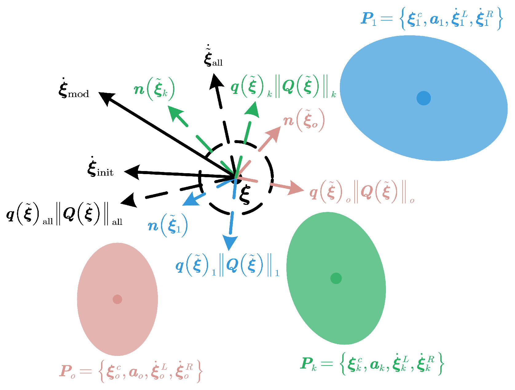
4.1. Real-Time End-Effector Adaptation

In this paper, we assume O convex obstacles around the robotic arm. Movement adaptation for the end-effector is achieved in Cartesian space by modulating the 3D positions while keeping the original orientations. Consider a state variable $\mathit{\xi }\in {\mathbb{R}}^3$ denoting the end effector 3D positions; its temporal dynamics is governed by an autonomous (time-invariant) and continuous function $f\left(\mathit{\xi }\right)$ as follows:

$$\dot{\mathit{\xi }}=\mathit{f}\left(\mathit{\xi }\right),\mathit{f}:{\mathbb{R}}^3\mapsto {\mathbb{R}}^3$$

(33)

Given the initial state ${\mathit{\xi }}_0$, the trajectory can be iteratively computed by integrating $f\left(\mathit{\xi }\right)$ according to:

$${\mathit{\xi }}_t={\mathit{\xi }}_{t-1}+\mathit{f}\left({\mathit{\xi }}_{t-1}\right)dt$$

(34)

where t is a positive integer and $dt$ is the integration time step.

For each obstacle $k\left(k=1\dots O\right)$, we define a distance function $\mathsf{\Gamma }\left({\mathit{\xi }}_k\right)$ with a continuous first-order partial derivative and monotonically increasing value away from the obstacle center ${\mathit{\xi }}_k^c$ to distinguish the space around an obstacle into three regions:

$$\begin{array}{c}\hfill \mathrm{Exterior}\mathrm{points}:{\mathcal{H}}^e=\left\{{\mathit{\xi }}_k\in {\mathbb{R}}^3:\mathsf{\Gamma }\left({\mathit{\xi }}_k\right)>1\right\}\\ \hfill \mathrm{Boundary}\mathrm{points}:{\mathcal{H}}^b=\left\{{\mathit{\xi }}_k\in {\mathbb{R}}^3:\mathsf{\Gamma }\left({\mathit{\xi }}_k\right)=1\right\}\\ \hfill \mathrm{Interior}\mathrm{points}:{\mathcal{H}}^i=\left\{{\mathit{\xi }}_k\in {\mathbb{R}}^3:\mathsf{\Gamma }\left({\mathit{\xi }}_k\right)<1\right\}\end{array}$$

(35)

To envelop obstacles, we construct the ellipsoid-shaped function $\mathsf{\Gamma }\left({\mathit{\xi }}_k\right)$ as follows:

$$\mathsf{\Gamma }\left({\mathit{\xi }}_k\right)=\sum _{i=1}^3{\left(\parallel {\mathit{\xi }}_k-{\mathit{\xi }}_k^c\parallel /a_i\right)}^{2p_i^k}$$

(36)

where $a_i$ is the i-th axis length and $p_i^k$ is a positive curvature parameter.

As shown in Figure 2, we parametrize the k-th obstacle (static or moving) as a vector ${\mathit{P}}_k=\left\{{\mathit{\xi }}_k^c,{\mathit{a}}_k,{\dot{\mathit{\xi }}}_k^L,{\dot{\mathit{\xi }}}_k^R\right\}$, where ${\mathit{a}}_k$ is the axis length, ${\dot{\mathit{\xi }}}_k^L$ and ${\dot{\mathit{\xi }}}_k^R$ are the linear and angular velocity with respect to the center ${\mathit{\xi }}_k^c$. Note that the static obstacle is a special case where the angular and linear velocities equal 0. Real-time obstacle avoidance for the end effector is achieved via a dynamic modulation matrix $\mathit{M}\left({\mathit{\xi }}_k\right)\in {\mathbb{R}}^{3\times 3}$ given that the local modulation matrix will not bring in new extrema with a cheap computational cost and closed-form solution [44]. To be generic, we derive the modulated trajectory from the original dynamics system (DS) in Equation (33) as follows:

$${\dot{\mathit{\xi }}}_k=\mathit{M}\left({\mathit{\xi }}_k\right)\left(\mathit{f}\left({\mathit{\xi }}_k\right)-{\dot{\tilde{\mathit{\xi }}}}_k\right)+{\dot{\tilde{\mathit{\xi }}}}_k\mathrm{with}{\dot{\tilde{\mathit{\xi }}}}_k={\dot{\mathit{\xi }}}_k^L+{\dot{\mathit{\xi }}}_k^R\times \left(\mathit{\xi }-{\mathit{\xi }}_k^c\right)$$

(37)

where ${\dot{\tilde{\mathit{\xi }}}}_k$ denotes the relative velocity induced by the obstacle motion. The modulation matrix $\mathit{M}\left({\mathit{\xi }}_k\right)$ is composed of the orthogonal basis matrix $\mathit{E}\left({\mathit{\xi }}_k\right)$ and the corresponding eigenvalue matrix $\mathit{D}\left({\mathit{\xi }}_k\right)$ as follows:

$$\mathit{M}\left({\mathit{\xi }}_k\right)=\mathit{E}\left({\mathit{\xi }}_k\right)\mathit{D}\left({\mathit{\xi }}_k\right)\mathit{E}{\left({\mathit{\xi }}_k\right)}^{-1}$$

(38)

For notational brevity, we define the relative position to the obstacle center ${\tilde{\mathit{\xi }}}_k=\mathit{\xi }-{\mathit{\xi }}_k^c$. Based on Equation (36), we derive the deflection hyperplane at point $\mathit{\xi }$ with the normal vector $\mathit{n}\left({\tilde{\mathit{\xi }}}_k\right)$ denoted as the distance function gradient $d\mathsf{\Gamma }\left(\mathit{\xi }\right)/d\mathit{\xi }$:

$$\mathit{n}\left({\tilde{\mathit{\xi }}}_k\right)={\left[{\displaystyle \frac{\partial {\mathsf{\Gamma }}_k\left({\tilde{\mathit{\xi }}}_k\right)}{\partial {\left(\mathit{\xi }\right)}_1}},{\displaystyle \frac{\partial {\mathsf{\Gamma }}_k\left({\tilde{\mathit{\xi }}}_k\right)}{\partial {\left(\mathit{\xi }\right)}_2}},{\displaystyle \frac{\partial {\mathsf{\Gamma }}_k\left({\tilde{\mathit{\xi }}}_k\right)}{\partial {\left(\mathit{\xi }\right)}_3}}\right]}^T$$

(39)

Given the normal vector, we formulate the basis matrix as follows:

$$\mathit{E}\left({\mathit{\xi }}_k\right)=\left[\mathit{n}\left({\tilde{\mathit{\xi }}}_k\right),{\mathit{e}}_1\left({\tilde{\mathit{\xi }}}_k\right),{\mathit{e}}_2\left({\tilde{\mathit{\xi }}}_k\right)\right]$$

(40)

where the tangent vectors are orthonormal to the normal as follows:

$$\begin{array}{c}\hfill \left\{\begin{array}{cc}{\mathit{e}}_1\left({\tilde{\mathit{\xi }}}_k\right)=\hfill & \left[-\mathit{n}{\left({\tilde{\mathit{\xi }}}_k\right)}_2,\mathit{n}{\left({\tilde{\mathit{\xi }}}_k\right)}_1,0\right]\hfill \\ {\mathit{e}}_2\left({\tilde{\mathit{\xi }}}_k\right)=\hfill & \mathit{n}\left({\tilde{\mathit{\xi }}}_k\right)\times {\mathit{e}}_1\left({\tilde{\mathit{\xi }}}_k\right)\hfill \end{array}\right.\end{array}$$

(41)

We define the related diagonal eigenvalue matrix $\mathit{D}\left({\mathit{\xi }}_k\right)$ to modify the normal and tangent directions independently with eigenvalues. The normal eigenvalue is selected to ensure impenetrability, that is, the eigenvalues should be zero on the obstacle surface. Meanwhile, the tangent eigenvalue should have the same magnitude in each direction to increase the velocity for moving around the obstacle. We formulate $\mathit{D}\left({\mathit{\xi }}_k\right)$ as follows:

$$\mathit{D}\left({\mathit{\xi }}_k\right)=\mathit{diag}\left({\lambda }_{\mathit{n}}\left({\mathit{\xi }}_k\right),{\lambda }_{\mathit{e}}\left({\mathit{\xi }}_k\right),{\lambda }_{\mathit{e}}\left({\mathit{\xi }}_k\right)\right)$$

(42)

Considering the safety margin, reactivity, and tail-effect in [30], we define the eigenvalue as follows:

$$\begin{array}{c}\hfill \left\{\begin{array}{cc}{\lambda }_{\mathit{n}}\left({\mathit{\xi }}_k\right)\hfill & =\left\{\begin{array}{cc}1-{\displaystyle \frac{1}{{\left|\mathsf{\Gamma }\left({\mathit{\xi }}_k\right)\right|}^{\frac{1}{{\rho }_k}}}}\hfill & \mathit{n}{\left({\tilde{\mathit{\xi }}}_k/{\eta }_k\right)}^T{\dot{\mathit{\xi }}}_k<0\hfill \\ 1\hfill & \mathit{n}{\left({\tilde{\mathit{\xi }}}_k/{\eta }_k\right)}^T{\dot{\mathit{\xi }}}_k⩾0\hfill \end{array}\right.\hfill \\ {\lambda }_{\mathit{e}}\left({\mathit{\xi }}_k\right)\hfill & =1+{\displaystyle \frac{1}{{\left|\mathsf{\Gamma }\left({\mathit{\xi }}_k\right)\right|}^{\frac{1}{{\rho }_k}}}}\hfill \end{array}\right.\end{array}$$

(43)

where ${\eta }_k$ is the safety magnitude for each direction, and ${\rho }_k$ is the reactivity parameter to determine the velocity modulation amplitude, that is, the larger the ${\rho }_k$, the earlier a robot reacts to the obstacle. To remedy the tail-effect, we check $\mathit{n}{\left({\tilde{\mathit{\xi }}}_k/{\eta }_k\right)}^T{\dot{\mathit{\xi }}}_k$ to evaluate whether the end effector is moving towards (negative) or away (positive) from the obstacle.

When it extends to multiple obstacles, as in Figure 2, we encapsulate all obstacles to create a single virtual obstacle by the weighted mean of each modulated DS in Equation (37). The benefit is that we only need to apply modulation once to ensure collision avoidance. Considering the impenetrability of the O obstacles and that the influence from other obstacles vanishes when approaching one obstacle boundary, we set the weight inversely proportional to the distance measure $\left(\mathsf{\Gamma }\left({\mathit{\xi }}_k\right)-1\right)$ as follows:

$${\mathit{w}}_k\left({\mathit{\xi }}_k\right)=\prod _{k=1,k\ne i}^O{\displaystyle \frac{\left(\mathsf{\Gamma }\left({\mathit{\xi }}_k\right)-1\right)}{\left(\mathsf{\Gamma }\left({\mathit{\xi }}_k\right)-1\right)+\left(\mathsf{\Gamma }\left({\mathit{\xi }}_i\right)-1\right)}}$$

(44)

Given Equations (33) and (37), to integrate O obstacles, for simplicity, we first compute the weighted mean of the relative velocity induced by the obstacle motion as follows:

$${\dot{\tilde{\mathit{\xi }}}}_{\mathrm{all}}=\sum _{k=1}^{O}exp\left(-{\displaystyle \frac{1}{{\rho }_k}}\left(\mathsf{\Gamma }\left({\mathit{\xi }}_k\right)-1\right)\right){\mathit{w}}_k\left({\mathit{\xi }}_k\right)\left({\dot{\mathit{\xi }}}_k^L+{\dot{\mathit{\xi }}}_k^R\times \left({\tilde{\mathit{\xi }}}_k/{\eta }_k\right)\right)$$

(45)

where we add the weight term ${\mathit{w}}_k^{\mathrm{rel}}=exp\left(-{\displaystyle \frac{1}{{\rho }_k}}\left(\mathsf{\Gamma }\left({\mathit{\xi }}_k\right)-1\right)\right)$ to smooth the distance influence.

In this paper, the combined weighted mean of $\mathit{f}\left({\mathit{\xi }}_k\right)$ refers to the init velocity ${\dot{\mathit{\xi }}}_{\mathrm{init}}$ computed from the offline task execution trajectory (see Section 3.3.2) with position differencing. To be specific, ${\dot{\mathit{\xi }}}_{\mathrm{init}}$ is a nonlinear function of $\mathit{\xi }$, which can be computed from the trajectory generalization method presented in Section 2.1 given the current position $\mathit{\xi }$. We further simplify Equation (37) as follows:

$$\begin{array}{cc}\hfill {\dot{\mathit{\xi }}}_{\mathrm{mod}}=& \mathit{M}{\left(\tilde{\mathit{\xi }}\right)}_{\mathrm{all}}\left({\dot{\mathit{\xi }}}_{\mathrm{init}}-{\dot{\tilde{\mathit{\xi }}}}_{\mathrm{all}}\right)+{\dot{\tilde{\mathit{\xi }}}}_{\mathrm{all}}\hfill \\ \hfill =& \mathit{q}{\left(\tilde{\mathit{\xi }}\right)}_{\mathrm{all}}{\parallel \mathit{Q}\left(\tilde{\mathit{\xi }}\right)\parallel }_{\mathrm{all}}+{\dot{\tilde{\mathit{\xi }}}}_{\mathrm{all}}\hfill \end{array}$$

(46)

where ${\parallel \mathit{Q}\left(\tilde{\mathit{\xi }}\right)\parallel }_{\mathrm{all}}$ and $\mathit{q}{\left(\tilde{\mathit{\xi }}\right)}_{\mathrm{all}}$ represent the combined magnitude and direction of $\mathit{M}{\left(\tilde{\mathit{\xi }}\right)}_{\mathrm{all}}\left({\dot{\mathit{\xi }}}_{\mathrm{init}}-{\dot{\tilde{\mathit{\xi }}}}_{\mathrm{all}}\right)$.

For the magnitude, given separate equivalent magnitude ${\parallel \mathit{Q}\left(\tilde{\mathit{\xi }}\right)\parallel }_k$ for each obstacle from Equation (37) and the weight in Equation (44), we can obtain:

$${\parallel \mathit{Q}\left(\tilde{\mathit{\xi }}\right)\parallel }_{\mathrm{all}}=\sum _{k=1}^O{\mathit{w}}_k\left({\mathit{\xi }}_k\right){\parallel \mathit{Q}\left(\tilde{\mathit{\xi }}\right)\parallel }_k$$

(47)

where ${\parallel \mathit{Q}\left(\tilde{\mathit{\xi }}\right)\parallel }_k$ is obtained from Equation (37):

$$\mathit{M}\left({\mathit{\xi }}_k\right)\left(\mathit{f}\left({\mathit{\xi }}_k\right)-{\dot{\tilde{\mathit{\xi }}}}_k\right)=\mathit{q}{\left(\tilde{\mathit{\xi }}\right)}_k{\parallel \mathit{Q}\left(\tilde{\mathit{\xi }}\right)\parallel }_k$$

(48)

Concerning the combined directions, given each equivalent directions $\mathit{q}{\left(\tilde{\mathit{\xi }}\right)}_k$, as [31], we define the function $\mathit{\kappa }\in {\mathbb{R}}^2$ to project the 3D original space onto a 2D hyper-sphere $\mathit{\kappa }$ space with radius $\pi$ as follows:

$$\mathit{\kappa }\left({\dot{\mathit{\xi }}}_k,\tilde{\mathit{\xi }}\right)=\mathrm{arc}cos\left({\widehat{\mathit{q}}}_1^{{\dot{\mathit{\xi }}}_k}\right){\displaystyle \frac{\left[{\widehat{\mathit{q}}}_2^{{\dot{\mathit{\xi }}}_k},{\widehat{\mathit{q}}}_3^{{\dot{\mathit{\xi }}}_k}\right]}{{\widehat{\mathit{q}}}_2^{{\dot{\mathit{\xi }}}_k}+{\widehat{\mathit{q}}}_3^{{\dot{\mathit{\xi }}}_k}}},{\widehat{\mathit{q}}}^{{\dot{\mathit{\xi }}}_k}={\mathit{R}}_{\mathit{f}}^T\mathit{q}{\left(\tilde{\mathit{\xi }}\right)}_k$$

(49)

where ${\mathit{R}}_{\mathit{f}}$ is the projection matrix formulated from the unit vector ${\mathit{n}}^f\left(\mathit{\xi }\right)$ for the init vel ${\dot{\mathit{\xi }}}_{\mathrm{init}}$ along with two orthonormal bases ${\mathit{e}}_1^f\left(\mathit{\xi }\right),{\mathit{e}}_2^f\left(\mathit{\xi }\right)$:

$${\mathit{R}}_f\left(\mathit{\xi }\right)=\left[{\mathit{n}}^f\left(\mathit{\xi }\right),{\mathit{e}}_1^f\left(\mathit{\xi }\right),{\mathit{e}}_2^f\left(\mathit{\xi }\right)\right]$$

(50)

We then evaluate the weighted mean in this $\mathit{\kappa }$ space as follows:

$$\mathit{\kappa }{\left(\mathit{\xi }\right)}_{\mathrm{all}}=\sum _{k=1}^O{\mathit{w}}_k\left({\mathit{\xi }}_k\right)\mathit{\kappa }\left({\dot{\mathit{\xi }}}_k,\tilde{\mathit{\xi }}\right)$$

(51)

with the combined direction $\mathit{q}{\left(\mathit{\xi }\right)}_{\mathrm{all}}$ expressed back to the original 3D space as follows:

$$\mathit{q}{\left(\mathit{\xi }\right)}_{\mathrm{all}}={\mathit{R}}_f\left(\mathit{\xi }\right){\left[cos\parallel \mathit{\kappa }{\left(\mathit{\xi }\right)}_{\mathrm{all}}\parallel ,{\displaystyle \frac{sin\parallel \mathit{\kappa }{\left(\mathit{\xi }\right)}_{\mathrm{all}}\parallel }{\parallel \mathit{\kappa }{\left(\mathit{\xi }\right)}_{\mathrm{all}}\parallel }}\parallel \mathit{\kappa }{\left(\mathit{\xi }\right)}_{\mathrm{all}}\parallel \right]}^T$$

(52)

The final modulated velocity and position for the O obstacles can be computed with Equation (46) and velocity integration (Equation (34)). To sum up, the complete real-time robot end effector adaptation method comprises the following steps: First, we obtain the initial task execution trajectory with T timesteps and $dt$ integration steps after the offline optimization and adaptation procedure in Section 3.3.2. Given the initial velocity at $t=0$ with position differencing, the modulated velocity is computed from Equation (46) with the presence of dynamic obstacles. We then apply velocity integration (Equation (34)) to obtain the expected position for the next timestep. The offline trajectory beyond the current timestep is treated as a template trajectory. Given the current position and the changing target point, we utilize the proposed trajectory generalization method in Section 2.1 to generate the remaining trajectory and compute the velocity via position differencing. The velocity is treated as the initial velocity at the next timestep, and we apply modulation iteratively to obtain the whole modulated trajectory with the expected velocity for the robot end-effector. Note that if the modulated positons collide, we treat them as init positions and modulate them iteratively until safe.

During the real-time end-effector modulation process, we leverage the demonstration information from the offline optimization phase through trajectory generalization, preserving the human demonstration characteristics. The initial velocity at the next timestep is determined based on the generalized trajectory, rather than being arbitrarily chosen, which integrates offline optimization and online modulation. The end-effector modulation provides the modulated velocity and the desired position at each timestep, which are utilized for subsequent real-time non-end-effector adaptation.

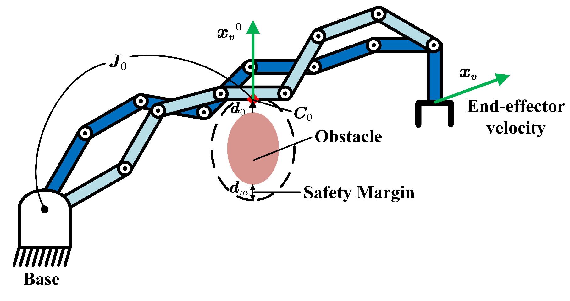
4.2. Real-Time Non-End-Effector Adaptation

We ensure real-time obstacle avoidance for the robot end effector in Section 4.1; however, the potential collisions between other robot links (non-end-effector) and obstacles are not considered. To achieve real-time non-end-effector adaptation, given the expected velocity in Cartesian space, we utilize the robot joint redundancy with null-space velocity control. In particular, the 7-DoF manipulator is considered in this paper; its end effector velocity ${\mathit{x}}_{\mathit{v}}$ and joint velocity ${\mathit{q}}_{\mathit{v}}$ conform to:

$${\mathit{x}}_{\mathit{v}}={\mathit{Jq}}_{\mathit{v}}$$

(53)

where $\mathit{J}$ is a $6\times 7$ Jacobian matrix. Considering $\mathit{J}$ is not a square matrix, given the expected end-effector velocity ${\mathit{x}}_{\mathit{v}}$, the joint velocity ${\mathit{q}}_{\mathit{v}}$ is derived by:

$${\mathit{q}}_{\mathit{v}}={\mathit{J}}^{\#}{\mathit{x}}_{\mathit{v}}+\mathit{N}{\delta }_{\mathit{v}}$$

(54)

where ${\mathit{J}}^{\#}$ is the generalized inverse and $\mathit{N}$ is the null space matrix of $\mathit{J}$; that is, whatever the value of the 7-dimensional joint velocity vector ${\delta }_{\mathit{v}}$, the resulted end-effector velocity $\mathit{N}{\delta }_{\mathit{v}}$ remains 0. To derive ${\mathit{J}}^{\#}$, we minimize the norm error between ${\mathit{J}}^{\#}{\mathit{x}}_{\mathit{v}}$ and ${\mathit{q}}_{\mathit{v}}$ with the least square solution ${\mathit{J}}^{+}={\mathit{J}}^T{\left({\mathit{JJ}}^T\right)}^{-1}$ satisfying the Moor–Penrose inverse [45]. We rewrite Equation (54) with ${\mathit{J}}^{+}$ as follows:

$${\mathit{q}}_{\mathit{v}}={\mathit{J}}^{+}{\mathit{x}}_{\mathit{v}}+\left(\mathit{I}-{\mathit{J}}^{+}\mathit{J}\right){\delta }_{\mathit{v}}$$

(55)

The term $\left(\mathit{I}-{\mathit{J}}^{+}\mathit{J}\right){\delta }_{\mathit{v}}$ provides distinct joint velocity configurations resulting in the same end-effector velocity.

Considering multiple solutions for the joint velocity vector ${\delta }_{\mathit{v}}$ in Equation (54), we aim to ensure that ${\delta }_{\mathit{v}}$ retains the joint velocity distributions of the 7DoF ProMPs during offline optimization while minimizing the norm error between ${\mathit{J}}^{\#}{\mathit{x}}_{\mathit{v}}$ and ${\mathit{q}}_{\mathit{v}}$ in Equation (54). This allows us to integrate offline task-constrained optimization and real-time movement adaptation for robot whole-body control with Joint ProMPs. To derive the joint veloicty distributions, at the current time step t, the mean ${{\mathit{\mu }}_{{\mathit{q}}_{\mathit{v}}}}^t$ and standard deviation ${{\mathit{\sigma }}_{{\mathit{q}}_{\mathit{v}}}}^t$ of the joint velocities are computed based on the joint positions and are expressed in the form of ProMPs basis functions as follows:

$$\begin{array}{c}\hfill {{\mathit{\mu }}_{{\mathit{q}}_{\mathit{v}}}}^t={\displaystyle \frac{1}{dt}}\ast \left({{\mathit{\mu }}_{\mathit{q}}}^{t+1}-{{\mathit{\mu }}_{\mathit{q}}}^t\right)\\ \hfill {{\mathit{\sigma }}_{{\mathit{q}}_{\mathit{v}}}}^t={\displaystyle \frac{1}{d{t}^2}}\ast \left({{\mathit{\sigma }}_{\mathit{q}}}^{t+1}+{{\mathit{\sigma }}_{\mathit{q}}}^t\right)\end{array}$$

(56)

where

$$\begin{array}{c}\hfill {{\mathit{\mu }}_{\mathit{q}}}^{t+1}={\mathbf{\Psi }}_{t+1}^T{{\mathit{\mu }}_{\mathit{w}}}^{*},{{\mathit{\mu }}_{\mathit{q}}}^t={\mathbf{\Psi }}_t^T{{\mathit{\mu }}_{\mathit{w}}}^{*}\\ \hfill {{\mathit{\sigma }}_{\mathit{q}}}^{t+1}={\mathbf{\Psi }}_{t+1}^T{{\mathbf{\Sigma }}_{\mathit{w}}}^{*},{{\mathit{\sigma }}_{\mathit{q}}}^t={\mathbf{\Psi }}_t^T{{\mathbf{\Sigma }}_{\mathit{w}}}^{*}\end{array}$$

(57)

where $\left({{\mathit{\mu }}_{\mathit{q}}}^t,{{\mathit{\sigma }}_{\mathit{q}}}^t\right)$ represents the optimized mean and standard deviation of the joint positions with $\left({{\mathit{\mu }}_{\mathit{w}}}^{*},{{\mathbf{\Sigma }}_{\mathit{w}}}^{*}\right)$ denoting the optimized mean and covariance matrix of the 7DoF Joint ProMPs. To simplify the notation, we omit the superscript ^t. Given that the modulation is performed at each timestep, the mean and standard deviation of the joint velocities at each timestep are expressed with ${\mathit{\mu }}_{{\mathit{q}}_{\mathit{v}}}$ and ${\mathit{\sigma }}_{{\mathit{q}}_{\mathit{v}}}$.

To minimize the norm $∥{\mathit{q}}_{\mathit{v}}-{\mathit{J}}^{\#}{\mathit{x}}_{\mathit{v}}∥$ in Equation (54), while ensuring that the resulting joint velocity vector adheres to the optimized distribution at each time step, we define the loss function $L\left({\delta }_{\mathit{v}}\right)$ as follows:

$$L\left({\delta }_{\mathit{v}}\right)={\Vert {\mathit{q}}_{\mathit{v}}-{\mathit{J}}^{\#}{\mathit{x}}_{\mathit{v}}\Vert }^2+\lambda \sum _{i=1}^7{\left({\displaystyle \frac{({{\mathit{q}}_{\mathit{v}}}^i-{{\mathit{\mu }}_{{\mathit{q}}_{\mathit{v}}}}^i)}{{{\mathit{\sigma }}_{{\mathit{q}}_{\mathit{v}}}}^i}}\right)}^2$$

(58)

We further substitute Equation (54) into the above equation to obtain:

$$L\left({\delta }_{\mathit{v}}\right)={∥\mathit{N}{\delta }_{\mathit{v}}∥}^2+\lambda \sum _{i=1}^7{\left({\displaystyle \frac{{\left(\mathit{N}{\delta }_{\mathit{v}}+{\mathit{J}}^{\#}{\mathit{x}}_{\mathit{v}}-{\mathit{\mu }}_{{\mathit{q}}_{\mathit{v}}}\right)}^i}{{{\mathit{\sigma }}_{{\mathit{q}}_{\mathit{v}}}}^i}}\right)}^2$$

(59)

where $\lambda$ is the regularization term. By minimizing $L\left({\delta }_{\mathit{v}}\right)$ with respect to ${\delta }_{\mathit{v}}$, we obtain the joint velocity vector as follows:

$${\delta }_{\mathit{v}}={\left({\mathit{N}}^T\mathit{N}+\lambda {\mathit{N}}^T{{\mathbf{\Sigma }}_{{\mathit{q}}_{\mathit{v}}}}^{-1}\mathit{N}\right)}^{-1}{\mathit{N}}^T\left({\mathit{\mu }}_{{\mathit{q}}_{\mathit{v}}}-{\mathit{J}}^{\#}{\mathit{x}}_{\mathit{v}}\right)$$

(60)

where ${\mathbf{\Sigma }}_{{\mathit{q}}_{\mathit{v}}}=\mathrm{diag}{\left([{{\mathit{\sigma }}_{{\mathit{q}}_{\mathit{v}}}}^1,{{\mathit{\sigma }}_{{\mathit{q}}_{\mathit{v}}}}^2,\dots ,{{\mathit{\sigma }}_{{\mathit{q}}_{\mathit{v}}}}^7]\right)}^2$ represents the diagonal covariance matrix composed of the standard deviations ${\mathit{\sigma }}_{{\mathit{q}}_{\mathit{v}}}$ for the offline-optimized 7DoF joint velocities.

In addition to preserving the joint distribution, we also need to perform real-time collision detection between the robot’s links and obstacles with dynamic modulation to achieve null-space velocity control. Figure 3 demonstrates the null space velocity control strategy. We detect the closest point on the robot non-end-effector to each obstacle and enforce velocity ${\mathit{x}}_{\mathit{v}}^0$ at that point if the point is within the obstacle safety margin ${\mathit{d}}_m$. The vector ${\mathit{d}}_0$ starts from the obstacle surface to the point $C_0$, with the same direction as ${\mathit{x}}_{\mathit{v}}^0$, and ${\mathit{J}}_0$ is the Jacobian matrix from the base to point $C_0$. We further denote the end-effector velocity ${\mathit{x}}_{\mathit{v}}$ and the point $C_0$ velocity ${\mathit{x}}_{\mathit{v}}^0$ with Equation (53):

$${\mathit{x}}_{\mathit{v}}={\mathit{Jq}}_{\mathit{v}},{\mathit{x}}_{\mathit{v}}^0={\mathit{J}}_0{\mathit{q}}_{\mathit{v}}$$

(61)

We substitute Equation (54) to ${\mathit{x}}_{\mathit{v}}^0={\mathit{J}}_0{\mathit{q}}_{\mathit{v}}$ with ${\delta }_{\mathit{v}}$ derived as folllows:

$${\delta }_{\mathit{v}}={\left({\mathit{J}}_{\mathbf{0}}\mathit{N}\right)}^{\#}\left({\mathit{x}}_{\mathit{v}}^0-{\mathit{J}}_{\mathbf{0}}{\mathit{J}}^{\#}{\mathit{x}}_{\mathit{v}}\right)$$

(62)

To achieve a trade-off between maintaining consistency with the optimized distribution and ensuring a safe distance from the robot non-end-effector, we define the coefficients $\gamma >0$ and $\rho >0$ satisfying $\gamma +\rho =1$. We weight the joint velocity vectors from Equations (60) and (62) to obtain the combined joint velocity vector ${{\delta }_{\mathit{v}}}^{*}$ as follows:

$${{\delta }_{\mathit{v}}}^{*}=\gamma {\left({\mathit{N}}^T\mathit{N}+\lambda {\mathit{N}}^T{{\mathbf{\Sigma }}_{{\mathit{q}}_{\mathit{v}}}}^{-1}\mathit{N}\right)}^{-1}{\mathit{N}}^T\left({\mathit{\mu }}_{{\mathit{q}}_{\mathit{v}}}-{\mathit{J}}^{\#}{\mathit{x}}_{\mathit{v}}\right)+\rho {\left({\mathit{J}}_0\mathit{N}\right)}^{\#}\left({\mathit{x}}_{\mathit{v}}^0-{\mathit{J}}_0{\mathit{J}}^{\#}{\mathit{x}}_{\mathit{v}}\right)$$

(63)

Taking $\dot{\mathit{q}}$ and $\dot{\mathit{x}}$ as control variables and substituting Equation (63) to $\dot{\mathit{q}}={\mathit{J}}^{\#}\dot{\mathit{x}}+{\mathit{N}{\delta }_{\mathit{v}}}^{*}$, we obtain:

$$\dot{\mathit{q}}={\mathit{J}}^{\#}\dot{\mathit{x}}+\gamma \mathit{N}{\left({\mathit{N}}^T\mathit{N}+\lambda {\mathit{N}}^T{{\mathbf{\Sigma }}_{{\mathit{q}}_{\mathit{v}}}}^{-1}\mathit{N}\right)}^{-1}{\mathit{N}}^T\left({\mathit{\mu }}_{{\mathit{q}}_{\mathit{v}}}-{\mathit{J}}^{\#}{\mathit{x}}_{\mathit{v}}\right)+\rho \mathit{N}{\left({\mathit{J}}_0\mathit{N}\right)}^{\#}\left({\mathit{x}}_{\mathit{v}}^0-{\mathit{J}}_0{\mathit{J}}^{\#}{\mathit{x}}_{\mathit{v}}\right)$$

(64)

Due to the idempotent and hermitian nature of $\mathit{N}=\mathit{I}-{\mathit{J}}^{+}\mathit{J}$ in Equation (55), that is, ${\left({\mathit{J}}_{\mathbf{0}}\mathit{N}\right)}^{\#}=\mathit{N}{\left({\mathit{J}}_{\mathbf{0}}\mathit{N}\right)}^{\#}$, we simplify Equation (64) as follows:

$$\dot{\mathit{q}}={\mathit{J}}^{\#}\dot{\mathit{x}}+\gamma \mathit{N}{\left({\mathit{N}}^T\mathit{N}+\lambda {\mathit{N}}^T{{\mathbf{\Sigma }}_{{\mathit{q}}_{\mathit{v}}}}^{-1}\mathit{N}\right)}^{-1}{\mathit{N}}^T\left({\mathit{\mu }}_{{\mathit{q}}_{\mathit{v}}}-{\mathit{J}}^{\#}{\mathit{x}}_{\mathit{v}}\right)+\rho {\left({\mathit{J}}_0\mathit{N}\right)}^{\#}\left({\mathit{x}}_{\mathit{v}}^0-{\mathit{J}}_0{\mathit{J}}^{\#}{\mathit{x}}_{\mathit{v}}\right)$$

(65)

Given the expected end-effector velocity ${\mathit{x}}_{\mathit{v}}$, we can utilize Equation (65) to design a feedback controller for non-end-effector adaptation. In this context, ${\mathit{J}}^{\#}\dot{\mathit{x}}$ is used to track ${\mathit{x}}_{\mathit{v}}$, ${\mathit{J}}_0{\mathit{J}}^{\#}{\mathit{x}}_{\mathit{v}}$ denote the point $C_0$ velocity attributed to ${\mathit{x}}_{\mathit{v}}$, and ${\left({\mathit{J}}_0\mathit{N}\right)}^{\#}$ is used to transform the Cartesian velocity ${\mathit{x}}_{\mathit{v}}^0-{\mathit{J}}_0{\mathit{J}}^{\#}{\mathit{x}}_{\mathit{v}}$ into the joint velocity. In this paper, considering the manipulator redundancy is 1, less than 3, we define the direction of ${\mathit{x}}_{\mathit{v}}^0$ the same as vector ${\mathit{d}}_0$ as ${\mathit{x}}_{\mathit{v}}^0=v_0{\mathit{n}}_0,{\mathit{n}}_0={\displaystyle \frac{{\mathit{d}}_0}{\parallel {\mathit{d}}_0\parallel }}$, where ${\mathit{n}}_0$ is the unit vector of ${\mathit{d}}_0$, and $v_0$ is a scalar velocity. To obtain smooth and flexible motion for obstacle avoidance, we define $v_0$ as in Equation (66), where ${\mathit{d}}_m$ is the safety margin, and ${\mathit{d}}_n$ denotes the distance at which the obstacle begins to affect the manipulator to construct a smoothing factor $(1+cos\left(\pi {\displaystyle \frac{\parallel {\mathit{d}}_0\parallel -{\mathit{d}}_m}{{\mathit{d}}_n-{\mathit{d}}_m}}\right))$.

$$\begin{array}{c}\hfill \left\{\begin{array}{cc}{v}_0\hfill & ={\lambda }_v{v}_n\hfill \\ {\lambda }_v\hfill & =\left\{\begin{array}{c}\begin{array}{ccc}\hfill & {\left({\displaystyle \frac{{\mathit{d}}_m}{\parallel {\mathit{d}}_0\parallel }}\right)}^2-1\hfill & \hfill \mathrm{if}\parallel {\mathit{d}}_0\parallel <{\mathit{d}}_m\\ \hfill & {\displaystyle \frac{1}{2}}\left(1+cos\left(\pi {\displaystyle \frac{\parallel {\mathit{d}}_0\parallel -{\mathit{d}}_m}{{\mathit{d}}_n-{\mathit{d}}_m}}\right)\right)\left({\left({\displaystyle \frac{{\mathit{d}}_m}{\parallel {\mathit{d}}_0\parallel }}\right)}^2-1\right)\hfill & \hfill \mathrm{if}{\mathit{d}}_m<\parallel {\mathit{d}}_0\parallel <{\mathit{d}}_n\\ \hfill & 0\hfill & \hfill \mathrm{if}\parallel {\mathit{d}}_0\parallel ⩾{\mathit{d}}_n\end{array}\hfill \end{array}\right.\hfill \end{array}\right.\end{array}$$

(66)

Let $\mathit{x}=T\left(\mathit{q}\right)$ denote the end effector pose obtained through the forward kinematics function $T\left(.\right)$; the expected end effector pose can be derived with velocity integration:

$${\mathit{x}}_d={\dot{\mathit{\xi }}}_{\mathrm{mod}}+{\dot{\mathit{\xi }}}_{\mathrm{mod}}dt={\mathit{x}}_{\mathit{v}}+{\mathit{x}}_{\mathit{v}}dt$$

(67)

we then express the feed-back controller error $\mathit{e}\left(\mathit{x}\right)$ as follows:

$$\mathit{e}\left(\mathit{x}\right)={\mathit{x}}_d-T\left(\mathit{q}\right)$$

(68)

and further denote the resulted joint gradient $d\mathit{q}$ as follows:

$$d\mathit{q}={\mathit{J}}^{\#}\mathit{e}\left(\mathit{x}\right)+\gamma \mathit{N}{\left({\mathit{N}}^T\mathit{N}+\lambda {\mathit{N}}^T{{\mathbf{\Sigma }}_{{\mathit{q}}_{\mathit{v}}}}^{-1}\mathit{N}\right)}^{-1}{\mathit{N}}^T\left({\mathit{\mu }}_{{\mathit{q}}_{\mathit{v}}}-{\mathit{J}}^{\#}{\mathit{x}}_{\mathit{v}}\right)+\rho {\left({\mathit{J}}_0\mathit{N}\right)}^{\#}\left({\mathit{x}}_{\mathit{v}}^0-{\mathit{J}}_0{\mathit{J}}^{\#}{\mathit{x}}_{\mathit{v}}\right)$$

(69)

We derive $\mathit{q}$ with integration $\mathit{q}=\mathit{q}+d\mathit{q}d\mathrm{t}$, and continue the iteration process until the error meets the stopping criterion to obtain the modulated joint positions ${\mathit{q}}_{\mathrm{mod}}$ for real-time task execution.

To integrate the offline and real-time robot movement adaptation methods presented in Section 3 and Section 4, we summarize the overall control framework in Figure 4.

Given an offline task execution trajectory ${\left\{\mathit{x},\mathit{y},\mathit{z},\mathit{o}\right\}}_{t=1}^T$ obtained from Algorithm 1, the initial velocity ${\dot{\mathit{\xi }}}_{\mathrm{init}}^t$ is computed using position differencing. In the presence of O dynamic obstacles, represented as ${\left\{{\mathit{\xi }}_k^c,{\mathit{a}}_k,{\dot{\mathit{\xi }}}_k^L,{\dot{\mathit{\xi }}}_k^R\right\}}_{k=1}^O$, we derive the modulation matrix $\mathit{M}\left({\mathit{\xi }}_k\right)\in {\mathbb{R}}^{3\times 3}$ and the weight coefficient ${\mathit{w}}_k\left({\mathit{\xi }}_k\right)$ for each obstacle. Additionally, we identify the closest point $C_0$ on the robot’s non-end-effector links and define the corresponding vector ${\mathit{d}}_0$. The avoidance velocity ${\mathit{x}}_{\mathit{v}}^0=v_0{\mathit{n}}_0,{\mathit{n}}_0={\displaystyle \frac{{\mathit{d}}_0}{\parallel {\mathit{d}}_0\parallel }}$ is then determined accordingly from Equation (66).

For online end-effector adaptation, we compute the equivalent modulation magnitude and direction for each obstacle, denoted as $\mathit{q}{\left(\tilde{\mathit{\xi }}\right)}_k{\parallel \mathit{Q}\left(\tilde{\mathit{\xi }}\right)\parallel }_k$. These are then combined using weighted summation with ${\mathit{w}}_k\left({\mathit{\xi }}_k\right)$, along with hyper-sphere projection $\mathit{\kappa }\in {\mathbb{R}}^2$, to obtain the overall modulation effect $\mathit{q}{\left(\tilde{\mathit{\xi }}\right)}_{\mathrm{all}}{\parallel \mathit{Q}\left(\tilde{\mathit{\xi }}\right)\parallel }_{\mathrm{all}}$. The resulting modulated velocity ${\dot{\mathit{\xi }}}_{\mathrm{mod}}$ serves as the desired end-effector velocity. The expected position ${\mathit{x}}_d$ at the next timestep is determined via velocity integration. Note that if ${\mathit{x}}_d$ collides, we treat it as the initial position and modulate it iteratively until safe.

For online non-end-effector adaptation, given the mean and diagonal covariance matrix $\left({\mathit{\mu }}_{{\mathit{q}}_{\mathit{v}}},{\mathbf{\Sigma }}_{{\mathit{q}}_{\mathit{v}}}\right)$ from offline optimization with 7DoF Joint ProMPs, along with the null-space velocity component, Equation (69) is constructed to design the control diagram. Given the expected position ${\mathit{x}}_d$, the system iterates through a control loop, minimizing the error defined in Equations (67)–(69) until the stopping criteria are met. If any joint configuration results in a collision, the nominal velocity norm $v_0$ is iteratively increased, and the control loop is repeated until a safe motion is achieved. The modulated joint positions ${\mathit{q}}_{\mathrm{mod}}$ are then used for real-time task execution. Furthermore, at each timestep, the initial velocity for the next step is estimated using trajectory generalization based on the current position ${\mathit{x}}_d$. This process repeats iteratively until all T timesteps are completed.

5. Experimental Validation

In this section, we validate the proposed human–robot skill transfer strategy within an industrial scenario where a robot learns different skills from the human to move around the obstacle and grasp the emergency stop. We first conduct human–robot skill transfer experiments. After the robot learns the skills, we evaluate our method in different static (offline) and dynamic (real-time) environments, and compare our method to other similar movement adaptation methods. For clarity, we summarize the definitions of all the parameters employed in the experiment section in

Table 1. Definitions of all parameters employed in the experiment section.

Offline Adaptation	Description
$f\left(\mathit{p}\right)$	Trajectory shape modulation for 3D positions
$R_{\mathrm{obs}}$	The obstacle radius
$\mathrm{X},\mathrm{Y},\mathrm{Z}$	The 3D position sets for via-points range
$\gamma$	The threshold for fine-tuning via-points
T	The forward kinematics function
$d_{k,t}$	The distance threshold to represent task constraints probability
${\mathit{n}}_{z,t},{\mathit{b}}_{z,t}$	The hyperplane normal and bias vectors for the maximum Z
$R_{\mathrm{obs}}$	The obstacle safe radius
${\alpha }_{k,t}$	The confidence level to represent the task constraints probability
${{\lambda }_{k,t}}^0$	The initial Lagrange multiplier
$p\left({\mathit{w}}^0\right)=\mathcal{N}\left({\mathit{w}}^0;{\mathit{\mu }}_{\mathit{w}}^0,{\mathbf{\Sigma }}_{\mathit{w}}^0\right)$	Initial Gaussian distributions of ProMPs
$p\left({\mathit{w}}^{*}\right)=\mathcal{N}\left({\mathit{w}}^{*};{\mathit{\mu }}_{\mathit{w}}^{*},{\mathbf{\Sigma }}_{\mathit{w}}^{*}\right)$	Optimized Gaussian distributions of ProMPs
$p\left({\mathit{q}}_t\right)=\mathcal{N}\left({\mathit{q}}_t;{\mathit{\mu }}_t^0,{\mathit{\sigma }}_t^0\right)$	The initial mean and standard deviation of each timestep
$p\left({\mathit{q}}_t\right)=\mathcal{N}\left({\mathit{q}}_t;{\mathit{\mu }}_t^{*},{\mathit{\sigma }}_t^{*}\right)$	The optimized mean and standard deviation of each timestep
${\mathit{q}}_t^{\mathrm{safe}}\in \left({\mathit{\mu }}_t^{*}-2{\mathit{\sigma }}_t^{*},{\mathit{\mu }}_t^{*}+2{\mathit{\sigma }}_t^{*}\right)$	The optimized joint limit range
${\mathbf{\Psi }}_t^T$	Gaussian basis functions
${\mathit{q}}_t^0={\mathbf{\Psi }}_t^T{\mathit{w}}^{*}$	The initial joint value for Jacobian IK
$dt$	The interval between adjacent timesteps
$\mathsf{\Gamma }\left({\mathit{\xi }}_k\right)$	The ellipsoid-shaped distance function
$p_i^k,{\mathit{\xi }}_k^c$	The curvature parameter and the center of the distance function
${\dot{\mathit{\xi }}}_k^L,{\dot{\mathit{\xi }}}_k^R$	The linear and angular velocities of dynamic obstacles
Real-Time Adaptation	Description
$\mathit{n}\left({\tilde{\mathit{\xi }}}_k\right)$	The normal vector of the deflection hyperplane at point $\mathit{\xi }$
$\mathit{E}\left({\mathit{\xi }}_k\right),\mathit{D}\left({\mathit{\xi }}_k\right)$	The basis and the diagonal eigenvalue matrix
${\eta }_k,{\rho }_k$	The safety magnitude and reactivity parameter for $\mathsf{\Gamma }\left({\mathit{\xi }}_k\right)$
$\mathit{n}{\left({\tilde{\mathit{\xi }}}_k/{\eta }_k\right)}^T{\dot{\mathit{\xi }}}_k$	Tail-effect definition for $\mathsf{\Gamma }\left({\mathit{\xi }}_k\right)$
$\mathit{M}\left({\mathit{\xi }}_k\right)\in {\mathbb{R}}^{3\times 3},{\mathit{w}}_k\left({\mathit{\xi }}_k\right)$	The modulation matrix and weighted coefficient for each dynamic obstacle
${\parallel \mathit{Q}\left(\tilde{\mathit{\xi }}\right)\parallel }_{\mathrm{all}},\mathit{q}{\left(\tilde{\mathit{\xi }}\right)}_{\mathrm{all}}$	The weighted magnitude and directions for all dynamic obstacles
${\dot{\mathit{\xi }}}_{\mathrm{init}},{\dot{\mathit{\xi }}}_{\mathrm{mod}}$	The initial and modulated velocity in Cartesian space
$C_0$	The closest point between the robot links and the obstacle
${\mathit{x}}_{\mathit{v}}^0,{\mathit{J}}_0$	The retreat velocity and the Jacobian matrix at point $C_0$
$\parallel {\mathit{d}}_0\parallel$	The minimum detected distance between robot links 1 to 6 and the obstacle
${\mathit{d}}_m$	The safety margin for dynamic obstacles
${\mathit{w}}_1^{\mathrm{rel}},{\dot{\tilde{\mathit{\xi }}}}_{\mathrm{all}}$	The weight term and weighted relative velocity
$\left\{{\mathit{\xi }}_{\mathrm{next}}\right\},{\dot{\mathit{\xi }}}_{\mathrm{next}}$	The next generalized trajectory sets and the next velocity computed
${\mathit{d}}_{\mathrm{n}}$	The distance at which the obstacle begins to affect the manipulator
$v_n$	The scalar velocity
${\mathit{q}}_{\mathrm{mod}}$	The modulated joint configuration

.

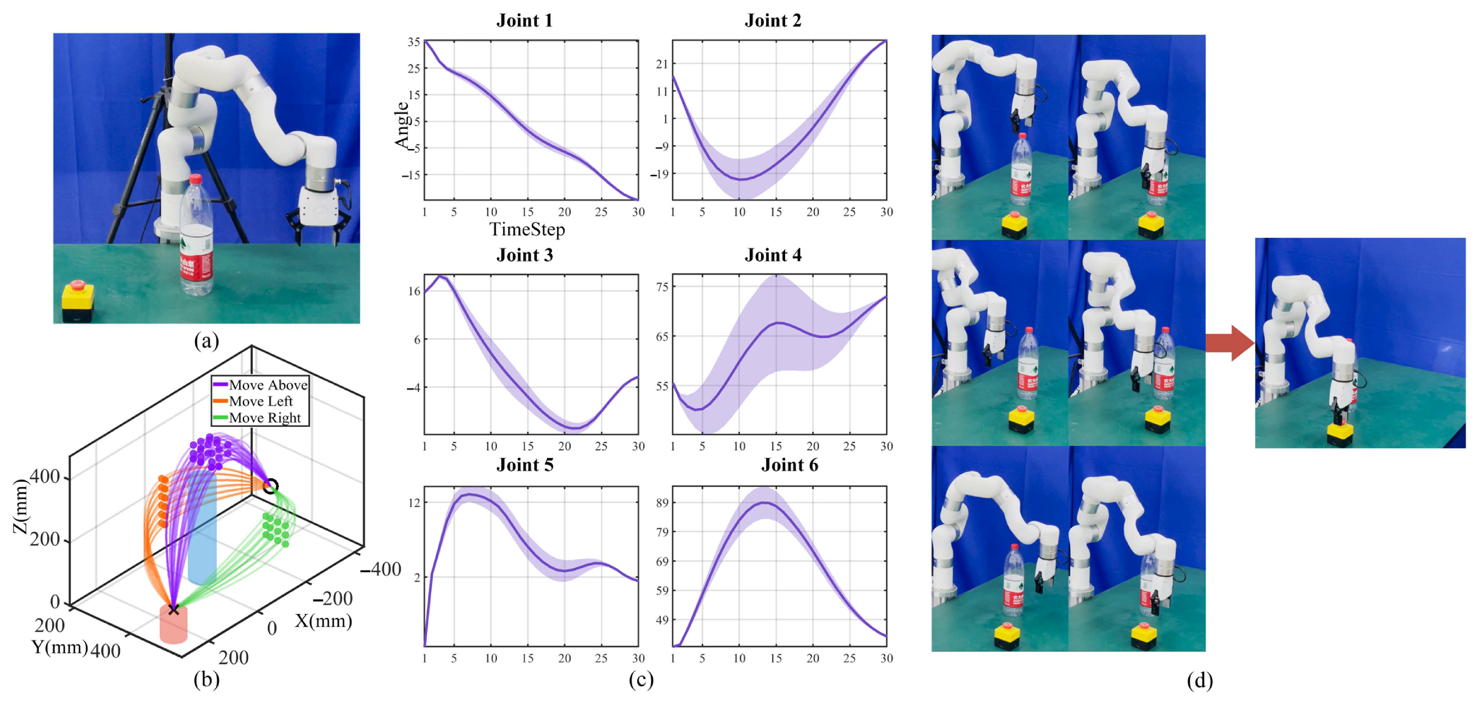
5.1. Template Trajectory Generalization from Only One Human Demonstration

The Ufactory Xarm 7-DoF manipulator is selected to validate our method. A Kinect V2 camera is positioned on the side to track continuous human hand movements, while a Zed2i binocular camera is mounted overhead to capture task-related object poses. For a single obstacle scenario, the robot is taught three distinct skills: moving above, left, and right around the obstacle using the Kinect FORTH system. Each skill is demonstrated only once, with the human hand centroid trajectories recorded (see Figure 5a). The Kinect FORTH system captures real-time 6D poses of the human hand centroid and provides a colored model of the fingers, enabling precise trajectory acquisition.

For each skill, the trajectory is smoothed using a Moving Average Filter (MAF), normalized to 30 timesteps, and transformed into the robot base frame. It is further converted to the table frame at the tabletop surface. Utilizing our trajectory generalization method (see Section 2.1), the trajectory is generalized with the same start and end points, without via-points, to generate the template trajectory for each skill (see Figure 5b). To account for the inherent noise in the Kinect FORTH system, the trajectories are aligned to the same start and end point, ensuring consistency for subsequent offline task optimization. A suitable start point is set, and the end point is determined based on the emergency stop 3D positions detected by YOLO [46]. The template trajectory corresponds to the minimum Z-position of the robot gripper center.

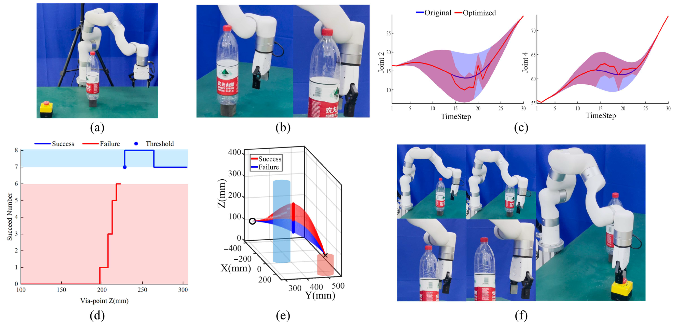
5.2. Offline Movement Adaptation

Given the template trajectory, we validate the offline task-constrained adaptation algorithm (Algorithm 1) under a static scene with the presence of a new big bottle, as shown in Figure 6a. We randomly place the emergency stop and the bottle with 3D positions detected by YOLO. For each skill, the robot first generates collision-free end-effector trajectory sets with via-point trajectory generalization (see Section 2.1). We select the feature via-points corresponding to the max norm of shape modulation $f\left(\mathit{p}\right)$ and set discrete via-points with equal spacing to construct the initial trajectory sets. To be specific, for the above skill, the X- and Y-positions are within the radius $R_{\mathrm{obs}}$ = 39 mm around the obstacle with Z within ±100 mm around the template trajectory via-points; for the left and right skill, we fix X and set the Y-, Z-positions distributed within ±100 mm around. Meanwhile, the X-, Y-, and Z-positions are unioned based on the limited Y- and Z-ranges for task execution. We check the collisions and fine-tune the via-points with the threshold $\gamma$ = 30 mm; the resultant collision-free trajectory sets are shown in Figure 6b. We further obtain collision-free joint sets with Jacobian IK and set 35 basis functions to encode the 7DoF joint distributions with ProMPs, as shown in Figure 6c.

The task constraints include several critical factors: (1) Joint Range Limit: Ensures each joint operates within its specified range to prevent mechanical damage or errors expressed as follows: ${\mathit{q}}_{k,t}^{min}<{\mathit{q}}_t<{\mathit{q}}_{k,t}^{max}$, where k denotes the kth joint freedom, and ${\mathit{q}}_{k,t}^{min}$ and ${\mathit{q}}_{k,t}^{max}$ are the minimum and maximum of the joint positions from demonstration, respectively.

(2) Waypoint Constraints: Guarantee precise start and end positions in task space. The forward kinematics (FK) function T maps joint configurations to end-effector positions, with a precision requirement of 1mm: $|T\left({\mathit{q}}_1\right)-{\overline{\mathit{X}}}_1{|}^2⩽1,{|T\left({\mathit{q}}_{30}\right)-{\overline{\mathit{X}}}_{30}|}^2⩽1$, where ${\overline{\mathit{X}}}_1,{\overline{\mathit{X}}}_{30}$ are the desired end-effector positions.

(3) Hyperplane Constraints: Define spatial boundaries for the robot motion. For instance, the Z-direction not up to 575 mm is constrained by the following: ${\mathit{n}}_{z,t}^T\left(T\left({\mathit{q}}_t\right)-{\mathit{b}}_{z,t}\right)⩽0$, where ${\mathit{n}}_{z,t}=(0,0,-1),{\mathit{b}}_{z,t}=(0,0,575)$. Similarly, all constraints of Y and Z are defined as $100<Y<700,10<Z<575$.

(4) Repeller Constraints: Prevent collisions between robot links 1 to 6 and obstacles. For example, a safe radius $R_{\mathrm{safe}}=36.23\mathrm{mm}$ is enforced to avoid contact with a water bottle for the robot link 6: $R_{\mathrm{safe}}-d_{min}\left(T^6\left({\mathit{q}}_t\right)\right)⩽0$, where $d_{min}\left(T^6\left({\mathit{q}}_t\right)\right)$ denotes the minimum distance between the robot link 6 and obstacles, and $T^6\left({\mathit{q}}_t\right)$ represents the FK function of the robot link 6.

For all constraints, we set ${\alpha }_{k,t}=0.95$, considering the Gaussian nature of 2× standard deviation. To speed up convergence, we set ${\lambda }_{k,t}^0=100$ for LBFGS and check the convergence conditions after each iteration.

We determine the feature timesteps violating task constraints and merely optimize those timesteps. In this experiment, we discover that there are no task constraint violations for all timesteps of each skill; that is, the optimized ProMPs are the same as the initial ProMPs. The robot thus directly utilizes the generalized trajectory for task execution. During task execution, the robot selects randomly from three skills with via-points sampled from the original via-points range. We repeat 100 experiments with the robot task execution snapshots, as shown in Figure 6d. We run the offline movement adaptation algorithm for three skills parallelly. The total time is 1.64332 s with a 100% task success rate. The results demonstrate that the robot can generalize smooth trajectories and encode continuous ProMPs distributions with discrete feature via-points. During task execution, the robot exhibits flexibility with different skills to avoid obstacles.

During the above experiment, for all timesteps, we discover that the probability satisfying the task constraints always equals 1. The reason is that the waypoint constraints are ensured by template trajectory generalization with the same start and end point; the hyperplane constraints, namely, the limit Y and Z constraints for the end-effector, are ensured by the feature via-points range for trajectory generalization; the repellers constraints for robot link6 to link1 are fulfilled with the bottle height, that is, the robot link6 to link1 will not collide at all timesteps. Meanwhile, for the above and left skills, if we generalize the collision-free end-effector trajectory sets, the robot link6 to link1 will not collide given the robot configuration.

As a result, to testify the performance of ProMPs optimization and adaptation, we elevate the obstacle height with a danger scene (see Figure 7a) and constrain the robot to move right around the obstacle. We set the proper feature via-points range so that partial collision-free end-effector trajectory sets will clearly collide with the bottle at other robot links (see Figure 7b). We define the same task constraints mentioned above; the difference is that there are timesteps violating the repellers constraints where the robot link6 and link5 may collide. We generalize the collision-free end-effector trajectory sets with 40 discrete feature via-points by fixing the X-, Y- and descend Z-positions, and encode the original 7DoF ProMPs distributions $p\left({\mathit{w}}^0\right)=\mathcal{N}\left({\mathit{w}}^0;{\mathit{\mu }}_{\mathit{w}}^0,{\mathbf{\Sigma }}_{\mathit{w}}^0\right),p\left({\mathit{q}}_t\right)=\mathcal{N}\left({\mathit{q}}_t;{\mathit{\mu }}_t^0,{\mathit{\sigma }}_t^0\right)$. For the repellers constraints, we find the minimum distance from three segments in four directions and perform moment-based distribution estimation of the danger distance (see Section 3.2.4). Utilizing double-loop LBFGS and EMM optimization in Algorithm 1, we obtain the optimized ProMPs distributions $p\left({\mathit{w}}^{*}\right)=\mathcal{N}\left({\mathit{w}}^{*};{\mathit{\mu }}_{\mathit{w}}^{*},{\mathbf{\Sigma }}_{\mathit{w}}^{*}\right)$, $p\left({\mathit{q}}_t\right)=\mathcal{N}\left({\mathit{q}}_t;{\mathit{\mu }}_t^{*},{\mathit{\sigma }}_t^{*}\right)$ satisfying task constraints, as shown in Figure 6c. The joint limit range ${\mathit{q}}_t^{\mathrm{safe}}\in \left({\mathit{\mu }}_t^{*}-2{\mathit{\sigma }}_t^{*},{\mathit{\mu }}_t^{*}+2{\mathit{\sigma }}_t^{*}\right)$ and initial joint value ${\mathit{q}}_t^0={\mathbf{\Psi }}_t^T{\mathit{w}}^{*}$ are passed to the Jacobian IK to test the succeed number of the feature timesteps. To determine the threshold, we select the same via-points from the original range with the succeed number and obstacle avoidance result (success or failure) recorded; the corresponding relation is shown in Figure 6d. During task execution, we choose 100 uniform via-points to testify the optimized ProMPs; that is, if the succeed IK number of the generalized trajectories is more than a threshold, the robot will run the trajectory, otherwise, the robot will stop until success. The task execution result is shown in Figure 7e,f.

We run Algorithm 1 with a total time of 126.45 s. There are a total of 8 out of 30 timesteps violating the task constraints and the succeed number threshold is 7 given the optimized ProMPs distributions. The robot executes 39 trajectories from 100 feature via-points with a 100% success rate. The results illustrate that the robot can optimize ProMPs distributions under integrated nonlinear task constraints analytically. Considering the probability distribution essence, specific regions are excluded from the original ProMPs at the cost of losing some distributions satisfying the task constraints. Consequently, we determine the threshold with the same sparse and discrete via-points during trajectory generalization. The threshold and optimized ProMPs are then directly used for robot task execution by sampling from the continuous via-points range with Gaussian distributions. In a word, we provide a robot with the ability to perform tasks under multiple nonlinear constraints in a generic way; that is, there is no need to determine that the task constraints are satisfied each time when generalizing a new trajectory.

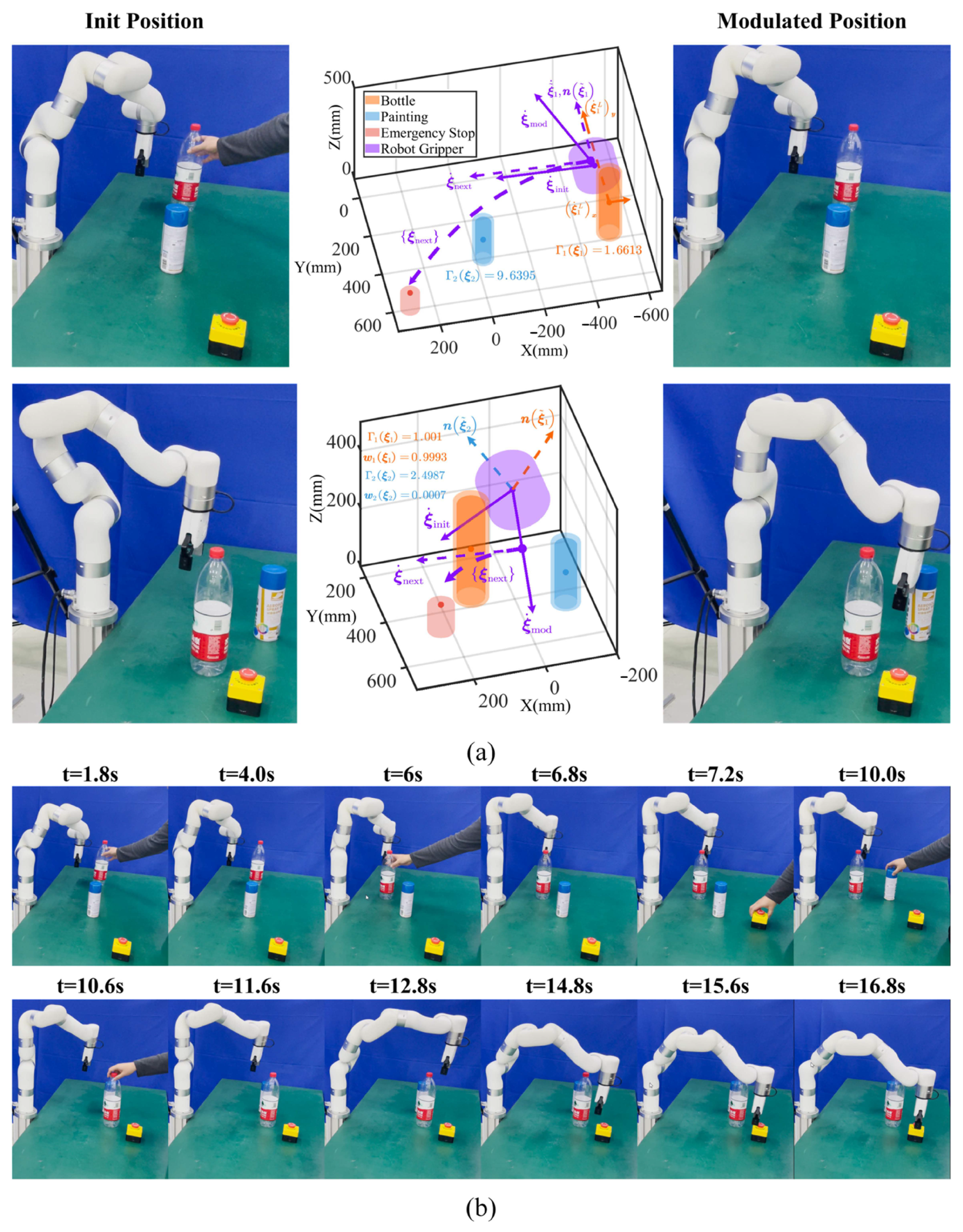
5.3. Real-Time Whole-Body Movement Adaptation

Following offline robot movement adaptation under static scenarios, we further evaluate our real-time whole-body movement adaptation method presented in Section 4 under the dynamic environment manifested as multiple stationary or moving obstacles, new target points, etc. Specifically, we first perform Algorithm 1 with the presence of a single obstacle (blue painting) and the emergency stop. The robot then randomly selects from three skills, namely, moving above, left, and right around the obstacle to generate the initial task execution trajectory. During task execution, the human gets involved in the process by suddenly moving a big bottle towards the gripper (see Figure 8b at t = 1.8 s), changing the obstacle and emergency stop positions in real-time (see Figure 8b at t = 6 s, 7.2 s, and 10.0 s, etc.).

We utilize YOLO to detect the object 3D positions and velocities at $dt$ = 0.2 s intervals with an ellipsoid-shaped distance function $\mathsf{\Gamma }\left({\mathit{\xi }}_k\right)$ enveloped (see Equation (36)). We treat the emergency stop as the target object with other objects considered obstacles. To formulate $\mathsf{\Gamma }\left({\mathit{\xi }}_k\right)$, we set the curvature parameter $p_i^k=10$ and derive the center ${\mathit{\xi }}_k^c$, linear velocities ${\dot{\mathit{\xi }}}_k^L$, and angular velocities ${\dot{\mathit{\xi }}}_k^R$ from YOLO. We obtain the normal vector $\mathit{n}\left({\tilde{\mathit{\xi }}}_k\right)$ from Equation (39) and formulate the basis matrix $\mathit{E}\left({\mathit{\xi }}_k\right)$ and the diagonal eigenvalue matrix $\mathit{D}\left({\mathit{\xi }}_k\right)$ from Equations (40) and (42). In this paper, we model the robot gripper with the same ellipsoid-function to derive equivalent $\mathsf{\Gamma }\left({\mathit{\xi }}_k\right)$ and $\mathit{n}\left({\tilde{\mathit{\xi }}}_k\right)$ from two ellipsoids. We set a 10 mm margin for each direction to compute the corresponding safety magnitude ${\eta }_k$, define the reactivity parameter ${\rho }_k=1$, and remedy the tail-effect via $\mathit{n}{\left({\tilde{\mathit{\xi }}}_k/{\eta }_k\right)}^T{\dot{\mathit{\xi }}}_k$ to formulate Equation (43). Meanwhile, we disregard the impact of obstacles when $\mathsf{\Gamma }\left({\mathit{\xi }}_k\right)>4.0$. Given the initial task execution trajectory as input, the robot performs whole-body adaptation for real-time modulation (see Figure 4). Concerning end-effector adaptation, we derive the modulation matrix $\mathit{M}\left({\mathit{\xi }}_k\right)\in {\mathbb{R}}^{3\times 3}$ and weight coefficient ${\mathit{w}}_k\left({\mathit{\xi }}_k\right)$ for each dynamic obstacle with weighted magnitude ${\parallel \mathit{Q}\left(\tilde{\mathit{\xi }}\right)\parallel }_{\mathrm{all}}$ and directions $\mathit{q}{\left(\tilde{\mathit{\xi }}\right)}_{\mathrm{all}}$ computed from Equations (46)–(52) to derive the modulted velocity ${\dot{\mathit{\xi }}}_{\mathrm{mod}}$. Regarding the non-end-effector adaptation, we detect the closest point $C_0$ with ${\mathit{x}}_{\mathit{v}}^0$ defined to perform null-space velocity control (see Section 4.2).

We conduct 10 dynamic experiments for each of the three skills by randomly placing and changing the objects, including obstacles and emergency stop, in real-time to evaluate the robot movement adaptation competence; the results are shown in Figure 8. Considering space restrictions, we select typical modulation cases for specific timesteps, as shown in Figure 8a, and choose one episode of moving above around the obstacle with snapshots, as shown in Figure 8b.

During the above experiments, considering the detected minimum distance $\parallel {\mathit{d}}_0\parallel$ for the robot, link1 to link6 are always larger than the safety margin ${\mathit{d}}_m$ = 10 mm (see Figure 3), null-space velocity control for the robot non-end-effector is not required, and we only denote end-effector modulation, as shown in Figure 8a. The left, middle, and right columns denote the robot init positions, modulation process, and modulated positions, respectively.

In the first row, the human suddenly moves a big bottle towards the robot end-effector with relative X and Y linear velocities ${\left({\dot{\mathit{\xi }}}_1^L\right)}_{\mathit{x}}=2.22\mathrm{mm}/\mathrm{s},{\left({\dot{\mathit{\xi }}}_1^L\right)}_{\mathrm{y}}=117.13\mathrm{mm}/\mathrm{s}$, the distance functions for the big bottle ${\mathsf{\Gamma }}_1\left({\mathit{\xi }}_1\right)=1.6613$ and blue painting ${\mathsf{\Gamma }}_2\left({\mathit{\xi }}_2\right)=9.6395$ are derived. As ${\mathsf{\Gamma }}_2\left({\mathit{\xi }}_2\right)=9.6395>4$, we ignore the influence of the blue painting, and the robot only modulates in response to the big bottle. We define the weight term ${\mathit{w}}_1^{\mathrm{rel}}$ to smooth the distance influence and obtain the weighted relative velocity ${\dot{\tilde{\mathit{\xi }}}}_{\mathrm{all}}$ from Equation (45); the direction coincides with the normal vector $\mathit{n}\left({\tilde{\mathit{\xi }}}_1\right)$. Given the init velocity ${\dot{\mathit{\xi }}}_{\mathrm{init}}$, we compute the diagonal eigenvalue matrix $\mathit{D}\left({\mathit{\xi }}_1\right)$ and the basis matrix $\mathit{E}\left({\mathit{\xi }}_1\right)$ to formulate the modulation matrix $\mathit{M}\left({\mathit{\xi }}_1\right)$. The modulated velocity ${\dot{\mathit{\xi }}}_{\mathrm{mod}}$ is then computed from Equation (46) with one single obstacle. We apply velocity integration to obtain the expected position for the next timestep, generalize new trajectory sets $\left\{{\mathit{\xi }}_{\mathrm{next}}\right\}$ (see Section 2.1) at the current position, and compute the next velocity ${\dot{\mathit{\xi }}}_{\mathrm{next}}$ with position differencing, treating this as the initial velocity for subsequent modulation. After modulation, we discover that there is an evident backward movement for the robot in the right column.

In the second row, the init robot position after the last timestep modulation will collide with the big bottle, and the robot is subject to the combined effects of multiple obstacles. Distinct from [31], in this paper, if the robot init position will collide, we develop the method by iteratively modulating positions until they are collision-free. Specifically, to ensure the impenetrability of obstacles, we set the big bottle and blue painting distance function ${\mathsf{\Gamma }}_1\left({\mathit{\xi }}_1\right)=1.001,{\mathsf{\Gamma }}_2\left({\mathit{\xi }}_2\right)=2.4987$ with the distance weights derived from Equation (44) as ${\mathit{w}}_1\left({\mathit{\xi }}_1\right)=0.9993,{\mathit{w}}_2\left({\mathit{\xi }}_2\right)=0.0007$. Given the normal vector $\mathit{n}\left({\tilde{\mathit{\xi }}}_1\right),\mathit{n}\left({\tilde{\mathit{\xi }}}_2\right)$, we iteratively compute the modulation matrix $\mathit{M}\left({\mathit{\xi }}_1\right),\mathit{M}\left({\mathit{\xi }}_2\right)$ for each obstacle and derive the weighted magnitude ${\parallel \mathit{Q}\left(\tilde{\mathit{\xi }}\right)\parallel }_{\mathrm{all}}$ and direction $\mathit{q}{\left(\tilde{\mathit{\xi }}\right)}_{\mathrm{all}}$ from Equations (47)–(52) to obtain the modulated velocity ${\dot{\mathit{\xi }}}_{\mathrm{mod}}$ until safe. New trajectory sets $\left\{{\mathit{\xi }}_{\mathrm{next}}\right\}$ are generalized and the next velocity ${\dot{\mathit{\xi }}}_{\mathrm{next}}$ is computed. Note that if the emergency stop position changes, the robot can adapt in real-time with our trajectory generalization method. Figure 8b shows robot dynamic modulation snapshots with multiple dynamic obstacles and changing targets (the emergency stop). The total running time is 16.8 s with 84 timesteps, and the average modulation time for a single timestep is 0.1356 s. The results indicate that the robot exhibits real-time adaptation proficiency under dynamic environments.

For the above end-effector modulation experiments, considering the minimum distances between the robot non-end-effector and obstacles are always larger than the safety margin ${\mathit{d}}_m=10\mathrm{mm}$, the non-end-effector adaptation proposed in Section 4.2 is not involved. Consequently, to further verify the mutual performance of end-effector and non-end-effector adaptation, we elevate the obstacle height and design a task scenario where the robot non-end-effector will collide with the big bottle at the beginning of task execution (see the first row of Figure 9a), and after the robot moves around, the human places the big bottle to a new position where the robot non-end-effector will collide when it tends to grasp the emergency stop (see the last row of Figure 9a).

The robot selects the move above skill to generate the initial task trajectory; the typical modulation process is shown in Figure 9a with task execution snapshots shown in Figure 9b. The left, middle, and right columns in Figure 9a denote the initial joint configurations, the modulation process, and the modulated joint configurations, respectively. To achieve real-time efficiency, we utilize cylinders to envelop obstacles and robot links with minimum distance detected by the Flexible Collision Library (FCL). To balance offline-optimized Joint ProMPs and null-velocity contol, we set $\lambda =1,\gamma =0.2,\rho =0.8$ to formulate Equation (65), and we set ${\mathit{d}}_m=10,{\mathit{d}}_n=5,v_n=10\mathrm{mm}/\mathrm{s}$ to formulate Equation (66).

The first row illustrates the robot whole-body modulation at the beginning. Given the distance function ${\mathsf{\Gamma }}_1\left({\mathit{\xi }}_1\right)=1.7806,{\mathsf{\Gamma }}_2\left({\mathit{\xi }}_2\right)=8.9839>4$, the robot is modulated under the big bottle normal vector $\mathit{n}\left({\tilde{\mathit{\xi }}}_1\right)$ with the expected end-effector modulated velocity ${\dot{\mathit{\xi }}}_{\mathrm{mod}}$. We detect the collision at the current position. To ensure impenetrability of the obstacles, we set $\parallel {\mathit{d}}_0\parallel =0.01\mathrm{mm}$ and iteratively apply null-space velocity control until safe. To be specific, we treat the robot collision link center as the control point $C_0$ and derive the Jacobian matrix ${\mathit{J}}_0$ at $C_0$. We compute the retreat velocity $v_0$ from Equation (66) and obtain the enforced velocity ${\mathit{x}}_{\mathit{v}}^0$. We then utilize the control loop defined in Equation (69) to derive the modulated joint configuration ${\mathit{q}}_{\mathrm{mod}}$ iteratively. Note that if the modulated joint configurations will collide, we increase the magnitude order of $v_0$ until safe. The middle column shows the initial and modulated joint configurations colored in purple and green, and the right column demonstrates that the robot non-end-effector heads away from the big bottle while keeping the expected end-effector positions.

The second row shows the robot end-effector modulation with the big bottle and blue painting ${\mathsf{\Gamma }}_1\left({\mathit{\xi }}_1\right)=2.5283,{\mathsf{\Gamma }}_2\left({\mathit{\xi }}_2\right)=2.7075$; the robot non-end-effector will collide at this position with $\parallel {\mathit{d}}_0\parallel =0.01\mathrm{mm}$. We define the enforced velocity ${\mathit{x}}_{\mathit{v}}^0$ to obtain the modulated joint configurations iteratively until safe, and the robot tends to move away from the big bottle when approaching the emergency stop to grasp. Figure 9b illustrates robot task execution snapshots; the total running time is 13.8 s with 69 timesteps, and the average modulation time for a single timestep is 0.1757 s. The results demonstrate that our method can simultaneously perform end-effector and non-end-effector modulation in real-time, allowing the robot to adapt joint configurations in confined spaces while keeping its expected end-effector poses.

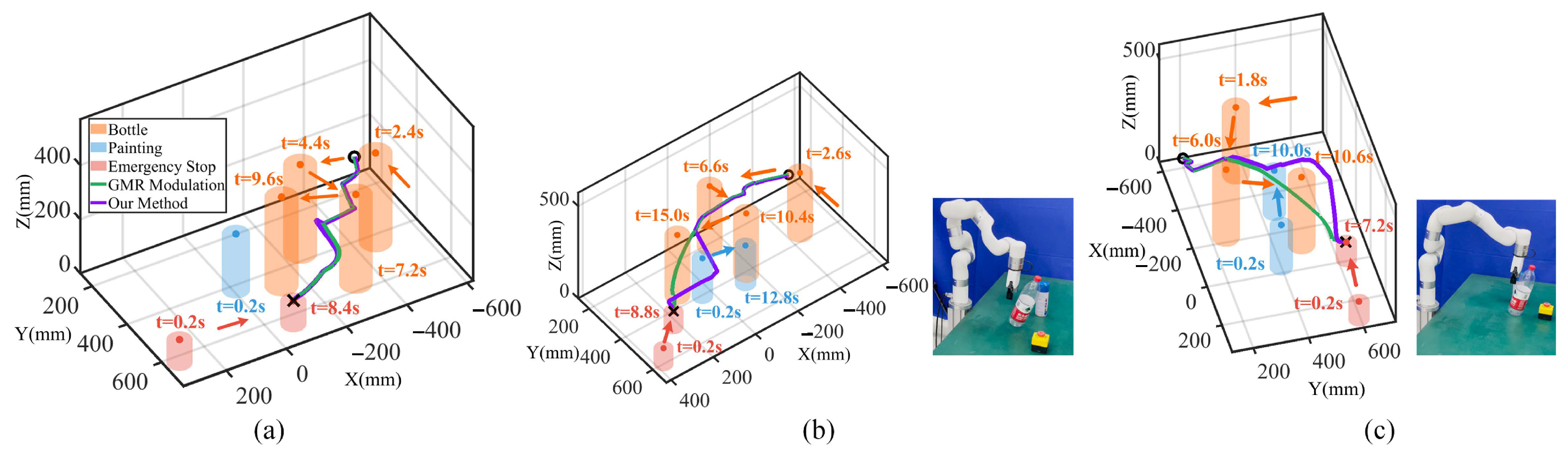
5.4. Comparative Experiments

In this paper, we propose a combined strategy for robot offline and real-time movement adaptation based on human–robot skill transfer. To validate the performance, we conduct several comparative experiments for proposed methods in the strategy.

5.4.1. Offline Movement Adaptation

Concerning offline movement adaptation, KMPs were proposed to address the limitation of explicitly defining the basis functions in ProMPs. The KMPs method was first introduced in [11] by employing GMM/GMR to encode the demonstrated distribution and then deriving the mean and covariance of each timestep under via-points based on dual transformation and KL divergence. The most notable contribution was the derivation of a kernel matrix that depends only on each timestep, eliminating the need to explicitly define the basis functions and reducing the dimensionality of the parameters. Furthermore, they extended KMPs to incorporate linear constraints in [22] (LC-KMPs), allowing for the rapid acquisition of optimal Lagrange multipliers via quadratic programming (QP). However, this method can only be applied to linear constraints in Cartesian space. In [23], they further extended LC-KMPs to incorporate nonlinear constraints (EKMPs) by using Taylor expansion to convert the problem into a QP problem and solve the optimal Lagrange multipliers. This approach can handle various nonlinear constraints in Joint space. To account for all task constraints, especially including collisions between the robot’s other links and obstacles, optimization needs to be performed in Joint space. As a result, to further compare the performance, we select EKMPs from [23] and the ProMPs-based method from [21], which is similar to ours.

We take the danger scene (see Figure 7a) with the same task constraints to compare. For the three methods, we provide the same initial collision-free trajectory sets of the robot end-effector and obtain the corresponding Joint space distributions with Jacobian IK. Some joint distributions may lead to collisions between the robot links 1 to 6 and obstacles. The goal is to optimize these distributions to generate new joint configurations for task execution. We then execute the task 100 times and evaluate the methods based on several metrics as follows: number of optimization parameters, number of constraints, total iterations, optimization time, distribution loss, and task success rate. The results are shown in

Table 2. Robot offline movement adaptation comparison. We set the same task constraints in the danger scene (Figure 7a). Given the initial collision-free end-effector trajectory sets, we obtain the corresponding Joint space distributions using Jacobian IK. Some Joint distributions may lead to collisions for robot links 1 to 6, and the goal is to optimize the distributions for task execution, which is then performed 100 times.

	Algorithm in [21]	EKMPs in [23]	Our Method
Parameters for Optimization	665	512	777
Constraints Formulas $F_{c_{k,t}}$ Numbers	512	512	136
Total Iteration Numbers	265	36	64
Optimization Time (s)	853.36	728.58	126.45
Distribution Loss	76.48%	70.32%	84.36%
Task Success Rate	92%	91%	99%

.

In [21], the number of optimization parameters mainly includes the weights and covariance matrices of the 35 basis functions in ProMPs. Due to the use of Cholesky decomposition, a total of $35+18\times 35=665$ parameters needs optimization. For 30 timesteps, each timestep involves 7 joint range constraints, 4 hyperplane constraints, 6 repellers constraints (from robot links 1 to 6), and waypoints constraints for the start and end points, resulting in a total of $(7+4+6)\times 30+2=512$ constraints.

In EKMPs [23], the optimization targets the Lagrange multipliers that define the task constraints, with a quadratic programming (QP) approach employed. As a result, the number of optimization variables is equal to the number of task constraints, which is 512. Using the optimal multipliers, a kernel matrix is constructed to derive the mean and covariance for each timestep.

In our method, before optimization, the overall ProMP distributions are decoupled into the mean and standard deviation for each timestep. We then identify timesteps that may violate the task constraints based on the mean and standard deviation at each timestep. We find that there are 8 timesteps violating the task constraints, and the waypoint constraints at the start and end points are already satisfied, resulting in $(7+4+6)\times 8=136$ constraints. In addition to optimizing the mean and covariance of ProMPs, we also optimize the mean and standard deviation of the joint positions for the 8 timesteps with $665+14\times 8=777$ parameters in total.

During optimization, we discover that the algorithm in [21] integrates all nonlinear task constraints with $\left({\mathit{\mu }}_{\mathit{w}},{\mathbf{\Sigma }}_{\mathit{w}}\right)$ for each timestep. This integration necessitates the evaluation of symmetric positive definiteness for the covariance matrix ${\mathbf{\Sigma }}_{\mathit{w}}$ during optimization, resulting in the most iterations and the longest optimization time. EKMPs [23], which involve large matrix computations, also encounter numerical instability. Specifically, as the number of timesteps and task constraints increases, the matrix size grows, and many matrix parameters become unstable during inversion. Some elements may also become redundant, which is a characteristic of the KMP formulation. Although QP optimization reduces the number of iterations, the extensive matrix computations required to calculate the mean and covariance at each timestep still lead to longer optimization times.

In contrast, our method essentially decouples the ProMP parameters to each timestep and identifies the feature timesteps that violate task constraints, optimizing the distribution for those specific timesteps separately. Notably, after optimizing the mean and standard deviation, the optimization of the mean and covariance of ProMPs becomes linear in terms of ${\mathit{\mu }}_{\mathit{w}}$ and ${\mathbf{\Sigma }}_{\mathit{w}}$, which avoids introducing numerical instability. Here, we do not rely on ProMPs’ inherent ability to generate new parameters. Instead, we address the issue of ProMPs’ limited extrapolation ability through optimization. However, since our method utilizes TensorFlow’s automatic differentiation rather than a QP formulation, the total number of iterations is slightly higher than that of EKMP. Nonetheless, the optimization time in our method is significantly reduced due to improved numerical stability.

Furthermore, we evaluate the generalization capability of each algorithm. In this context, generalization refers to the ability to maintain the initial distribution when encountering different task constraints and to achieve a high success rate. Specifically, if the optimized distribution closely matches the original distribution and achieves a high success rate, the method is considered to have strong generalization. The results show that [21] retains more of the original distribution compared to EKMPs [23]. However, in [21], due to the use of the unscented transform, which is sensitive to the coefficients, the estimates for ${\mathit{\mu }}_{\mathit{w}}$ and ${\mathbf{\Sigma }}_{\mathit{w}}$ under task constraints are inaccurate. This leads to unfiltered joint distributions that violate the task constraints, resulting in task failures. Similarly, EKMP’s use of Taylor linear expansion does not separate out some failed distributions, leading to a lower task success rate.

Our method, however, after obtaining the optimized joint distributions, introduces a threshold to mitigate the distribution loss caused by the probabilistic characteristics. Specifically, the robot first generates task trajectories with via-point generalization, obtains the corresponding inverse kinematics solutions, and then evaluates the number of solutions within the optimized joint range. If this number exceeds the threshold, the robot executes the task. This approach reduces the distribution loss and improves success rates. The threshold determination process is obtained by sampling the via-points and recording the task execution results and the number of inverse solutions. However, due to the discrete nature of via-points, when the threshold intersects with continuous space, the optimization algorithm indicates task success, but the robot can fail. This issue requires more continuous via-point ranges for accurate task execution.

Overall, despite the higher number of optimization parameters, our method achieves reduced optimization time and higher success rates by decoupling the mean and Gaussian distribution for each timestep and employing a dual optimization process for the ProMP parameters. These results demonstrate the high generalization capability of our method. Our method exhibits efficiency at the cost of increasing optimization parameters. The optimization time cannot fulfill real-time needs; however, the robot is equipped with flexible skills incrementally augmented from human demonstrations before online task execution.

5.4.2. Real-Time Movement Adaptation

Concerning robot real-time movement adaptation based on imitation learning (IL), ref. [47] first proposes the method of learning stable nonlinear dynamical systems (SEDS) with GMM-GMR. They utilize GMM to learn the relation of the Cartesian positions and velocities. Given the current positions, they use GMR to generate the velocities for task execution. They further develop the method in [30,31], and ref. [32] to achieve real-time movement adaptation for the robot end-effector. In this paper, we compare our method to theirs (SEDS-GMR modulation) under the same dynamic environment (see Figure 8b). To be specific, the robot randomly generates the initial task execution trajectory from three skills (moving above, left, and right around obstacles). During task execution, the human gets involved by placing and changing objects in real-time. Given the initial task execution trajectories, we choose 6 Gaussian kernels and train the optimal GMM parameters with 1000 iterations offline to ensure accurate trajectory reproduction via GMR. We conduct 10 experiments for each skill with the qualitative and quantitative results shown in Figure 10 and

Table 3. Robot end-effector modulation comparision.

	SEDS-GMR Modulation [30,31]	Our Method
Task Success Rate	73.33%	93.33%
Offline Parameters Learning Time (s)	24.6856 ± 0.1546	0.0904 ± 0.0148
Average Real-time Modulation Time (s)	0.1238 ± 0.0167	0.1465 ± 0.0285
Total Task Execution Time (s)	23.2 ± 1	16.8 ± 0.4
Collison Rate	26.67%	6.67%
Final Position Error (mm)	0.52 ± 0.13	0.55 ± 0.09
Convergence TimeSteps	116 ± 5	84 ± 2

. Figure 10a denotes 3D positions modulation when the robot selects to move right around the obstacle. We discover that the modulation remains consistent for both methods if the init 3D positions before modulation will not collide with the obstacle. However, if the collision occurs for the init positions (see Figure 10b,c), SEDS-GMR modulation will not ensure the process is collision-free despite the modulation matrix influence.

In contrast, our method iteratively performs modulation until collision-free; that is, if the modulated positions will collide, we treat them as init positions and modulate them until safe. Note that our method may fail in specific danger cases: if the robot iterates many times for modulation, during the motion process from the current position to the modulated position, collision will occur. However, in most cases, our method ensures a high success rate.

Table 3 shows several benchmarks for both methods. Our method exhibits a higher success rate. In addition, since SEDS-GMR modulation requires obtaining precise GMM parameters before task execution, the offline training time is longer. Our method generalizes the trajectories in real-time without training parameters (see Section 2.1) and computes the velocities via position differencing. Although our method involves iterating the modulation when encountering collisions, resulting in a relatively longer time for single-step modulation, it still meets real-time requirements. Moreover, our method outperfoms SEDS-GMR modulation in total task execution time, requiring fewer convergence timesteps and exhibiting a lower collision rate. The final position error effectively reflects the accuracy of the modulation in achieving the desired end-effector position while ensuring obstacle avoidance. Both methods achieve comparable final position accuracy, confirming that our approach maintains accuracy while ensuring obstacle avoidance. The results indicate that our method can complete real-time end-effector modulation while ensuring safety, and quickly generalize trajectories preserving human skill characteristics.

The aforementioned comparison experiments with SEDS-GMR only consider the robot end-effector given that the other robot links will not collide during task execution. To further evaluate the robot whole-body movement adaptation performance, we conduct comparison experiments under the scene in Figure 9. We select a commonly-used trajectory planner named Covariant Hamiltonian Optimization for Motion Planning (CHOMP) which iteratively optimizes the cost function including trajectory smoothness and collision cost; meanwhile, a null space velocity control method [36] similar to ours is involved.

As in Figure 9, we obtain the modulated robot end-effector trajectory with 69 timesteps. For all methods, we set the same expected 3D positions at each timestep and test the robot non-end-effector modulation performance. We repeat 30 experiments with the results shown in Figure 11 and

Table 4. Robot non-end-effector modulation comparision.

	CHOMP	Null Space Control in [36]	Our Method
Success Rate	93.33%	76.67%	96.67%
Average Modulation Time (s)	0.1434 ± 0.0563	0.1654 ± 0.0146	0.1757 ± 0.0086
Joint Configurations Iterations	126 ± 24	10 ± 2	20 ± 1
Modulation Path (m)	9.8829 ± 1.2368	0.8204 ± 0.0046	0.8232 ± 0.0024
Total Task Execution Time (s)	232.8 $\pm 60.2$	13.2 $\pm 0.6$	13.8 ± 0.4
Collision Rate	6.67%	23.33%	3.33%
Final Position Error (mm)	0.83 ± 0.16	0.66 ± 0.14	0.59 ± 0.06

. The first row of Figure 11 shows that CHOMP may occasionally generate erratic and random joint configurations when collisions are detected. Additionally, unnecessary spaces are utilized to reach the desired positions, leading to redundant planning. The null space control method in the second row employs a fixed retreat velocity ${\mathit{x}}_{\mathit{v}}^0$, leading to collisions when the velocity is insufficient to maneuver the robot non-end-effector away from the obstacles. In contrast, our method iteratively employs null space velocity control, gradually increasing ${\mathit{x}}_{\mathit{v}}^0$ until collison-free to ensure safety, as shown in the last row.

Quantitative results are presented in Table 4. For each experiment, we compute the average single-step modulation time and the total joint configuration iterations, namely, the intermediate joint configurations traversed to the expected 3D positions. Additionally, the Cartesian modulation path lengths for the end-effector are derived. We discover that CHOMP achieves a 93.33% success rate with a shorter average single-step modulation time. However, due to its stochastic nature, it generates a large number of random trajectories, leading to significantly longer modulation paths and higher variability. As a result, the total task execution time is longer. The null space control method yields a lower success rate, as the enforced velocity could not ensure collision-free joint configurations. However, since it only performs a single iteration, the overall execution time is relatively short. Compared to these methods, our approach iterates multiple times to ensure joint configuration safety. While this results in a slightly longer overall execution time, it remains within a reasonable range and meets real-time requirements. Additionally, our method exhibits a lower collision rate, as the iterative process effectively prevents unsafe configurations. The final position error reflects the precision of our approach in maintaining accuracy while successfully completing the obstacle avoidance task. The results indicate that our method enables real-time robot whole-body movement adaptation with a high success rate. When potential collisions for the robot non-end-effector occur, our method can obtain joint configurations through iterations in real-time with minor deviations for the modulated path. By integrating offline optimization and online dynamic modulation, our method can adapt to different robotic tasks by incrementally augmenting skills from human demonstrations offline and performing real-time movement adaptation during task execution.

6. Discussion

6.1. Comparison to Previous Work

This paper proposes a human–robot skill transfer strategy including basic-level MPs learning, core-level MPs adaptation, and real-time robot whole-body adaptation. Considering basic-level MPs learning, we develop the via-point trajectory generalization method adapting to the task start, end, and via-points from only one human demonstration. Our approach ensures robust extrapolation beyond the demonstration range. By discretizing the via-points, we can efficiently generate a large set of trajectory sets without additional demonstrations. These skills are encoded using ProMPs, preserving the probabilistic properties. In other words, the proposed via-point generalization enhances the extrapolation capability of ProMPs [10], while retaining key probabilistic characteristics, like the mean and covariance.

Considering core-level MPs adaptation, we develop an effective task-constrained optimization method by combining multiple task constraints into a unified probabilistic framework. To account for all task constraints in Joint and Cartesian space simultaneously, we encode ProMPs in Joint space. We introduce a double-loop optimization method with ProMPs, where each timestep is first decoupled as the Gaussian distribution, and only those timesteps violating task constraints are optimized. After optimizing the Gaussians at each timestep, a second optimization is performed to obtain the optimized ProMPs. To mitigate the loss of distributions due to the probabilistic nature, we introduce a threshold to directly utilize the ProMPs for task execution with analytical movement adaptation.

To evaluate MPs adaptation performance under different task constraints, three performance indices are considered as follows: (i) Computational Efficiency denotes the number of parameters, iterations, and runtime required to derive the optimized MPs; (ii) Constraint Diversity Satisfaction refers to whether MPs can simultaneously handle multiple types of task constraints in both Joint and Cartesian space; and (iii) Generalization Capability evaluates whether the optimized MPs can retain the distribution of original MPs while successfully executing tasks across different task scenarios. Our method ensures the Constraint Diversity Satisfaction to handle multiple task constraints in Joint and Cartesian space. Compared to [21], our method avoids symmetric positive-definite issues during iterations by decoupling the Gaussians for each timestep and optimizing the ProMPs independently. Furthermore, unlike EKMPs [23], our method does not involve large matrix computations or numerical stability issues, resulting in improved Computational Efficiency. Additionally, we estimate nonlinear task constraints with different probability distributions, rather than first-order Taylor expansions, thus exhibiting robust generalization capabilities compared to EKMPs [23]. By incorporating a threshold that accounts for the probabilistic nature, our method exhibits robust generalization compared to [21].

Considering real-time movement adaptation, we propose an improved real-time robot whole-body control method integrating offline task-constrained optimization. For the robot end-effector, we incorporate the offline-optimized trajectory with via-point generalization for dynamic modulation, and develop DSM by performing multiple modulation iterations until safe if initial positions will collide, while satisfying real-time needs. For the robot non-end-effector, we integrate the offline-optimized Joint ProMPs to the real-time null space velocity control method and ensure collision-free joint configurations through iterations.

6.2. Limitations and Future Work

Although the proposed strategy has made some progress, it still faces certain limitations that require further investigation. The method demonstrates strong performance in environments with a moderate number of obstacles; however, its effectiveness in extremely confined spaces remains an area needing refinement. In such scenarios, joint configurations become highly constrained, and the iterative modulation process may lead to slower convergence or even failure to identify feasible solutions. Future efforts should prioritize enhancing the iterative adjustment process in confined environments by incorporating more detailed task constraints and refining the dynamic modulation strategies. These improvements would ensure more reliable performance in such challenging settings.

Another notable limitation lies in the iteration time for real-time modulation, particularly for applications demanding ultra-fast responses on commercially available robotic systems. Although our method achieves real-time performance in most cases, further reducing iteration times to meet the requirements of ultra-fast response applications remains an unresolved challenge. Potential avenues for improvement include leveraging deep learning techniques or heuristic approaches to reduce the computational overhead, as well as fine-tuning the interpolation times and refresh rates to enhance speed.

Moreover, although our method has been validated on a specific robotic arm, its generalization across different robotic platforms with varying degrees of freedom and kinematic configurations remains to be thoroughly evaluated. Expanding testing to include diverse robotic systems would provide a more comprehensive assessment of its applicability. Additionally, comparing our approach with other state-of-the-art algorithms in human–robot skill transfer, as well as evaluating its performance in environments with increased obstacle density and stricter motion constraints, would offer deeper insights into its versatility and scalability. Finally, exploring the extension of this strategy to more complex tasks, such as the manipulation of deformable objects or operation in environments with higher uncertainty, represents a promising direction for future research.

7. Conclusions

This paper presents a strategy for human–robot skill transfer with offline task-constrained optimization and real-time whole-body modulation. The human only needs to provide one demonstration to teach the robot one skill category. Continuous ProMPs distributions can be obtained with discrete via-points from the proposed via-point trajectory generalization method. Facing task constraints under new task scenarios, the objective is to optimize ProMPs by excluding specific regions. The proposed effective probabilistic optimization method can incorporate task constraints in Joint and Cartesian space conveniently to derive optimized ProMPs. We define the threshold enabling the robot to accomplish tasks directly without checking the task constraints for each timestep. Additionally, the human can incrementally demonstrate new skills to the robot when the current skills cannot complete the task.

Once the robot selects a specific skill for task execution, in the face of multiple dynamic obstacles, we propose a real-time adaptive control method for robot whole-body obstacle avoidance. The method solves the collision problem in DSM that may occur during the convergence towards a target. We utilize modulations iteratively to obtain the expected end-effector positions in real-time with no need to stop moving, which increases the success rate. Moreover, for non-end-effector obstacle avoidance, we propose the improved null-space velocity control method independent of manually defined retreat velocities by deriving safe joint configurations through iterations, ensuring a high success rate and stable behavior with reduced randomness.

The proposed strategy makes robot task execution more flexible. In the offline phase, we can provide the robot with different skills without adhering to specific task constraints. After ProMPs optimization under new task-constrained scenarios, the robot selects randomly from the feasible skills. During task execution, the proposed real-time whole-body adaptation method can modulate in real-time under dynamic environments, which benefits human-robot coexistence in manufacturing. The proposed strategy may fail in very narrow spaces. However, in most cases, the proposed strategy can avoid obstacles in advance with the weighted influence of multiple dynamic obstacles. The experimental results demonstrate that our method can ensure a high success rate while meeting real-time requirements. The strategy is general and can be applied to other redundant robotic arms.

Concerning the potential scalability of the proposed strategy to other frameworks that do not necessarily use ProMPs, in this paper, we first generalize a large set of collision-free trajectories through via-point generalization from a single human demonstration. To denote different ways of completing the task, we can use other probabilistic frameworks to encode the distribution. We decouple ProMPs into Gaussian distributions at each timestep, optimizing Gaussians for those time steps violating task constraints, and then obtain the optimized ProMPs separately. This approach can be extended to other probabilistic methods, such as using the GMM to model the overall Gaussian distributions and obtain the mean and standard deviation for each timestep with GMR. By applying our task-constrained optimization methods, the Gaussian distributions for each timestep can be optimized with new probability distributions derived by the characteristics of other probabilistic methods. For real-time movement adaptation, we integrate the optimized trajectory for end-effector dynamic modulation. This process can also be used with other MPs to generalize real-time trajectories. Meanwhile, we incorporate Joint ProMPs into the null space velocity control formulation. For other probabilistic methods, the formulation will integrate their probabilistic nature so that during real-time movement adaptation, the robot can preserve the offline-optimized distributions.

Future work will focus on enabling robotic arms to perform more complex tasks in extremely confined spaces, such as opening doors or manipulation of deformable objects, while avoiding obstacles in real-time.

References

1. Mukherjee, D.; Gupta, K.; Chang, L.H.; Najjaran, H. A survey of robot learning strategies for human-robot collaboration in industrial settings. Robot. Comput.-Integr. Manuf. 2022, 73, 102231. [Google Scholar] [CrossRef]
2. Argall, B.D.; Chernova, S.; Veloso, M.; Browning, B. A survey of robot learning from demonstration. Robot. Auton. Syst. 2009, 57, 469–483. [Google Scholar] [CrossRef]
3. Zhu, Z.; Hu, H. Robot learning from demonstration in robotic assembly: A survey. Robotics 2018, 7, 17. [Google Scholar] [CrossRef]
4. Calinon, S. Learning from demonstration (programming by demonstration). Encycl. Robot. 2018, 1–8. [Google Scholar] [CrossRef]
5. Correia, A.; Alexandre, L.A. A survey of demonstration learning. Robot. Auton. Syst. 2024, 182, 104812. [Google Scholar] [CrossRef]
6. Zare, M.; Kebria, P.M.; Khosravi, A.; Nahavandi, S. A survey of imitation learning: Algorithms, recent developments, and challenges. IEEE Trans. Cybern. 2024, 54, 7173–7186. [Google Scholar] [CrossRef] [PubMed]
7. Jaquier, N.; Zhou, Y.; Starke, J.; Asfour, T. Learning to sequence and blend robot skills via differentiable optimization. IEEE Robot. Autom. Lett. 2022, 7, 8431–8438. [Google Scholar] [CrossRef]
8. Ijspeert, A.J.; Nakanishi, J.; Hoffmann, H.; Pastor, P.; Schaal, S. Dynamical movement primitives: Learning attractor models for motor behaviors. Neural Comput. 2013, 25, 328–373. [Google Scholar] [CrossRef]
9. Calinon, S.; Guenter, F.; Billard, A. On learning, representing, and generalizing a task in a humanoid robot. IEEE Trans. Syst. Man Cybern. Part B (Cybernetics) 2007, 37, 286–298. [Google Scholar] [CrossRef]
10. Paraschos, A.; Daniel, C.; Peters, J.; Neumann, G. Using probabilistic movement primitives in robotics. Auton. Robot. 2018, 42, 529–551. [Google Scholar] [CrossRef]
11. Huang, Y.; Rozo, L.; Silvério, J.; Caldwell, D.G. Kernelized movement primitives. Int. J. Robot. Res. 2019, 38, 833–852. [Google Scholar] [CrossRef]
12. Li, G.; Jin, Z.; Volpp, M.; Otto, F.; Lioutikov, R.; Neumann, G. ProDMP: A Unified Perspective on Dynamic and Probabilistic Movement Primitives. IEEE Robot. Autom. Lett. 2023, 8, 2325–2332. [Google Scholar] [CrossRef]
13. Lauretti, C.; Cordella, F.; Zollo, L. A hybrid joint/Cartesian DMP-based approach for obstacle avoidance of anthropomorphic assistive robots. Int. J. Soc. Robot. 2019, 11, 783–796. [Google Scholar] [CrossRef]
14. Pairet, È.; Ardón, P.; Mistry, M.; Petillot, Y. Learning generalizable coupling terms for obstacle avoidance via low-dimensional geometric descriptors. IEEE Robot. Autom. Lett. 2019, 4, 3979–3986. [Google Scholar] [CrossRef]
15. Duan, A.; Camoriano, R.; Ferigo, D.; Calandriello, D.; Rosasco, L.; Pucci, D. Constrained DMPs for feasible skill learning on humanoid robots. In Proceedings of the 2018 IEEE-RAS 18th International Conference on Humanoid Robots (Humanoids), Beijing, China, 6–9 November 2018; pp. 1–6. [Google Scholar]
16. Dahlin, A.; Karayiannidis, Y. Adaptive trajectory generation under velocity constraints using dynamical movement primitives. IEEE Control Syst. Lett. 2019, 4, 438–443. [Google Scholar] [CrossRef]
17. Paraschos, A.; Lioutikov, R.; Peters, J.; Neumann, G. Probabilistic prioritization of movement primitives. IEEE Robot. Autom. Lett. 2017, 2, 2294–2301. [Google Scholar] [CrossRef]
18. Koert, D.; Maeda, G.; Lioutikov, R.; Neumann, G.; Peters, J. Demonstration based trajectory optimization for generalizable robot motions. In Proceedings of the 2016 IEEE-RAS 16th International Conference on Humanoid Robots (Humanoids), Cancun, Mexico, 15–17 November 2016; pp. 515–522. [Google Scholar]
19. Izadi, N.H.; Palhang, M.; Safayani, M. Layered Relative Entropy Policy Search. Knowl.-Based Syst. 2021, 223, 107025. [Google Scholar] [CrossRef]
20. Koert, D.; Pajarinen, J.; Schotschneider, A.; Trick, S.; Rothkopf, C.; Peters, J. Learning intention aware online adaptation of movement primitives. IEEE Robot. Autom. Lett. 2019, 4, 3719–3726. [Google Scholar] [CrossRef]
21. Frank, F.; Paraschos, A.; van der Smagt, P.; Cseke, B. Constrained probabilistic movement primitives for robot trajectory adaptation. IEEE Trans. Robot. 2021, 38, 2276–2294. [Google Scholar] [CrossRef]
22. Huang, Y.; Caldwell, D.G. A linearly constrained nonparametric framework for imitation learning. In Proceedings of the 2020 IEEE International Conference on Robotics and Automation (ICRA), Paris, France, 31 May–31 August 2020; pp. 4400–4406. [Google Scholar]
23. Huang, Y. Ekmp: Generalized imitation learning with adaptation, nonlinear hard constraints and obstacle avoidance. arXiv 2021, arXiv:2103.00452. [Google Scholar]
24. Karaman, S.; Frazzoli, E. Sampling-based algorithms for optimal motion planning. Int. J. Robot. Res. 2011, 30, 846–894. [Google Scholar] [CrossRef]
25. Zucker, M.; Ratliff, N.; Dragan, A.D.; Pivtoraiko, M.; Klingensmith, M.; Dellin, C.M.; Bagnell, J.A.; Srinivasa, S.S. Chomp: Covariant hamiltonian optimization for motion planning. Int. J. Robot. Res. 2013, 32, 1164–1193. [Google Scholar] [CrossRef]
26. Bhardwaj, M.; Sundaralingam, B.; Mousavian, A.; Ratliff, N.D.; Fox, D.; Ramos, F.; Boots, B. Storm: An integrated framework for fast joint-space model-predictive control for reactive manipulation. In Proceedings of the Conference on Robot Learning, PMLR, Auckland, New Zealand, 14–18 December 2022; pp. 750–759. [Google Scholar]
27. Cai, M.; Aasi, E.; Belta, C.; Vasile, C.I. Overcoming exploration: Deep reinforcement learning for continuous control in cluttered environments from temporal logic specifications. IEEE Robot. Autom. Lett. 2023, 8, 2158–2165. [Google Scholar] [CrossRef]
28. Tulbure, A.; Khatib, O. Closing the loop: Real-time perception and control for robust collision avoidance with occluded obstacles. In Proceedings of the 2020 IEEE/RSJ International Conference on Intelligent Robots and Systems (IROS), Las Vegas, NV, USA, 25–29 October 2020; pp. 5700–5707. [Google Scholar]
29. Szulczyński, P.; Pazderski, D.; Kozłowski, K. Real-time obstacle avoidance using harmonic potential functions. J. Autom. Mob. Robot. Intell. Syst. 2011, 5, 59–66. [Google Scholar]
30. Khansari-Zadeh, S.M.; Billard, A. A dynamical system approach to realtime obstacle avoidance. Auton. Robot. 2012, 32, 433–454. [Google Scholar] [CrossRef]
31. Huber, L.; Billard, A.; Slotine, J.J. Avoidance of convex and concave obstacles with convergence ensured through contraction. IEEE Robot. Autom. Lett. 2019, 4, 1462–1469. [Google Scholar] [CrossRef]
32. Huber, L.; Slotine, J.J.; Billard, A. Fast obstacle avoidance based on real-time sensing. IEEE Robot. Autom. Lett. 2022, 8, 1375–1382. [Google Scholar] [CrossRef]
33. Huber, L.; Slotine, J.J.; Billard, A. Avoidance of Concave Obstacles through Rotation of Nonlinear Dynamics. IEEE Trans. Robot. 2023, 40, 1983–2002. [Google Scholar] [CrossRef]
34. Seraji, H.; Bon, B. Real-time collision avoidance for position-controlled manipulators. IEEE Trans. Robot. Autom. 1999, 15, 670–677. [Google Scholar] [CrossRef]
35. Petrič, T.; Žlajpah, L. Smooth continuous transition between tasks on a kinematic control level: Obstacle avoidance as a control problem. Robot. Auton. Syst. 2013, 61, 948–959. [Google Scholar] [CrossRef]
36. Zheng, D.; Wu, X.; Pang, J. Real-time whole-body obstacle avoidance for 7-DOF redundant manipulators. In Proceedings of the 2021 33rd Chinese Control and Decision Conference (CCDC), Kunming, China, 22–24 May 2021; pp. 2626–2631. [Google Scholar]
37. Oikonomidis, I.; Kyriazis, N.; Argyros, A.A. Efficient model-based 3D tracking of hand articulations using Kinect. In Proceedings of the British Machine Vision Conference, Dundee, UK, 29 August–2 September 2011; Volume 1, p. 3. [Google Scholar]
38. Carpentier, J.; Mansard, N. Analytical derivatives of rigid body dynamics algorithms. In Proceedings of the Robotics: Science and Systems (RSS 2018), Pittsburgh, PA, USA, 26–30 June 2018. [Google Scholar]
39. McDonald, G.C. Ridge regression. Wiley Interdiscip. Rev. Comput. Stat. 2009, 1, 93–100. [Google Scholar] [CrossRef]
40. Wan, E.A.; Van Der Merwe, R. The unscented Kalman filter for nonlinear estimation. In Proceedings of the IEEE 2000 Adaptive Systems for Signal Processing, Communications, and Control Symposium (Cat. No. 00EX373), Lake Louise, AB, Canada, 4 October 2000; pp. 153–158. [Google Scholar]
41. Bertsekas, D.P. Nonlinear programming. J. Oper. Res. Soc. 1997, 48, 334. [Google Scholar] [CrossRef]
42. Berahas, A.S.; Takáč, M. A robust multi-batch L-BFGS method for machine learning. Optim. Methods Softw. 2020, 35, 191–219. [Google Scholar] [CrossRef]
43. Abadi, M.; Agarwal, A.; Barham, P.; Brevdo, E.; Chen, Z.; Citro, C.; Corrado, G.S.; Davis, A.; Dean, J.; Devin, M.; et al. Tensorflow: Large-scale machine learning on heterogeneous distributed systems. arXiv 2016, arXiv:1603.04467. [Google Scholar]
44. Kronander, K.; Khansari, M.; Billard, A. Incremental motion learning with locally modulated dynamical systems. Robot. Auton. Syst. 2015, 70, 52–62. [Google Scholar] [CrossRef]
45. Barata, J.C.A.; Hussein, M.S. The Moore–Penrose pseudoinverse: A tutorial review of the theory. Braz. J. Phys. 2012, 42, 146–165. [Google Scholar] [CrossRef]
46. Adarsh, P.; Rathi, P.; Kumar, M. YOLO v3-Tiny: Object Detection and Recognition using one stage improved model. In Proceedings of the 2020 6th International Conference on Advanced Computing and Communication Systems (ICACCS), Coimbatore, India, 6–7 March 2020; pp. 687–694. [Google Scholar]
47. Khansari-Zadeh, S.M.; Billard, A. Learning stable nonlinear dynamical systems with gaussian mixture models. IEEE Trans. Robot. 2011, 27, 943–957. [Google Scholar] [CrossRef]
Figure 1. The proposed via-point trajectory generalization schematic. (a) 3D via-point generalization with obstacles. p and p new represent x, y, and z values over T time steps, with one via-point shown as an example. The blue cylinder denotes the obstacle, and the new via-point can be selected from above, left, or right of the obstacle for safe avoidance. (b) Orientation generalization using SLERP. At new orientations o 1 new and o 1 end , the orientation is generalized based on the quaternion multiplication of h o new and f o 1 , f o end .
Applsci 15 03171 g001
Figure 2. Dynamic system modulation for robot end-effector.
Applsci 15 03171 g002
Figure 3. Null-space velocity control for robot non-end-effector.
Applsci 15 03171 g003
Figure 4. The integrated offline and real-time robot movement adaptation control diagram.
Applsci 15 03171 g004
Figure 5. Template trajectory generalization from only one human demonstration. (a) Snapshots of human hand centroid tracking with the Kinect FORTH system. The first, middle, and last rows denote move above, left, and right around the obstacle, respectively. (b) The generalized template trajectory for three modes at the minimum Z-position of the robot gripper center with the same start point (symbol ‘o’) and end point (symbol ‘x’).
Applsci 15 03171 g005
Figure 6. Offline movment adaptation experiment with a new big bottle. (a) Experimental setup. (b) End-effector collision-free trajectory sets for three skills with via-point trajectory generalization. (c) Joint ProMPs distributions given discrete collision-free joint sets (taking the move above skill as an example). Solid lines denote mean values with shaded areas denoting ± 2 standard deviations. (d) Robot task execution snapshots: the first, middle, and last rows denote move above, left, and right around the obstacle.
Applsci 15 03171 g006
Figure 7. Offline movement adaptation experiment under a danger scene with the elevated obstacle. (a) Experimental setup. (b) Evident collision for other robot links when generalizing collision-free end-effector trajectory with certain via-points. (c) Optimized ProMPs distributions under nonlinear task constraints with LBFGS and EMM. We choose typical joint 2 and 4 distributions with obvious changes, the line and shaded areas denote the original and optimized mean and standard deviations. (d) Threshold determination based on the relationship between via-point Z-position and obstacle avoidance result. The succeed number threshold is denoted with a blue solid circle. Blue and red areas denote success and failure results. (e) Generalized task execution trajectory sets with 100 discrete via-points; red and blue lines and areas denote success and failure results. (f) Robot task execution snapshots with the critical trajectory between success and failure. The first row and last rows show different motion views.
Applsci 15 03171 g007
Figure 8. Robot end-effector real-time movement adaptation experiments. (a) Typical modulation cases for specific timesteps. The left, middle, and right columns denote the robot init positions, modulation process, and modulated positions. We utilize ellipsoids to envelop the task objects and robot gripper. (b) One episode execution snapshots when the robot selects the skill of moving above around the obstacle with 0.2 s intervals for each adjacement timestep.
Applsci 15 03171 g008
Figure 9. Robot whole-body online movement adaptation experiments. (a) Typical modulation cases for specific timesteps. The left, middle, and right columns denote the robot init joint configurations, modulation process, and modulated joint configurations. We utilize cylinders to envelop the task objects and robot links; the initial and modulated joints are colored in purple and green, respectively. (b) Task execution snapshots when the robot selects the skill of moving above around the obstacle with 0.2 s intervals for each adjacement timestep.
Applsci 15 03171 g009
Figure 10. Robot end-effector modulation comparison between SEDS-GMR and our method. Green and purple lines denote SEDS-GMR and our method, respectively. (a) Modulated 3D trajectories when the robot moves right. Arrows illustrate obstacle motion trends with cylinders denoting obstacle positions at different time, for instance, the emergency stop (the red cylinder) is moved to the new position at t = 8.4 s from the init position at t = 0.2 s. (b) End-effector trajectories when the robot moves left. (c) End-effector trajectories when the robot moves above. The snapshots show collision cases for SEDS-GMR during task execution.
Applsci 15 03171 g010
Figure 11. Robot non-end-effector modulation comparison experiments. The first, middle, and last rows denote task execution snapshots of CHOMP, null space control [36], and our method, respectively.
Applsci 15 03171 g011