Large-Deflection Mechanical Modeling and Surrogate Model Optimization Method for Deformation Control of Flexible Pneumatic Structures

Abstract

Advances in material science and intelligent systems have led to an increasing use of large-deflection flexible structures in the aerospace industry, including flexible-wall wind tunnel nozzles, deformable wings, and variable nozzles for aircraft engines. These structures have attracted significant research interest due to their variable aerodynamic performance, functional diversity, and dynamic response characteristics that distinguish them from rigid structures. Large-deflection flexible aerodynamic structures typically consist of flexible structural surfaces and actuators. Precise deformation control and optimized structural design are crucial for achieving their full performance potential. However, few existing technological tools can effectively guide the implementation of such deformation control and optimized design. In this paper, we first established a mechanical model of a multi-pivot flexible nozzle based on a typical wind tunnel flexible nozzle. We then derived a theoretical model of beam deformation with multi-point dynamic constraints using the principle of variability. Next, we created a deformation solution method based on radial basis point interpolation to evaluate nozzle profile accuracy. Finally, we established a complete surrogate-based optimization process for a large-deflection flexible nozzle and experimentally verified it using a wind tunnel nozzle prototype equipped with laser tracking and flexible sensors. The results show that the nozzle’s profile accuracy remains within ±0.2 mm under specified operational conditions.

1. Introduction

Advances in material science and intelligent systems have driven the increasing use of large-deflection flexible aerodynamic structures in modern aerospace equipment. These structures—including flexible wall wind tunnel nozzles, intelligent variant wings, and variable aeroengine nozzles—can modify their shape in response to changing mission requirements and operating conditions, achieving optimal performance beyond what traditional rigid structures can offer. The flexible wall nozzle is particularly crucial in aerodynamics research as wind tunnels are essential tools for investigating fundamental aerodynamic principles. This research both validates and advances relevant theories while contributing directly to flight vehicle development [1,2,3,4]. The precision of nozzle shape control directly affects flow field quality and Mach number simulation accuracy in trans-supersonic wind tunnels—a fundamental aspect of wind tunnel technology [5,6,7]. In typical applications, nozzles accelerate the gas from inlet to outlet to create a uniform flow field at a specified velocity. However, the initial acceleration creates an inhomogeneous expansion wave at the flexible plate interface. To establish a homogeneous flow field, the downstream flexible plate must generate an opposing compression wave. The nozzle’s profile plays a critical role in determining flow field quality [8,9]. Therefore, research into flexible profile control and structural optimization methods is vital for enhancing flow field quality.

In flexible nozzle structures with large deflection deformation, there is significant interdependence between support point positions and the elastic deformation of the flexible plate. This makes it difficult to determine support point positions using the direct cubic curve approximation method, regardless of driving rod elongation [10]. To solve this problem, researchers have proposed a variational decomposition method [11] for analyzing the large-deflection beam model of a flexible wall nozzle under multi-point dynamic constraint boundaries. They analyzed how key parameters—including the elastic beam deformation curve, rotation angle, and force load—affect the solution accuracy. While this method efficiently analyzes flexible wall nozzles, optimizing their shape control remains challenging due to numerous design and state variables, as well as due to the complex coupling between the driving mechanism and flexible plate. Recent advances in multidisciplinary design optimization, especially surrogate-based modeling [12], offer ways to improve optimization efficiency while reducing process complexity. Common surrogate models include polynomial response surfaces, radial basis functions, and Kriging models [13]. The Kriging model, introduced by Danie Krige in 1951, provides unbiased estimation with minimum variance—making it ideal for this application. Yuan et al. [14] successfully applied finite element and Kriging surrogate models to solve drum brake noise problems, significantly improving brake stability optimization efficiency while reducing noise. Similarly, Qiang et al. [15] developed a high-dimensional multi-objective optimization method for rotor blade airfoils with multiple design points and objectives. Their method comprehensively considers high- and low-speed lift-resistance characteristics, torque characteristics, and drag dispersion using a high-precision Kriging model to enhance optimization efficiency.

This paper presents a mathematical model of large-deflection deformation for a multi-pivot flexible nozzle, which is a typical flexible aerodynamic structure. Based on the principle of variational division, the model enables efficient deformation control and an optimal design of wind tunnel nozzles. We established a flexible wall nozzle structure optimization surrogate model using the radial basis point interpolation method to optimize the multi-pivot flexible wall nozzle structure. We then verified the structural optimization design algorithm through numerical simulation and testing on a wind tunnel nozzle prototype. The results show that the nozzle’s surface shape accuracy remained within ±0.2 mm under the specified working conditions.

2. Materials and Methods

2.1. Modeling of the Large-Deflection Deformation of a Multi-Pivot Flexible Nozzle

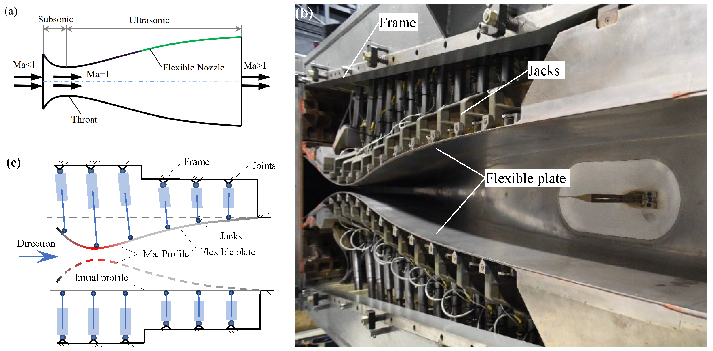
2.1.1. Structural Components and Working Principle of the Flexible Nozzle

The schematic and physical drawings of a typical flexible wall nozzle are presented in Figure 1a,b, which illustrate the main components, including the flexible plate, driving rod, frame, etc. The fundamental concept is to leverage the expansion and contraction of the driving rod to drive the flexible plate to bend and mold in a manner that produces the desired aerodynamic profile curve. The appearance of the flexible wall nozzle not only enhances the efficiency of the test, but also increases the likelihood of modifying the Mach number during the test, which expands the capabilities of the wind tunnel for testing and represents a significant area of focus for trans-supersonic wind tunnel research.

As illustrated in Figure 1c, the flexible plate was initially configured as a flat plate. During operation, the actuator rod exerted a force on the flexible plate, causing it to deform elastically and form nozzle profiles with varying Mach numbers. As the flexible plate deformed, the drive rod itself rotated around a hinge point on the frame in order to accommodate the constraint of constant arc length of the flexible plate. The drive rod of the flexible wall nozzle is typically a hydraulic cylinder or an electric actuator, which is usually equipped with a linear displacement sensor for closed-loop position and velocity control. The elastic deformation of the flexible plate after the formation of the throat (the narrowest point) was significantly larger than the thickness of the plate, which is a notable departure from the large deflection deformation problem observed in typical rectangular thin plates.

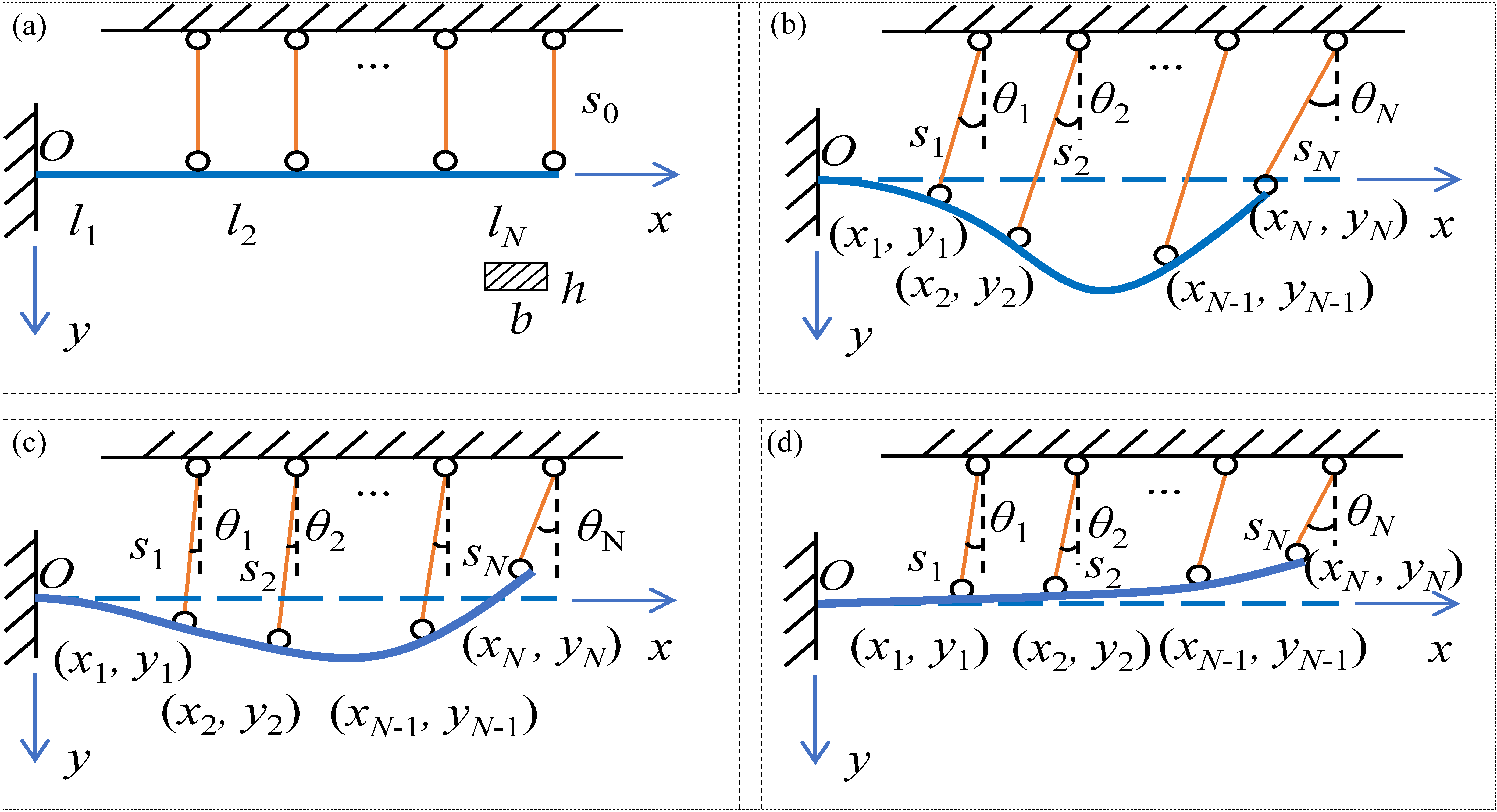
2.1.2. The Mechanical Model of the Flexible Nozzle

For the multi-point flexible wall nozzle, its main bending direction can be expressed as an elastic beam with multi-point support. In essence, the beam model approximation was justified because the nozzle wall’s geometry (which had a long, thin structure) and deformation characteristics aligned well with classical beam theory assumptions, allowing us to effectively analyze its mechanical behavior while maintaining computational efficiency. Figure 2 shows the deformation schematic of the multi-point supported elastic beam, where Figure 2a is the initial state, Figure 2b–d are the state with all elongation, elongation with shortening, and all contraction, respectively. The left side is the fixed point, and the right side is the free end, which was divided into N segments in total. The supports are physical connection points between the flexible plate (beam) and the driving rods, allowing precise shape control at discrete locations along the plate length.

Under the three deformation conditions, the rotation phenomenon occurred in each driving rod, and the rotation angle was related to the deformation scale of the beam. In order to facilitate the establishment of the mathematical model of the multi-point supported elastic beam, the coordinate system XOY was established with the fixed end of the beam as the origin, the direction along the axis of the elastic beam as the x-axis, and the normal direction as the y-axis. The flexible plate undergoes large deflection deformation under the action of elongation or shortening of the driving rod, and this causes the driving rod to rotate. Although it can be simplified as an elastic beam problem, this process still involves complex mechanical problems. On the one hand, there is a geometrically nonlinear deformation of the flexible structure with large deflection, and, on the other hand, there is a kinematic coupling relationship between the driving rod and the elastic beam. Therefore, with only the boundary constraints of the driving rod, the mechanism also has a multi-solution problem, which further increases the difficulty of solving this problem. It can be seen that the essence of multi-point-supported elastic beam deformation is a large deflection beam deformation problem under multi-point dynamic constraints.

2.1.3. Model Solving Based on the Variational Principle

As shown in Figure 2, the initial length of each support rod is $S_0$, the length of each beam segment is $l_1, l_2, \dots ,l_N$, the width of the beam is b, and the thickness is h. The elongation of each support rod is $S_1, S_2, \dots ,S_N$, the support angle changes after the elongation of the rod is ${\theta }_1, {\theta }_2, \dots ,{\theta }_N$, and the coordinates of each support point are $(x_1,y_1)$ … $(x_N,y_1)$… $(x_N,y_1)$… $(x_N,y_1)$ … $(x_N,y_N)$. The boundary conditions for the multi-point-supported elastic beam problem are

$$\left\{\begin{array}{c}{\int }_{x_{i-1}}^{x_i}(\sqrt{1+{w^{\prime }}^2}dx-l_i)=0\hfill \\ x_i=\sum _{n=1}^i(l_i-(s_i+s_0)sin{\theta }_i)(i=1,2,3,\cdots ,n)\hfill \\ y_i=\left(s_0+s_i\right)cos{\theta }_i-s_0\hfill \\ w\left(x_i\right)=y_i\hfill \\ w^{″}\left(x_i\right)\ne 0\hfill \end{array}\right.,$$

(1)

where w represents the deflection, while $w^{\prime }$ and $w^{″}$ denote its first and second derivatives, respectively. As illustrated in Figure 2, $s_i$ represents the increased length of the driving rod, and $s_0$ indicates its initial length. The first line of Equation (1) expresses the conservation of the arc length during deformation. The final line of Equation (1) indicates that a non-zero bending moment exists at the support point.

According to the energy principle, the true deformation of the beam will cause the deformation energy to take a very small value under the constraint that the beam is guaranteed to be inextensible. In turn, the solution is carried out by the variational principle. To obtain the shape function in the minimum energy state, the generalized function with constraints is

$$\Pi ={\int }_0^{x_N}{\displaystyle \frac{1}{2}}EI{\left[{\displaystyle \frac{w^{″}}{{\left(1+w^2\right)}^{\frac{3}{2}}}}\right]}^{2}dx+\sum _{i=1}^N{\lambda }_i\left({\int }_{x_{i-1}}^{xi}\sqrt{1+{w^{\prime }}^2}dx-l_i\right),$$

(2)

where ${\lambda }_i$ (i = 1, 2) is the Raschner multiplier, whose exact value is determined by the boundary conditions and variational constraints. Variational differentiation of the generalized function of the above equation, i.e., $\delta \Pi =0$, yields

$$\begin{array}{c}EI\sum _{i=1}^N\left[{\int }_{x_{i-1}}^{x_i}\left({\displaystyle \frac{3w^{\prime }{w^{\prime }}^2}{{\left(1+{w^{\prime }}^2\right)}^4}}-{\displaystyle \frac{w^{‴}}{{\left(1+{w^{\prime }}^2\right)}^3}}+{\displaystyle \frac{{\lambda }_i}{EI}}{\displaystyle \frac{w^{\prime }}{\sqrt{1+{w^{\prime }}^2}}}\right)\delta w^{\prime }dx+\delta {\lambda }_i\left({\int }_{x_{i-1}}^{x_i}\sqrt{1+{w^{\prime }}^2}dx-l_i\right)\right]\\ =0(i=1,2,\dots ,N).\end{array}$$

(3)

This yields the Euler–Lagrange equations and constraints as

$$\begin{array}{c}{\displaystyle \frac{3w^{\prime }{w^{″}}^2}{{\left(1+{w^{\prime }}^2\right)}^4}}-{\displaystyle \frac{w^{‴}}{{\left(1+{w^{\prime }}^2\right)}^3}}+{\displaystyle \frac{{\lambda }_i}{EI}}{\displaystyle \frac{w^{\prime }}{\sqrt{1+{w^{\prime }}^2}}}=0(i=1,2,\dots ,N)\\ {\int }_{x_{i-1}}^{x_i}\sqrt{1+{w^{\prime }}^2}dx-l_i=0(i=1,2,\dots ,N).\end{array}$$

(4)

Solving the Euler–Lagrange equation can obtain the general solution of the shape function, and the specific form of the shape function can be determined according to the boundary conditions and constraints. It is worth noting that the Euler equation here implies the influence of each segment of the strut on each other. Although it is solved segment by segment, it is also considered as a whole and the accuracy of the results is guaranteed.

The Taylor series expansion uses the starting point of each beam section as the expansion point. This allows us to accurately represent the beam’s deformation behavior by expanding around local reference points, making the calculations more tractable while maintaining precision in describing the geometric nonlinearity of the flexible structure. The Euler–Lagrange equations are solved in the form of Taylor series expansion, and the solution form is as follows:

$$w=w\left(x_0\right)+w^{\prime }\left(x_0\right)\left(x-x_0\right)+{\displaystyle \frac{w^{″}\left(x_0\right)}{2!}}{\left(x-x_0\right)}^2+{\displaystyle \frac{w^{‴}\left(x_0\right)}{3!}}{\left(x-x_0\right)}^3+\cdots$$

(5)

At the starting end, the function value and first-order derivative can be determined from either the initial endpoint’s boundary value or the previous beam section’s results. While the second-order derivative remains unknown, the third-order and higher-order functions can be expressed in terms of the second-order derivative function using Euler’s formula:

$$w^{‴}={\displaystyle \frac{3w^{\prime }{w^{″}}^2}{1+{w^{\prime }}^2}}+{\displaystyle \frac{\lambda }{EI}}{w}^{\prime }{\left(1+{w^{\prime }}^2\right)}^{\frac{5}{2}},$$

(6)

$$w^{\left(4\right)}={\displaystyle \frac{3{w^{″}}^3\left(1+5{w^{\prime }}^2\right)}{{\left(1+{w^{\prime }}^2\right)}^2}}+{\displaystyle \frac{\lambda }{EI}}{w}^{″}{\left(1+{w^{\prime }}^2\right)}^{\frac{1}{2}}\left(12{w^{\prime }}^4+13{w^{\prime }}^2+1\right),$$

(7)

$$w^{\left(5\right)}={\displaystyle \frac{15w^{\prime }{w^{″}}^{4\left(7{w^{\prime }}^2+3\right)}}{{\left(1+{w^{\prime }}^2\right)}^3}}+{\displaystyle \frac{\lambda }{EI}}{\displaystyle \frac{3w^{\prime }{w^{″}}^2}{{\left(1+{w^{\prime }}^2\right)}^{\frac{1}{2}}}}\left(47{w^{\prime }}^4+60{w^{\prime }}^2+13\right)+\cdots$$

(8)

The generalized solution obtained above contains two unknown quantities, the value of the second-order derivative and the Raschner multiplier, which need to be determined in the below equation by means of the boundary conditions at the right endpoint of each beam segment. The system of equations to be solved is as follows:

$$\left\{\begin{array}{c}{\int }_{{\overline{x}}_{i-1}}^{{\overline{x}}_i}\sqrt{1+{w^{\prime }}^2}dx-l_i=0\hfill \\ {\overline{x}}_i=\sum _{n=1}^i{l}_n-\left(s_0+s_i\right)sin\theta (i=1,2,\dots ,N)\hfill \\ {\overline{y}}_i=\left(s_0+s_i\right)cos\theta -s_0\hfill \\ w\left({\overline{x}}_i\right)={\overline{y}}_i\hfill \\ w^{\prime }\left({\overline{x}}_i\right)={\alpha }_i\hfill \end{array}\right..$$

(9)

The above calculations are carried out for each beam segment, and the complete deformation curve of a multi-point-supported elastic beam is determined after obtaining the solutions for all segments.

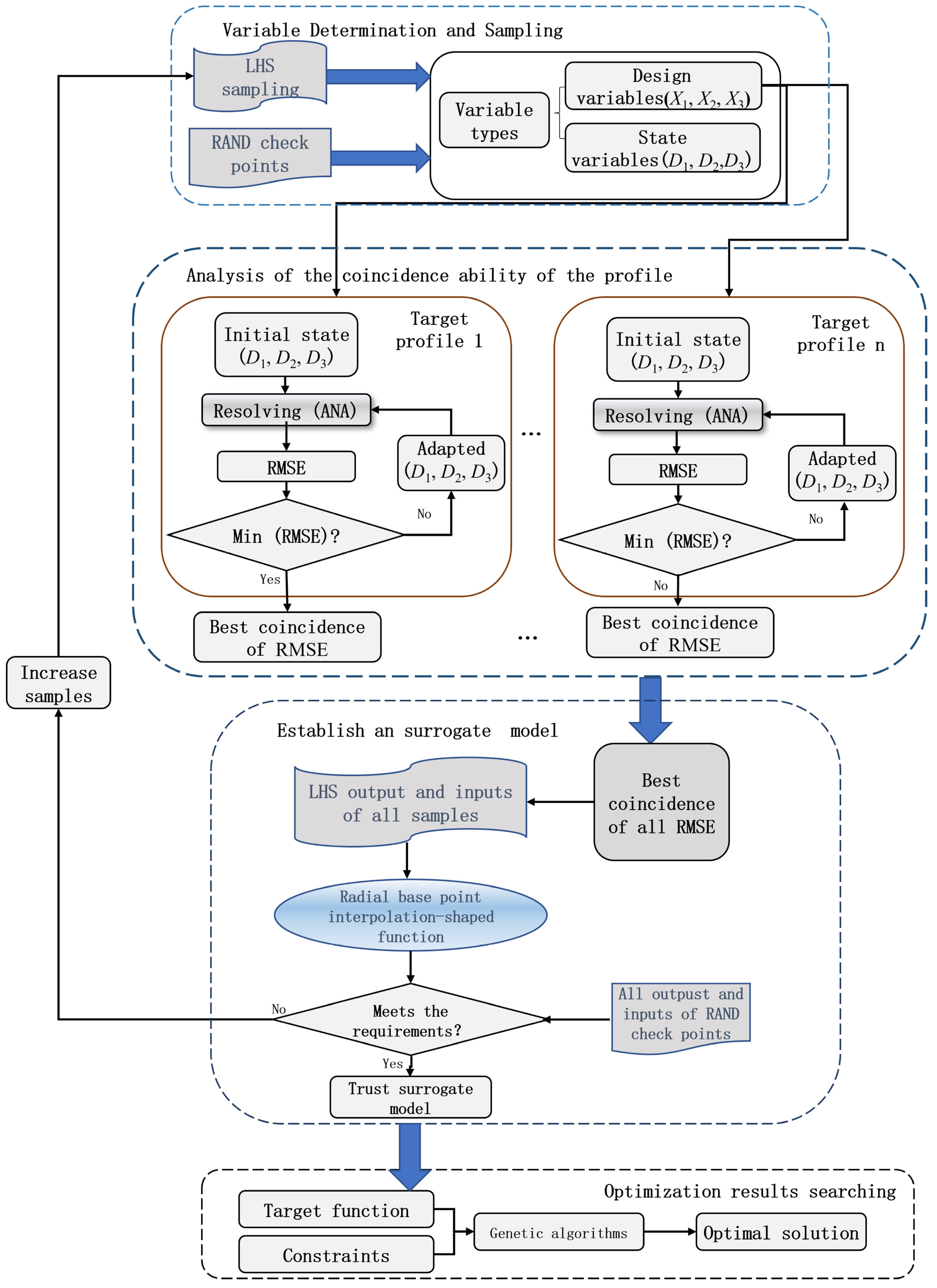
2.2. Optimization Design Based on Radial Basis Interpolation of Surrogate Models

2.2.1. Basic Definition of the Radial Point Interpolation Method

The radial point interpolation method (RPIM) combines the point interpolation method (PIM) and the radial base function (RBF), which have been widely used in meshless simulations and other fields. RPIM provides an efficient way to create accurate surrogate models for complex engineering problems by enabling the interpolation of scattered data points without requiring a structured grid. The method is particularly valuable for optimizing the flexible nozzle design as it can handle multiple design variables, non-linear relationships between inputs and outputs, and complex geometric constraints. This approach significantly reduces the computational cost compared to full numerical simulations while maintaining accuracy. The following equation describes RPIM as

$$u^h\left(\mathbf{x}\right)=\sum _{i=1}^n{R}_i\left(\mathbf{x}\right)a_i={\mathbf{R}}^{\mathbf{T}}\left(\mathbf{x}\right)\mathbf{a},$$

(10)

where $R_i(\mathbf{x}$) is the radial basis function. The RPIM interpolation with polynomial expansion is expressed as

$$u\left(\mathbf{x}\right)=\sum _{i=1}^n{R}_i\left(\mathbf{x}\right)a_i+\sum _{j=1}^m{P}_j\left(\mathbf{x}\right)b_j={\mathbf{R}}^{\mathbf{T}}\left(\mathbf{x}\right)\mathbf{a}+{\mathbf{P}}^{\mathbf{T}}\left(\mathbf{x}\right)\mathbf{b},$$

(11)

where $P_j\left(x\right)$ is the polynomial basis term in the spatial coordinates x; n and m denote the number of RBFs and the number of polynomial basis terms, respectively; $a_i$ and $b_j$ are the unknown coefficients; $R_i\left(x\right)$ denotes the RBF with the variable r; and r denotes the distance between the point x and the node $x_i$.

$$r=\sqrt{{(x-x_i)}^2+{(y-y_i)}^2}.$$

(12)

To determine the unknown coefficients $a_i$ and $b_j$ in Equation (10), the a support domain containing n field nodes is created at point x. The state function values of the n-sampled nodes are described in vector form as

$${\mathbf{U}}_{\mathbf{S}}={\mathbf{R}}_{\mathbf{0}}\mathbf{a}+{\mathbf{P}}_{\mathbf{m}}\mathbf{b}.$$

(13)

In addition, m additional equations are as follows:

$${{\mathbf{P}}_{\mathbf{m}}}^{\mathbf{T}}\mathbf{a}=\mathbf{0}.$$

(14)

Combining Equations (13) and (14) yields

$${\tilde{\mathbf{U}}}_s=\left[\begin{array}{c}{\mathbf{U}}_{\mathbf{s}}\\ \mathbf{0}\end{array}\right]=\left[\begin{array}{cc}{\mathbf{R}}_{\mathbf{0}}& {\mathbf{P}}_{\mathbf{m}}\\ {\mathbf{P}}_{\mathbf{m}}^{\mathbf{T}}& \mathbf{0}\end{array}\right]\left\{\begin{array}{c}\mathbf{a}\\ \mathbf{b}\end{array}\right\}=\mathbf{G}{\mathbf{a}}_{\mathbf{0}},$$

(15)

where

$$\mathbf{G}=\left[\begin{array}{cc}{\mathbf{R}}_{\mathbf{0}}& {\mathbf{P}}_{\mathbf{m}}\\ {{\mathbf{P}}_{\mathbf{m}}}^{\mathbf{T}}& \mathbf{0}\end{array}\right].$$

(16)

Equation (10) at point x is then expressed as

$$u\left(\mathbf{X}\right)={\tilde{\mathbf{\Phi }}}^T{\tilde{\mathbf{U}}}_s=\left\{{\mathbf{R}}^{\mathbf{T}}\left(\mathbf{x}\right){\mathbf{P}}^{\mathbf{T}}\left(\mathbf{x}\right)\right\}{\mathbf{G}}^{-\mathbf{1}}{\tilde{\mathbf{U}}}_s,$$

(17)

where ${\tilde{\mathbf{\Phi }}}^T$ is the node displacement corresponding to the first n components of the shape function derived from RPIM:

$${\tilde{\mathbf{\Phi }}}^T=\{{\varphi }_1\left(\mathbf{x}\right){\varphi }_2\left(\mathbf{x}\right)\cdots \left.{\varphi }_{n+m}\left(\mathbf{x}\right)\right\}.$$

(18)

Thus, Equation (17) is reformulated as

$$u\left(\mathbf{x}\right)={\mathbf{\Phi }}^{\mathbf{T}}\left(\mathbf{x}\right){\mathbf{U}}_{\mathbf{S}}=\sum _{i=1}^n{\varphi }_i{u}_i.$$

(19)

Notice that the ${\mathbf{\Phi }}^{\mathrm{T}}\left(\mathbf{x}\right)$ is called the shape function corresponding to the displacement of the node.

$${\mathbf{\Phi }}^{\mathrm{T}}\left(\mathbf{x}\right)=\left\{\begin{array}{ccc}{\varphi }_1\left(\mathbf{x}\right)\hfill & {\varphi }_2\left(\mathbf{x}\right)\hfill & \cdots \hfill \end{array}{\varphi }_n\left(\mathbf{x}\right)\right\}.$$

(20)

The shape function ΦT(x) is a mathematical function that determines how the surrogate model interpolates between known data points. It acts as a weighting function that defines how much influence each sample point has on the prediction at any given location in the design space. Φ$\left(x\right)$ represents the contribution of the i-th sample point to the prediction at location x. The shape function combines these individual contributions to create a continuous prediction surface across the design space. By carefully constructing these shape functions, RPIM can accurately approximate the complex relationships between design variables (inputs) and performance metrics (outputs).

2.2.2. Evaluation Index for the Accuracy of the Nozzle Profile

The flexible plate’s elastic curve is formally characterized by a series of straight lines between the support points [10]. These straight lines can be overlapped in the curvature diagram of the pneumatic profile, which is a graphical representation of the curve’s shape and position. The diagram also encompasses an area that represents the elastic curve and the theoretical curve between the coincident error. The smaller the enclosed area, the more accurate the fit. The optimal method for determining the precise area is to employ the integration method, whereby the position of the support point with the smallest encircled area is identified as the optimal position.

It should be noted that not all aerodynamic curves are able to be obtained using a continuous slope curve. In the case of a known aerodynamic profile, the curve resulting from the two differentials is frequently discontinuous, thereby making it challenging to accurately evaluate the degree of profile fit using a curvature curve.

In addition to the curvature deviation, the deviation of the elastic curve from the aerodynamic contour at the corresponding position of the support point can also be used as an evaluation index. This reflects the accuracy of the profile overlap more intuitively. However, the position of the driving point does not reflect the degree of overlap of the complete surface. Furthermore, this method has certain limitations. The root mean square error (RMSE) is a comprehensive measure that accounts for all the discrepancies between the observed data and the theoretical curves. This approach allows for a more precise characterization of the degree of overlap between the actual profile and the aerodynamic contour across the entire profile. Consequently, this study proposes the use of RMSE as a profile evaluation index.

$$R=\sqrt{{\displaystyle \frac{\sum {\left(Y_i-Y_i^{\prime }\right)}^2}{N}}},$$

(21)

where $Y_i$ is the measured profile coordinates of the ith point, ${Y_i}^{\prime }$ is the theoretical profile coordinates of the ith point, and N is the total number of points involved in the calculation.

2.2.3. Optimizing the Design Process

The sum of the root mean square deviations corresponding to the n Mach number patterns is used as the objective function for optimization. And the constraints are m-section flexure plate length limits.

$$G_{obj}=\sum _1^{n}RMSE,$$

(22)

$$L_{max}{>X}_m>L_{min},$$

(23)

where $L_{min}$ is the minimum length of the given flexible ledge, and $L_{max}$ is the maximum length of the given flexible ledge.

The optimization process of the multi-point flexible wall nozzle structure is illustrated in Figure 3. This process comprises four principal stages: (1) variable determination and sampling point selection, (2) analysis of the corresponding profile overlap of sampling points, (3) establishment of the surrogate model, and (4) identification of the optimal result through the use of the surrogate model.

(1) Determination of Variables and the Selection of Sampling Points

To ensure precise control of the flexible pneumatic structure’s shape, we must determine each structural parameter and select support point positions as design variables. The value range and sampling space of these design variables must align with the actual structure. Initially, we determined the number of sampling points and used the Latin hypercube sampling method to sample the space. We then employed the random sampling function rand() to select the specified number of test points.

(2) Sampling Points Corresponding to the Profile Overlap Analysis

We defined the initial driving quantity as the y-coordinate, where the pneumatic profile’s arc length equals the spacing between driving points, and we then determined the solution range for each driving point.

Using the nozzle flexible plate’s large deflection deformation analytical solution method, we obtained an elastic curve solution. By comparing this with the pneumatic theoretical contour, we calculated the root mean square error of the profile—our optimization objective. We performed this optimization process on N theoretical profiles, calculated their root mean square errors, and then aggregated these errors to obtain the final sampling point results.

(3) Establishment of the Surrogate Model

We verified the surrogate model’s accuracy using the shape function and checkpoints. If specifications were not met, we increased the number of sampling points.

(4) Optimizing the Surrogate Model

We used the Python Optimization Toolbox’s “Optimization Tool” to find the optimal solution for the surrogate model. Specifically, we employed the genetic algorithm (GA), which offers efficient, parallel, and global search capabilities. The GA automatically acquires and accumulates search space knowledge while adaptively controlling the search process to find the optimal solution, effectively avoiding the local optima during optimization.

3. Results

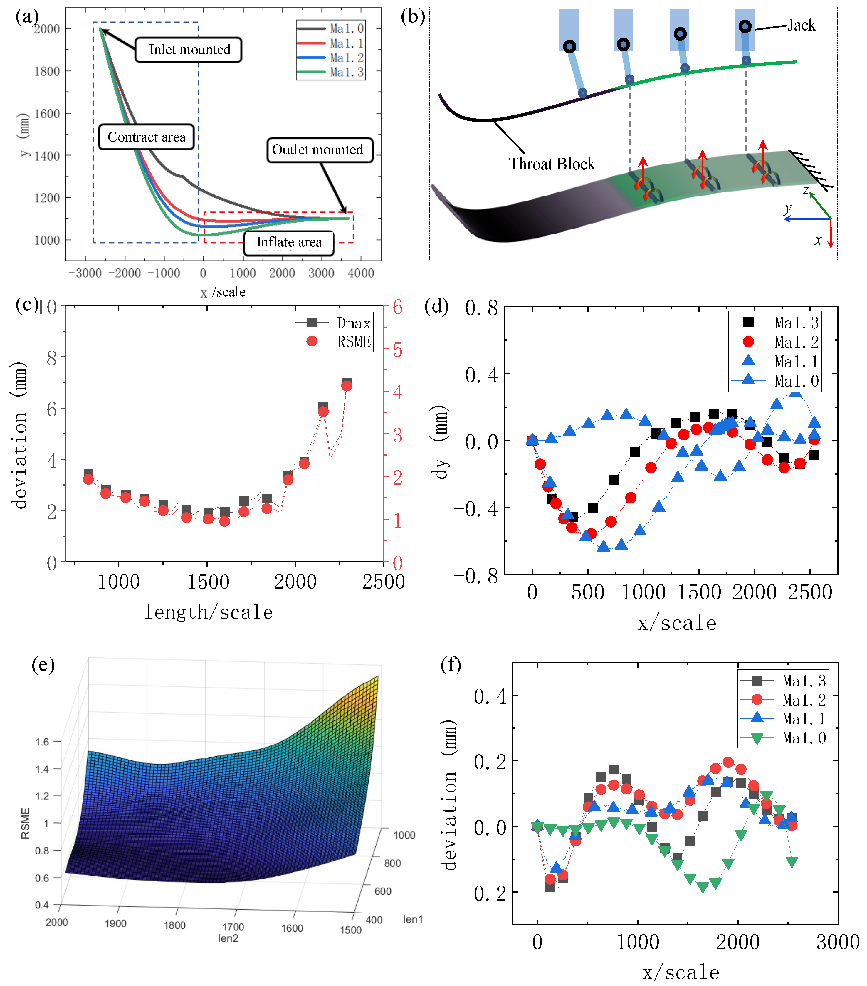
3.1. The Optimization Results

The optimization object is a large wind tunnel nozzle section, and four types of Mach number profiles, with values of 1.3, 1.2, 1.1, and 1.0, were designed. The aerodynamic contours are illustrated in Figure 4a,b, wherein the Mach number 1.0 represents a contraction curve, while the remaining profiles depict contraction–expansion curves. The aerodynamic profile is divided into two regions, which are delineated by the throat and serve as the demarcation point. The inlet to the throat is designated as the contraction region, while the throat to the outlet is classified as the expansion region. Of particular note is the expansion region, which presents a significant challenge in terms of the elastic profile required for the flexible plate. This is a crucial aspect of the structural design.

In order to ensure profile accuracy, the structure of the flexible wall nozzle is subjected to a rigorous calculation and analysis process. On this basis, the profile deviations, corresponding to the two cases of downstream setting of a single-group driving mechanism and a two-group driving mechanism, are compared in order to determine the final number and position of the driving points.

(1) Single-group driving jacks

Figure 4c gives the curve of the influence of the position of the single-group drive mechanism drive on the profile reclamping accuracy and the root mean square deviation, from which it can be seen that the largest profile deviation had the same trend as the root mean square deviation, and the optimal design point was located near x = 1600.

Once the location of the driving point was determined, the corresponding four Mach number faced deviations, as illustrated in Figure 4d. The largest profile deviation was observed in the vicinity of the coordinate origin at a distance of approximately 750, for the Mach 1.1 condition, with a magnitude of −0.7 mm. The largest deviation for the Mach 1.1, 1.2, and 1.3 profiles was observed between the drive point and the fixed point. This was due to the fact that there was a slight change in the angle of the aerodynamic theoretical curve at this position, which was not accounted for by the structure’s fixed connection. The profile exhibiting the greatest degree of overlap was that corresponding to Mach 1.0, with a maximum deviation of approximately 0.3 mm. However, the deviations observed in all four of the Mach profiles exceeded the ±0.2 mm threshold specified in the design specifications. This finding suggests that a single drive point is insufficient to meet the design requirements.

(2) Double-group driving jacks

The x-coordinate ranges of the two drive points were determined to be [400, 1000] and [1500, 2000], respectively, based on the influence of factors, such as the spacing between the drive mechanism and the drive mechanism, as well as the spacing between the drive mechanism and the frame. Subsequently, the Latin hypercubic sampling method was employed to obtain the sampling points and to calculate the root mean square deviation sum of all the Mach number-type surfaces. Thereafter, the feasible interval surface was plotted using the RPIM method, as illustrated in Figure 4e. As illustrated in the figure, the global optimum point was situated in close proximity to the boundary. Furthermore, the RSME exhibited minimal variation in the vicinity of the optimum point. Consequently, the structural size could be determined in the region in accordance with the engineering reality. The x-coordinate of the driving point was ultimately selected to be 500 and 1750, respectively. Figure 4f depicts the overlap deviation of the four Mach profile surfaces following optimization. The maximum deviation was approximately −0.19 mm, which satisfies the ±0.2 mm accuracy requirement.

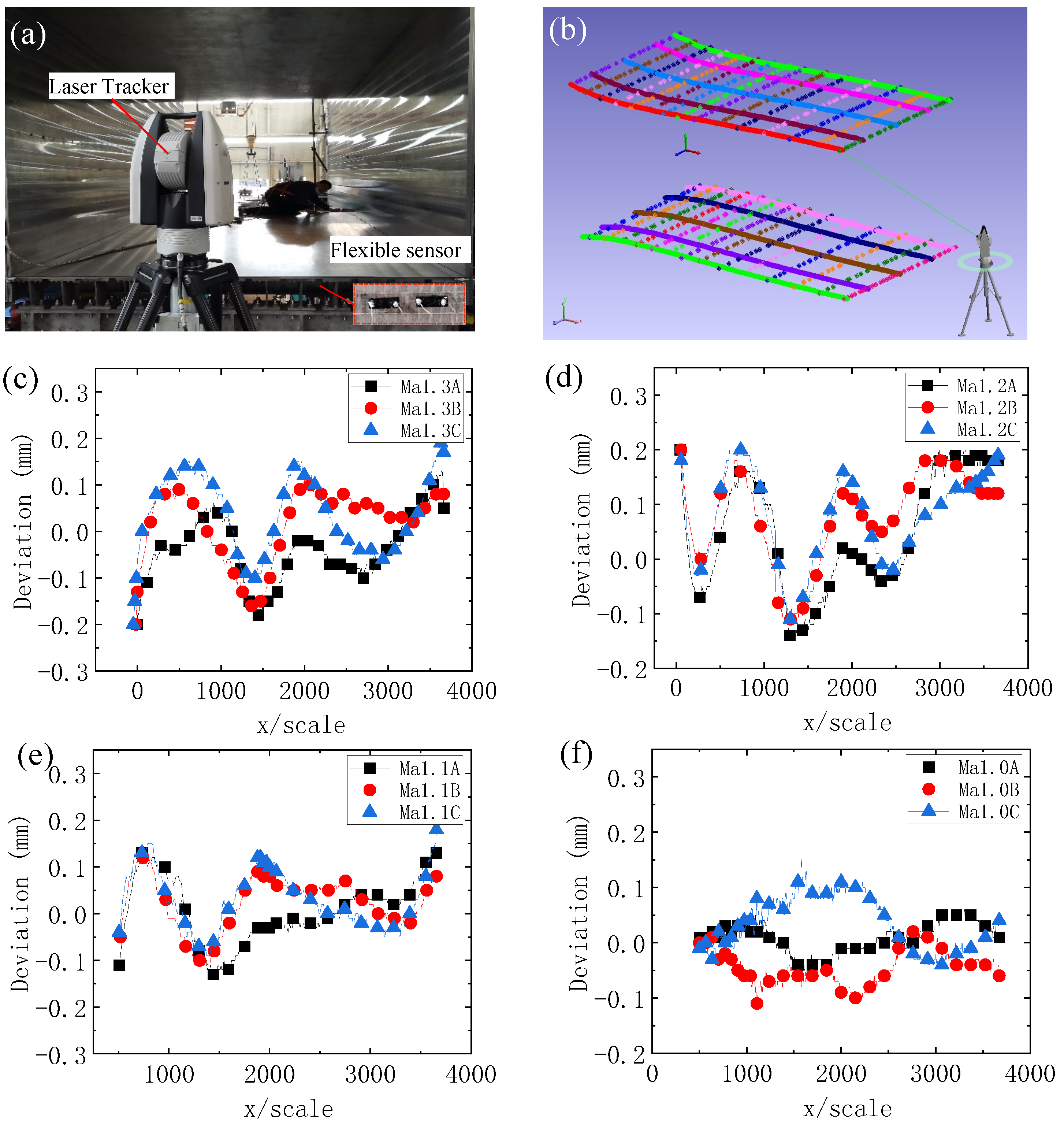
3.2. Experimental Results

The width of the flexible wall nozzle prototype was 2600, which is considerable for a flexible wall nozzle. To ensure an accurate evaluation of the nozzle profile, five curves were selected for measurement and analysis along the width direction. The middle three curves were subsequently utilized as the final evaluation curves. Additionally, 21 cross-sections were selected along the wind tunnel axis to assess the deformation of the flexible plate in the width direction, which was employed to evaluate the molding effect of the profile. Figure 5a depicts the photograph of the site, where the laser tracker operator conducted measurements within the nozzle, while Figure 5b illustrates the meshed curves obtained from the laser tracker measurements and the flexible sensors. As illustrated in the figure, the middle three curves along the axial direction were capable of encompassing the nozzle profile within the core region of the flow field.

Figure 5c–f illustrate the outcomes of the profile deviation for the four profiles with the Mach numbers of 1.3, 1.2, 1.1, and 1.0, respectively. In this illustration, B represents the middle cross-section curve, and A and C are the two side cross-section curves. The measurement results demonstrate that the profile deviation downstream of all Mach number throats can meet the index requirement of ±0.2 mm, thereby verifying the feasibility of the structural optimization design and shape control method studied in this paper.

4. Discussion

4.1. Scalability Considerations

When scaling to larger and more complex nozzle configurations, several challenges emerge. The dimensionality of the optimization problem increases substantially with each additional control point, leading to a more complex solution space. For configurations with more than eight control points, we found that the computational time could extend beyond practical limits, necessitating alternative approaches or computational strategies.

4.2. Model Accuracy vs. Computational Cost Trade Offs

Our analysis revealed several important trade offs between the model accuracy and computational efficiency. Higher-fidelity models provide better accuracy but require significantly more computational resources. Simplified surrogate models can reduce the computation time by 60–70% while maintaining acceptable accuracy (within ±0.2 mm). And the optimal balance point appeared to be achieved when using medium-fidelity models during optimization, followed by high-fidelity validation of the final solutions.

These findings suggest that, while our approach is highly effective for current applications, future work should focus on developing more efficient optimization algorithms and exploring advanced parallel computing strategies to handle increasingly complex nozzle configurations.

5. Conclusions

This paper achieved several significant results in flexible aerodynamic structure optimization. We successfully developed and validated a mathematical model for large deflection deformation of multi-pivot flexible walled nozzles based on the variational principle, implemented an efficient surrogate model using radial basis interpolation for structural optimization, and demonstrated its effectiveness through experimental validation. Our wind tunnel tests confirmed remarkable precision, achieving shape surface accuracy within ±0.2 mm under operational conditions. This proven methodology not only solves the immediate challenge of flexible nozzle optimization, but also establishes a practical framework for shape control and structural optimization in various flexible aerodynamic applications, including intelligent deformed wings and variable engine nozzles.

References

1. Bin, X.U.; Shi, Z. An overview on flight dynamics and control approaches for hypersonic vehicles. Sci. China Inf. Sci. 2015, 58, 1–19. [Google Scholar] [CrossRef]
2. Jingyi, W.U.; Wang, M.; Wang, S. Numerical Wind Tunnel Study of Semi-Open Silo Shell Grids. J. Beijing Univ. Civ. Eng. Archit. 2024, 40, 84–92. [Google Scholar] [CrossRef]
3. Chen, X.; Li, C.; Gong, C.; Guo, L.; Da, R.A. A study of morphing aircraft on morphing rules along trajectory. Chin. J. Aeronaut. 2021, 34, 232–243. [Google Scholar] [CrossRef]
4. Marwege, A.; Kirchheck, D.; Klevanski, J.; Gülhan, A. Hypersonic retro propulsion for reusable launch vehicles tested in the H2K wind tunnel. CEAS Space J. 2022, 14, 473–499. [Google Scholar] [CrossRef]
5. Yu, C.; Gao, X.; Liao, W.; Zhang, Z.; Wang, G. A Highly Accurate Method for Deformation Reconstruction of Smart Deformable Structures Based on Flexible Strain Sensors. Micromachines 2022, 13, 910. [Google Scholar] [CrossRef]
6. Aboelezz, A.; Mohamady, O.; Hassanalian, M.; Elhadidi, B. Nonlinear Flight Dynamics and Control of a Fixed-Wing Micro Air Vehicle: Numerical, System Identification and Experimental Investigations. J. Intell. Robot. Syst. 2021, 101, 173–186. [Google Scholar] [CrossRef]
7. Vijayakrishnan, V.; Kishore, P.; Muruganandam, T.M. Investigation of Variable Mach Number Wind Tunnel with Symmetric Sliding Block Nozzles. In Proceedings of the AIAA Scitech 2022 Forum, San Diego, CA, USA, 3–7 January 2022; Volume 13, p. 0716. [Google Scholar] [CrossRef]
8. Edquist, K.T. Status of Mars Retropropulsion Testing in the Langley Unitary Plan Wind Tunnel. In Proceedings of the AIAA Scitech 2022 Forum, San Diego, CA, USA, 3–7 January 2022; p. 0911. [Google Scholar]
9. Sabnis, K.; Babinsky, H.; Galbraith, D.S.; Benek, J.A. Nozzle geometry-induced vortices in supersonic wind tunnels. AIAA J. 2020, 59, 1087–1098. [Google Scholar] [CrossRef]
10. Yu, C.; Li, Z.; Zhang, Z.; Meng, L.; Wang, G.; Shi, Y.; Gao, C. A mechanics model in design of flexible nozzle with multiple movable hinge boundaries. Heliyon 2023, 9, e12927. [Google Scholar] [CrossRef] [PubMed]
11. Wu, X.; Zhang, W.; Song, S. Uncertainty Quantification and Sensitivity Analysis of Transonic Aerodynamics with Geometric Uncertainty. Int. J. Aerosp. Eng. 2017, 2017, 1–16. [Google Scholar] [CrossRef]
12. Ross, J.C.; Rhode, M.N. Evaluation of CFD as a Surrogate for Wind-Tunnel Testing for Mach 2.4 to 4.6—Project Overview. In Proceedings of the AIAA AVIATION 2021 FORUM, Virtual, 2–6 August 2021; p. 2961. [Google Scholar] [CrossRef]
13. Chucheepsakul, S.; Phungpaigram, B. Elliptic integral solutions of variable-arc-length elastica under an inclined follower force. J. Appl. Math. Mech. 2020, 84, 29–38. [Google Scholar] [CrossRef]
14. Yuan, W.H.; Wang, H.C.; Zhang, W.; Dai, B.B.; Wang, Y. Particle finite element method implementation for large deformation analysis using Abaqus. Acta Geotech. 2021, 16, 2449–2462. [Google Scholar] [CrossRef]
15. Qiang, W.U.; Peng, P.; Cheng, Y. The interpolating element-free Galerkin method for elastic large deformation problems. Sci. China Technol. Sci. 2021, 64, 364–374. [Google Scholar] [CrossRef]
Figure 1. (a) The principle of a nozzle in spline style. The arrows denote the flow speeds with directions where they locate. (b) A typical picture of the flexible nozzle plate of a wind tunnel. (c) The schematics of the flexible nozzle plate of the wind tunnel of (b).
Applsci 15 03169 g001
Figure 2. (a) The initial state of the elastic beam with multi-point supports. (bd) The states of all elongation, elongation with shortening, and all contraction, respectively.
Applsci 15 03169 g002
Figure 3. The optimization process of the multi-point flexible wall nozzle structure. The optimization process consists of four steps: (1) define the variables and select sampling points using the Latin hypercube method, (2) analyze the profile overlap by calculating elastic curves and comparing them with theoretical profiles, (3) build and validate the surrogate model using shape functions, and (4) optimize using the genetic algorithm to find the global solution.
Applsci 15 03169 g003
Figure 4. Optimization and analysis of the flexible nozzle design: (a) Theoretical profiles for the four different Mach numbers (1.3, 1.2, 1.1, and 1.0) showing the target shapes. (b) Schematic representation of the nozzle plate structure illustrating the key components and dimensions. (c) Analysis of the drive mechanism position impact on the profile accuracy, showing the root mean square deviation versus the drive point location. (d) Profile deviation analysis for all the four Mach numbers after optimal drive point placement. (e) The three-dimensional feasible solution space visualization generated using RPIM interpolation. (f) Comparative analysis of the profile surface deviations post-optimization for all the four Mach number configurations.
Applsci 15 03169 g004
Figure 5. Experimental validation of the flexible nozzle design through detailed measurements and comparisons. (a) The experimental setup of the laser tracker measurement process inside the nozzle, highlighting our rigorous data collection methodology. (b) The high-resolution mesh curves obtained from both laser tracker measurements and flexible sensors, providing comprehensive shape data. (cf) Detailed profile deviation analyses for each of the Mach number configurations (1.3, 1.2, 1.1, and 1.0, respectively), allowing for a quantitative assessment of our design’s performance against theoretical predictions. The results demonstrate strong agreement between the designed and achieved profiles, with deviations falling within acceptable engineering tolerances.
Applsci 15 03169 g005
Disclaimer/Publisher’s Note: The statements, opinions and data contained in all publications are solely those of the individual author(s) and contributor(s) and not of MDPI and/or the editor(s). MDPI and/or the editor(s) disclaim responsibility for any injury to people or property resulting from any ideas, methods, instructions or products referred to in the content.