Fiber Sensing in the 6G Era: Vision Transformers for ϕ-OTDR-Based Road-Traffic Monitoring

Abstract

This article adds to the emergent body of research that examines the potential of 6G as a platform that can combine wired and wireless sensing modalities. We apply vision transformers (ViTs) in a distributed fiber-optic sensing system to evaluate road traffic parameters in smart cities. Convolutional neural networks (CNNs) are also assessed for benchmarking. The experimental setup is based on a direct-detection phase-sensitive optical time-domain reflectometer ($\varphi$-OTDR) implemented using a narrow linewidth source. The monitored fibers are buried on the university campus, creating a smart city environment. Backscattered traces are consolidated into space–time matrices, illustrating traffic patterns and enabling analysis through image processing algorithms. The ground truth is established by traffic parameters obtained by processing video camera images monitoring the same street using the YOLOv8 model. The results indicate that ViTs outperform CNNs for estimating the number of vehicles and the mean vehicle speed. While a ViT necessitates a significantly larger number of parameters, its complexity is similar to that of a CNN when considering multiply–accumulate operations and random access memory usage. The processed dataset has been made publicly available for benchmarking.

1. Introduction

It is envisioned that 6G will bring about a revolution in how we connect, communicate, and interact with the world. Artificial intelligence (AI) will be natively integrated into 6G systems to enable them to be smarter and more responsive [1]. Moreover, the integration of sensing into wireless communication systems, known as integrated sensing and communications (ISAC) [2] or joint communication and sensing (JCAS) [3], will allow 6G devices to progress beyond communication. ISAC will allow 6G devices to sense their surroundings for real-time applications such as autonomous driving and healthcare monitoring [4]. While much of the current research in this area focuses on the “wireless” medium for joint/integrated communication and sensing, this manuscript contributes to an expanded approach for 6G that also incorporates a “wired” medium infrastructure for sensing applications. Combining wired and wireless sensing modalities offers a multilayered approach to environmental perception, enhancing the accuracy, robustness, and coverage of 6G networks. For instance, the limitations of wireless sensing in challenging environments, such as tunnels, underground structures, or areas with dense foliage, can be effectively addressed by leveraging the resilience of optical-fiber-based sensing systems. Wired optical sensing [5] can provide valuable contextual information for wireless networks, enabling intelligent resource allocation, improved network management, and enhanced security. This integrated approach holds the potential to create a comprehensive digital twin representation [6] of the physical world, facilitating seamless interaction between the digital and physical realms envisioned for the 6G era.

The ubiquity of fiber-optic networks in metropolitan areas makes them attractive not only for data transmission but also as a large sensing platform [7,8,9,10,11,12,13,14,15,16,17,18]. Distributed fiber-optic sensing (DFOS) plays a critical role in achieving real-time monitoring capabilities for smart communities, enabling applications such as pipeline leakage monitoring, infrastructure health monitoring, maintenance, seismic monitoring, and support to transport infrastructure and mobility. Optical fibers installed along streets and avenues detect vehicle-induced vibrations, enabling the determination of vehicle position, speed, weight, and street parameters such as pavement quality [19,20]. Conventional camera-based monitoring systems are frequently compromised by discretization and environmental factors such as snow, rain, fog, storms, inadequate lighting, and limited viewing angles, which result in the creation of blind spots. In contrast, DFOS-based monitoring, when deployed underground, is largely resistant to these events, with its performance predominantly influenced by seismic variations. Among the DFOS techniques, $\varphi$-OTDR-based systems provide high sensitivity and long range. Typical $\varphi$-OTDR systems can be implemented with direct or coherent detection, recovering the backscattered signal intensity, phase, or both [21,22]. The direct detection approach is particularly suitable for short-range applications, requiring lower complexity with reasonable performance [23]. Coherent-detection options offer higher sensitivity at the cost of higher complexity. Given the low-cost requirements in the smart city application scenario, we focus this paper on a direct-detection solution.

Figure 1 depicts an example of a $\varphi$-OTDR-based DFOS system applied to traffic monitoring. Moving vehicles generate vibrations that cause time-varying phase perturbations in a fiber installed along the road. These phase perturbations are converted into backscattered time-varying amplitude changes, which are then detected by the DFOS interrogator. The patterns generated by the $\varphi$-OTDR are used for event recognition and parameter estimation. The $\varphi$-OTDR spatial–temporal information is transformed into image-like representations, enabling evaluation by computer vision algorithms. Leveraging the recent developments in image processing, this analysis has been accomplished by deep learning (DL) techniques [24].

In [25], Huang et al. demonstrate simultaneous sensing and data transmission over the installed fiber infrastructure. The $\varphi$-OTDR and data traffic signals are counter-propagated to avoid unwanted nonlinear effects, with the backscattered signal collected in the same direction as the transmitted data. $\varphi$-OTDR traces are concatenated to generate images that illustrate traffic evolution over distance and time. These images are then processed and analyzed using data annotation and support vector machines (SVMs) to estimate the position, speed, weight, and traffic density. In [26], Catalano et al. apply the Hough Transform over images created from $\varphi$-OTDR traces to determine the car count and average speed. In [27], Narisetty et al. propose the generation of synthetic data as a solution for the lack of $\varphi$-OTDR experimental data for traffic monitoring. In [28], Wang et al. propose a framework for protecting optical cables using optical fiber monitoring. In [29], Liu et al. discuss architectures and applications of $\varphi$-OTDR. In [30], Bao et al. review the progress and limitations of $\varphi$-OTDR in the industry. In [31], Ip et al. extensively discuss the challenges of using legacy cables for sensing and its applications. In [32], we evaluate DFOS in the context of smart cities using the MobileNetV2 [33] convolutional neural network. The deployed experimental setup is evaluated in [34]. Despite the extensive literature on machine learning for $\varphi$-OTDR trace analysis, the absence of open datasets hampers the ability to effectively benchmark and compare these different techniques.

In this paper, we provide a labeled dataset collected from a $\varphi$-OTDR experimental setup built at the university campus, as shown in Figure 2. Unlike most traffic monitoring studies that focus on highways, our work addresses local traffic, as typically found in smart city environments. The ground truth is established using a video camera monitoring the same road where the $\varphi$-OTDR is installed. Furthermore, we extend [32] by applying the novel vision transformer (ViT) [35] model for traffic parameter estimation in smart cities, comparing its performance with MobileNetV2. The choice of ViT and MobileNetV2 was based on algorithm efficiency over the ImageNet dataset, considered a benchmark for image classification. The collected $\varphi$-OTDR data are evaluated by the ViT and MobileNetV2 models for vehicle counting and average speed estimation, enabling traffic engineering and road-safety applications.

The remainder of this manuscript is structured as follows. Section 2 introduces the ViT and MobileNetV2 models. Section 3 presents the experimental setup, including the $\varphi$-OTDR and image data collection setup and the camera-based validation setup. Section 4 presents the results. Lastly, Section 5 concludes the paper.

2. Deep-Learning-Based Traffic Parameter Estimation

2.1. Vision Transformer Architecture

Vision transformer [35] represents a paradigm shift in image recognition by leveraging the transformer architecture initially developed for natural language processing. The ViT architecture evaluated in this paper is shown in Figure 3. Firstly, ViT performs input encoding. The input images are divided into non-overlapping patches, which are subsequently embedded into high-dimensional vectors, preserving spatial relationships. The patch positional encoder adds positional encodings to provide information about each patch position. Then, a stack of transformer encoder layers processes patch embeddings, performing self-attention operations to capture global and local image information. The image patches are treated similarly to words in a natural language processing application. Our work uses the transformer encoder’s output for vehicle counting and average speed estimation in a classification task. The collected images are presented to the ViT with dimensions of $224\times 224$ and in RGB color mode. The ViT model includes transformer layers followed by a multilayer perceptron (MLP) classification head, composed of a fully connected (FC) layer with 128 and 140 neurons for the car counting and speed estimation models, respectively, and a dropout rate of 0.2.

L1 and L2 regularization are applied to the dense layer in the classification head to prevent overfitting, with L1 = 0.001 and L2 = 0.0005. The output layer has six neurons for the vehicle counting model and fourteen neurons for the speed estimation model. The Softmax activation function is used, interpreting each output as a probability value. A learning rate scheduler is set with an initial value of $lr=0.0001$, decaying by 50% every 10 epochs. The categorical cross-entropy loss function is used. The model is trained for 100 epochs. The ViT model is pre-trained with ImageNet and has approximately 80 × ${10}^6$ parameters. A checkpoint based on the best validation accuracy is used to save the model weights and applied for inference on unseen data.

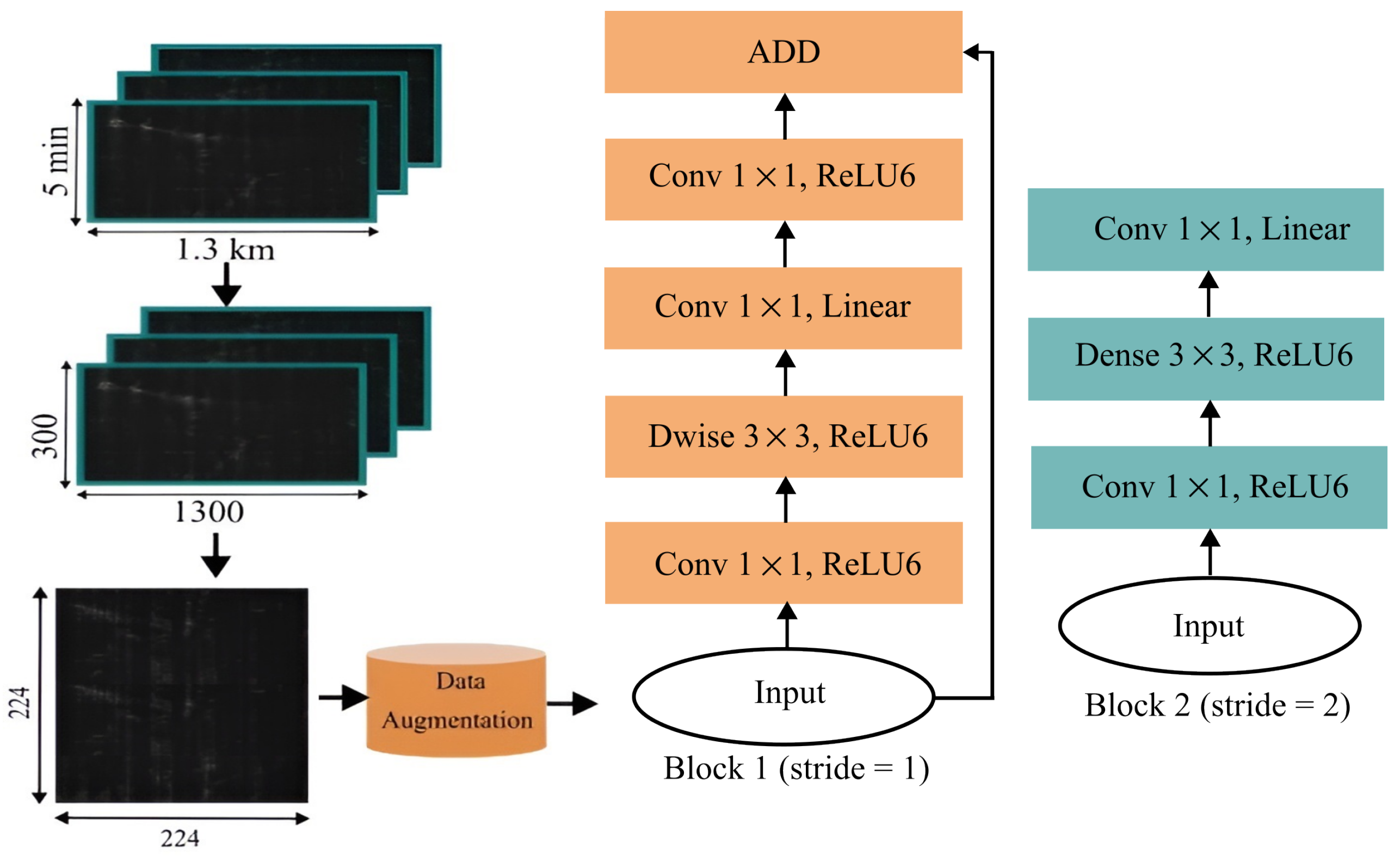
2.2. MobileNetV2 Architecture

MobileNet is a deep learning architecture known for its computational efficiency, making it suitable for resource-constrained environments such as mobile devices and embedded systems [33]. Its main features are depth-wise separable convolutional layers and inverted residuals. It is composed of an input layer, convolutional layers, and fully connected layers. This study demonstrates the application of MobileNetV2 to a multi-class image classification task, specifically focusing on $\varphi$-OTDR waterfall image classification. The MobileNetV2 architecture employed in this study is depicted in Figure 4, showing the respective dimensions in each layer of the CNN. Images are presented to the MobileNetV2 with dimensions of $224\times 224$ in RGB color mode, as required by the model. The total data are divided into training and validation sets, with a validation split of 0.2 for vehicle counting and 0.15 for average speed estimation. MobileNetV2 is pre-trained using ImageNet weights. After the MobileNetV2 layers, a global average pooling layer is set, followed by a fully connected (FC) layer with one-hundred-forty neurons, a dropout rate of 0.1, and finally an output layer with six neurons for vehicle counting estimation and fourteen neurons for speed estimation (as for ViT). L1 and L2 regularization are also applied to the dense layer in the classification head, with L1 = 0.001 and L2 = 0.0005. The Softmax activation function is used. A learning rate scheduler is set with an initial value of $lr=0.001$, decaying by 50% every 10 epochs. The categorical cross-entropy loss function is used. The model is trained for 100 epochs, as in the previous case. The MobileNetV2 model has approximately 2 × ${10}^6$ parameters.

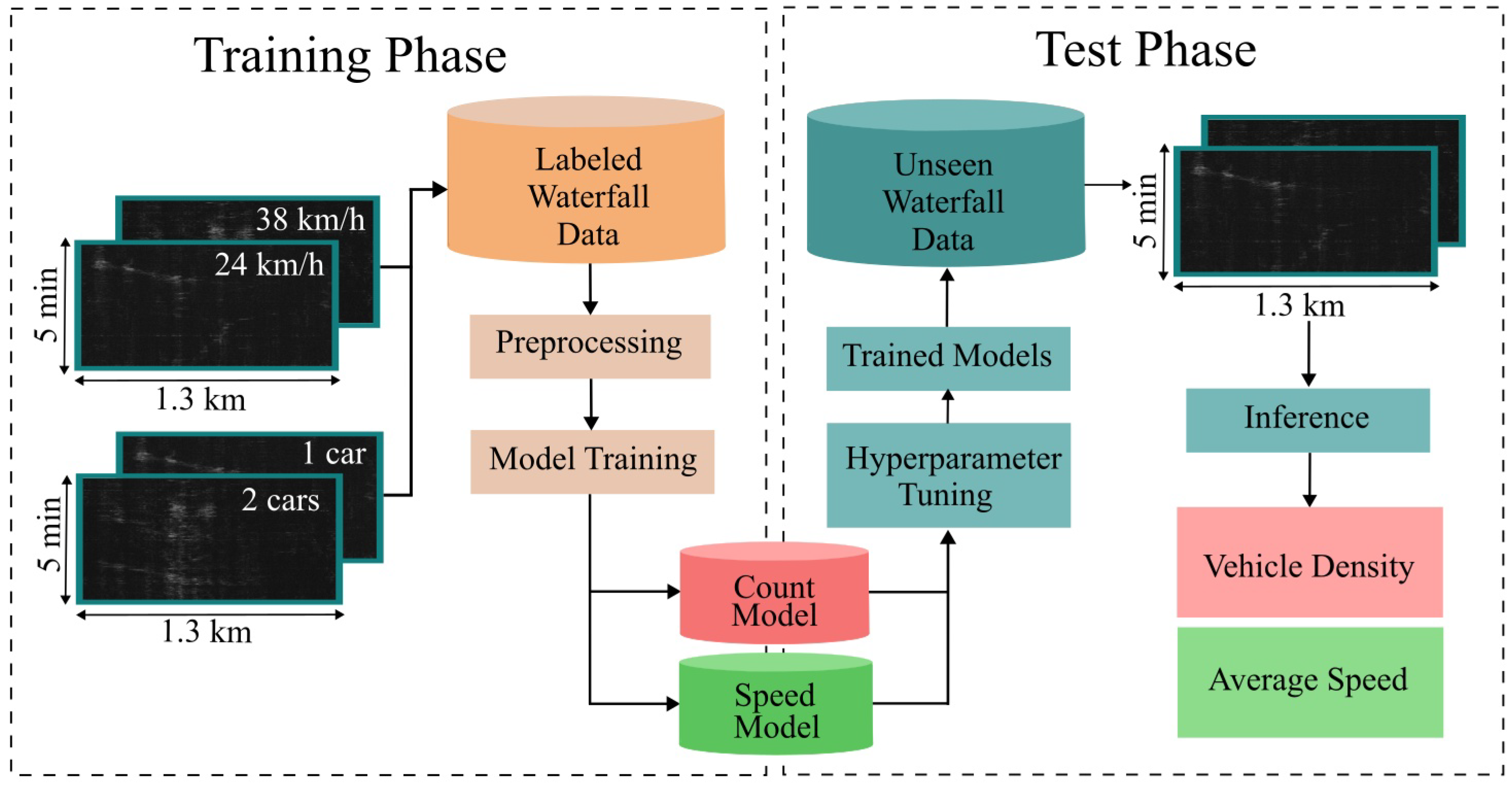
2.3. Preparation, Training, and Performance Evaluation

2.3.1. Image Preprocessing and Data Augmentation

As the patterns to be recognized do not occupy wide areas on images, the average value of pixels lies around the noise level. Therefore, we apply conventional min–max normalization as a preprocessing step. Data augmentation techniques are evaluated for both DL models. The augmentation techniques tested include random translation, zoom, contrast, Gaussian blur, flip, erosion, and the addition of Gaussian noise. Rescaling from [0–255] to [0, 1] is applied before submitting the images to the ViT and CNN to prevent fluctuations during training and expedite convergence. The augmentation parameters are empirically chosen during hyperparameter optimization. Also, the batch size of 8 is empirically determined. The impact of augmentation is empirically evaluated by assessing the performance metrics after training.

2.3.2. Model Training and Performance Evaluation

A summary of the training process is depicted in Figure 5. The dataset is initially divided into training and validation sets inside the stratified k-fold cross-validation loop. We use stratified k-fold to address class imbalances and have statistically represented classes in training and validation sets. The train–validation split is set to 0.2 for vehicle counting and approximately 0.15 for average speed estimation ($k=5$ and $k=7$ for k-fold cross-validation for car counting and speed estimation, respectively). The preprocessing layers are empirically tested, and the performance of the validation set is assessed. The model is first trained for 25 epochs for hyperparameter optimization, including a number of FC layers, FC neurons, and loss functions. The evaluated metrics cover the area under the receiver operating characteristic curve (AUC-ROC, adapted for multi-class classification), accuracy, validation loss, F1 score, precision, root mean squared error (RMSE), and recall. Following testing with multiple metrics, accuracy was selected as the primary evaluation criterion, yielding the best performance on previously unseen data. The other metrics are only used for further analysis. After training and validation, inference is applied over unseen data to assess the traffic behavior during arbitrary days.

For the entire training and performance assessment, we use the Keras library and NVIDIA GeForce GTX 1660 graphic processing unit (GPU). The GPU driver 556.12 is used, with Python 3.10.13, Tensorflow 2.10.1, CUDA 12.5, and cudnn 8.1.0.77 versions.

Table 1. Computational complexity of DL models.

Model	Parameters	MAC (G)	RAM (MB)
MNet Car Count	2,388,614	2.40	869.18
ViT Car Count	86,488,454	1.61	1647.69
MNet Speed	2,405,186	2.40	869.25
ViT Speed	86,498,882	1.61	1647.73

shows a comparison of the MobileNetV2 and ViT models for both classification tasks during training regarding the number of parameters, multiply–accumulate (MAC) operations, and total memory occupation. The ViT requires a substantially higher number of parameters (40-fold). However, despite having fewer parameters, MobileNetV2 requires more MAC operations due to the spatial nature of the convolution. In terms of random access memory, MobileNetV2 requires half the capacity. The results indicate equivalent computational complexity for both models.

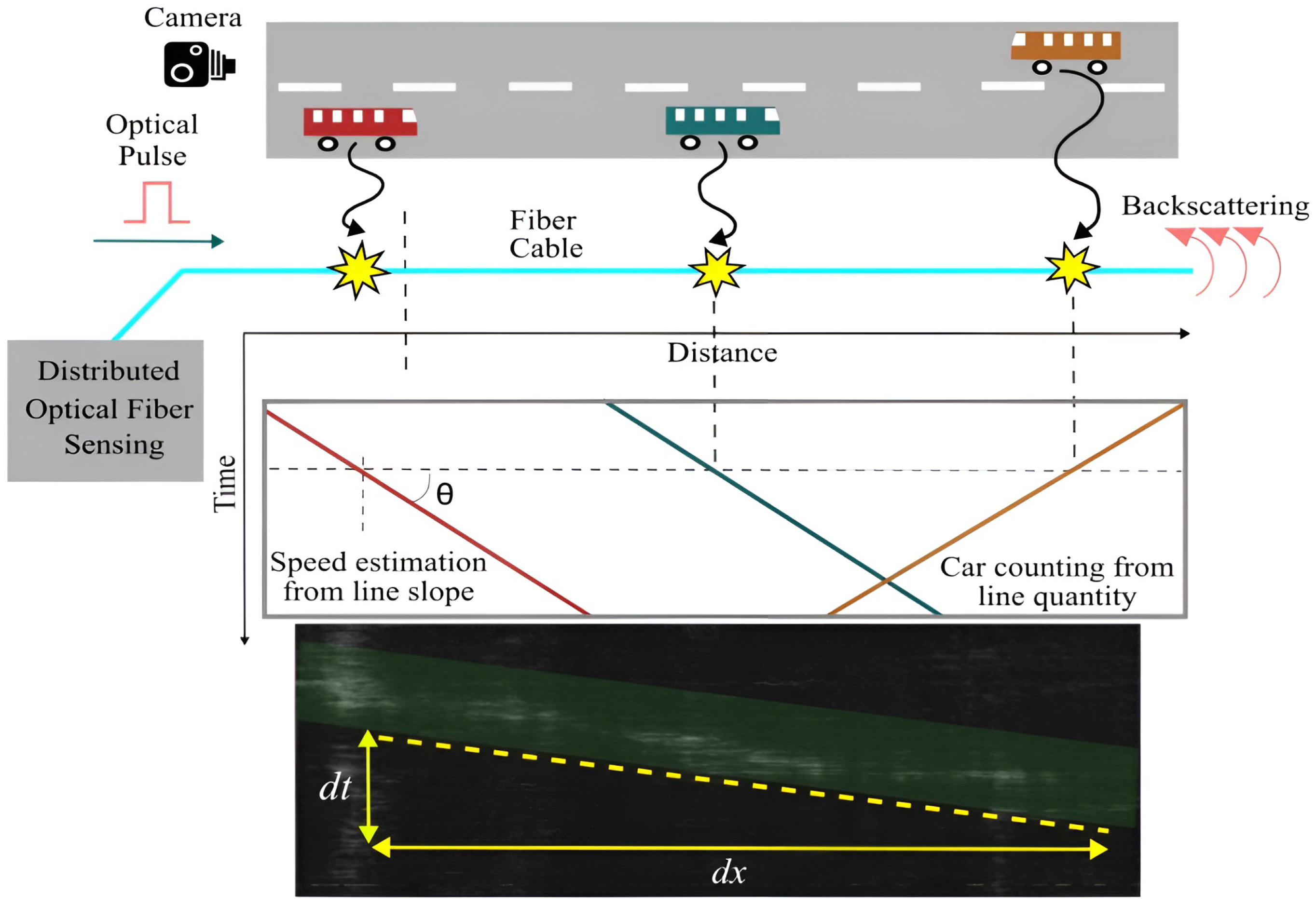
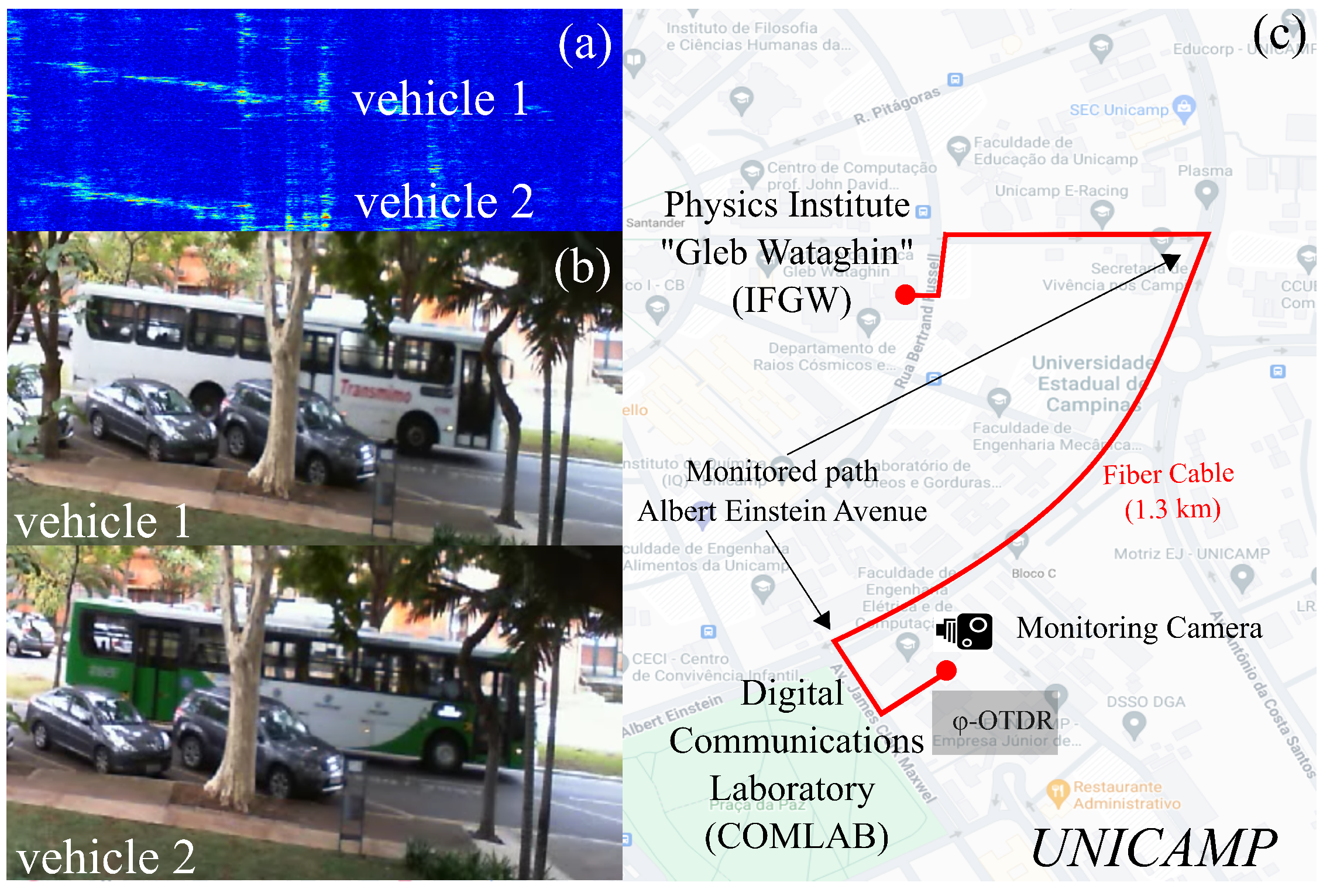
3. Experimental Setup

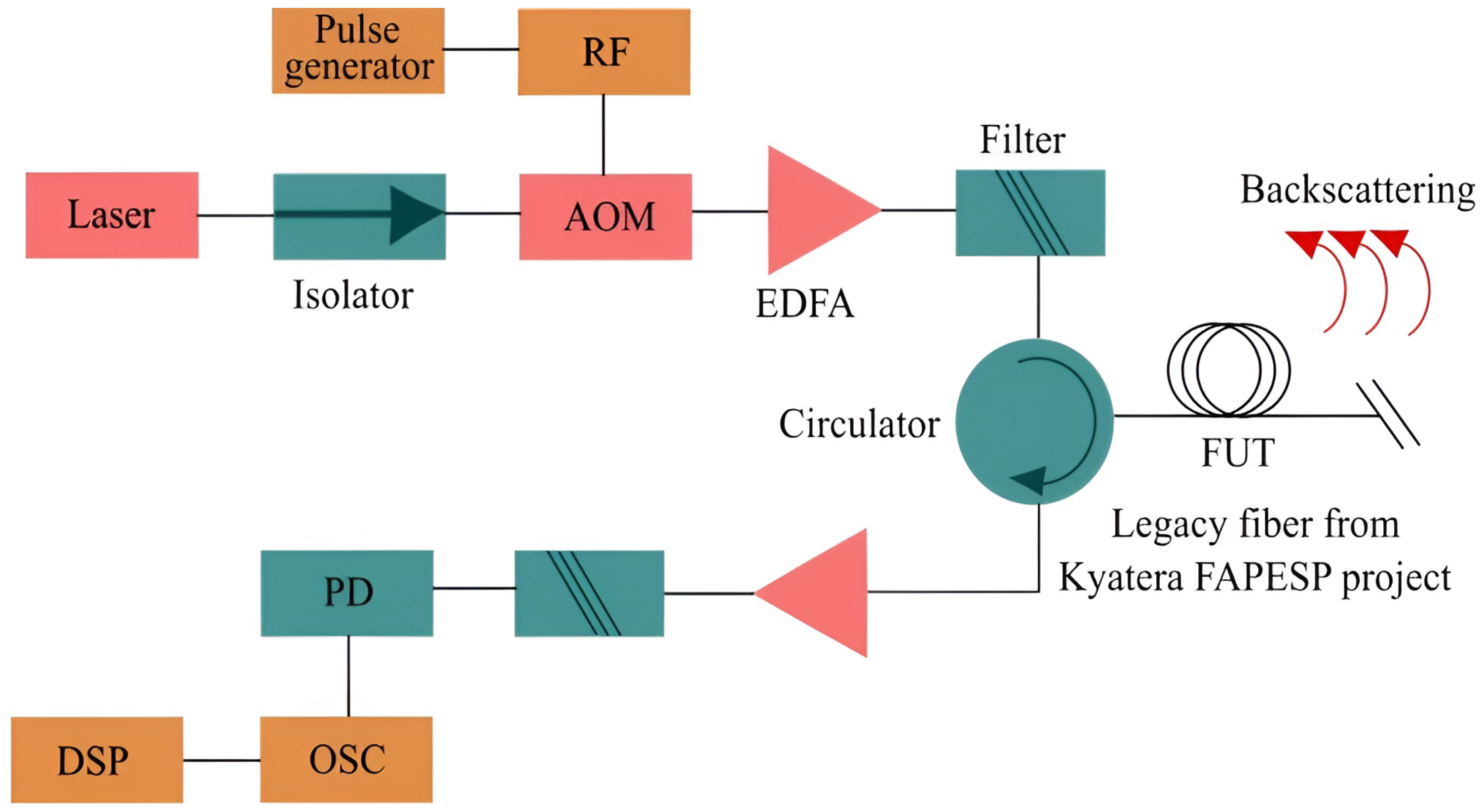
3.1. $\varphi$-OTDR Setup

The field trial is based on a 1.3 km buried legacy fiber cable connecting the electrical engineering and physics departments. The cables are buried approximately 1 to 1.5 m beneath the sidewalk, displaced about 1 m away from the street, which helps to filter out background noise. The direct-detection-based $\varphi$-OTDR setup is depicted in Figure 6. A pulse generator (81110A, Agilent, Santa Clara, CA, USA) producing 500 ns pulses with a 100 ms period is connected to a vector signal generator (RF, Agilent E4438C), feeding an acousto-optic modulator (AOM, NEOS FOAOM 26055-1-1.55, 55 MHz). The modulator takes as input a laser (Laser, Redfern Integrated Optics RIO0184-3-01-4-C9) with a small linewidth [36] operating at a 1551.72 nm wavelength and 5 dBm power. An isolator is used after the laser to prevent spurious reflections. The pulsed signal is then amplified by a two-stage erbium-doped fiber amplifier (EDFA, Padtec LOAC211GAH), followed by a 0.1 nm band pass filter to decrease amplified spontaneous emission (ASE) noise. The amplified optical signal is launched into the fiber under test (FUT), preceded by a 3.7 km spool, via a circulator. The Rayleigh backscattering is collected by the circulator, amplified, and filtered again to decrease ASE noise. The filtered signal is sent to a photoreceiver (PD, Lasertron QDFB 005-103), followed by an oscilloscope (OSC, Agilent MSO9404A) and a Python-built DSP acquisition system. The traces are then processed to obtain images representing variations over time and distance. $\varphi$-OTDR traces are concatenated into 5 min timestamped data.

Figure 7 presents examples of generated images, referred to as waterfall diagrams, over time and distance under various speed situations. The images are generated in a controlled environment by driving a heavy car on the monitored street.

Automatic collection is implemented in Python. The scope is set up within a segmented collection configuration, so the collected traces are concatenated in a matrix A with elements $a_{mn}$, where m represents time and n represents distance. Waterfall diagrams are generated in these arrays. Vehicle data appear as stripes formed by high-intensity pixels after the subtraction of consecutive lines in A. For the 1.3 km fiber, 26,000 samples are collected for one pulse. Due to the 500 ns pulse width, the spatial resolution is 50 m. This limitation is imposed by the AOM rise time, which is approximately 250 ns. Although the 50 m spatial resolution poses challenges in differentiating closely spaced vehicles, for most applications, e.g., traffic flow monitoring and traffic interruption detection, detecting each vehicle independently is not the primary concern but the collective behavior of a set of vehicles in an observed time frame. The collection period is empirically chosen based on average vibration frequencies found in vehicular movements, which are around 5–10 Hz. Each collection represents 5 min, corresponding to 3000 traces with 26,000 points each, which are stacked in the form of a matrix. The 3000 × 26,000 matrix is transferred in byte format to filter noise and speed up collection. Consecutive lines are subtracted to produce a differential 2999 × 26,000 matrix. Min–max normalization is applied as a preprocessing step. This differential matrix is transformed into a PNG image and resized to a 300 × 1300 format.

3.2. Camera Setup

A camera is installed on the monitored road. The camera data capture script runs synchronously with the $\varphi$-OTDR capture script. Therefore, for every collected $\varphi$-OTDR trace, a 5 min camera video is collected and stored. The two recording systems have a ping delay in the order of milliseconds, which is negligible considering the 5 min recording time and the vehicle transit times. The codes run concomitantly and save $\varphi$-OTDR data and camera videos with the same label. Due to power limitations at the laser and the photoreceiver maximum input power to avoid saturation, only heavy vehicles can be detected by using the collected images (vans, buses, and trucks). To avoid biases and allow subsequent experiments with preprocessing techniques, no prior preprocessing is carried out over the $\varphi$-OTDR raw data and over camera recordings. Raw data arrays are transformed into images and an image dataset is built. To assess image features and establish a ground truth, we apply the YOLOv8 [34,37] algorithm with tracking to detect buses and trucks in 5 min videos synchronized with the $\varphi$-OTDR traces. YOLOv8 is a computer vision model that classifies objects along video frames. Depending on video quality, YOLOv8 accurately detects people, vehicles, trucks, and buses. The deployed YOLOv8 architecture is used for bus and truck tracking, processing at 15 FPS and assigning stable identifiers (IDs) across frames. This method accurately counts and determines the speed of heavy vehicles by correlating unique IDs with the actual distance covered by object boxes in video frames. Diagonal linear features are correlated with unique YOLOv8-tracked IDs, working as a ground truth. Two labels are generated with YOLOv8: vehicle car count in a 5 min time frame and average speed. Vehicle counts are extracted by counting tracking IDs from YOLOv8. Average speed is obtained by calculating it from the displacement of object boxes detected by the YOLOv8.

3.3. Dataset

The images in the dataset are labeled with car density and average speed information. Due to the scarcity of more than 5 heavy vehicles in a 5 min time frame, a class for 5 or more vehicles was created, so six classes are considered for car counting. The quantity of samples per class used for car counting is displayed in

Table 2. Dataset classes for car count (a) and speed estimation (b).

(a) Car Count		(b) Average Speed
Class	Samples	Class	Samples
0	482	0–4.99 km/h	251
1	479	5–9.99 km/h	1
2	182	10–14.99 km/h	3
3	35	15–19.99 km/h	9
4	9	20–24.99 km/h	36
5+	11	25–29.99 km/h	76
–	–	30–34.99 km/h	171
–	–	35–39.99 km/h	162
–	–	40–44.99 km/h	137
–	–	45–49.99 km/h	49
–	–	50–54.99 km/h	51
–	–	55–59.99 km/h	10
–	–	60–64.99 km/h	1
–	–	65–70 km/h	6

a. For speed estimation, the images are divided into 14 classes, each representing a 5 km/h speed bin. As very high speeds are not allowed inside the university campus, only speeds up to 70 km/h are considered. To address class imbalance and avoid classification bias, the most populated class (i.e., “0”) is limited to 251 images. The quantity of samples per class for speed estimation is shown in Table 2b. Vehicles whose speeds are in the range 5–20 km/h and above 55 km/h are uncommon in the monitored street. Data augmentation techniques are used to deal with this imbalance. For car counting, random contrast, zooming, translation, brightness, blurring, and additive noise are chosen as augmentation techniques. For average speed estimation, random contrast, brightness, blurring, and additive noise are set for data augmentation.

The image filenames contain the vehicle quantity and average speed. A sample filename is “3_28.12015_1300m_300s_500ns_per100ms_byte_Feb-23-2024_08_49_26”.

Table 3. Parameters in dataset filenames.

Parameter	Example in Filename	Unit
Vehicle quantity	3	vehicles
Average speed	28.12015	[km/h]
Fiber length	1300 m	[m]
Collection period	300 s	[s]
Pulse width	500 ns	[ns]
Pulse period	100 ms	[ms]
Collection mode	byte	string
Timestamp	Feb-23-2024_08_49_26	string

explains the parameters presented in the sample filename. The first parameter is the number of vehicles in the image. In the example, “3” indicates that YOLOv8 detected three heavy vehicles in the recorded time frame. The average speed, calculated from the box displacement in the YOLOv8 tracking function, is represented with five decimals in km/h. The fiber length is constant for the entire dataset, 1300 m. The collection period is also constant, 5 min or 300 s, for all images. The pulse width is constant at 500 ns. The collection period is constant at 100 ms. Data collection is carried out in BYTE mode.

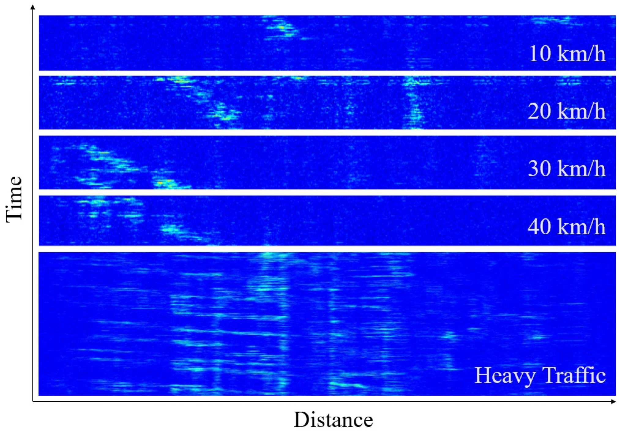
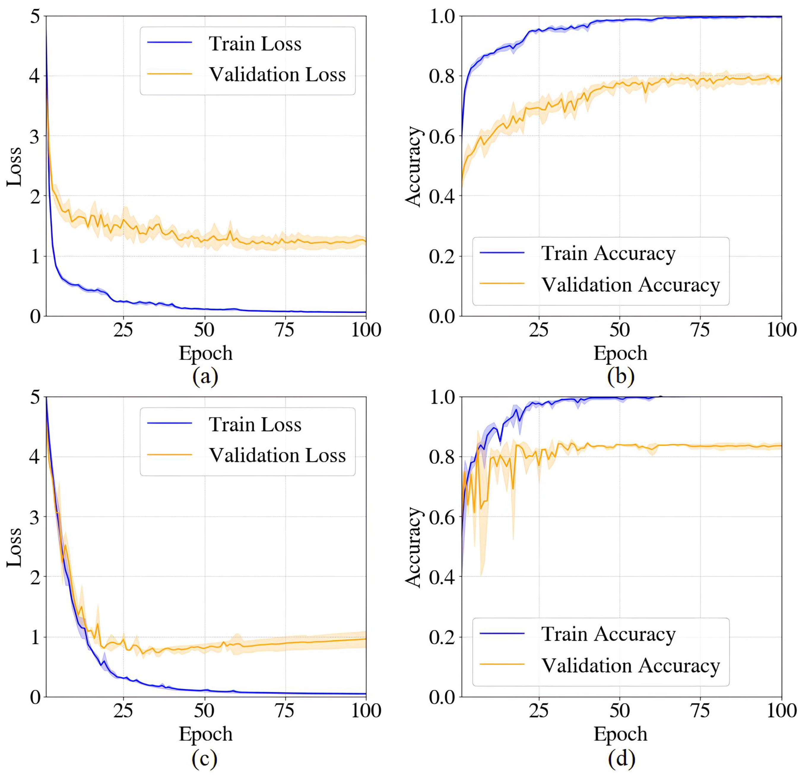
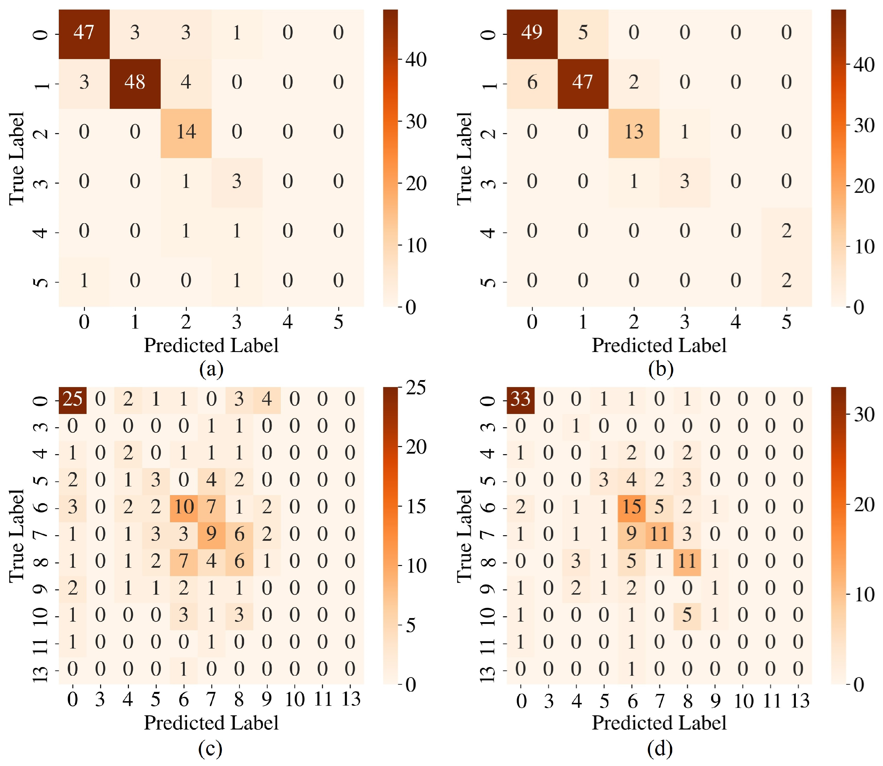
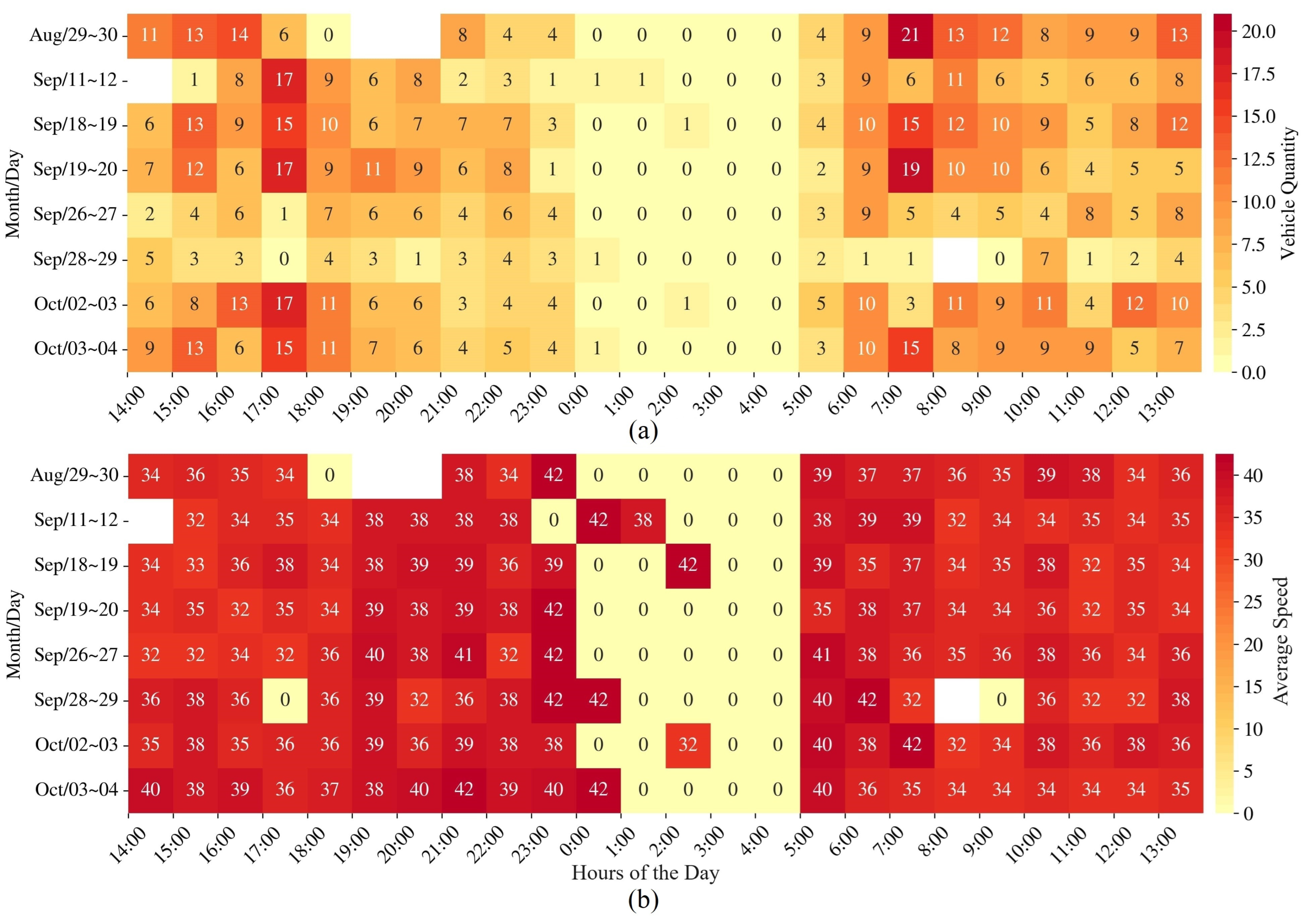
4. Results and Discussion

Figure 8 presents the training and validation loss and accuracy for MobileNetV2 (Figure 8a,b) and ViT (Figure 8c,d) for vehicle counting. The curves present the average loss and accuracy for $k=5$, along with the standard deviation across the folds. ViT reaches a smaller validation loss and a higher validation accuracy. Figure 9 shows the training and validation loss and accuracy for MobileNetV2 (Figure 9a,b) and ViT (Figure 9c,d) for average speed estimation. A value of $k=7$ is used for cross-validation for both speed estimation models. Again, ViT shows reduced validation loss and improved validation accuracy. The figure also emphasizes the superiority of ViT over MobileNetV2 in parameter estimation tasks.

Figure 10 depicts the confusion matrices for car counting (Figure 10a,b) and speed estimation (Figure 10c,d) for the MobileNetV2 and ViT models. In the confusion matrices, the true labels from YOLOv8-based detection are placed on the y-axis, while the predicted labels from DL models are shown on the x-axis. The test set for car counting comprises 131 unseen images. Over this test set, the MobileNetV2 model reaches an accuracy of 0.85, while ViT performs slightly better, with an accuracy of 0.87. For speed estimation, MobileNetV2 attains an accuracy of 0.36, compared to 0.50 for ViT on the validation set. Due to highly imbalanced classes in the speed estimation task, no test set was used. Instead, the confusion matrices are generated based on the validation set for the best fold ($k=7$).

Classes 1, 2, and 12 of the speed dataset are excluded from the cross-validation loop as they lack sufficient samples for training and validation. These classes correspond to speed ranges of 5–9.99 km/h, 10–14.99 km/h, and 60–64.99 km/h, respectively. As the field trial takes place on a campus street, classes with fewer heavy vehicles are dominant. This characteristic should also be commonly encountered in smart cities with local traffic. As expected, ViT takes more time for inference (15.86 ms per image) than MobileNetV2 (2.19 ms per image). These numbers are acceptable for real-time applications as the vehicle transit time is in the order of seconds and the total collection time is in the minute scale. Estimating outlier speeds is a challenge for both algorithms due to the imbalanced dataset. This limitation should also be encountered in practice, following the particularities of each monitored road.

Figure 11 illustrates the application of the investigated DL algorithms in a practical scenario of road monitoring. The figure presents the ViT performance for eight days of testing with unseen data, monitored continuously over a 24-h period. The white squares in the figure represent hours when the system was offline due to technical issues. The figure demonstrates the system’s ability to estimate traffic using $\varphi$-OTDR traces, detecting heavy traffic during peak hours and low vehicle counts during the night. Analyzing the distinctive features of specific days reveals interesting patterns. The rise in traffic on 29–30 August can be traced back to a noteworthy campus event, while the dip in traffic on 26–27 September coincides with occurrences impacting campus traffic. The analysis underscores the potential of $\varphi$-OTDR-based DFOS systems for traffic control in a smart community context.

5. Conclusions

Regarding an expanded vision of 6G as a wired/wireless integrated joint communication and sensing platform, we propose and evaluate advanced machine-learning-based image processing techniques for traffic monitoring in smart cities using a low-cost phase-sensitive OTDR. The investigated algorithms are assessed using an experimental low-cost DFOS system installed over a fiber-optic cable buried within a university campus. Data are simultaneously collected by the $\varphi$-OTDR setup and a dedicated camera whose videos are processed by the YOLOv8 algorithm, defined as ground truth. The collected data are labeled with vehicle density and average speed and fed to MobileNetV2 and ViT models for training. The inference drawn from unseen data provides a robust estimation of traffic behavior. The ViT model exhibits increased performance compared with the MobileNetV2 model when applied to both vehicle counting and average speed estimation. As a case study, the ViT model is applied to monitor the traffic for eight entire days, revealing interesting patterns and grasping the actual traffic profile on the campus. While the ViT necessitates a significantly larger number of parameters, its complexity is similar to that of a CNN when considering multiply–accumulate operations and random access memory usage. Finally, the dataset used to generate this work is made public for benchmarking.

References

1. Letaief, K.B.; Chen, W.; Shi, Y.; Zhang, J.; Zhang, Y.J.A. The Roadmap to 6G: AI Empowered Wireless Networks. IEEE Commun. Mag. 2019, 57, 84–90. [Google Scholar] [CrossRef]
2. Wymeersch, H.; Shrestha, D.; de Lima, C.M.; Yajnanarayana, V.; Richerzhagen, B.; Keskin, M.F.; Schindhelm, K.; Ramirez, A.; Wolfgang, A.; de Guzman, M.F.; et al. Integration of Communication and Sensing in 6G: A Joint Industrial and Academic Perspective. In Proceedings of the 2021 IEEE 32nd Annual International Symposium on Personal, Indoor and Mobile Radio Communications (PIMRC), Helsinki, Finland, 13–16 September 2021; pp. 1–7. [Google Scholar] [CrossRef]
3. Wild, T.; Braun, V.; Viswanathan, H. Joint Design of Communication and Sensing for Beyond 5G and 6G Systems. IEEE Access 2021, 9, 30845–30857. [Google Scholar] [CrossRef]
4. Liu, F.; Cui, Y.; Masouros, C.; Xu, J.; Han, T.X.; Eldar, Y.C.; Buzzi, S. Integrated Sensing and Communications: Toward Dual-Functional Wireless Networks for 6G and Beyond. IEEE J. Sel. Areas Commun. 2022, 40, 1728–1767. [Google Scholar] [CrossRef]
5. Boffi, P.; Ferrario, M.; Luch, I.D.; Rizzelli, G.; Gaudino, R. Optical sensing in urban areas by deployed telecommunication fiber networks. In Proceedings of the 2022 International Conference on Optical Network Design and Modeling (ONDM), Warsaw, Poland, 16–19 May 2022; pp. 1–5. [Google Scholar] [CrossRef]
6. Mello, D.A.A.; Mayer, K.S.; Escallón-Portilla, A.F.; Arantes, D.S.; Pinto, R.P.; Rothenberg, C.E. When Digital Twins Meet Optical Networks Operations. In Proceedings of the 2023 Optical Fiber Communications Conference and Exhibition (OFC), San Diego, CA, USA, 5–9 March 2023; pp. 1–3. [Google Scholar] [CrossRef]
7. Aono, Y.; Ip, E.; Ji, P. More than Communications: Environment Monitoring Using Existing Optical Fiber Network Infrastructure. In Proceedings of the Optical Fiber Communication Conference (OFC) 2020, San Diego, CA, USA, 8–12 March 2020; Optica Publishing Group: Washington, DC, USA, 2020; pp. 1–3. [Google Scholar] [CrossRef]
8. Xia, T.J.; Wellbrock, G.A.; Huang, M.F.; Salemi, M.; Chen, Y.; Wang, T.; Aono, Y. First Proof That Geographic Location on Deployed Fiber Cable Can Be Determined by Using OTDR Distance Based on Distributed Fiber Optical Sensing Technology. In Proceedings of the Optical Fiber Communication Conference (OFC) 2020, San Diego, CA, USA, 8–12 March 2020; Optica Publishing Group: Washington, DC, USA, 2020; pp. 1–3. [Google Scholar] [CrossRef]
9. Tucker, R.; Ruffini, M.; Valcarenghi, L.; Campelo, D.R.; Simeonidou, D.; Du, L.; Marinescu, M.C.; Middleton, C.; Yin, S.; Forde, T.; et al. Connected OFCity: Technology innovations for a smart city project [Invited]. J. Opt. Commun. Netw. 2017, 9, A245–A255. [Google Scholar] [CrossRef]
10. Rao, Y.; Wang, Z.; Wu, H.; Ran, Z.; Han, B. Recent advances in phase-sensitive optical time domain reflectometry (ϕ-OTDR). Photonic Sens. 2021, 11, 1–30. [Google Scholar] [CrossRef]
11. Hancke, G.P.; Silva, B.D.C.e.; Hancke, G.P., Jr. The Role of Advanced Sensing in Smart Cities. Sensors 2013, 13, 393–425. [Google Scholar] [CrossRef]
12. Jia, Z.; Campos, L.A.; Xu, M.; Zhang, H.; Gonzalez-Herraez, M.; Martins, H.F.; Zhan, Z. Experimental Coexistence Investigation of Distributed Acoustic Sensing and Coherent Communication Systems. In Proceedings of the 2021 Optical Fiber Communications Conference and Exhibition (OFC), San Francisco, CA, USA, 6–11 June 2021; pp. 1–3. [Google Scholar]
13. Juarez, J.; Maier, E.; Choi, K.N.; Taylor, H. Distributed fiber-optic intrusion sensor system. J. Light. Technol. 2005, 23, 2081–2087. [Google Scholar] [CrossRef]
14. Ren, L.; Jiang, T.; Jia, Z.-g.; Li, D.-s.; Yuan, C.-l.; Li, H.-n. Pipeline corrosion and leakage monitoring based on the distributed optical fiber sensing technology. Measurement 2018, 122, 57–65. [Google Scholar] [CrossRef]
15. Fernández-Ruiz, M.R.; Soto, M.A.; Williams, E.F.; Martin-Lopez, S.; Zhan, Z.; Gonzalez-Herraez, M.; Martins, H.F. Distributed acoustic sensing for seismic activity monitoring. APL Photonics 2020, 5, 030901. [Google Scholar] [CrossRef]
16. Pastor-Graells, J.; Martins, H.F.; Garcia-Ruiz, A.; Martin-Lopez, S.; Gonzalez-Herraez, M. Single-shot distributed temperature and strain tracking using direct detection phase-sensitive OTDR with chirped pulses. Opt. Express 2016, 24, 13121–13133. [Google Scholar] [CrossRef]
17. Tejedor, J.; Macias-Guarasa, J.; Martins, H.F.; Pastor-Graells, J.; Martín-López, S.; Guillén, P.C.; Pauw, G.D.; Smet, F.D.; Postvoll, W.; Ahlen, C.H.; et al. Real Field Deployment of a Smart Fiber-Optic Surveillance System for Pipeline Integrity Threat Detection: Architectural Issues and Blind Field Test Results. J. Light. Technol. 2018, 36, 1052–1062. [Google Scholar] [CrossRef]
18. Williams, E.F.; Fernández-Ruiz, M.R.; Magalhaes, R.; Vanthillo, R.; Zhan, Z.; González-Herráez, M.; Martins, H.F. Distributed sensing of microseisms and teleseisms with submarine dark fibers. Nat. Commun. 2019, 10, 5778. [Google Scholar] [CrossRef] [PubMed]
19. Peng, F.; Duan, N.; Rao, Y.J.; Li, J. Real-Time Position and Speed Monitoring of Trains Using Phase-Sensitive OTDR. IEEE Photonics Technol. Lett. 2014, 26, 2055–2057. [Google Scholar] [CrossRef]
20. Xia, T.J.; Wellbrock, G.A.; Huang, M.F.; Han, S.; Chen, Y.; Salemi, M.; Ji, P.N.; Wang, T.; Aono, Y. Field Trial of Abnormal Activity Detection and Threat Level Assessment with Fiber Optic Sensing for Telecom Infrastructure Protection. In Proceedings of the 2021 Optical Fiber Communications Conference and Exhibition (OFC), San Francisco, CA, USA, 6–11 June 2021; pp. 1–3. [Google Scholar]
21. Lu, X.; Soto, M.A.; Thomas, P.J.; Kolltveit, E. Evaluating Phase Errors in Phase-Sensitive Optical Time-Domain Reflectometry Based on I/Q Demodulation. J. Light. Technol. 2020, 38, 4133–4141. [Google Scholar] [CrossRef]
22. Adeel, M.; Shang, C.; Hu, D.; Wu, H.; Zhu, K.; Raza, A.; Lu, C. Impact-Based Feature Extraction Utilizing Differential Signals of Phase-Sensitive OTDR. J. Light. Technol. 2020, 38, 2539–2546. [Google Scholar] [CrossRef]
23. Uyar, F.; Onat, T.; Unal, C.; Kartaloglu, T.; Ozbay, E.; Ozdur, I. A direct detection fiber optic distributed acoustic sensor with a mean SNR of 7.3 dB at 102.7 km. IEEE Photonics J. 2019, 11, 1–8. [Google Scholar] [CrossRef]
24. Kandamali, D.F.; Cao, X.; Tian, M.; Jin, Z.; Dong, H.; Yu, K. Machine learning methods for identification and classification of events in ϕ-OTDR systems: A review. Appl. Opt. 2022, 61, 2975–2997. [Google Scholar] [CrossRef]
25. Huang, M.F.; Salemi, M.; Chen, Y.; Zhao, J.; Xia, T.J.; Wellbrock, G.A.; Huang, Y.K.; Milione, G.; Ip, E.; Ji, P.; et al. First Field Trial of Distributed Fiber Optical Sensing and High-Speed Communication Over an Operational Telecom Network. J. Light. Technol. 2020, 38, 75–81. [Google Scholar] [CrossRef]
26. Catalano, E.; Coscetta, A.; Cerri, E.; Cennamo, N.; Zeni, L.; Minardo, A. Automatic traffic monitoring by ϕ-OTDR data and Hough transform in a real-field environment. Appl. Opt. 2021, 60, 3579–3584. [Google Scholar] [CrossRef]
27. Narisetty, C.; Hino, T.; Huang, M.F.; Ueda, R.; Sakurai, H.; Tanaka, A.; Otani, T.; Ando, T. Overcoming Challenges of Distributed Fiber-Optic Sensing for Highway Traffic Monitoring. Transp. Res. Rec. 2021, 2675, 233–242. [Google Scholar] [CrossRef]
28. Wang, T.; Huang, M.F.; Han, S.; Narisetty, C. Employing Fiber Sensing and On-Premise AI Solutions for Cable Safety Protection over Telecom Infrastructure. In Proceedings of the 2022 Optical Fiber Communications Conference and Exhibition (OFC), San Diego, CA, USA, 6–10 March 2022; pp. 1–3. [Google Scholar]
29. Liu, S.; Yu, F.; Hong, R.; Xu, W.; Shao, L.; Wang, F. Advances in phase-sensitive optical time-domain reflectometry. Opto-Electron. Adv. 2022, 5, 200078-1. [Google Scholar] [CrossRef]
30. Bao, X.; Wang, Y. Recent Advancements in Rayleigh Scattering-Based Distributed Fiber Sensors. Adv. Devices Instrum. 2021, 2021, 8696571. [Google Scholar] [CrossRef]
31. Ip, E.; Fang, J.; Li, Y.; Wang, Q.; Huang, M.F.; Salemi, M.; Huang, Y.K. Distributed fiber sensor network using telecom cables as sensing media: Technology advancements and applications [Invited]. J. Opt. Commun. Netw. 2022, 14, A61–A68. [Google Scholar] [CrossRef]
32. Colares, R.A.; Conforti, E.; Rittner, L.; Mello, D.A. Field Trial of an ML-Assisted Phase-Sensitive OTDR for Traffic Monitoring in Smart Cities [invited]. In Proceedings of the 2024 24th International Conference on Transparent Optical Networks (ICTON), Bari, Italy, 14–18 July 2024; pp. 1–4. [Google Scholar] [CrossRef]
33. Sandler, M.; Howard, A.; Zhu, M.; Zhmoginov, A.; Chen, L.C. MobileNetV2: Inverted Residuals and Linear Bottlenecks. In Proceedings of the 2018 IEEE/CVF Conference on Computer Vision and Pattern Recognition, Salt Lake City, UT, USA, 18–22 June 2018; pp. 4510–4520. [Google Scholar] [CrossRef]
34. Colares, R.A.; Huancachoque, L.; Conforti, E.; Mello, D.A. Demonstration of ϕ-OTDR-based DFOS Assisted by YOLOv8 for Traffic Monitoring in Smart Cities. In Proceedings of the 2024 SBFoton International Optics and Photonics Conference (SBFoton IOPC), Salvador, Brazil, 11–13 November 2024; pp. 1–3. [Google Scholar]
35. Vaswani, A.; Shazeer, N.; Parmar, N.; Uszkoreit, J.; Jones, L.; Gomez, A.N.; Kaiser, L.; Polosukhin, I. Attention is all you need. In Proceedings of the 31st International Conference on Neural Information Processing Systems, NIPS’17, Red Hook, NY, USA, 4–9 December 2017; pp. 6000–6010. [Google Scholar]
36. Sutili, T.; Figueiredo, R.C.; Conforti, E. Laser Linewidth and Phase Noise Evaluation Using Heterodyne Offline Signal Processing. J. Light. Technol. 2016, 34, 4933–4940. [Google Scholar] [CrossRef]
37. Jocher, G.; Chaurasia, A.; Qiu, J. Ultralytics YOLOv8. 2023. Available online: https://docs.ultralytics.com/models/yolov8/ (accessed on 1 February 2024).
38. Colares, R.A.; Conforti, E.; Mello, D.A.A. Dataset Related to Paper “Fiber Sensing in the 6G Era: Vision Transformers for ϕ-OTDR-Based Road-Traffic Monitoring”. 2024. Available online: https://redu.unicamp.br/dataset.xhtml?persistentId=doi:10.25824/redu/VLHHAW (accessed on 1 February 2024).
Figure 1. Traffic monitoring scheme with ϕ -OTDR-based DFOS. Data are simultaneously collected from DFOS system and video camera. Concatenated ϕ -OTDR traces form images along time (dt) and distance (dx), allowing vehicle density counting and speed estimation through line slope.
Applsci 15 03170 g001
Figure 2. Waterfall traces corresponding to two vehicles (a). The respective video frames (b). Monitored fiber path on the university campus (c).
Applsci 15 03170 g002
Figure 3. Vision transformer architecture for traffic parameter estimation. The input image is split into patches, each patch is linearly projected and combined with positional embeddings, and then passed through a transformer encoder for car counting and speed estimation. MLP: multilayer perceptron. The 300 × 1300 input images are resized to 224 × 224 for further augmentation and patch creation.
Applsci 15 03170 g003
Figure 4. MobileNetV2 architecture. The arrows in the block diagram show how data flows through each inverted residual block. A skip connection (ADD) appears only in stride = 1 blocks, in which input and output dimensions match. Conv: convolutional layer; ReLU: rectifier unit; Dwise: depth-wise convolution.
Applsci 15 03170 g004
Figure 5. General process of DL model training for MobileNetV2 and ViT. Waterfall traces are labeled regarding car quantity and average speed, preprocessed, and submitted to DL models for vehicle density and average speed estimation. After hyperparameter tuning, inference is done over unseen images.
Applsci 15 03170 g005
Figure 6. Experimental setup of ϕ -OTDR-based DFOS. A narrow linewidth laser is pulsed by an AOM. The resulting signal is amplified by an EDFA, filtered, and launched into the optical fiber. The backscattering is collected by a circulator, amplified, filtered, photodetected, and recorded by the scope. RF: radiofrequency generator; AOM: acousto-optic modulator; EDFA: erbium-doped fiber amplifier; FUT: fiber under test; PD: photodetector; OSC: osciloscope; DSP: digital signal processing.
Applsci 15 03170 g006
Figure 7. Characterization of vehicle speeds around the campus avenue, showing four speeds: 10, 20, 30, and 40 km/h. Below, an example of waterfall diagram in a busy 5 min traffic frame.
Applsci 15 03170 g007
Figure 8. Train and validation loss and accuracy for car counting using MobileNetV2 (a,b) and vision transformer (c,d) using k = 5 for cross-validation.
Applsci 15 03170 g008
Figure 9. Train and validation loss and accuracy for speed estimation applying MobileNetV2 (a,b) and vision transformer (c,d) using k = 7 for cross-validation.
Applsci 15 03170 g009
Figure 10. Confusion matrices over unseen data for vehicle counting with MobileNetV2 (a) and ViT (b), and for speed estimation with MobileNetV2 (c) and ViT (d).
Applsci 15 03170 g010
Figure 11. Inference carried out by the ViT model applied to unseen ϕ -OTDR data for vehicle counting (a) and average speed (b) in 8 monitored days. The white squares represent technical events that prevented data collection.
Applsci 15 03170 g011