Abstract
Quantifying slope mechanical parameters as comprehensive indicators is crucial for predicting slope stability. The Mohr–Coulomb (M-C) criterion, a classical method for determining the relevant parameters of rock mass mechanics, effectively reflects the failure characteristics of rock masses in most types of slopes. Based on this, effective stress and shear strength from the M-C criterion are selected as key indicators, and a characteristic dataset is constructed by integrating these with other influencing factors of slope stability. The safety factor, calculated using the Bishop method within the framework of limit equilibrium analysis, serves as the output variable. Subsequently, a novel Black Kite Algorithm (BKA) was developed to enhance the prediction model of a multilevel perceptron neural network. The results demonstrate that the mean square error (RMSE) of the BKA-MLP model is merely 2.41%, significantly lower than that of alternative models. Additionally, the R2 value reaches approximately 95%, indicating a high level of interpretability. The SHAP-based interpretability analysis of the trained model highlights effective stress, shear strength, and slope angle as the three most sensitive features. Based on these findings, targeted landslide prevention measures were proposed, providing a new approach for slope stability analysis and disaster prevention.
1. Introduction
The issue of slope stability is not only pertinent to mining, geology, water conservancy, and other engineering disciplines but is also closely linked to environmental protection and urban planning. When an unstable slope experiences dynamic disturbances such as excavation, blasting, or earthquakes, it may result in catastrophic events like collapses and landslides, leading to casualties and significant property damage [1,2]. With the intensification of global climate change and the ongoing expansion of human activities, the frequency and scale of slope instability incidents are on the rise. This trend underscores the urgent need for accurate and efficient assessments of slope stability [3].
Traditional methods for analyzing slope stability—such as limit equilibrium analysis and finite element modeling—while providing valuable insights under certain conditions, often face limitations due to complex geological settings, nonlinear material behaviors, and external factors that are challenging to quantify (e.g., rainfall or seismic activity). These constraints can introduce uncertainties in practical applications. In recent years, machine learning has emerged as a powerful data-driven modeling tool that offers distinct advantages in addressing complex systems with high-dimensional data. This development paves new avenues for predicting slope stability effectively [4,5].
Jin Aibing et al. [6] built an SSA-SVM slope instability intelligent prediction model on the basis of establishing a database composed of 304 slope cases. Their results show that the SSA-SVM model performs well in various indicators and has certain competitiveness in slope classification prediction. Yan Xiaoming et al. [7] put forward a method to predict slope stability by using the Bayesian discriminant analysis theory. The model has good prediction performance and has certain practical engineering significance. Zhang Jiantao et al. [8] proposed a hybrid model of random forest optimized by the whale algorithm. Compared with the results of other models, it was found that all indexes of WOA-RF performed well, and the bulk density was found to be the most sensitive feature affecting slope stability. Nhat-Duc Hoanga et al. [9] combined the metaheuristic algorithm with machine learning, optimized LS-SVC with the firefly algorithm, and built a comprehensive prediction model. Experimental results showed that the classification accuracy of the new hybrid AI model was improved by about 4%.
The above scholars used different algorithms and machine learning methods to build slope stability prediction models, which provided certain positive effects for slope stability assessment, but there were certain limitations in slope stability identification. Instability and stability represent only two states of slope conditions, which fail to fully capture the complexity and dynamic nature of slope behavior [10]. Therefore, employing a regression model offers distinct advantages in predicting slope stability. The most widely utilized metric is the safety factor, as its value can precisely indicate the overall condition of the slope. Junlong Sun et al. [11] proposed a Stacking integrated learning model (BP-Stacking) based on Bayesian optimization. Their results found that the BOPStacking method can effectively improve the accuracy of predicting slope safety factors, and the mean square error is lower than that of a single model, and complex calculations are avoided. Zhang Sen et al. [12] used the sparrow search method to optimize the weight and bias parameters of the BP neural network, built an optimal model and tested it, and found that the predicted value of the optimized model was closer to the actual value. Wang Pengfei [13] used the combination of the GM model and RBF neural network to build a GM-RBF combined deformation prediction model for high cutting slope, and the results showed that the combined model was more feasible than the single model.
The regression prediction model combined with a neural network, a deep learning model, and various algorithms further improves the accuracy, but the complexity of the model also increases, making the model more difficult to explain. Xinzhi Zhou et al. [14] combined SHAP and XGBoost to explain landslide susceptibility assessment and found that peak rainfall intensity and altitude were the dominant factors affecting landslide occurrence. Chao Zhou et al. [15] proposed a PSO-SVM coupled model to predict landslide displacement and verified the prediction results by taking a typical step landslide in the Three Gorges Reservoir area as an example. Their results show that rainfall and water level are the dominant factors of landslide deformation. Zizheng Guo et al. [16] used the variational mode theory to decompose landslide step displacement, determined the mathematical relationship between random displacement and trigger factors through the GMO-BP model, and obtained the cumulative displacement prediction based on the time series model, which provided a certain reference for landslide displacement warning. In addition, some scholars have integrated the theory of rock mass mechanics to build a mixed model of rock mass mechanics and machine learning. Hou Kepeng et al. [17] built a multi-index system based on the Hawke Brown criterion, combined the sparrow search algorithm with a multilevel perceptual neural network, and verified the effectiveness of the model through practical cases. The results can be applied to most rock slopes.
Existing machine learning models, including Random Forest (RF), Long Short-Term Memory (LSTM), and Support Vector Machine (SVM), have shown promise in slope stability prediction but are subject to significant limitations. Specifically, RF is prone to overfitting when applied to high-dimensional datasets with limited samples, thereby diminishing its generalization capabilities in complex geological settings [8]. LSTM networks, designed primarily for sequential data and temporal dependencies, are not well-suited for static slope stability datasets. This mismatch leads to suboptimal accuracy and unnecessary computational overhead [18]. SVM faces challenges with large-scale datasets due to its reliance on quadratic programming, and its performance is highly sensitive to the choice of kernel function, introducing potential bias [19].
To address the limitations of traditional machine learning methods in data processing, feature selection, and interpretability, this study proposes a novel approach that integrates the comprehensive index of the M-C strength criterion with slope stability influencing factors. This integration effectively mitigates the complexity associated with feature selection. Furthermore, we employ BKA, a new metaheuristic intelligent algorithm, to optimize the primary structural parameters of the multilevel perceptron neural network, thereby enhancing the robustness and generalization capabilities of the model. The optimal model is interpreted using the SHAP method, revealing its physical significance in predictions and making the model’s decision-making process more transparent. The findings of this research provide valuable guidance for the development of slope stability control measures and hold significant practical engineering implications.
2. M-C Criterion and BKA-MLP Model Principle
2.1. M-C Principle
The M-C criterion [20] is one of the strength criteria widely used in geotechnical engineering to describe the shear strength characteristics of materials under stress conditions. The M-C criterion assumes that a material’s failure surface adheres to the maximum shear stress criterion—failure occurs when the shear stress at a point equals the material’s shear strength [21]. The M-C criterion is applicable to most rock and soil materials. Because of its clear concept, easy parameter acquisition, and simple calculation, the M-C criterion has been widely used in slope stability analysis, foundation engineering design, and stability evaluation of rock and soil structures. The M-C criterion expression is as follows:
where τ represents the shear strength, c is the cohesion force, σ′ is the effective stress, and φ is the internal friction angle. The effective stress can be calculated as follows:
where γ is the bulk density of rock mass, H is the height of the slope, ω is the bulk density of water, and z is the depth of groundwater level.
Among the above parameters, the cohesion force c reflects the bonding force between particles inside the material, while the internal friction angle φ describes the friction characteristics between particles, and c and φ can be measured by tests. Slope bulk density γ and slope height H can be measured directly on site; ω is a constant, 9.8 kN/m3 under standard conditions; z represents the information of water and rock mass strength of slope rock mass, which is difficult to measure on site and is affected by the specific conditions of the slope. Therefore, in this study, the z value under different conditions is calculated by the empirical formula method [22] combined with engineering practice and existing research [23], which is expressed as follows:
Both a and b are empirical parameters, and their values range from 0 to 20. To ensure the accuracy of the calculation results, the values of a and b are processed in segments [24].
In slope stability analysis, in recent years, the Hoek–Brown criterion is applied to slope types with obvious nonlinear characteristics, the Drucker–Prager criterion is applied to plastic slope, and the modified Cam-clay model has been more applicable to saturated soft clay slopes. However, when the traditional rock and soil mechanics theory and machine learning model are coupled to predict slope stability, the above strength theories have a certain one-sidedness, but the M-C strength criterion can capture the basic characteristics of materials well, and the use of the M-C strength criterion can often make the prediction model have a broader application space.
2.2. BKA Algorithm
BKA is a new metaheuristic optimization algorithm inspired by the predation behavior of kite hawks (black kites) in nature [25]. The design concept of the BKA algorithm is based on the behavior characteristics of kite hawks that hover in the air, locate targets, and hunt together. In the BKA, each candidate solution is treated as a member of a group of kite hawks who search by mimicking their flight patterns. Compared with other traditional optimization algorithms, the BKA algorithm maintains the dynamic balance of exploration and development mechanism on the basis of powerful global search ability. It has a relatively simple parameter setting, strong adaptability and stability, and a fast convergence rate of the BKA algorithm, which are certain advantages in slope stability prediction applications. The algorithm mainly defines three behavior patterns to guide the search process.
- Exploration Phase
This stage simulates the behavior of kite hawks searching for prey in a wide airspace. The algorithm increases the diversity of solutions by moving randomly, ensuring that the search space can be covered as large as possible in the search for potential high-quality solutions. First, the position Xi(t) of a group of kite hawks should be randomly initialized in the solution space, the mathematical expression is shown in the formula, and then the kite hawks search for potential food sources through random walks; the process is described as follows [26]:
where i = 1, 2, …; t is the number of iterations; L and U are the lower and upper limits of the variable, respectively, and rand is a random number between [0, 1].
where Xgb(t) is the best position of the current iteration; and α and β are the parameters controlling the exploration intensity. Usually set α = 2, is usually randomly selected from the uniform distribution U(0, 2π).
- 2.
- Exploitation Phase
After finding a promising area, the kite hawk will focus on a detailed search of the area in order to find the best prey, updating the rules as follows [27]:
where γ and δ are the parameters controlling the development degree; γ is usually set to 2; and δ is usually randomly selected from the uniform distribution U(0, 2π).
- 3.
- Social Learning Mechanism
There is an exchange of information between kite hawks, and they learn and adjust their strategies by observing the behavior of their peers. The social learning mechanism can be expressed by the following formula [28]:
where η is the learning rate used to adjust the learning speed.
2.3. MLP
MLP [29] is the artificial neural network input layer, a hidden layer, and the output layer. The layer contains multiple neurons; each neuron converts weighted input into output through an activation function. The basic structure is shown in Figure 1.
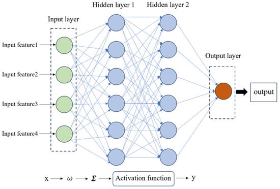
Figure 1.
MLP neural network structure.
In order to increase the computational efficiency of the model and reduce the risk of overfitting, a single hidden layer MLP network structure was adopted in this study. The number of neurons in the input layer is the number of input features set to m, the number of neurons in the hidden layer is set to n, and the number of neurons in the output layer is 1. In the forward propagation process, the output feature vector x ∈ Rm is passed to the hidden layer through the input layer, and the calculation is as follows [30]:
where z(1) represents the linear combination result of input and output to the hidden layer; , is the weight matrix from the input layer to the hidden layer; and b(1) is the bias vector of the hidden layer.
The calculation process from the hidden layer to the output layer is as follows [31]:
where represents the linear combination result from the hidden layer to the output layer; , is the weight matrix from the hidden layer to the output layer; is the hidden layer output; and is the output layer offset.
Activation functions introduce nonlinear properties, which enable neural network models to learn to represent complex nonlinear relationships. In the whole process, from the input feature to the hidden layer and then to the output layer, the activation function outputs the output of each process through nonlinear mapping. The main types of activation functions are as follows [32]:
The MLP model constantly adjusts and updates the connection weights and thresholds between neurons during training. The mean square error (MSE) is used as a fitness function to continuously optimize and find the minimum value to iteratively update the model during running, as shown [33] in Equation (13):
where represents the true value of sample i; represents the predicted value of sample i; n is the number of samples.
3. Database Establishment and Analysis
3.1. Feature Parameter Selection
Slope stability is a complex problem with multisystem, nonlinear, and multifactor influences. The multi-index system is based on the M-C strength criterion, and the BKA-MLP model is adopted to predict the safety factor of slope stability. The selected characteristic parameters should not only accurately reflect the failure characteristics of slope deformation and displacement characteristics but also cover the common characteristics of most slopes as comprehensively as possible. At the same time, the real conditions of the slope cannot be ignored [34]. Considering the influencing factors of slope stability and landslide mechanism, six influencing factors, namely two parameters of the M-C strength criterion (shear strength τ and effective stress σ′, kPa), the bulk density of slope rock mass (γ, kN/m3), slope geometry parameters (slope height H (m) and slope inclination α(°)), and pore ratio ru, are selected as the feature inputs of the prediction model. They are represented by X1 to X6. Compared with the traditional features of cohesion and internal friction angle, the use of shear strength and effective stress as features has more direct physical significance. The shear strength reflects the ability of rock and soil to resist shear failure, while effective stress is the key to affecting this ability. The two are directly related to the stability of the slope, and their introduction can not only improve the accuracy, reliability, and practicability of the model; but also make the model more interpretable.
3.2. Data Collection and Analysis
When using the machine learning method to predict slope stability, the construction is very important, and a good construction can make the model learn more efficiently and get good prediction results more easily. In order to ensure this, nearly 500 sets of slope case data were collected from different countries and regions [7,9,10,11,12,33,34,35,36,37]. After sorting out, the obtained basic slope parameter data is calculated to obtain the required characteristic data. In order to improve data quality, speed up model convergence, and improve model performance, data were preprocessed, outliers and noisy data were identified and processed based on the 3-sigma rule, and eigenvalues were scaled to the interval [0, 1] by linear normalization. The principle was as follows. Finally, the processed data were compiled into 458 datasets as input to the prediction model, part of the data set is shown in Table 1.

Table 1.
Partial dataset.
Table 2 shows the descriptive statistics of the dataset, and Figure 2 shows the distribution of box violins for six input features. It can be seen from Figure 2 that the distribution of shear strength, effective stress, and pore ratio presents an obvious bimodal distribution pattern, indicating that there are two main datasets, and most of the data are concentrated in a lower range, but a small part of the data are concentrated in a higher range. The density distribution is approximately uniform, but there is an obvious aggregation area at the medium density value, which is relatively smooth on the whole without obvious sharp peaks. The slope height distribution is unimodal, and most data are concentrated in the middle and high sections. The distribution of slope angles is relatively scattered, and the overall distribution of slope angles is more than most of the points in the medium range, indicating that the slope angles in this study area change greatly, but most of the cases remain in the moderate range. Based on shear strength, effective stress, and slope bulk density, it can be seen that the slope cases in the dataset include rock slope and soil slope. Based on the slope angle, it can be seen that the slope cases collected include gentle slope, medium slope, steep slope, and extremely steep slope. From the slope height distribution, it can be seen that the dataset contains low slope, medium slope, high slope, and ultrahigh slope. Through the comprehensive analysis of the different influencing factors of the slope, the composition of the dataset includes a variety of slope types, which is more comprehensive.
Table 2.
Dataset descriptive statistics.
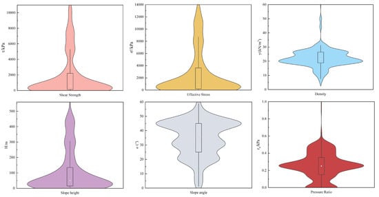
Figure 2.
Distribution of six characteristic parameters of the slope.
By calculating and visualizing the correlation coefficients of the input dataset, the Kendall correlation coefficient matrix between the six features is obtained, as shown in Figure 3. As can be seen from the figure, there is a strong correlation between variables X1, X2, and X4, that is, there is a strong positive correlation between shear strength, effective stress, and slope height, because slope height is the main linear factor affecting effective stress, and effective stress is the key to determine the shear strength. The correlation coefficients of variables X3 with X1, X2, and X4 are 0.5516, 0.5414, and 0.4459, respectively; that is, there is a moderate correlation between volume weight and shear strength, effective stress, and slope height. The correlation between X5 and X6 and other variables is weak, especially the correlation coefficient between the pore ratio and the other five variables ranges from −0.0838 to −0.1299. This is because the pore ratio is a defined slope parameter, while the other variables are inherent attributes of the slope directly or indirectly, which may lead to a weak negative correlation between the pore ratio and other parameters. In general, some parameters have a strong correlation, which means that a lot of information is shared among these features, which reduces the complexity of the model to a certain extent. On the other hand, the correlation of some parameters is weak, and the features are relatively independent, which is conducive to the model capturing more information and improving the model’s generalization ability.
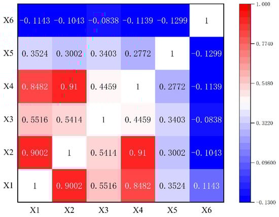
Figure 3.
Kendall correlation coefficient matrix.
4. (M-C)-BKA-MLP Prediction Model
4.1. Stability Prediction Process
- Output variable calculation
The index system based on the M-C strength criterion and the BKA-MLP model were used to predict the slope stability index–safety factor. The slope safety factor F, which was obtained by the solution of 458 groups of characteristic parameters based on the Bishop method, was taken as the output. The process of improving the MLP model using the BKA algorithm is shown in Figure 4.

Figure 4.
BKA-MLP model construction process.
- 2.
- Sample Input
A total of 458 groups of slope samples were used as datasets to train and test the prediction model. Columns one to six corresponded to a total of six input variables from X1 to X6, and the last column corresponded to the output variables of the model.
- 3.
- Sample division
Based on the size of the dataset, it is divided into the training set and the test set according to 7:3; that is, the model learns the potential law of input mapping to output on 320 datasets and makes predictions on 138 sets of previously unseen data to evaluate the model performance.
- 4.
- Cross verification
In order to make full use of data resources and fully reflect the generalization ability of the model, the model is evaluated with the fivefold cross-validation method. During each iteration, the training set is randomly divided into five parts to obtain five subsets, four of which are used for model training and the other for testing the model, and the absolute error of the BKA-MLP model on the test subset is obtained. Repeat the above process, each time selecting a different subset of the test, and finally obtain the average absolute error, which is used as the error function in the optimization process.
- 5.
- Parameter setting and optimization
The number of kites is set to 20, the maximum number of iterations of the BKA algorithm is set to 50, and the learning rate is 0.5. The number of neurons in the hidden layer and the number of iterations are optimized by the BKA algorithm. The lower bound of the optimized number of neurons is 10, the upper bound is 100, the lower bound of the iteration number is 100, and the upper bound is 1000.
- 6.
- Calculated output
Four indexes, namely the mean absolute error (MAE), mean bias error (MBE), mean square error (RMSE), and determination coefficient (R2), were used to evaluate the predictive performance of the BKA-MLP model. MAE directly reflects the absolute difference between the predicted and true values, MBE reflects systematic bias, RMSE better reflects the model’s performance in extreme cases, and R2 represents the proportion of variability explained by the model; the greater the R2, the more interpretable the model.
4.2. Model Comparison Before and After Optimization
The performance of the single MLP model was compared against that of the BKA-MLP model, with detailed results presented in Table 3. The analysis demonstrates that in comparison with the single MLP prediction model, the BKA-MLP prediction model exhibits reductions in MAE and RMSE by 0.68% and 2.3%, respectively. The relative improvements are 35.42% and 48.94%, respectively. This indicates that the optimized model has achieved substantial reductions in initial error. This indicates that the BKA-MLP model’s predictions are closer to the true values and exhibit higher accuracy. The MBE values for the two models are −0.0019 and 0.0004, respectively, indicating a negative bias of 0.19% for the MLP model and a positive bias of 0.04% for the BKA-MLP model, resulting in an absolute bias reduction of 0.15%. R2, which measures the proportion of variance explained by the model, increased by approximately 10.8% for the BKA-MLP model compared to the MLP model. This suggests that the optimized model has a superior fitting effect and can account for a larger portion of the data variability. Overall, the BKA-MLP prediction model based on the M-C strength criterion demonstrates superior performance across various metrics, showing enhanced stability and feasibility in multiple training tests.
Table 3.
MLP and BKA-MLP index results.
Figure 5 illustrates the prediction outcomes and residual analysis graphs for both the MLP model and the BKA-MLP model on the test set. From Figure 5a,c, it is evident that among approximately 140 prediction samples, the predicted safety factor values of the MLP model are notably higher than the actual values around sample numbers 10 and 30, with localized deviations observed around sample numbers 40 and 60. In contrast, the predictions from the BKA-MLP model align closely with the true values, exhibiting minimal error and superior fitting performance. Analysis of the residual plots for both models reveals that most residual errors are randomly distributed around zero, indicating no discernible trend or pattern, thus supporting the reasonableness of the linear assumption and the absence of significant heteroscedasticity. Among the 138 prediction samples, only one data point in the BKA-MLP model’s residuals exceeds ±0.1, a reduction of seven data points compared to the MLP model, resulting in a residual distribution that is more tightly clustered around zero with fewer outliers.
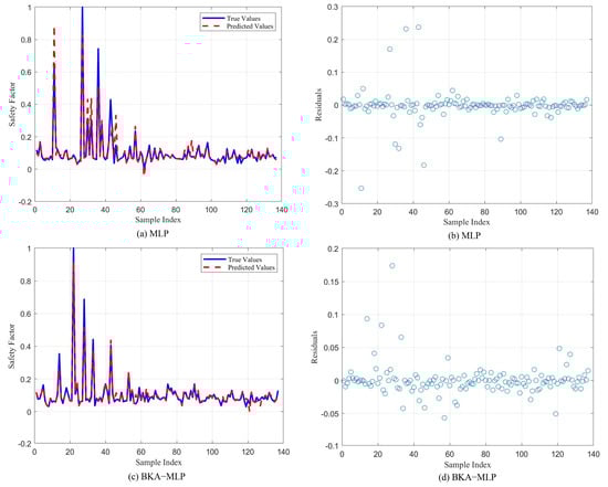
Figure 5.
Comparison of MLP and BKA-MLP results.
4.3. Comparison of the Results of Different Models
To further evaluate and benchmark the performance of the prediction models, the BKA-MLP model was compared against several established models: Random Forest Regression (RF), Support Vector Machine Regression (SVR), Long Short-Term Memory Network (LSTM), Extreme Learning Machine (ELM), and Backpropagation Neural Network (BP). The detailed performance metrics for each model are presented in Table 4. We ranked the four key performance indicators for each model and generated a radar chart to visualize the rankings of the six models, as illustrated in Figure 6. Among them, the MAE and RMSE of the BKA-MLP model are the smallest, R2 is the largest, and the MBE value is only 0.04%, although not the lowest, so the model has the best fitting effect and the highest feasibility. Second, the BP neural network prediction model, R2, and RMSE ranked second, MAE and MBE ranked third among the four indexes, and the prediction performance was slightly weaker than that of BKA-MLP. The RF prediction model and ELM prediction model have moderate ranking in the test set, average performance, and feasibility. Among all models, the LSTM and SVR prediction models have the highest MAE, MBE, and RMSE values, along with the lowest R2 values. Among these models, the error of the LSTM model is approximately one order of magnitude greater than that of the others. This discrepancy arises because the dataset primarily consists of independently distributed samples lacking pronounced time-series characteristics. Therefore, these two models have the worst performance and the lowest feasibility in predicting slope stability.
Table 4.
Results of different prediction models.
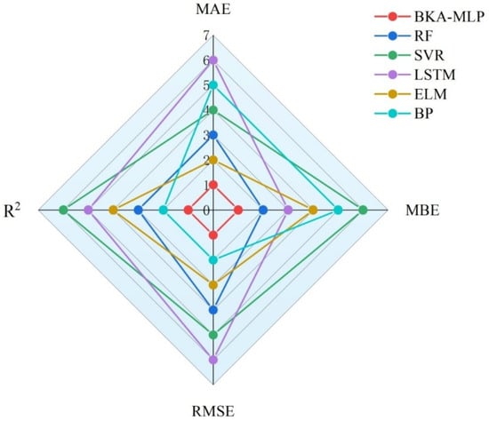
Figure 6.
Each model is ranked by four groups of indicators.
After preliminary screening, the SVR model with poor performance and the LSTM model were abandoned, and the results of the other four models with good performance on the test set were compared, as shown in Figure 7. As can be seen from the figure, the predicted value of the BKA-MLP model is the best fit with the true value, and the difference is the smallest, which indicates that the BKA-MLP prediction model has the best fitting effect and the best prediction performance. The RF model and ELM model have higher predicted values in some samples. The ELM model even has a negative safety factor when predicting data points of sample number 60, which is obviously not in line with reality. The BP neural network performed well on some samples, but the predicted value fluctuated significantly between samples 60 and 120 and was less stable than other models.
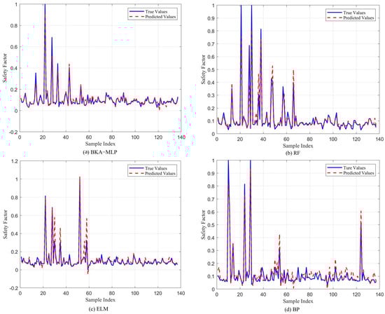
Figure 7.
Comparison of the results of the top four models.
4.4. Comparison and Verification of Different Methods
To further validate the accuracy of the BKA-MLP model’s prediction results, nine case samples were selected from the dataset. These samples encompassed three soil types—clay, sandy soil, and conglomerate—and three slope categories—gentle, moderate, and steep. The detailed classification and parameters are presented in Table 5. The limit equilibrium method and Geostudio numerical simulation were employed to calculate the safety factor for each case slope, with the results compared against those predicted by the BKA-MLP model.
Table 5.
Case classification and related parameters.
Figure 8 illustrates the comparative analysis of safety factor predictions across multiple cases using different methods. The relationship between the vertical safety factor and the horizontal case number clearly demonstrates the superiority of the BKA-MLP model. As observed from the curve trends, the correlation between the predicted and actual values of the BKA-MLP model is significantly higher than that of traditional methods, such as the limit equilibrium method and numerical simulation, particularly in high-risk cases with low safety factors (in areas where case numbers are larger). The BKA-MLP model maintains stable prediction accuracy, whereas the limit equilibrium method and conventional simulations exhibit noticeable deviations. This indicates that the BKA-MLP model can optimize MLP hyperparameters globally through the BKA algorithm, effectively addressing the limitations of traditional methods, which rely heavily on empirical parameters and lack generalization under complex conditions. Additionally, the BKA-MLP curve exhibits minimal fluctuation, suggesting robust prediction results, which are critical for engineering safety assessments. In summary, the BKA-MLP model demonstrates significant advantages in terms of prediction accuracy, stability, and adaptability to complex conditions, providing a more reliable and intelligent solution for slope geotechnical engineering stability analysis.
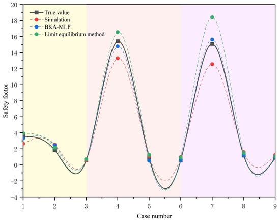
Figure 8.
Comparison of prediction results by different methods.
5. SHAP Analysis
SHAP is a method for interpreting the predictions of machine learning models [38], whose core idea is to calculate a SHAP value for each feature, representing the impact of that feature on the model’s output. Specifically, the SHAP value reflects the average change in the model’s predicted outcome when a given feature is added to the model. The calculation of SHAP values takes into account all possible feature combinations to ensure that the contribution of each feature is evaluated in all possible scenarios, thus providing a unified framework for global and local explanations.
The trained BKA-MLP prediction model computed the Shapley values based on the test set data and visualized the results, as illustrated in Figure 9 and Figure 10. From the feature importance histogram, it is evident that feature X2 has the most significant impact on the model output, with an average SHAP value of approximately 0.07. Features X1 and X5 also exhibit considerable influence, while X3 has a relatively minor impact with a SHAP value around 0.02. Contrary to the initial statement, changes in features X1 and X2 have substantial effects on the model output. Figure 10 elucidates the influence of each feature on the model’s prediction outcomes. A positive Shapley value signifies that an increase in the corresponding feature enhances the safety of the prediction, indicating a positive influence on slope stability. Conversely, negative Shapley values denote a detrimental effect. The horizontal axis illustrates the magnitude of the Shapley values; a larger Shapley value associated with a data point implies a more significant impact of that feature on slope stability. The color gradient from blue to red represents the feature values from low to high. For features X1 and X2, the distribution of sample points is relatively dispersed, and their SHAP values are notably large. When the value of X2 is low, its SHAP value is positive, indicating a positive impact on the model’s predictions. However, as the value of X2 increases, the SHAP value gradually approaches zero and transitions to a negative value, suggesting that the influence of X2 on the model initially decreases and then increases. When X2 is high, the SHAP value becomes negative, indicating a detrimental effect on the model’s prediction results. Conversely, the SHAP analysis of X1 shows a trend opposite to that of X2.
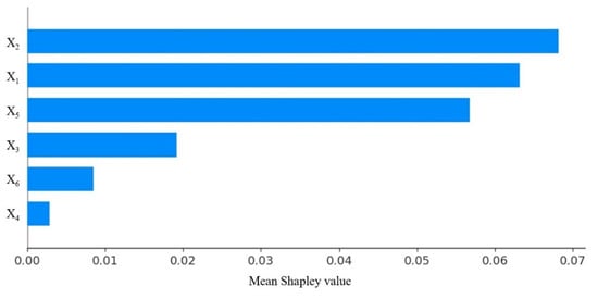
Figure 9.
Average SHAP Values for Feature Importance.
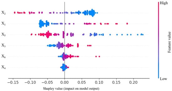
Figure 10.
Feature Importance Analysis Using SHAP Values.
From a rock mechanics perspective, an increase in shear strength enhances the deformation resistance of the slope’s rock and soil mass, thereby increasing the safety factor. This relationship is corroborated by the interaction between X1 and the predicted model in Figure 10. However, X2 exhibits both positive and negative SHAP values, implying that an increase in effective stress does not necessarily lead to an increase in the safety factor. The point distributions for the other four features are relatively concentrated, with smaller SHAP values, particularly for X4, which has the least influence on the model and predominantly negative SHAP values. In fact, an increase in slope height tends to decrease the safety factor. However, this relationship is not absolute. When the slope height is greater, the negative impact of the slope height can be mitigated by a smaller slope angle and higher effective stress, potentially resulting in an elevated safety factor. In summary, features X1 to X6 are ranked by their contribution to the model from greatest to least, and the order is X2, X1, X5, X3, X6, and X4. This indicates that the sensitivity of each feature index to the slope safety factor F follows the order σ′ (effective stress), τ (shear strength), α (slope angle), γ (unit weight), H (slope height), and ru (pore water pressure). Given the practical significance of these indices, it is clear that the effective stress and shear strength of the slope’s rock mass have the most significant influence on slope stability. Additionally, the inherent properties of the slope itself play a crucial role in determining its strength and stress characteristics. Moreover, the slope angle significantly affects slope stability. Therefore, in practical engineering applications for slope design and stability control, measures such as grouting to improve soil properties, installing drainage systems to reduce pore water pressure and increase effective stress, grading the slope to disperse loads, and setting up retaining walls can be implemented to ensure effective landslide prevention.
6. Conclusions
In this paper, a feature system integrating rock mechanics and slope stability influencing factors is constructed based on the molar Coulomb criterion. Four hundred fifty-eight datasets are calculated as input, and the slope safety factor is taken as output. A new slope stability prediction method is proposed, and the main structural parameters of the multilevel sensing neural network are optimized by the BKA algorithm. The optimal model is used for simulation tests, and the results are compared with those of other commonly used models. Finally, SHAP is used to analyze the mechanism of the influence of each feature on slope stability. The main conclusions are as follows:
- (1)
- Based on the M-C criterion, τ and σ′ are extracted as key features to construct an index system, which has more direct physical significance and interpretability.
- (2)
- The BKA-MLP model performs well in slope stability prediction, with an MAE value of 0.0124, RMSE of 0.0241, and R2 of 0.9499, all of which are better than other prediction models.
- (3)
- SHAP analysis revealed the influence mechanism of each feature on the optimal BKA-MLP prediction model from the global and local and found that the effective stress, slope inclination, and shear strength have a great influence on the occurrence of landslide; the results can provide some references for practical slope engineering applications.
- (4)
- In this study, the model primarily focuses on geotechnical mechanical properties for predicting slope stability while other nonmechanical factors are not considered. Future research could be enhanced in two main directions. Firstly, incorporating real-time variables such as rainfall intensity, seismic activity, and soil moisture content can improve the model’s adaptability to transient conditions. Secondly, exploring the feasibility of hybrid algorithms may optimize prediction accuracy, computational efficiency, and model interpretability.
Author Contributions
Methodology, Y.L.; resources, H.Z.; writing–original draft, Y.L.; data curation, Y.L.; writing—reviewing and editing, H.Z.; project administration, H.Z.; funding acquisition, H.Z. All authors have read and agreed to the published version of the manuscript.
Funding
This research was funded by the Key Science and Technology Project of the Ministry of Emergency Management of the People’s Republic of China, grant number 2024EMST080802, and by the National Key R&D Program of China, grant number 2022YFB4703701.
Institutional Review Board Statement
Not applicable.
Informed Consent Statement
Not applicable.
Data Availability Statement
The datasets generated during and/or analyzed during the current study are available from the corresponding author upon reasonable request.
Acknowledgments
The authors thank the anonymous reviewers, who provided valuable suggestions that improved the manuscript.
Conflicts of Interest
The authors declare that they have no conflicts of interest.
References
- Alcántara-Ayala, I.; Sassa, K. Landslide risk management: From hazard to disaster risk reduction. Landslides 2023, 20, 2031–2037. [Google Scholar] [CrossRef]
- Zhu, C.; Gong, Y.; Song, S.; He, M. Landslide multi-source monitoring technology and the early warning model research progress and prospect. J. Southwest Jiaotong Univ. 2024, 1–19. [Google Scholar]
- Bochao, Z.; Hui, T.; Fei, D. Research status of slope stability and intelligent monitoring technology in open-pit coal mine. China Min. Ind. 2024, 33 (Suppl. S2), 92–97. [Google Scholar]
- Asteris, P.G.; Rizal, F.I.M.; Koopialipoor, M.; Roussis, P.C.; Ferentinou, M.; Armaghani, D.J.; Gordan, B. Slope stability classification under seismic conditions using several tree-based intelligent techniques. Appl. Sci. 2022, 12, 1753. [Google Scholar] [CrossRef]
- Baghbani, A.; Choudhury, T.; Costa, S.; Reiner, J. Application of artificial intelligence in geotechnical engineering: A state-of-the-art review. Earth-Sci. Rev. 2022, 228, 103991. [Google Scholar] [CrossRef]
- Jin, A.; Zhang, J.; Sun, H.; Wang, B. Based on SSA—Slope instability of intelligent prediction and early warning model of SVM. J. Huazhong Univ. Sci. Technol. 2022, 50, 142–148. [Google Scholar] [CrossRef]
- Yan, X.; Li, X. Bayes discriminant analysis method for predicting the stability of open pit slope. In Proceedings of the 2011 International Conference on Electric Technology and Civil Engineering (ICETCE), Lushan, China, 22–24 April 2011; pp. 147–150. [Google Scholar] [CrossRef]
- Zhang, J.; Liu, Z.; Zhang, S.; Guo, T.; Yuan, C. Slope stability prediction model based on WOA-RF. Chin. J. High Press. Phys. 2019, 38, 194–205. [Google Scholar]
- Hoang, N.D.; Pham, A.D. Hybrid artificial intelligence approach based on metaheuristic and machine learning for slope stability assessment: A multinational data analysis. Expert Syst. Appl. 2016, 46, 60–68. [Google Scholar] [CrossRef]
- Sun, Y.; Yao, B.; Xu, B. Review and prospect of mine slope stability research. J. Eng. Geol. 1998, 6, 305–311. [Google Scholar]
- Sun, J.; Wu, S.; Zhang, H.; Zhang, X.; Wang, T. Based on multi-algorithm hybrid method to predict the slope safety factor--stacking ensemble learning with bayesian optimization. J. Comput. Sci. 2022, 59, 101587. [Google Scholar] [CrossRef]
- Zhang, S.; Du, H.; Fan, Y.; Sun, Q.; Pu, C. Slope stability prediction based on SSA optimization BP neural network. Transp. Sci. Technol. 2024, 6–10. [Google Scholar]
- Wang, P. Research on Stability prediction of High cut slope based on GM-RBF combination model. Build. Struct. 2021, 51, 140–145. [Google Scholar] [CrossRef]
- Zhou, X.; Wen, H.; Li, Z.; Zhang, H.; Zhang, W. An interpretable model for the susceptibility of rainfall-induced shallow landslides based on SHAP and XGBoost. Geocarto Int. 2022, 37, 13419–13450. [Google Scholar] [CrossRef]
- Zhou, C.; Yin, K.; Cao, Y.; Ahmed, B. Application of time series analysis and PSO–SVM model in predicting the Bazimen landslide in the Three Gorges Reservoir, China. Eng. Geol. 2016, 204, 108–120. [Google Scholar] [CrossRef]
- Guo, Z.; Chen, L.; Gui, L.; Du, J.; Yin, K.; Do, H.M. Landslide displacement prediction based on variational mode decomposition and WA-GWO-BP model. Landslides 2020, 17, 567–583. [Google Scholar] [CrossRef]
- Hou, K.; Bao, G.; Sun, H. SSA-MLP model in the application of the rock slope stability prediction. J. Saf. Environ. 2024, 24, 1795–1803. [Google Scholar] [CrossRef]
- Yu, Y.; Si, X.; Hu, C.; Zhang, J. A review of recurrent neural networks: LSTM cells and network architectures. Neural Comput. 2019, 31, 1235–1270. [Google Scholar] [CrossRef]
- Chauhan, V.K.; Dahiya, K.; Sharma, A. Problem formulations and solvers in linear SVM: A review. Artif. Intell. Rev. 2019, 52, 803–855. [Google Scholar] [CrossRef]
- Xie, S.; Lin, H.; Chen, Y.; Ma, T. Modified Mohr-Coulomb criterion for nonlinear strength characteristics of rocks. Fatigue Fract. Eng. Mater. Struct. 2024, 47, 2228–2242. [Google Scholar] [CrossRef]
- Shen, B.; Shi, J.; Barton, N. An approximate nonlinear modified Mohr-Coulomb shear strength criterion with critical state for intact rocks. J. Rock Mech. Geotech. Eng. 2018, 10, 645–652. [Google Scholar] [CrossRef]
- Guo, X.; Li, Y.; Cui, P.; Zhao, W.; Jiang, X.; Yan, Y. Discontinuous slope failures and pore-water pressure variation. J. Mt. Sci. 2016, 13, 116–125. [Google Scholar] [CrossRef]
- Yang, Y.; Liao, H.; Zhu, J. Stability Analysis of Three-Dimensional Tunnel Face Considering Linear and Nonlinear Strength in Unsaturated Soil. Appl. Sci. 2024, 14, 2080. [Google Scholar] [CrossRef]
- Li, C.; Zhao, X.; Xu, X.; Qu, X. Study on the differences between Hoek–Brown parameters and equivalent Mohr-Coulomb parameters in the calculation slope critical acceleration and permanent displacement. Sci. Rep. 2024, 14, 15128. [Google Scholar] [CrossRef] [PubMed]
- Wang, J.; Wang, W.; Hu, X.; Qui, L.; Zang, H. Black-winged kite algorithm: A nature-inspired meta-heuristic for solving benchmark functions and engineering problems. Artif. Intell. Rev. 2024, 57, 98. [Google Scholar] [CrossRef]
- Zhang, Z.; Wang, X.; Yue, Y. Heuristic Optimization Algorithm of Black-Winged Kite Fused with Osprey and Its Engineering Application. Biomimetics 2024, 9, 595. [Google Scholar] [CrossRef]
- Xue, R.; Zhang, X.; Xu, X.; Zhang, J.; Cheng, D.; Wang, G. Multi-strategy Integration Model Based on Black-Winged Kite Algorithm and Artificial Rabbit Optimization. In Proceedings of the International Conference on Swarm Intelligence, Singapore, 24–25 April 2024; pp. 197–207. [Google Scholar]
- Lu, P.; Rosenbaum, M.S. Artificial neural networks and grey systems for the prediction of slope stability. Nat. Hazards 2003, 30, 383–398. [Google Scholar] [CrossRef]
- Koopialipoor, M.; Asteris, P.G.; Mohammed, A.S.; Alexakis, D.E.; Mamou, A.; Armaghani, D.J. Introducing stacking machine learning approaches for the prediction of rock deformation. Transp. Geotech. 2022, 34, 100756. [Google Scholar] [CrossRef]
- Lin, R.; Zhou, Z.; You, S.; Rao, R.; Kuo, C.-C.J. Geometrical interpretation and design of multilayer perceptrons. IEEE Trans. Neural Netw. Learn. Syst. 2022, 35, 2545–2559. [Google Scholar] [CrossRef]
- Huang, F.; Cao, Z.; Jiang, S.H.; Zhou, C.; Huang, J.; Guo, Z. Landslide susceptibility prediction based on a semi-supervised multiple-layer perceptron model. Landslides 2020, 17, 2919–2930. [Google Scholar] [CrossRef]
- Moayedi, H.; Canatalay, P.J.; Ahmadi Dehrashid, A.; Cifci, M.A.; Salari, M.; Le, B.N. Multilayer perceptron and their comparison with two nature-inspired hybrid techniques of biogeography-based optimization (BBO) and backtracking search algorithm (BSA) for assessment of landslide susceptibility. Land 2023, 12, 242. [Google Scholar] [CrossRef]
- Zhao, H.; Du, H.; Su, H.; Li, M. Open-pit mine compound soft rock slope of coal seam bottom friction experimental study. J. Coal 2018, 2724–2731. [Google Scholar] [CrossRef]
- Shi, X.; Zhou, J.; Zheng, W.; Hu, H.; Wang, H. Bayes discriminant analysis method for prediction of slope stability and its application. J. Sichuan Univ. 2010, 42, 63–68. [Google Scholar] [CrossRef]
- Su, G.; Song, Y.; Yan, L. Gaussian process machine learning application in slope stability evaluation. Rock Soil Mech. 2009, 30, 675–679+687. [Google Scholar]
- Zhang, Y. Slope stability based on GS—The SVM prediction model. J. Water Resour. Hydropower Technol. 2020, 51, 205–209. [Google Scholar]
- Wang, J.; Xu, Y.; Li, J. Slope stability coefficient prediction based on grid search support vector Machine. Railw. Constr. 2019, 59, 94–97. [Google Scholar]
- Van den Broeck, G.; Lykov, A.; Schleich, M.; Suciu, D. On the tractability of SHAP explanations. J. Artif. Intell. Res. 2022, 74, 851–886. [Google Scholar] [CrossRef]
Disclaimer/Publisher’s Note: The statements, opinions and data contained in all publications are solely those of the individual author(s) and contributor(s) and not of MDPI and/or the editor(s). MDPI and/or the editor(s) disclaim responsibility for any injury to people or property resulting from any ideas, methods, instructions or products referred to in the content. |
© 2025 by the authors. Licensee MDPI, Basel, Switzerland. This article is an open access article distributed under the terms and conditions of the Creative Commons Attribution (CC BY) license (https://creativecommons.org/licenses/by/4.0/).