
Analyzing LLAMA3 Performance on Classification Task Using LoRA and QLoRA Techniques


Abstract
1. Introduction
1.1. Motivation
1.2. Background
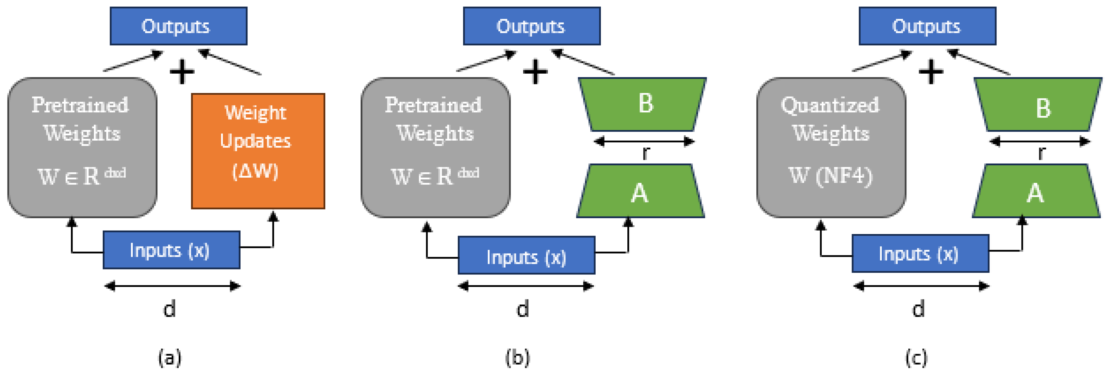
1.2.1. LoRA
1.2.2. QLoRA
1.3. Contributions
- 1.
- The article analyzes the improvement obtained over the base LLaMA3-8B model using two PEFT techniques—LoRA and QLoRA;
- 2.
- It also explores the effects of hyperparameter adjustments (r and ) on the model’s performance to find the optimal values of r and for the classification task;
- 3.
- The paper examines the tradeoff between efficiency and memory savings obtained using the quantized technique over LoRA;
- 4.
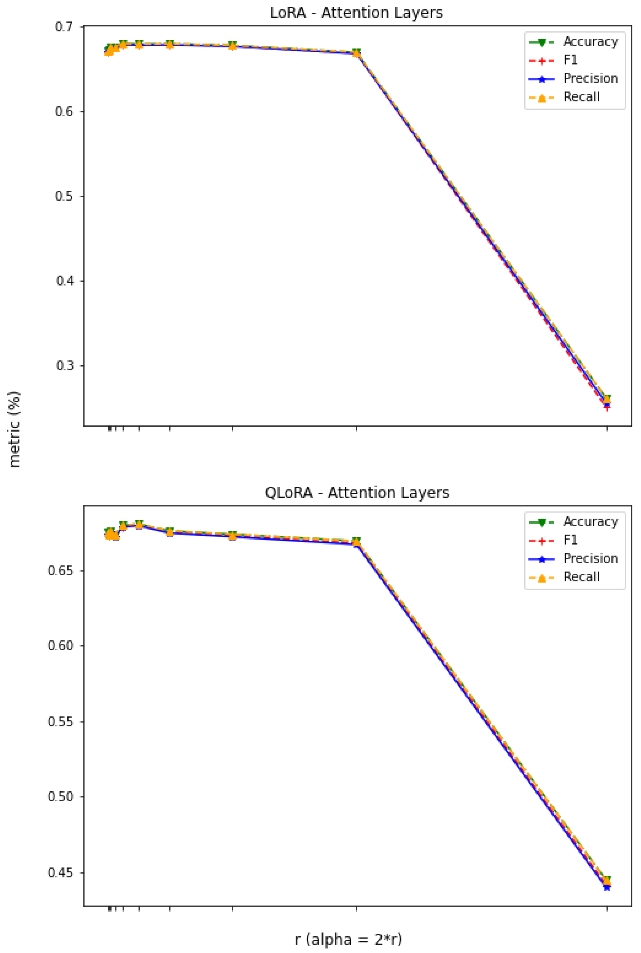
- It also investigates and compares the change in the performance obtained after the adaptation of the attention layers (query, key, value, and project) versus all the linear layers during fine tuning at LoRA and QLoRA settings;
- 5.
- Finally, the article experiments with the usage of the decoder-based Llama-3-8B model for classification tasks, such as sentiment analysis.
2. Methodology
2.1. Model and Task
2.2. Dataset and Setup
2.3. Hardware, Time, and Memory
2.4. Selection of Hyperparameters
2.5. Computational Efficiency During Inference and Training
2.5.1. Memory Estimation for Inferences
2.5.2. Memory Estimation for Training
2.6. Comparative Analysis of LoRA and QLoRA Techniques
2.6.1. LoRA
2.6.2. QLoRA
2.7. Strategy
3. Experiments and Results
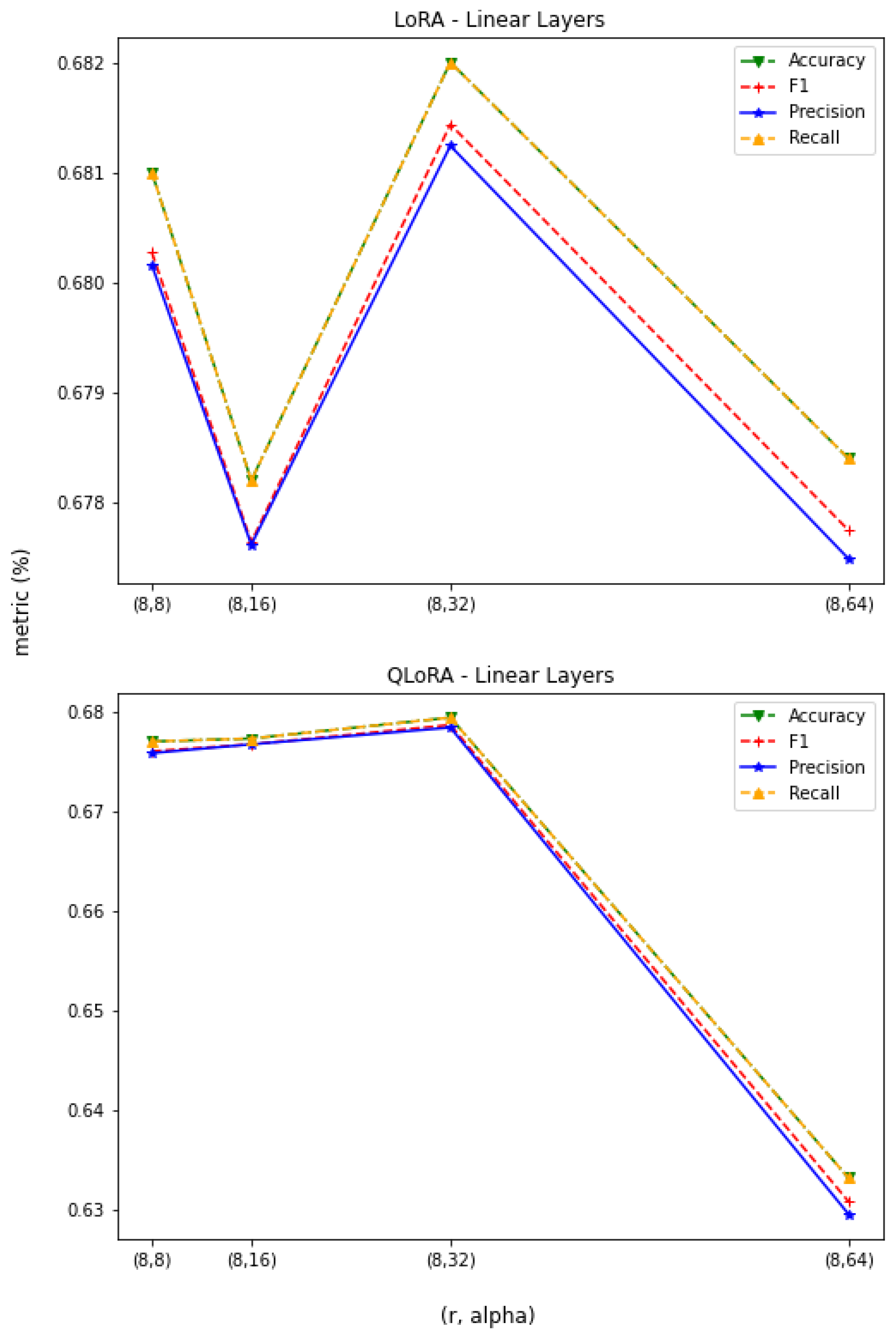
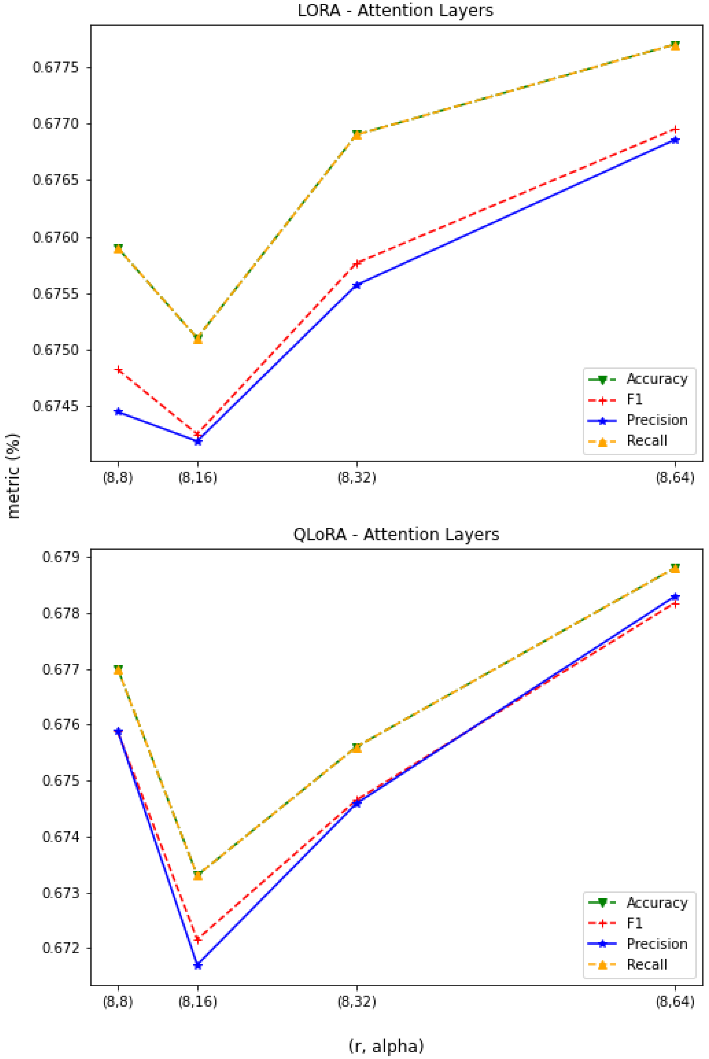
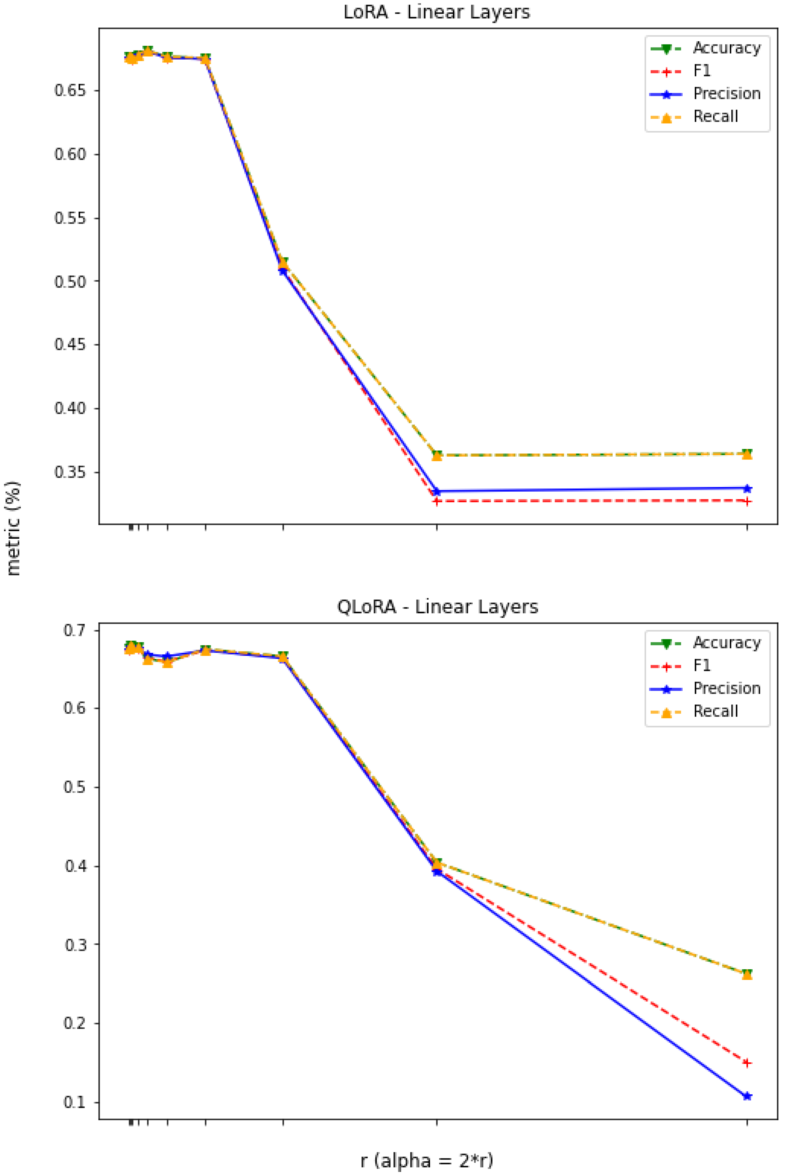
3.1. Constant r
3.2. Constant
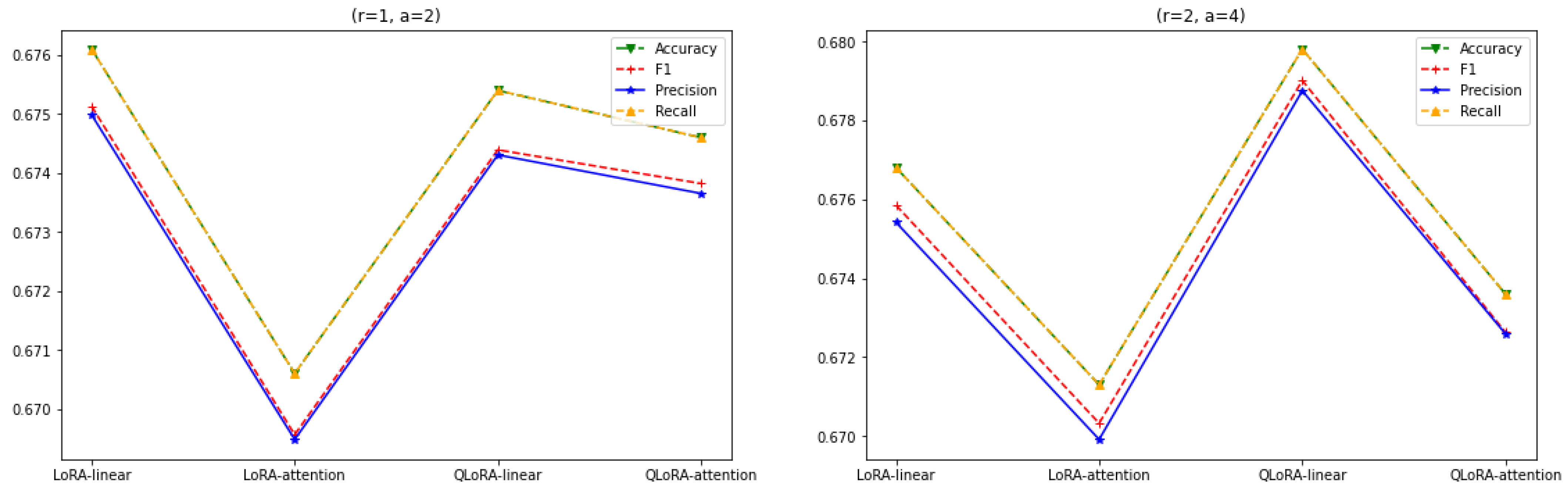
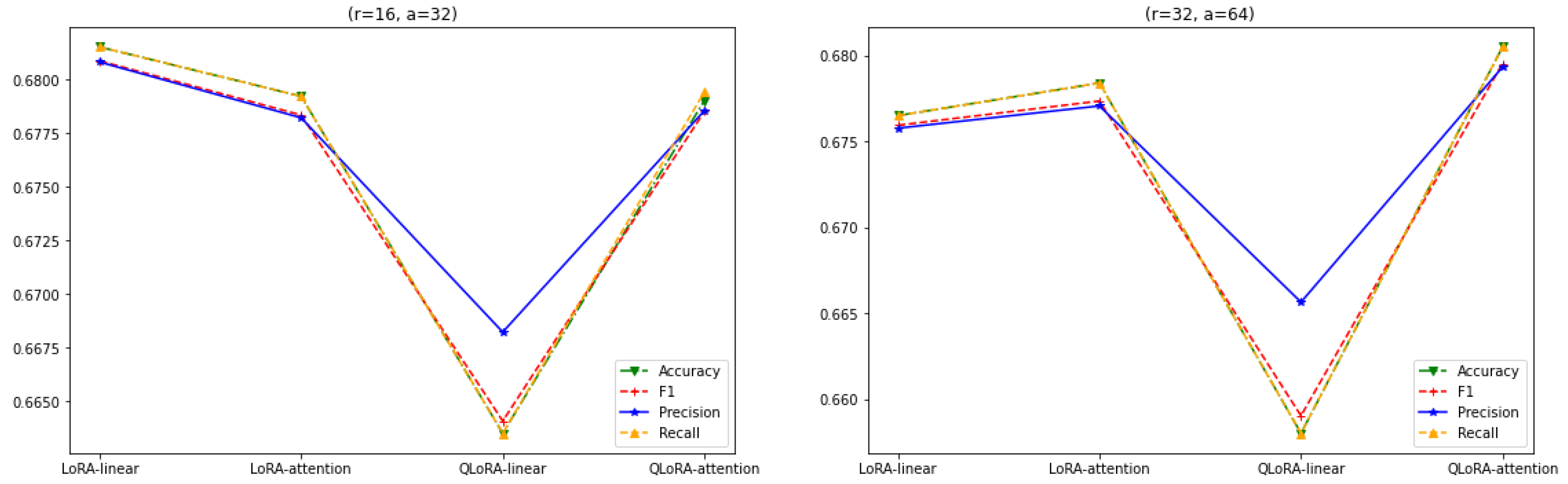
3.3. LoRA vs. QLoRA Performance
3.4. Scope
4. Related Work
4.1. PEFTs
4.2. Reparameterization Methods
4.3. Adapter Tuning
4.4. Prompt-Based Methods
4.4.1. Prompt Tuning
4.4.2. Prefix Tuning
4.4.3. P-Tuning
5. Conclusions
Author Contributions
Funding
Institutional Review Board Statement
Informed Consent Statement
Data Availability Statement
Conflicts of Interest
References
- Vaswani, A.; Shazeer, N.; Parmar, N.; Uszkoreit, J.; Jones, L.; Gomez, A.N.; Kaiser, Ł.; Polosukhin, I. Attention Is All You Need. Advances in Neural Information Processing Systems. 2017. Available online: https://proceedings.neurips.cc/paper/2017/hash/3f5ee243547dee91fbd053c1c4a845aa-Abstract.html (accessed on 15 February 2025).
- Raffel, C.; Shazeer, N.; Roberts, A.; Lee, K.; Narang, S.; Matena, M.; Zhou, Y.; Li, W.; Liu, P.J. Exploring the limits of transfer learning with a unified text-to-text transformer. J. Mach. Learn. Res. 2020, 21, 5485–5551. [Google Scholar]
- Devlin, J.; Chang, M.W.; Lee, K.; Toutanova, K. Bert: Pre-training of deep bidirectional transformers for language understanding. arXiv 2018, arXiv:1810.04805. [Google Scholar]
- Brown, T.; Mann, B.; Ryder, N.; Subbiah, M.; Kaplan, J.D.; Dhariwal, P.; Neelakantan, A.; Shyam, P.; Sastry, G.; Askell, A.; et al. Language models are few-shot learners. Adv. Neural Inf. Process. Syst. 2020, 33, 1877–1901. [Google Scholar]
- Achiam, J.; Adler, S.; Agarwal, S.; Ahmad, L.; Akkaya, I.; Aleman, F.L.; Almeida, D.; Altenschmidt, J.; Altman, S.; Anadkat, S.; et al. Gpt-4 technical report. arXiv 2023, arXiv:2303.08774. [Google Scholar]
- Touvron, H.; Lavril, T.; Izacard, G.; Martinet, X.; Lachaux, M.A.; Lacroix, T.; Rozière, B.; Goyal, N.; Hambro, E.; Azhar, F.; et al. Llama: Open and efficient foundation language models. arXiv 2023, arXiv:2302.13971. [Google Scholar]
- Zhang, S.; Roller, S.; Goyal, N.; Artetxe, M.; Chen, M.; Chen, S.; Dewan, C.; Diab, M.; Li, X.; Lin, X.V.; et al. Opt: Open pre-trained transformer language models. arXiv 2022, arXiv:2205.01068. [Google Scholar]
- Wei, J.; Wang, X.; Schuurmans, D.; Bosma, M.; Xia, F.; Chi, E.; Le, Q.V.; Zhou, D. Chain-of-thought prompting elicits reasoning in large language models. Adv. Neural Inf. Process. Syst. 2022, 35, 24824–24837. [Google Scholar]
- Dong, Q.; Li, L.; Dai, D.; Zheng, C.; Wu, Z.; Chang, B.; Sun, X.; Xu, J.; Sui, Z. A survey on in-context learning. arXiv 2022, arXiv:2301.00234. [Google Scholar]
- Wang, T.; Roberts, A.; Hesslow, D.; Le Scao, T.; Chung, H.W.; Beltagy, I.; Launay, J.; Raffel, C. What language model architecture and pretraining objective works best for zero-shot generalization? In Proceedings of the International Conference on Machine Learning, PMLR, Online, 28–30 March 2022; pp. 22964–22984. [Google Scholar]
- Introducing Meta Llama 3: The Most Capable Openly Available LLM to Date. Available online: https://huggingface.co/meta-llama/Meta-Llama-3-8B (accessed on 15 November 2024).
- Houlsby, N.; Giurgiu, A.; Jastrzebski, S.; Morrone, B.; De Laroussilhe, Q.; Gesmundo, A.; Attariyan, M.; Gelly, S. Parameter-efficient transfer learning for NLP. In Proceedings of the International Conference on Machine Learning, PMLR, Long Beach, CA, USA, 10–15 June 2019; pp. 2790–2799. [Google Scholar]
- Patterson, D.; Gonzalez, J.; Le, Q.; Liang, C.; Munguia, L.M.; Rothchild, D.; So, D.; Texier, M.; Dean, J. Carbon emissions and large neural network training. arXiv 2021, arXiv:2104.10350. [Google Scholar]
- Hu, E.J.; Shen, Y.; Wallis, P.; Allen-Zhu, Z.; Li, Y.; Wang, S.; Wang, L.; Chen, W. Lora: Low-rank adaptation of large language models. arXiv 2021, arXiv:2106.09685. [Google Scholar]
- Dettmers, T.; Pagnoni, A.; Holtzman, A.; Zettlemoyer, L. Qlora: Efficient finetuning of quantized llms. Adv. Neural Inf. Process. Syst. 2023, 36, 10088–10115. [Google Scholar]
- Li, C.; Farkhoor, H.; Liu, R.; Yosinski, J. Measuring the intrinsic dimension of objective landscapes. arXiv 2018, arXiv:1804.08838. [Google Scholar]
- Aghajanyan, A.; Zettlemoyer, L.; Gupta, S. Intrinsic dimensionality explains the effectiveness of language model fine-tuning. arXiv 2020, arXiv:2012.13255. [Google Scholar]
- Zhang, X.; Zhao, J.; LeCun, Y. Character-level Convolutional Networks for Text Classification, Advances in Neural Information Processing Systems, 28, NIPS 2015. Available online: https://proceedings.neurips.cc/paper/2015/hash/250cf8b51c773f3f8dc8b4be867a9a02-Abstract.html (accessed on 15 February 2025).
- Yu, Z.; Ananiadou, S. Neuron-level knowledge attribution in large language models. In Proceedings of the 2024 Conference on Empirical Methods in Natural Language Processing, Miami, FL, USA, 12–16 November 2024; pp. 3267–3280. [Google Scholar]
- Zheng, Z.; Wang, Y.; Huang, Y.; Song, S.; Yang, M.; Tang, B.; Xiong, F.; Li, Z. Attention heads of large language models: A survey. arXiv 2024, arXiv:2409.03752. [Google Scholar] [CrossRef]
- Zhang, Q.; Chen, M.; Bukharin, A.; He, P.; Cheng, Y.; Chen, W.; Zhao, T. AdaLoRA: Adaptive budget allocation for parameter-efficient fine-tuning. arXiv 2023, arXiv:2303.10512. [Google Scholar]
- Liu, H.; Tam, D.; Muqeeth, M.; Mohta, J.; Huang, T.; Bansal, M.; Raffel, C.A. Few-shot parameter-efficient fine-tuning is better and cheaper than in-context learning. Adv. Neural Inf. Process. Syst. 2022, 35, 1950–1965. [Google Scholar]
- Hyeon-Woo, N.; Ye-Bin, M.; Oh, T.H. Fedpara: Low-rank hadamard product for communication-efficient federated learning. arXiv 2021, arXiv:2108.06098. [Google Scholar]
- Valipour, M.; Rezagholizadeh, M.; Kobyzev, I.; Ghodsi, A. Dylora: Parameter efficient tuning of pre-trained models using dynamic search-free low-rank adaptation. arXiv 2022, arXiv:2210.07558. [Google Scholar]
- Liu, S.Y.; Wang, C.Y.; Yin, H.; Molchanov, P.; Wang, Y.C.F.; Cheng, K.T.; Chen, M.H. Dora: Weight-decomposed low-rank adaptation. arXiv 2024, arXiv:2402.09353. [Google Scholar]
- Chavan, A.; Liu, Z.; Gupta, D.; Xing, E.; Shen, Z. One-for-all: Generalized lora for parameter-efficient fine-tuning. arXiv 2023, arXiv:2306.07967. [Google Scholar]
- Edalati, A.; Tahaei, M.; Kobyzev, I.; Nia, V.P.; Clark, J.J.; Rezagholizadeh, M. Krona: Parameter efficient tuning with kronecker adapter. arXiv 2022, arXiv:2212.10650. [Google Scholar]
- Mahabadi, R.K.; Henderson, J.; Ruder, S. Compacter: Efficient low-rank hypercomplex adapter layers. Adv. Neural Inf. Process. Syst. 2021, 34, 1022–1035. [Google Scholar]
- Newman, B.; Choubey, P.K.; Rajani, N. P-adapters: Robustly extracting factual information from language models with diverse prompts. arXiv 2021, arXiv:2110.07280. [Google Scholar]
- Lester, B.; Al-Rfou, R.; Constant, N. The power of scale for parameter-efficient prompt tuning. arXiv 2021, arXiv:2104.08691. [Google Scholar]
- Li, X.L.; Liang, P. Prefix-tuning: Optimizing continuous prompts for generation. arXiv 2021, arXiv:2101.00190. [Google Scholar]
- Zhang, R.; Han, J.; Liu, C.; Gao, P.; Zhou, A.; Hu, X.; Yan, S.; Lu, P.; Li, H.; Qiao, Y. Llama-adapter: Efficient fine-tuning of language models with zero-init attention. arXiv 2023, arXiv:2303.16199. [Google Scholar]
- Liu, X.; Zheng, Y.; Du, Z.; Ding, M.; Qian, Y.; Yang, Z.; Tang, J. GPT Understands, Too. AI Open 2024, 5, 208–215. [Google Scholar] [CrossRef]


| Method | Hardware | Time Taken for Fine Tuning | Memory Consumed |
|---|---|---|---|
| LoRA (All-Linear and Attention Layers) | 1 × A100 40 GB | 30 min | 16 GB |
| QLoRA (All-Linear and Attention Layers) | 1 × A100 40 GB | 5 h | 6 GB |
| Memory | FP32 | FP16 | int8 | int4 |
|---|---|---|---|---|
| Fine Tuning | 119.2 GB | 59.6 GB | 29.8 GB | 14.9 GB |
| Inferences | 29.80 GB | 14.90 GB | 7.45 GB | 3.73 GB |
| Type | Model Weight (Inferences) | Trainable Parameters | Gradients | AdamW | Memory for Fine Tuning |
|---|---|---|---|---|---|
| LoRA (FP32) | 29.80 GB (8 Billion × 4) | 21,024,808 × 4 bytes (0.078 GB) | 21,024,808 × 4 bytes (0.078 GB) | 21,024,808 × 8 bytes (0.157 GB) | 30.113 GB |
| LoRA (FP16) | 14.9 GB (8 Billion × 2) | 21,024,808 × 2 bytes (0.039 GB) | 21,024,808 × 4 bytes (0.078 GB) | 21,024,808 × 4 bytes (0.078 GB) | 15.095 GB |
| QLoRA (NF4) | 3.73 GB (8 Billion × 0.5) | 21,024,808 × 0.5 bytes (0.0097 GB) | 21,024,808 × 4 bytes (0.078 GB) | 21,024,808 × 2 bytes (0.039 GB) | 3.857 GB |
| r | Linear-Layer Parameters | Attention-Layer Parameters |
|---|---|---|
| 8 | 21,024,808 (0.2794%) | 6,836,224 (0.0910%) |
| 16 | 42,029,136 (0.5569%) | 13,651,968 (0.1816%) |
| 32 | 84,037,792 (1.1073%) | 27,283,456 (0.3622%) |
| 64 | 168,055,104 (2.1901%) | 54,546,432 (0.7216%) |
| 128 | 336,089,728 (4.2860%) | 109,072,384 (1.4325%) |
| 256 | 672,158,976 (8.2190%) | 218,124,288 (2.8243%) |
| 512 | 1,344,297,472 (15.1875%) | 436,228,096 (5.4932%) |
| Precision | Recall | F1-Score | Accuracy |
|---|---|---|---|
| 0.203 | 0.2191 | 0.181 | 0.2191 |
Disclaimer/Publisher’s Note: The statements, opinions and data contained in all publications are solely those of the individual author(s) and contributor(s) and not of MDPI and/or the editor(s). MDPI and/or the editor(s) disclaim responsibility for any injury to people or property resulting from any ideas, methods, instructions or products referred to in the content. |
© 2025 by the authors. Licensee MDPI, Basel, Switzerland. This article is an open access article distributed under the terms and conditions of the Creative Commons Attribution (CC BY) license (https://creativecommons.org/licenses/by/4.0/).
Share and Cite
Patil, R.; Khot, P.; Gudivada, V. Analyzing LLAMA3 Performance on Classification Task Using LoRA and QLoRA Techniques. Appl. Sci. 2025, 15, 3087. https://doi.org/10.3390/app15063087
Patil R, Khot P, Gudivada V. Analyzing LLAMA3 Performance on Classification Task Using LoRA and QLoRA Techniques. Applied Sciences. 2025; 15(6):3087. https://doi.org/10.3390/app15063087
Chicago/Turabian StylePatil, Rajvardhan, Priyanka Khot, and Venkat Gudivada. 2025. "Analyzing LLAMA3 Performance on Classification Task Using LoRA and QLoRA Techniques" Applied Sciences 15, no. 6: 3087. https://doi.org/10.3390/app15063087
APA StylePatil, R., Khot, P., & Gudivada, V. (2025). Analyzing LLAMA3 Performance on Classification Task Using LoRA and QLoRA Techniques. Applied Sciences, 15(6), 3087. https://doi.org/10.3390/app15063087