
Bi-Objective Optimization for Joint Time-Invariant Allocation of Berths and Quay Cranes


Abstract
1. Introduction
2. Literature Review
2.1. Berth Allocation Problem
2.2. Quay Crane Assignment Problem
2.3. Joint Allocation of Berths and Quay Cranes
3. Description and Formulation of BACASP
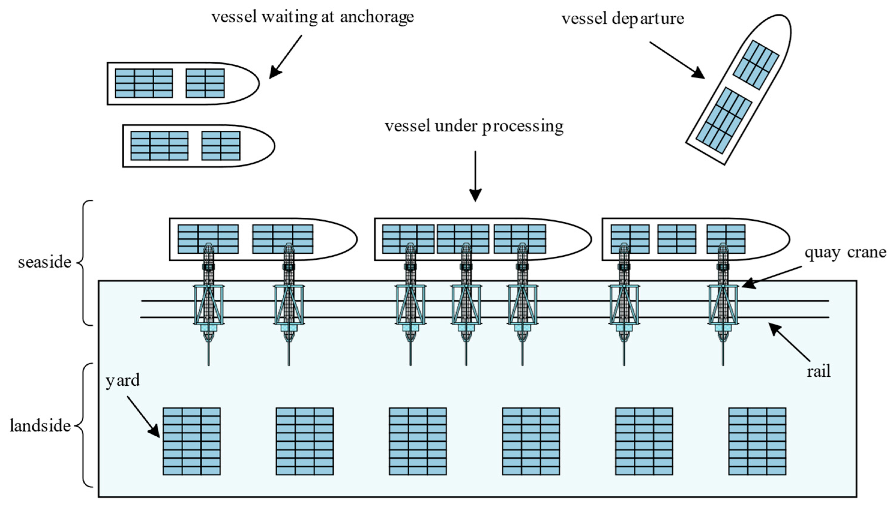
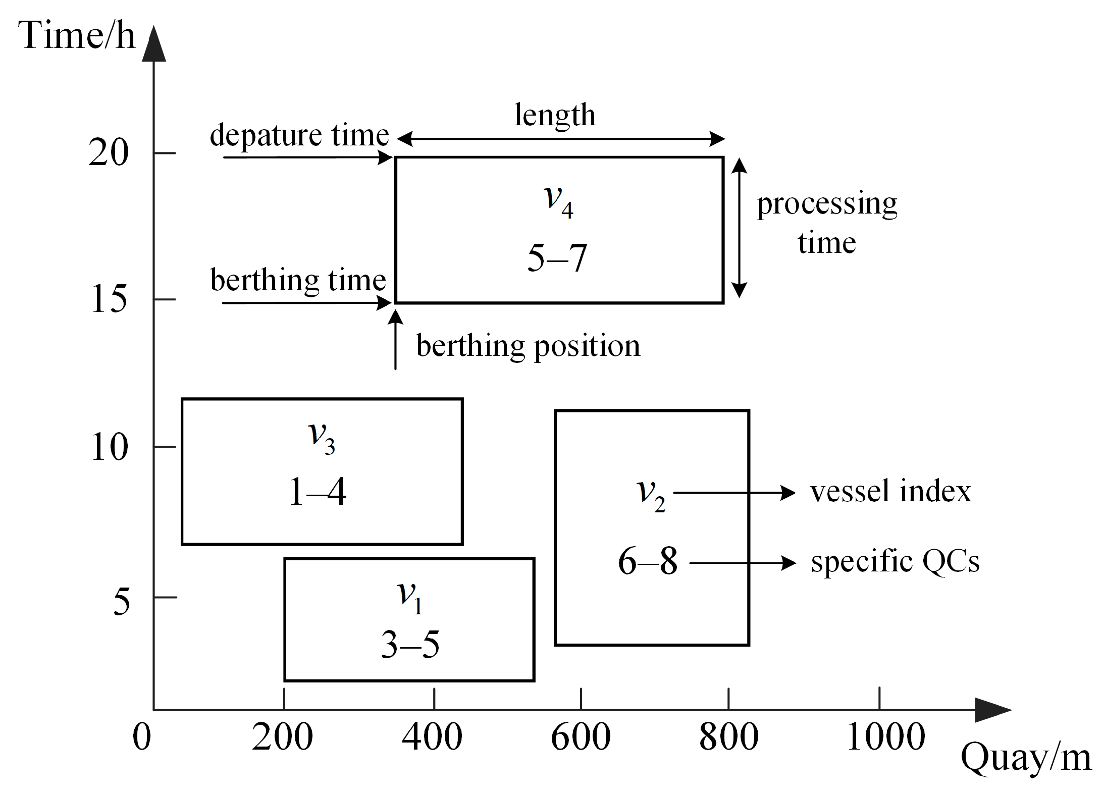
3.1. Problem Description
3.2. Assumptions and Constraints
- Each vessel cannot berth prior to arrival time and cannot berth outside the quay;
- Once berthed, a vessel cannot interrupt its processing and change its position;
- The safety distance is included in the length of each vessel;
- The processing time of each vessel is related to the berthing position and the number of assigned QCs;
- The number of QCs assigned to each vessel remains constant during its processing, which is referred to as a time-invariant assignment;
- Each vessel has a minimal and maximal number of QCs that can be assigned;
- Each position at the terminal is occupied by one vessel, at most, at any moment;
- The QCs can move along the rail but cannot cross each other.
3.3. Mathematical Formulation
4. An IMOCS Algorithm for the BACASP
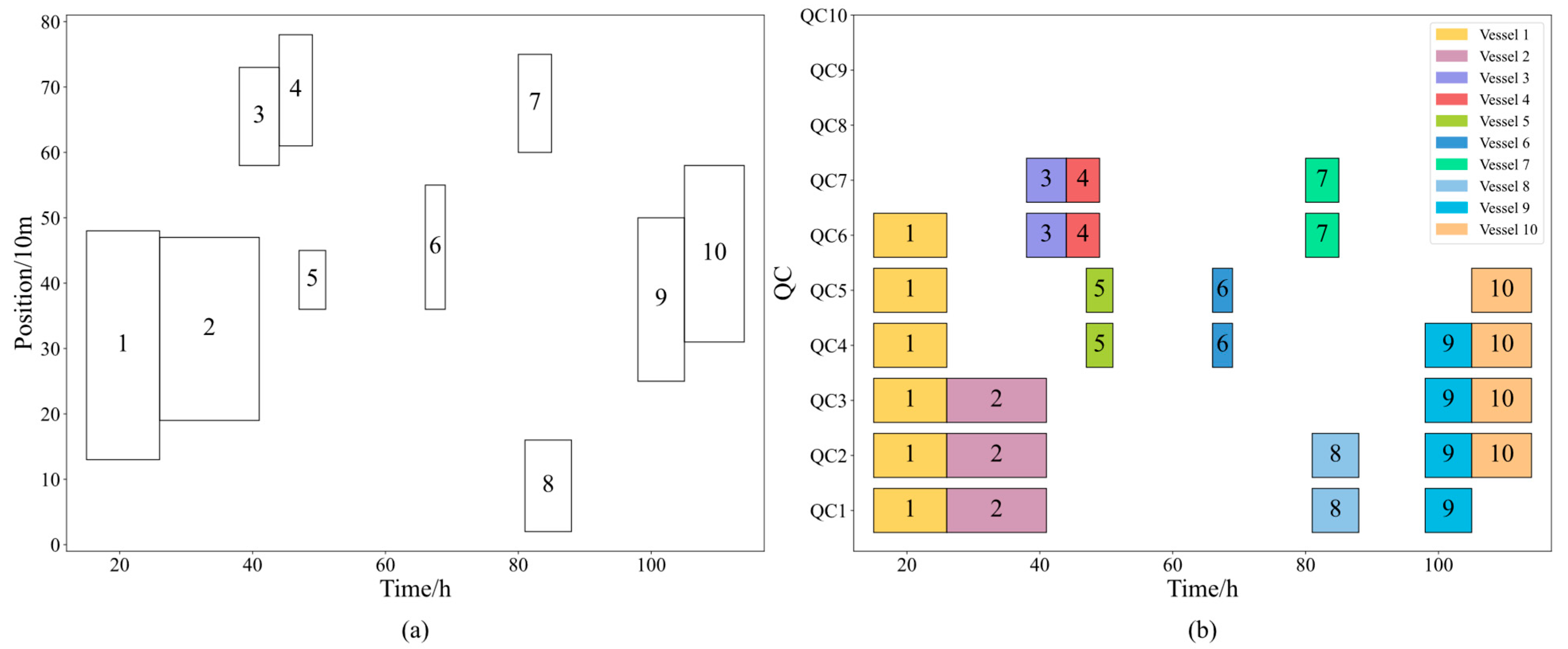
4.1. Solution Representation
| Algorithm 1. A constructive algorithm for BACASP |
 |
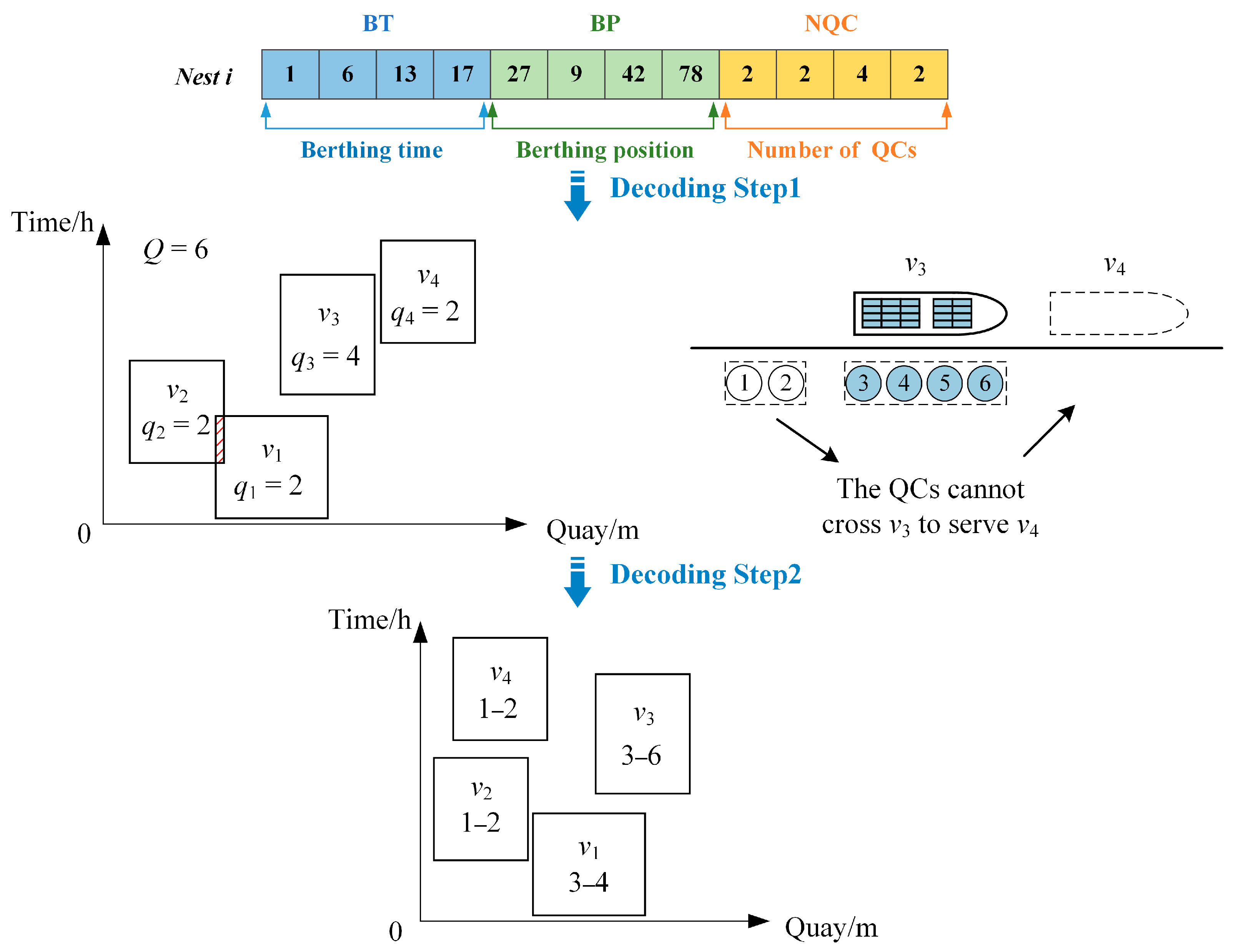
- , . is the vessel with the earliest berthing time in , so the closest available QCs, 3–4, are assigned to ;
- , . is the vessel with the earliest berthing time in and overlaps with , so adjust the berthing position and allocate continuous available berth segments to , then the closest available QCs, 1–2, are assigned to ;
- , . is the vessel with the earliest berthing time in , so the closest available QCs, 3–6, are assigned to ;
- , . is the vessel with the earliest berthing time in and the QCs cannot cross to serve , so adjust the berthing position and allocate the continuous available berth segments to , then the closest available QCs, 1–2, are assigned to .
4.2. The Initial Feasible Solution
4.3. The Dynamic Adaptive Mechanism
4.3.1. Elite Guided Adaptive Tangent Flight
4.3.2. Information-Enhanced Adaptive Abandonment Process
5. Numerical Experiments
5.1. Experiment Settings
5.1.1. Instances Generation and Parameter Setting
5.1.2. Performance Metrics
5.2. Results and Analysis
5.2.1. Performance Comparison Between IMOCS and GUROBI
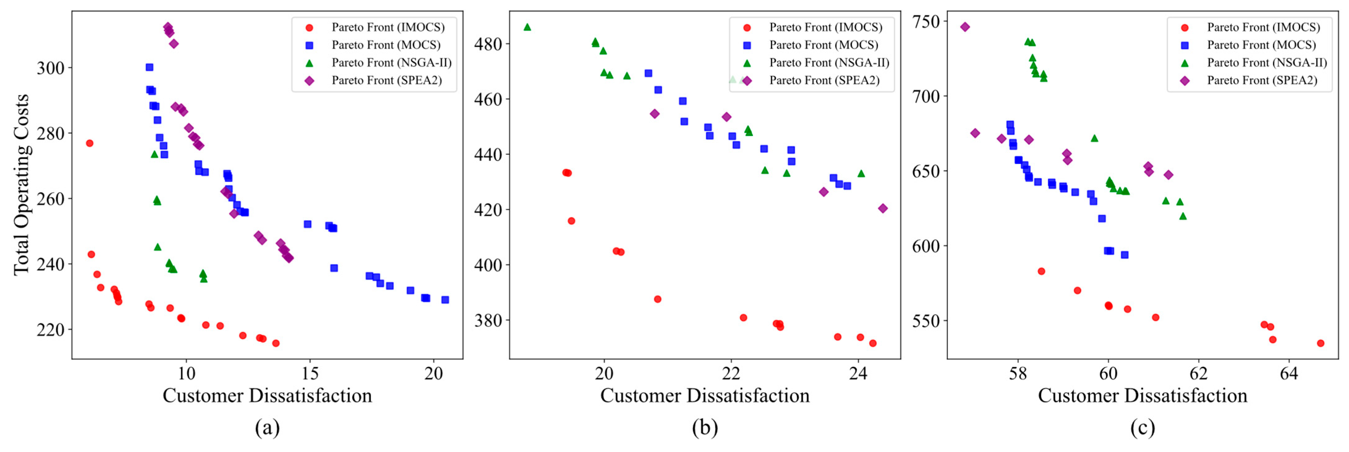
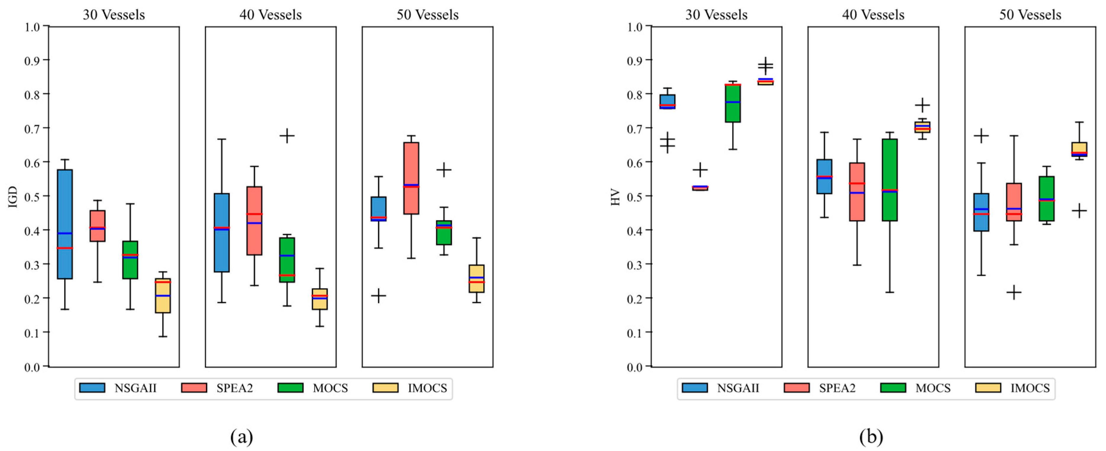
5.2.2. Performance Comparison Between IMOCS and Other Algorithms
5.2.3. Managerial Insight
6. Conclusions
Author Contributions
Funding
Institutional Review Board Statement
Informed Consent Statement
Data Availability Statement
Acknowledgments
Conflicts of Interest
References
- United Nations Conference on Trade and Development. Review of Maritime Transport 2022. 2022. Available online: https://unctad.org/system/files/official-document/rmt2022_en.pdf (accessed on 8 March 2025).
- Khadka, K.; Maharjan, S. Customer Satisfaction and Customer Loyalty. Centria Univ. Appl. Sci. Pietarsaari 2017, 1, 58–64. [Google Scholar]
- Rodrigues, F.; Agra, A. Berth Allocation and Quay Crane Assignment/Scheduling Problem under Uncertainty: A Survey. Eur. J. Oper. Res. 2022, 303, 501–524. [Google Scholar] [CrossRef]
- Cheimanoff, N.; Fontane, F.; Kitri, M.N.; Tchernev, N. Exact and Heuristic Methods for the Integrated Berth Allocation and Specific Time-Invariant Quay Crane Assignment Problems. Comput. Oper. Res. 2022, 141, 105695. [Google Scholar] [CrossRef]
- Iris, Ç.; Pacino, D.; Ropke, S.; Larsen, A. Integrated Berth Allocation and Quay Crane Assignment Problem: Set Partitioning Models and Computational Results. Transp. Res. Part E Logist. Transp. Rev. 2015, 81, 75–97. [Google Scholar] [CrossRef]
- Aslam, S.; Michaelides, M.P.; Herodotou, H. Berth Allocation Considering Multiple Quays: A Practical Approach Using Cuckoo Search Optimization. J. Mar. Sci. Eng. 2023, 11, 1280. [Google Scholar] [CrossRef]
- Ou, X.; Wu, M.; Tu, B.; Zhang, G.; Li, W. Multi-Objective Unsupervised Band Selection Method for Hyperspectral Images Classification. IEEE Trans. Image Process. 2023, 32, 1952–1965. [Google Scholar] [CrossRef]
- Song, P.-C.; Pan, J.-S.; Chu, S.-C. A Parallel Compact Cuckoo Search Algorithm for Three-Dimensional Path Planning. Appl. Soft Comput. 2020, 94, 106443. [Google Scholar] [CrossRef]
- Golias, M.M.; Boile, M.; Theofanis, S. Berth Scheduling by Customer Service Differentiation: A Multi-Objective Approach. Transp. Res. Part E Logist. Transp. Rev. 2009, 45, 878–892. [Google Scholar] [CrossRef]
- Umang, N.; Bierlaire, M.; Vacca, I. Exact and Heuristic Methods to Solve the Berth Allocation Problem in Bulk Ports. Transp. Res. Part E Logist. Transp. Rev. 2013, 54, 14–31. [Google Scholar] [CrossRef]
- Venturini, G.; Iris, Ç.; Kontovas, C.A.; Larsen, A. The Multi-Port Berth Allocation Problem with Speed Optimization and Emission Considerations. Transp. Res. Part D Transp. Environ. 2017, 54, 142–159. [Google Scholar] [CrossRef]
- Iris, Ç.; Lalla-Ruiz, E.; Lam, J.S.L.; Voß, S. Mathematical Programming Formulations for the Strategic Berth Template Problem. Comput. Ind. Eng. 2018, 124, 167–179. [Google Scholar] [CrossRef]
- Rodrigues, F. Improved Sequential Insertion Heuristics for Berth Allocation Problems. Int. Trans. Oper. Res. 2024, 31, 1585–1608. [Google Scholar] [CrossRef]
- Meisel, F. The Quay Crane Scheduling Problem with Time Windows. Nav. Res. Logist. (NRL) 2011, 58, 619–636. [Google Scholar] [CrossRef]
- Liang, C.; Huang, Y.; Yang, Y. A Quay Crane Dynamic Scheduling Problem by Hybrid Evolutionary Algorithm for Berth Allocation Planning. Comput. Ind. Eng. 2009, 56, 1021–1028. [Google Scholar] [CrossRef]
- Chargui, K.; Zouadi, T.; El Fallahi, A.; Reghioui, M.; Aouam, T. Berth and Quay Crane Allocation and Scheduling with Worker Performance Variability and Yard Truck Deployment in Container Terminals. Transp. Res. Part E Logist. Transp. Rev. 2021, 154, 102449. [Google Scholar] [CrossRef]
- Rodrigues, F.; Agra, A. Handling Uncertainty in the Quay Crane Scheduling Problem: A Unified Distributionally Robust Decision Model. Int. Trans. Oper. Res. 2024, 31, 721–748. [Google Scholar] [CrossRef]
- Meisel, F.; Bierwirth, C. Heuristics for the Integration of Crane Productivity in the Berth Allocation Problem. Transp. Res. Part E Logist. Transp. Rev. 2009, 45, 196–209. [Google Scholar] [CrossRef]
- Türkoğulları, Y.B.; Taşkın, Z.C.; Aras, N.; Altınel, İ.K. Optimal Berth Allocation, Time-Variant Quay Crane Assignment and Scheduling with Crane Setups in Container Terminals. Eur. J. Oper. Res. 2016, 254, 985–1001. [Google Scholar] [CrossRef]
- Iris, Ç.; Pacino, D.; Ropke, S. Improved Formulations and an Adaptive Large Neighborhood Search Heuristic for the Integrated Berth Allocation and Quay Crane Assignment Problem. Transp. Res. Part E Logist. Transp. Rev. 2017, 105, 123–147. [Google Scholar] [CrossRef]
- Jiao, X.; Zheng, F.; Liu, M.; Xu, Y. Integrated Berth Allocation and Time-Variant Quay Crane Scheduling with Tidal Impact in Approach Channel. Discret. Dyn. Nat. Soc. 2018, 2018, 9097047. [Google Scholar] [CrossRef]
- Iris, Ç.; Lam, J.S.L. Recoverable Robustness in Weekly Berth and Quay Crane Planning. Transp. Res. Part B Methodol. 2019, 122, 365–389. [Google Scholar] [CrossRef]
- Thanos, E.; Toffolo, T.; Santos, H.G.; Vancroonenburg, W.; Vanden Berghe, G. The Tactical Berth Allocation Problem with Time-Variant Specific Quay Crane Assignments. Comput. Ind. Eng. 2021, 155, 107168. [Google Scholar] [CrossRef]
- Li, Y.; Chu, F.; Zheng, F.; Liu, M. A Bi-Objective Optimization for Integrated Berth Allocation and Quay Crane Assignment With Preventive Maintenance Activities. IEEE Trans. Intell. Transp. Syst. 2022, 23, 2938–2955. [Google Scholar] [CrossRef]
- Wang, Z.; Hu, H.; Zhen, L. Berth and Quay Cranes Allocation Problem with On-Shore Power Supply Assignment in Container Terminals. Comput. Ind. Eng. 2024, 188, 109910. [Google Scholar] [CrossRef]
- Han, X.; Lu, Z.; Xi, L. A Proactive Approach for Simultaneous Berth and Quay Crane Scheduling Problem with Stochastic Arrival and Handling Time. Eur. J. Oper. Res. 2010, 207, 1327–1340. [Google Scholar] [CrossRef]
- Liang, C.; Guo, J.; Yang, Y. Multi-Objective Hybrid Genetic Algorithm for Quay Crane Dynamic Assignment in Berth Allocation Planning. J. Intell. Manuf. 2011, 22, 471–479. [Google Scholar] [CrossRef]
- Türkoğulları, Y.B.; Taşkın, Z.C.; Aras, N.; Altınel, İ.K. Optimal Berth Allocation and Time-Invariant Quay Crane Assignment in Container Terminals. Eur. J. Oper. Res. 2014, 235, 88–101. [Google Scholar] [CrossRef]
- Bouzekri, H.; Alpan, G.; Giard, V. Integrated Laycan and Berth Allocation and Time-Invariant Quay Crane Assignment Problem in Tidal Ports with Multiple Quays. Eur. J. Oper. Res. 2021, 293, 892–909. [Google Scholar] [CrossRef]
- Ji, B.; Huang, H.; Yu, S.S. An Enhanced NSGA-II for Solving Berth Allocation and Quay Crane Assignment Problem with Stochastic Arrival Times. IEEE Trans. Intell. Transport. Syst. 2023, 24, 459–473. [Google Scholar] [CrossRef]
- Correcher, J.F.; Perea, F.; Alvarez-Valdes, R. The Berth Allocation and Quay Crane Assignment Problem with Crane Travel and Setup Times. Comput. Oper. Res. 2024, 162, 106468. [Google Scholar] [CrossRef]
- Yu, J.; Voß, S.; Song, X. Multi-Objective Optimization of Daily Use of Shore Side Electricity Integrated with Quayside Operation. J. Clean. Prod. 2022, 351, 131406. [Google Scholar] [CrossRef]
- Ting, S.-C.; Chen, C.-N. The Asymmetrical and Non-Linear Effects of Store Quality Attributes on Customer Satisfaction. Total Qual. Manag. 2002, 13, 547–569. [Google Scholar] [CrossRef]
- Yu, Y.-T.; Dean, A. The Contribution of Emotional Satisfaction to Consumer Loyalty. Int. J. Serv. Ind. Manag. 2001, 12, 234–250. [Google Scholar] [CrossRef]
- Tong, H.; Zhu, J. A Novel Method for Customer-Oriented Scheduling with Available Manufacturing Time Windows in Cloud Manufacturing. Robot. Comput.-Integr. Manuf. 2022, 75, 102303. [Google Scholar] [CrossRef]
- Wu, B.; Jiang, H.-J.; Wang, C.; Dong, M. Knowledge and Behavior-Driven Fruit Fly Optimization Algorithm for Field Service Scheduling Problem with Customer Satisfaction. Complexity 2021, 2021, 8571524. [Google Scholar] [CrossRef]
- Sang, Y.; Tan, J.; Liu, W. A New Many-Objective Green Dynamic Scheduling Disruption Management Approach for Machining Workshop Based on Green Manufacturing. J. Clean. Prod. 2021, 297, 126489. [Google Scholar] [CrossRef]
- Tom, G.; Lucey, S. Waiting Time Delays and Customer Satisfaction in Supermarkets. J. Serv. Mark. 1995, 9, 20–29. [Google Scholar] [CrossRef]
- Davis, M.M.; Maggard, M.J. An Analysis of Customer Satisfaction with Waiting Times in a Two-Stage Service Process. J. Oper. Manag. 1990, 9, 324–334. [Google Scholar] [CrossRef]
- Rieger, M.O.; Wang, M. Prospect Theory for Continuous Distributions. J Risk Uncertain. 2008, 36, 83–102. [Google Scholar] [CrossRef]
- Yang, X.-S.; Deb, S. Multiobjective Cuckoo Search for Design Optimization. Comput. Oper. Res. 2013, 40, 1616–1624. [Google Scholar] [CrossRef]
- Layeb, A. Tangent Search Algorithm for Solving Optimization Problems. Neural Comput. Appl. 2022, 34, 8853–8884. [Google Scholar] [CrossRef]
- Correcher, J.F.; Alvarez-Valdes, R.; Tamarit, J.M. New Exact Methods for the Time-Invariant Berth Allocation and Quay Crane Assignment Problem. Eur. J. Oper. Res. 2019, 275, 80–92. [Google Scholar] [CrossRef]
- Park, Y.-M.; Kim, K.H. A Scheduling Method for Berth and Quay Cranes. OR Spectr. 2003, 25, 1–23. [Google Scholar] [CrossRef]
- Kahneman, D.; Tversky, A. Prospect Theory: An Analysis of Decision Under Risk. In World Scientific Handbook in Financial Economics Series; World Scientific: Singapore, 2013; Volume 4, pp. 99–127. ISBN 978-981-4417-34-1. [Google Scholar]
- Deb, K.; Pratap, A.; Agarwal, S.; Meyarivan, T. A Fast and Elitist Multiobjective Genetic Algorithm: NSGA-II. IEEE Trans. Evol. Comput. 2002, 6, 182–197. [Google Scholar] [CrossRef]
- Zitzler, E.; Laumanns, M.; Thiele, L. SPEA2: Improving the Strength Pareto Evolutionary Algorithm; ETH Zurich: Zurich, Switzerland, 2001; Volume 103. [Google Scholar]
- Zou, W.-Q.; Pan, Q.-K.; Wang, L. An Effective Multi-Objective Evolutionary Algorithm for Solving the AGV Scheduling Problem with Pickup and Delivery. Knowl.-Based Syst. 2021, 218, 106881. [Google Scholar] [CrossRef]
- Zitzler, E.; Thiele, L. Multiobjective Evolutionary Algorithms: A Comparative Case Study and the Strength Pareto Approach. IEEE Trans. Evol. Comput. 1999, 3, 257–271. [Google Scholar] [CrossRef]
- Bosman, P.A.N.; Thierens, D. The Balance between Proximity and Diversity in Multiobjective Evolutionary Algorithms. IEEE Trans. Evol. Comput. 2003, 7, 174–188. [Google Scholar] [CrossRef]


| Parameter | Definition | Unit |
|---|---|---|
| Set of time steps in the planning time horizon | hour (h) | |
| Length of the quay | meter (m) | |
| Total number of QCs | unitless | |
| Set of vessels | unitless | |
| Arrival time of vessel i, | h | |
| Length of vessel i, | m | |
| The QC capacity demand of vessel i given as a number of QC hours, | QC.h | |
| Minimum number of cranes that can be assigned to vessel i, | unitless | |
| Maximum number of cranes that can be assigned to vessel i, | unitless | |
| Desired berthing position of vessel i, | m | |
| Desired departure time of vessel i, | h | |
| Maximum tolerated waiting and delay time of vessel i, | h | |
| Coefficients of the value function | unitless | |
| Cost coefficient for vessel deviation from preferred berths | USD/m ($/m) | |
| Cost coefficient for QC implementation operations | USD/h ($/h) | |
| Cost coefficient for berth occupancy | USD/h ($/h) | |
| Exponent of interference | unitless | |
| Factor of berth deviation | unitless | |
| A large real number | unitless |
| Decision Variables | Definition | Unit |
|---|---|---|
| Berthing position of vessel | m | |
| Berthing time of vessel i, | h | |
| Delay incurred in processing vessel i with respect to its desired departure time, | h | |
| Deviation of vessel i from its desired berthing position | m | |
| Processing time of vessel i, | h | |
| The index of the first cranes assigned to vessel i, | unitless | |
| Equals 1, if q QCs serve vessel i, 0 otherwise, | unitless | |
| Equals 1, if vessel i and j are served at the same time and vessel i to the left of vessel j, 0 otherwise, | unitless | |
| Equals 1, if vessel j starts its processing after vessel i departs, 0 otherwise, | unitless |
| Class | ||||
|---|---|---|---|---|
| Feeder | 1 | 2 | ||
| Medium | 2 | 4 | ||
| Jumbo | 4 | 6 |
| CPU Runtime (s) | |||||
|---|---|---|---|---|---|
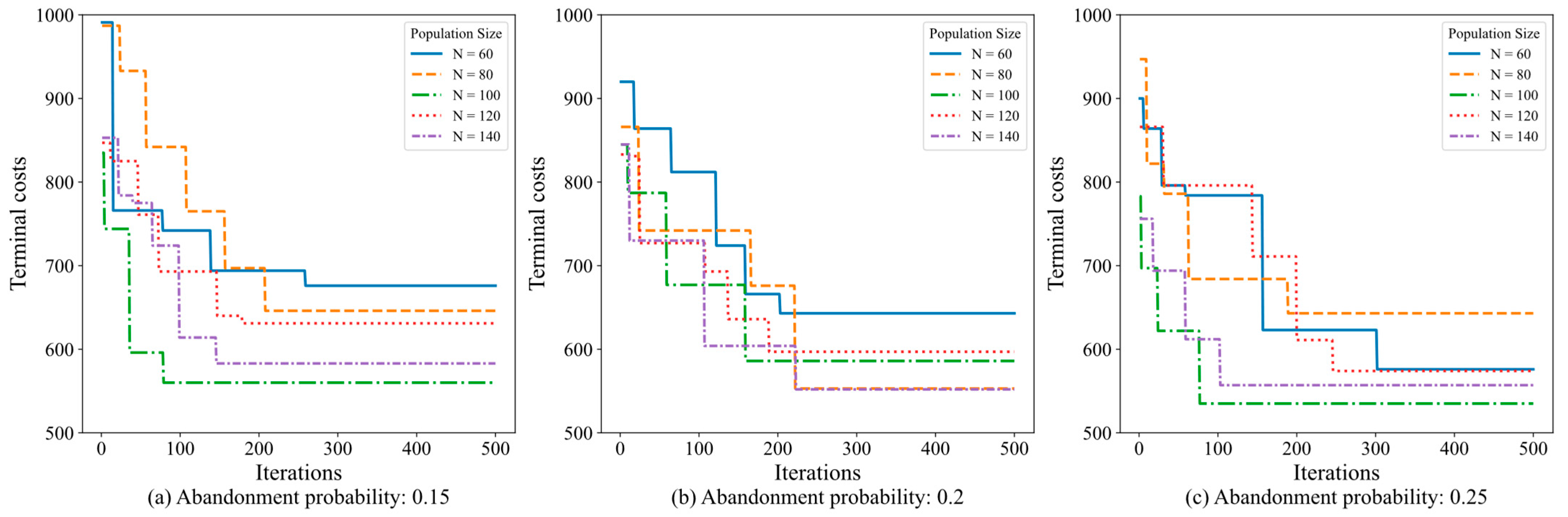
| 0.15 | 461.24 | 503.37 | 522.28 | 660.90 | 853.93 |
| 0.20 | 480.20 | 557.38 | 544.78 | 636.45 | 846.06 |
| 0.25 | 527.75 | 543.71 | 535.50 | 681.12 | 865.78 |
| Vessel | Instance | GUROBI | IMOCS | ||||||
|---|---|---|---|---|---|---|---|---|---|
| Obj1 | Obj2 | T(s) | Obj1 | Gap1 | Obj2 | Gap2 | T(s) | ||
| 10 | 10-1 | 0.00 | 56.10 | 14.35 | 0.00 | 0.00% | 56.10 | 0.00% | 9.66 |
| 10-2 | 0.38 | 66.70 | 16.08 | 0.38 | 0.00% | 66.80 | 0.15% | 6.27 | |
| 10-3 | 0.00 | 64.70 | 12.75 | 0.00 | 0.00% | 64.70 | 0.00% | 6.91 | |
| 10-4 | 0.00 | 54.90 | 13.40 | 0.00 | 0.00% | 54.90 | 0.00% | 10.67 | |
| 10-5 | 0.00 | 68.50 | 16.66 | 0.00 | 0.00% | 68.50 | 0.00% | 8.19 | |
| 15 | 15-1 | 2.12 | 93.38 | 327.44 | 2.14 | 0.94% | 94.48 | 1.18% | 68.91 |
| 15-2 | 6.09 | 77.01 | 569.04 | 6.16 | 1.15% | 77.82 | 1.05% | 99.83 | |
| 15-3 | 8.72 | 81.00 | 201.48 | 8.77 | 0.57% | 81.29 | 0.36% | 81.95 | |
| 15-4 | 10.55 | 86.59 | 222.40 | 10.59 | 0.38% | 87.10 | 0.59% | 76.75 | |
| 15-5 | 7.08 | 84.39 | 757.28 | 7.21 | 1.84% | 85.12 | 0.87% | 81.41 | |
| 20 | 20-1 | 14.09 | 115.69 | 4904.74 | 15.32 | 8.73% | 118.24 | 2.20% | 128.04 |
| 20-2 | 14.77 | 120.05 | 2372.87 | 15.61 | 5.38% | 125.22 | 4.31% | 137.82 | |
| 20-3 | 14.52 | 129.47 | 4951.24 | 14.83 | 2.14% | 131.80 | 1.80% | 199.66 | |
| 20-4 | - | - | - | 11.83 | - | 153.52 | - | 163.90 | |
| 20-5 | 16.67 | 138.21 | 5772.89 | 17.81 | 6.84% | 141.28 | 2.22% | 153.55 | |
| Vessel | Instance | NSGAII | SPEA2 | MOCS | IMOCS | ||||||||
|---|---|---|---|---|---|---|---|---|---|---|---|---|---|
| Obj1 | Obj2 | T(s) | Obj1 | Obj2 | T(s) | Obj1 | Obj2 | T(s) | Obj1 | Obj2 | T(s) | ||
| 30 | 30-1 | 8.7 | 235.4 | 385.7 | 9.3 | 241.7 | 360.1 | 8.5 | 229.1 | 380.2 | 6.1 | 215.7 | 392.6 |
| 30-2 | 7.6 | 244.1 | 405.9 | 7.4 | 243.6 | 415.2 | 6.6 | 245.6 | 420.3 | 6.2 | 223.7 | 390.5 | |
| 30-3 | 8.6 | 183.9 | 450.2 | 7.2 | 221.7 | 480.8 | 8.6 | 208.5 | 430.1 | 6.9 | 172.4 | 490.1 | |
| 30-4 | 13.5 | 251.8 | 315.2 | 11.8 | 261.7 | 370.5 | 11.3 | 266.0 | 405.3 | 11.2 | 238.2 | 350.9 | |
| 30-5 | 4.4 | 217.7 | 460.1 | 5.8 | 220.1 | 425.5 | 4.3 | 211.0 | 360.9 | 3.7 | 197.8 | 369.7 | |
| 40 | 40-1 | 19.4 | 433.1 | 720.5 | 20.8 | 420.4 | 485.3 | 20.7 | 428.5 | 860.1 | 19.2 | 371.6 | 590.8 |
| 40-2 | 24.6 | 381.8 | 550.9 | 24.7 | 387.9 | 780.1 | 23.2 | 375.4 | 670.2 | 23.7 | 368.1 | 480.2 | |
| 40-3 | 25.7 | 488.6 | 890.6 | 31.3 | 462.5 | 530.4 | 28.4 | 489.4 | 620.8 | 20.6 | 434.0 | 800.6 | |
| 40-4 | 33.5 | 413.1 | 730.3 | 31.3 | 418.9 | 720.9 | 32.6 | 438.8 | 490.2 | 29.7 | 434.7 | 540.8 | |
| 40-5 | 32.1 | 391.0 | 870.2 | 31.3 | 425.3 | 760.8 | 28.9 | 443.5 | 790.9 | 28.3 | 389.8 | 750.5 | |
| 50 | 50-1 | 58.5 | 621.8 | 1124.7 | 56.8 | 647.3 | 708.4 | 57.9 | 594.8 | 1458.9 | 58.3 | 534.8 | 890.5 |
| 50-2 | 50.1 | 532.3 | 843.2 | 45.9 | 550.8 | 679.8 | 47.3 | 587.4 | 1027.6 | 43.3 | 496.2 | 1290.3 | |
| 50-3 | 38.9 | 530.2 | 1550.6 | 35.5 | 525.1 | 1189.3 | 37.5 | 503.6 | 1325.8 | 29.8 | 503.4 | 815.3 | |
| 50-4 | 60.8 | 575.6 | 937.8 | 52.4 | 564.7 | 743.6 | 50.9 | 563.7 | 1364.6 | 50.5 | 541.8 | 1101.9 | |
| 50-5 | 41.9 | 505.1 | 1290.1 | 39.1 | 491.2 | 985.4 | 38.9 | 484.4 | 1412.2 | 38.5 | 478.8 | 865.8 | |
| Average | 28.6 | 400.4 | 768.4 | 27.4 | 405.5 | 642.4 | 27.0 | 404.6 | 801.2 | 25.1 | 373.4 | 674.7 | |
| Vessel | Instance | IGD | HV | ||||||
|---|---|---|---|---|---|---|---|---|---|
| NSGAII | SPEA2 | MOCS | IMOCS | NSGAII | SPEA2 | MOCS | IMOCS | ||
| 30 | 30-1 | 0.25 | 0.36 | 0.24 | 0.15 | 0.67 | 0.56 | 0.73 | 0.92 |
| 30-2 | 0.17 | 0.37 | 0.26 | 0.09 | 0.77 | 0.53 | 0.72 | 0.83 | |
| 30-3 | 0.24 | 0.46 | 0.17 | 0.18 | 0.76 | 0.52 | 0.83 | 0.84 | |
| 30-4 | 0.61 | 0.41 | 0.48 | 0.26 | 0.82 | 0.52 | 0.84 | 0.88 | |
| 30-5 | 0.26 | 0.25 | 0.19 | 0.16 | 0.67 | 0.53 | 0.84 | 0.84 | |
| 40 | 40-1 | 0.36 | 0.34 | 0.35 | 0.15 | 0.56 | 0.38 | 0.55 | 0.64 |
| 40-2 | 0.51 | 0.54 | 0.26 | 0.22 | 0.46 | 0.34 | 0.67 | 0.69 | |
| 40-3 | 0.19 | 0.33 | 0.18 | 0.16 | 0.56 | 0.67 | 0.52 | 0.67 | |
| 40-4 | 0.62 | 0.27 | 0.36 | 0.27 | 0.44 | 0.54 | 0.43 | 0.77 | |
| 40-5 | 0.30 | 0.47 | 0.27 | 0.12 | 0.58 | 0.59 | 0.66 | 0.73 | |
| 50 | 50-1 | 0.61 | 0.52 | 0.42 | 0.23 | 0.31 | 0.39 | 0.51 | 0.64 |
| 50-2 | 0.44 | 0.51 | 0.36 | 0.30 | 0.45 | 0.36 | 0.52 | 0.61 | |
| 50-3 | 0.45 | 0.66 | 0.37 | 0.21 | 0.41 | 0.54 | 0.49 | 0.62 | |
| 50-4 | 0.50 | 0.53 | 0.38 | 0.29 | 0.40 | 0.51 | 0.56 | 0.66 | |
| 50-5 | 0.56 | 0.58 | 0.41 | 0.38 | 0.27 | 0.22 | 0.44 | 0.46 | |
| Average | 0.40 | 0.44 | 0.31 | 0.21 | 0.54 | 0.48 | 0.62 | 0.72 | |
| Vessel | NSGAII | SPEA2 | MOCS | IMOCS | |
|---|---|---|---|---|---|
| 20 | Avg.obj1 | 4.5 | 4.8 | 4.2 | 4.0 |
| Avg.obj2 | 151.2 | 134.8 | 142.9 | 128.4 | |
| Avg.time | 125.2 | 118.4 | 131.0 | 141.8 | |
| 30 | Avg.obj1 | 8.5 | 8.3 | 7.8 | 6.8 |
| Avg.obj2 | 226.5 | 237.7 | 232.0 | 209.5 | |
| Avg.time | 268.7 | 289.3 | 320.4 | 303.4 | |
| 40 | Avg.obj1 | 17.1 | 17.8 | 16.7 | 14.3 |
| Avg.obj2 | 421.5 | 423.0 | 435.1 | 399.6 | |
| Avg.time | 752.5 | 655.5 | 686.4 | 632.5 | |
| 50 | Avg.obj1 | 40.2 | 35.9 | 36.5 | 34.1 |
| Avg.obj2 | 553.0 | 555.8 | 546.7 | 511.2 | |
| Avg.time | 1149.2 | 861.3 | 1317.8 | 992.7 |
| Vessel | Instance | Single-Objective () | Single-Objective () | Single-Objective () | Bi-Objective (Min Obj1) | Bi-Objective (Min Obj2) | |||||
|---|---|---|---|---|---|---|---|---|---|---|---|
| Obj1 | Obj2 | Obj1 | Obj2 | Obj1 | Obj2 | Obj1 | Obj2 | Obj1 | Obj2 | ||
| 30 | 30-1 | 13.6 | 209.6 | 9.7 | 246.5 | 5.6 | 298.1 | 6.1 | 277.3 | 13.2 | 215.7 |
| 30-2 | 17.8 | 205.1 | 11.5 | 253.2 | 5.7 | 303.9 | 6.2 | 282.7 | 16.8 | 223.7 | |
| 30-3 | 14.0 | 164.7 | 10.2 | 203.5 | 6.4 | 253.1 | 6.9 | 235.6 | 13.4 | 172.4 | |
| 30-4 | 22.4 | 224.5 | 16.5 | 265.9 | 10.4 | 315.5 | 11.2 | 293.6 | 21.5 | 238.2 | |
| 30-5 | 10.2 | 185.8 | 6.7 | 229.4 | 3.4 | 280.6 | 3.7 | 261.0 | 9.6 | 197.8 | |
| 40 | 40-1 | 26.9 | 344.6 | 21.7 | 401.8 | 18.8 | 464.4 | 19.2 | 432.0 | 24.2 | 371.6 |
| 40-2 | 34.9 | 354.9 | 26.4 | 395.7 | 21.2 | 454.9 | 23.7 | 423.2 | 33.1 | 368.1 | |
| 40-3 | 27.2 | 403.3 | 23.4 | 462.5 | 19.1 | 527.7 | 20.6 | 490.9 | 26.1 | 434.0 | |
| 40-4 | 41.9 | 412.7 | 34.0 | 467.1 | 27.5 | 536.7 | 29.7 | 499.5 | 38.2 | 434.7 | |
| 40-5 | 38.1 | 371.3 | 32.6 | 421.5 | 26.2 | 486.6 | 28.3 | 453.1 | 36.9 | 389.8 | |
| 50 | 50-1 | 70.4 | 516.3 | 61.4 | 559.2 | 57.0 | 627.2 | 58.3 | 583.6 | 64.5 | 534.8 |
| 50-2 | 58.3 | 460.1 | 47.3 | 525.2 | 41.1 | 595.7 | 43.3 | 554.1 | 51.2 | 496.2 | |
| 50-3 | 41.5 | 472.1 | 33.2 | 531.2 | 27.6 | 601.1 | 29.8 | 559.0 | 36.6 | 503.4 | |
| 50-4 | 68.1 | 519.0 | 55.2 | 571.5 | 48.7 | 647.3 | 50.5 | 602.1 | 59.8 | 541.8 | |
| 50-5 | 50.8 | 455.1 | 41.4 | 506.6 | 37.6 | 574.4 | 38.5 | 534.3 | 44.3 | 478.8 | |
| Average | 35.7 | 353.3 | 28.7 | 402.7 | 23.8 | 464.5 | 25.1 | 432.1 | 32.6 | 373.4 | |
Disclaimer/Publisher’s Note: The statements, opinions and data contained in all publications are solely those of the individual author(s) and contributor(s) and not of MDPI and/or the editor(s). MDPI and/or the editor(s) disclaim responsibility for any injury to people or property resulting from any ideas, methods, instructions or products referred to in the content. |
© 2025 by the authors. Licensee MDPI, Basel, Switzerland. This article is an open access article distributed under the terms and conditions of the Creative Commons Attribution (CC BY) license (https://creativecommons.org/licenses/by/4.0/).
Share and Cite
Zhang, X.; Liu, Z.; Zhang, J.; Zeng, Y.; Fan, C. Bi-Objective Optimization for Joint Time-Invariant Allocation of Berths and Quay Cranes. Appl. Sci. 2025, 15, 3035. https://doi.org/10.3390/app15063035
Zhang X, Liu Z, Zhang J, Zeng Y, Fan C. Bi-Objective Optimization for Joint Time-Invariant Allocation of Berths and Quay Cranes. Applied Sciences. 2025; 15(6):3035. https://doi.org/10.3390/app15063035
Chicago/Turabian StyleZhang, Xiaomei, Ziang Liu, Jialiang Zhang, Yuhang Zeng, and Chuannian Fan. 2025. "Bi-Objective Optimization for Joint Time-Invariant Allocation of Berths and Quay Cranes" Applied Sciences 15, no. 6: 3035. https://doi.org/10.3390/app15063035
APA StyleZhang, X., Liu, Z., Zhang, J., Zeng, Y., & Fan, C. (2025). Bi-Objective Optimization for Joint Time-Invariant Allocation of Berths and Quay Cranes. Applied Sciences, 15(6), 3035. https://doi.org/10.3390/app15063035