Abstract
Almost a century ago, the first industrial controllers were introduced to the market, labeled as automatic reset and later generalized to hyper-reset or pre-act. Recently, it has been shown that such control solutions can be characterized as model-based solutions with a simplified disturbance observer developed for an integrating model. The aforementioned controllers, albeit under the name of proportional–integral–derivative (PID) controllers, are still the most commonly used control solutions in practice. With the help of a new interpretation, however, it can be shown that PID controllers are also very well suited for controlling processes with complex non-linear dynamics. This paper investigates the design and feasibility of a family of gain-scheduling controllers for saturated non-linear systems described by a first-order differential equation. It is shown that the process can be linearized either by using locally applicable linear models or by using more narrowly applicable ultralocal models. By combining both approaches, an innovative linearization method around the steady states of the process input and output is proposed. This novel approach emphasizes that the entire process input signal has to be constructed by adding the control increment calculated by the linearization to the value of the considered operating point. Thus, it avoids the uncertainties of those methods, which are based on achieving the actual controller output by integrating the calculated differential values. Another advantage of model-based design is that the saturation of the control signal is included in the design from the outset. Therefore, the undesired integration (windup), which is typical for controllers with explicit integral action, is prevented. The proposed design is illustrated using the control of a liquid tank with variable cross-section as a function of the liquid level. The model-based approach is also used in the evaluation of the transients, where homogeneous responses were obtained over the whole range of process output values. Responses were more homogeneous when simple ultralocal models were used, regardless of controller saturation constraints. Finally, all important innovative aspects of the design are highlighted by a comparison with gain-scheduled PI controller design based on velocity implementation.
1. Introduction
Proportional–integral–derivative (PID) controllers are the most frequently used solutions in the field of process control. However, the proclaimed wide application is only one side of the coin, and the reality is much more complex. This article shows that the effectiveness and efficiency of their design, including application to non-linear processes, can be increased by using long-forgotten historical solutions with automatic reset. And from them the path also opens up to current model-based solutions, which form the basis of modern and postmodern automatic control methods. In search of optimal solutions, it is necessary to question seemingly fixed basic beliefs in current approaches, namely with respect to the associated terminology, the use of an explicit integral action, and the linearization of the (usually) non-linear processes. The rest of the discussion, which attempts to explain the overall context as simply as possible without oversimplifying, is used to point out some long-overlooked important aspects. As a result, PID regulation is presented in a new light and the often-mentioned gap between theory and practice is narrowed.
1.1. The Integral Action Versus Automatic Reset
The first of the widely accepted beliefs concerns the use of integral action as one of the pillars of process control. For a long time, controllers were represented by the so-called series PI and PID controllers, which have their origin in a pneumatic controller dating from the beginning of the 20th century until the Second World War [1,2,3]. However, despite the name PI(D), they did not contain any explicit integrators. This is an important aspect that we will discuss in more detail later. At the heart of the pneumatic structure was a flap–nozzle system, which was a high-gain non-linear amplifier initially used for on-off control. By introducing negative feedback through the lower flexible bellows in Figure 1 with a negligible input resistance, the proportional zone was significantly increased and thus the proportional gain was significantly reduced. The transfer function between the controller input and the output became
The negative feedback not only reduced the excessive gain of the controller, but also linearized the input–output (I/O) characteristics of the controller in the proportional band. The reduced controller gain also eliminated permanent oscillations around the setpoint. The reduced controller gain increased the permanent control error. In order to manually eliminate the steady-state error , the controller output was therefore supplemented with an offset signal (), according to . The ingenious solution was to introduce positive feedback from the controller output using the upper bellows in Figure 1 with the input resistor (valve) , which, together with its capacitance, formed a low-pass filter with a time constant . This eliminated the permanent control error. If the transfer function of the stabilizing controller (1) is supplemented by the positive feedback
you obtain a controller with parallel integral action with the time constant in the proportional band of the control:
The automatic change of the offset was called “automatic reset” and the time constant was called “integral”, although physically it is a filter time constant. By adding the resistor to the negative feedback of the lower bellows with the capacitance , it was finally possible to extend the controller and obtain a proportional–derivative controller with a time constant
In combination with the upper bellows, i.e., with (75), the (series) proportional–integral–derivative controller, which provides the transfer function in the proportional domain of the control, was thus introduced around 1938. The integral action could be switched off by closing the pneumatic resistor (). To switch off the derivative action, it was necessary to open the valve completely (). Since the time constant of the derivative filter was not explicitly set by the users, it seemed quite natural to omit it in the user manuals, and so the “textbook” description of series controllers with the transfer function
became conventional. To summarize, by using feedback in combination with a controller offset fed by low-pass filters from the controller output, it was possible to establish the so-called “integral action” which can compensate not only for external disturbances but also for imperfections in the process model used, known as “internal” disturbances. The integral action has become one of the pillars of process control due to internal feedback [4]. However, the imprecise terminology of integral action has had an impact on the future development of the scientific or engineering discipline discussed. Today’s PID controller aims to equal to the historical pneumatic solution only in the area of proportional control. The early solutions were gradually forgotten and the development of automatic control went in a different direction than could have been expected in the early stages. The textbook and industrial PID controllers are therefore not equivalent, which can be seen as one of the reasons for the often-mentioned gap between theory and practice. As already commented in the conference paper [5], it seems that research related to the linearization of non-linear processes has also contributed to this misunderstanding by searching for the point at which the integrator should be placed into the non-linear controller [6]. The loss of controller effectiveness when using an explicit integrator will be examined in more detail later when discussing process linearization.
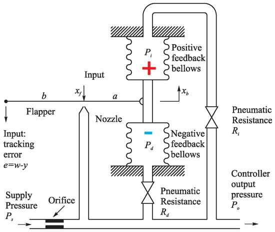
Figure 1.
Pneumatic hyper-reset (series PID) controller.
1.2. Directions of Further Development
The early pneumatic controllers with automatic reset and hyper-reset (ARCs) were later replaced by controllers based on transistors or operational amplifiers. As they merely copied earlier pneumatic controllers, the designation of ARCs with the generic term series proportional–integral–derivative (PID) control did not cause any major problems [7]. However, even in the early days of PID control, there were some misunderstandings, including in connection with the different control structures. For example, the tuning rules of [8] were published for the series controller form and not for the parallel PIDs with an “ideal” transfer function
The designation of both controller types with almost the same name often leads to some authors forgetting to convert the parameters of series (5) to the parallel (6) controller or vice versa. In order to obtain the same transfer function, the parameters of the series and parallel PID controllers (denoted by the indices “s” and “p”) cannot be identical (see, e.g., [9,10]). They must be recalculated according to the following relationships:
Parallel PIDs appeared mainly after the advent of digital computers, which made it possible to realize the integration operation with a simple summation performed with a relatively short sampling period. Recalculation (7), which can only be performed for , shows that the full range of transients that can be adjusted with parallel controllers cannot be achieved by using series controllers. Therefore, the use of parallel PIDs might seem advantageous, even if we disregard the lower production costs of truly digital solutions. However, one of the biggest disadvantages of parallel controllers is the possible uncontrolled integration of parallel PIDs after the control limits are reached (where the series controllers become simple on-off controllers). The parallel controller also does not offer as simple a disturbance reconstruction as the series controller, where it is simply calculated by comparing an expected (estimated) process input with the measured controller output.
Extensive research in the field of anti-windup solutions [7,9,11], which aim to prevent undesirable integration outside the proportional control band, took place during the period of dominance of linear automatic control theory under the two-stage design paradigm. This aims to design the linear controller that neglects the non-linearities of the control signal and then adds anti-windup compensation to minimize the negative effects of any control constraints on the closed-loop performance [12]. It seems that solutions based on the conditioning technique method [13,14] are successful in achieving anti-windup protection because the implicit realization of the controller is similar to the form of the series controller. However, for higher-order (HO) PIDs and HO ARCs, some other solutions [15,16,17] could provide better overall closed-loop results for saturated systems. It is worth mentioning that the HO ARCs are also easy to realize, which further narrows the gap between theory and practice. The advantages of HO ARCs have also been demonstrated in the design of a non-overshooting control system. All the mentioned advantages of HO ARCs have also motivated us to apply them to non-linear processes by using gain scheduling [5].
1.3. Modern and Postmodern Model-Based Control
Let us recall at the outset that, in addition to the search for new innovative solutions, an important task of research is also the consistent analysis and mapping of solutions used so far. Not only in order to effectively extend their effective lifespan and usage [18], but also with the aim to search for new inspiring applications and modifications [19]. Before we turn to non-linear processes, let us return to the specificity of integral action in process control [4]. The expansion of digital control led to a simplification of parallel PID control implementation (e.g., through the transfer function of parallel PID (6)), which seemed to be easier than writing algorithms for the series feedback structure (ARCs). The use of computer simulations and search optimization (such as in [20]) gradually became widespread. The literature contains a myriad list of different approaches to controller tuning, with increasingly exotic and often bio-inspired names [21,22,23,24]. From a research perspective, random search algorithms using artificial intelligence seem to be more attractive than analytical derivations of optimal controller parameters. However, shifting the focus to the advanced optimization algorithms leads to a poorer understanding of the controller structure. In the 1960s, modern control theory (MCT) promised innovative solutions in the field of controller design using a state-space approach to controller design by the pole assignment/placement method and the design of an observer of states and process disturbances [25,26,27,28]. In systems without dead time, MCT can also be successfully used for the analysis and design of ARCs. If it turns out that the structure of ARCs has evolved from the requirement of reconstruction and compensation of disturbances of first-order integral systems [29,30], let us look at this problem from a somewhat generalized point of view. Consider processes whose output and input are described by the Laplace transformation with the first-order model
The basic state space controller is then reduced to a proportional (P) controller with the gain (1) [31] (Figure 2). The additional offset generated by a static feed-forward provides a steady-state error of zero for the piecewise constant setpoints w being considered. Using a first-order disturbance model for piecewise constant input disturbances [25,27,32], one has to use the second-order extended state vector reconstructed by an extended state observer (ESO) [31]. Subsequently, the state space design based on the identical state observer introduces use of second-order filters. Thereby, it provides both the reconstruction and stabilization of the process output, as well as the reconstruction and compensation of constant disturbances. The ESO design and the disturbance reconstruction can be simplified to Figure 2 considering just the filtered reconstructed disturbance described by transfer functions
If the estimation of a piecewise constant disturbance is required with first-order filters, a reduced-order observer can be used. But its design is more complicated [27,28]. The need for filtering came also from the need to work with proper transfer functions (implementability requirement) and from the requirement to prevent the low-pass filter from creating an algebraic loop after introducing disturbance compensation.Since when reconstructing the input disturbance from the process output, must always contain the inverse of the process transfer function (8), and the reconstruction of the filtered disturbance can be proposed in a simplified manner for any integer within the framework of disturbance observer-based control (DOBC) [33,34,35]), even without reconstructing the process state. Moreover, let us recall once again that MCT was initially limited to analog implementation and therefore, just like PID, primarily focused on control design methods not requiring use of dead-time models. Although the “user manual” for PID controllers [8] also allowed for dead time in the controlled time-delayed processes.
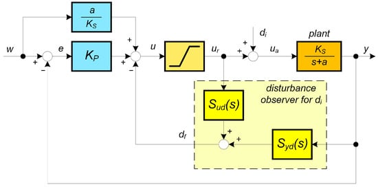
Figure 2.
P-controller for the process with the gain , static setpoint feed-forward and transfer function based disturbance observer (DOB) yielding filtered reconstruction of the input disturbance .
This deficiency regarding dead time was later removed using the internal model control (IMC) approach, which led to a simplification of the reconstruction of output disturbances using a parallel process model [36]. It can be considered a generalization of Smith’s predictor, representing the most famous approach to dead-time compensation [37]. However, simple reconstruction and compensation of disturbances brought about by IMC was only directly possible for stable processes. For integrating process models, the output disturbance is not observable, and for unstable processes, one has to focus on the reconstruction and compensation of the input disturbances [38]. The corresponding structures usually require a significantly more complex design [39,40]. In comparison with the ESO-based control proposed in the MCT framework, which also allows for a simple modification for ultralocal systems with , it was a handicap. This approach is now predominantly used in active disturbance rejection control (ADRC) [32,41,42,43,44,45,46,47].
Both the reconstruction of the output disturbance in the IMC framework and the reconstruction of the input disturbance in the MCT and ADRC framework are based on a comparison of the measured process outputs with their expected values obtained using the process model. Similarly, also in the disturbance observer-based control (DOBC) introduced in [33,34,35], the input disturbance can be reconstructed by comparing the output of the controller with the reconstructed input of the process using the inverse process model. As in (9), both signals should be filtered with the same filter. When disturbance observers (DOBs) use the limited control signal, there is no degradation in control performance compared to the undesired integration (windup) of parallel PIDs without proper anti-windup protection. In the nominal case, the addition of reconstruction and disturbance compensation does not change the dynamics of setpoint tracking provided by the stabilizing controller .
The design of a reduced observer with the value is simpler to explain using the inverse transfer function of the process within the DOBC than in MCT. It also allows for a more flexible choice of with respect to the existing measurement noise. However, it should yet be noted that neither MCT, IMC, nor DOBC mention that the first AR-based controllers used a simplified DOB, which is also effective for non-linear processes with control saturation [16]. This not well-known fact represents one of the main advantages of ARCs compared to heuristic PID controllers. It is not mentioned even in recent publications dealing with DOBC (see, e.g., [48]). On the other hand, when comparing ARCs with DOBC, MTC and ADRC, one should also mention their disadvantage, which is a consequence of using a simplified DOB and which, after introducing disturbance compensation, requires a recalculation of the stabilizing controller. The disturbance compensation in DOBC, MTC, and ADRC in the nominal case does not affect the dynamics of setpoint tracking—it is independent of the setting of the nominal DOB. Therefore, in order to obtain a broader overview of the advantages of individual solutions, it is also important to compare them in the control of non-linear processes. Thereby, the setting of individual linear controllers based on the linearization of the non-linear process around a suitably chosen operating point can usually no longer be considered a nominal case. In this context, another question arises regarding the choice of the linear model used: “local” with in a process linearization (8), or “ultralocal” model with ? Similarly, one can ask about the sensitivity of particular solutions to measurement noise [5]. By choosing the simplest option in (9) with the model parameters and , and considering zero- or first-order polynomials in the numerator of in (9) that produce ARCs, or DOBs, it is possible to introduce and examine four different options for controller design (see Figure 2). Both the local () and the ultralocal () model can be used for the following:
- The design of the stabilizing controller gain ;
- The analysis of stability limits of ;
- The design of the DOBs or ARCs with the filter time constant ;
- The analysis of stable parameters of the loops extended by ARCs and DOBs;
- The robustness analysis of the loops with stabilizing controller and with DOBs or ARCs.
1.4. Process Modeling and Gain-Scheduled Control
The linearization of non-linear processes in order to obtain a linear model that simplifies the calculation of the controller has been a research topic for many decades. It was already mentioned in one of the first textbooks on automatic control by Oldenbourg and Sartorius [49]. In the meantime, numerous general approaches to non-linear systems have been proposed—see, e.g., [50,51,52], textbooks on differential geometric [53] or algebraic methods [54]. The latter led to the introduction of generalized transfer functions for non-linear systems [55,56]. After the introduction of digital controllers, a large number of solutions for the design of non-linear controls became possible. The solutions focused on increasing control performance and robustness by appropriately adapting the controller adjustment, denoted as gain scheduling [6,50,57,58,59,60,61,62,63].
However, a less optimistic view of the problem of controlling non-linear systems results from the IFAC review of the basic methods required for use in industry [64]. And very similar results were provided by the IFAC survey focused on what to teach in the basics of automatic control in the bachelor’s degree. From the point of view of control engineers, who should now also be experts in the field of programming the proposed gain-scheduling controllers, their general characteristics may be given as “too complex”. The effort to be as general as possible could also be the reason that the available works frequently do not proceed from simple to more complex examples, but sometimes even forget to include simple illustrative examples at all. Moreover, when linearizing the process, these works always tried to make full use of the possibility of linearization by deriving the partial derivatives of a non-linear model according to all process variables, although linearization depending on the output of the process (and its derivatives) does not always lead to more accurate control results. Today, the fact that these works were created at a time of dominance of general approaches, dominance of integral action, and dominance of linear control, which from the point of view of saturated design, does not represent the superior option, also appears to be a disadvantage. The possibility of violation of the aforementioned dogmas of the standard controller design procedures used is apparent precisely in these contexts. Their overcoming lies in the possibilities of using ARCs and DOBs based on two types of linear models denoted as “local” and “ultralocal”. This moment brings a new additional degree of freedom to the controller design, used up to now (but just partially) in ADRC and MFC based on ultralocal models. However, this use does not yet fully exploit the overall potential of the generalized linearization methodology, which should not repeat the previous mistakes and limitations, and be presented as simple as possible. The use of PID controller design derived for integral (ultralocal) models also to control processes with a more general model, as used by [65], is far from exceptional. However, a more precise justification for the use of such procedures and the conditions required for their success are lacking.
As the main contributions of this work can be stressed, the consistent model-based design of disturbance reconstruction and compensation closely respecting the essence of historical industrial controllers, the innovative interpretation of process linearization including also the non-linear offset required in transition from calculated control increments to real controller output, and a practical evaluation of the responses performed on a simple illustrative example using performance measures corresponding to the requirements specified in the controller design.
With the aim of providing a practical demonstration of the saturated controller design formulated with respect to the essence of automatic reset-based controllers and applied to first-order non-linear processes, the remainder of this paper, which significantly extends the basic ideas from the conference paper [5], is outlined as follows. Section 2 describes the gain-scheduled model-based constrained controller design exploiting DOBs using inverse (linearized) process models and their simplified versions corresponding to ARCs. Four basic controller versions were proposed on the basis of two basic process linearization options and two basic disturbance observer types. An illustrative example of a non-linear liquid tank with variable cross-section is given in Section 3, where all four non-linear controllers were tested. The unconstrained and constrained controllers were tested. The benefits of the innovative design are highlighted by comparing its outputs with traditional gain-scheduled PI control based on velocity implementation. The evaluation of the captured transients is conducted by quantifying them through modified performance measures that represent deviations of the process output and input from transients with a specified number of monotonic segments. Some concluding remarks, including the novel contributions of the paper, are summarized in Section 4.
2. Generalized Constrained Non-Linear Controller Design
Consider a non-linear system with the input u and the output y
where , and f is a function differentiable with respect to both variables. Since according to the Taylor series expansion
for small increments
around a stationary operating point
satisfying
the system can be linearized as follows:
For sufficiently small deviations (12) from X, if
after application of Laplace transform, linearization (16) of the system (10) can be characterized by a transfer function
This is defined for deviations from the operating point (12). Hence, the operating point symbol X is omitted for the sake of simplicity, and in the control diagrams in Figure 3 the non-linear process (10) can be replaced by the transfer function (17).
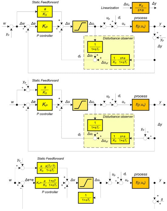
Figure 3.
Proportional controller with a static feed-forward and DOB based on linearization of non-linear process (10) around the operating point ) (13) (above), the alternative scheme with shifted summation points (middle), and the implementation using possibly automatic- or hyper-reset controllers augmented with the measurement noise (below).
For the given linearization (17), several model-based controller structures are considered in [31]. Figure 3 above shows a possible implementation of a whole family of control systems for a non-linear process (10) with the setpoint w and the compensation of unknown piecewise constant disturbances using a disturbance observer (DOB) (9) with . Here, the addition of to the output of the linear controller designed for the linearization of the process around uses the inverse relation to expressed as
This expression of the total control u avoids a possible permanent stationary error of approaches such as [66], where the control signal u is reconstructed by backward integration of the differential . The modification (18) represents an important new solution, as the problems related to the backward integration of the differential control signal can also arise in the rigorous algebraic controller design based on non-linear transfer functions [55]. Furthermore, the need to use non-commutative algebra significantly increases the demands on the analysis and design of the controller.
The need to add the controller offset was already evident in the work of [60]. However, ref. [60] did not yet use multiple ways of process linearization and was not sufficiently distinguished from the usual design of “linear” controllers based on small deviations from the operating point. Offset correction based on the operating point and two basic options for process linearization are also not mentioned in other relevant papers, e.g., [6,61].
2.1. Input Disturbance Reconstruction and Compensation
Using the DOB-based control (DOBC) of the first-order system described by the linearization (17) in the time domain, an input disturbance can be reconstructed as the difference between the actual input to the model and the output of the controller
The implementation requires an additional low-pass filter if the process transfer function is inverted. In the Laplace domain, the signal is calculated from the model output by the filtered process model inversion as follows:
To compensate for the dynamics of the filter in in (19)–(20), the same filter must also be applied to the output of the controller , which provides a filtered reconstructed disturbance in analogy to (9)
With a process model time constant, which is defined as
can be calculated as follows:
Since , with compensation of the control signal increments then correspond to
Here, represents the saturation of the previous control, which was performed with the limit values as follows:
For , the inversion of the process dynamics required to reconstruct the actual input of the model leads to a higher amplification of the measurement noise , as shown in Figure 3 below.
2.2. Selection of the Gain-Scheduling Parameter
The first simplification of the controller can be achieved by selecting the stationary operating point X for the linearization of the process equations. The analysis carried out in [5] has shown that advantageous results can already be achieved by the choice of the scheduling parameter
which results in
and makes it possible to skip the feed-forward path of the controller in Figure 3 below. The choice of a more complex scheduling parameter in [5] did not lead to a significant improvement in performance. For , the stabilizing controller can be modified to the hyper-reset form
In the proportional band of the controller, the positive ARC-like feedback with the time constant enables the PID-like controller transfer function
By considering the model with (resulting in a ) and (stabilized with a ) and zero or the first-degree polynomials in the numerator of in (21), it is possible to derive four different controller options. Since the simplest processes prevail in practice, the first-order non-linear processes (10) are considered when testing the above four options for the model-based gain scheduling controllers. The control design options considered are thus the two types of process model in combination with two types of disturbance observer. To distinguish between them, the corresponding controller parameters will be labeled by subscripts, and the transfer functions will be denoted by superscripts. Their first digits 0 and 1 correspond to the ultralocal and local models, respectively. The second subscript, or superscript, denotes the derivative degree (0 or 1) of the DOB numerator transfer function (9).
2.3. Gain-Scheduled GS-ARC0 Based on Ultralocal Models
For the “nominal” ultralocal model , the controller is based on the parameters , , and . For the stabilizing controller gain and without DOB, it yields a characteristic polynomial
The closed-loop pole corresponds to a time constant of the closed loop . To distinguish two linear models and four possible conditions, they are denoted as and , where
It is often sufficient to reconstruct the disturbance to remove a permanent control error only around the required steady states. This effect can be achieved by using the controller set to and choosing the value of in (21) to be sufficiently large compared to when . Of course, setting , which corresponds to omitting the linearization according to y in (15)–(17), can reduce the accuracy of the approximation and a similar effect can be expected when assuming . This “trivial option” significantly simplifies both the identification of the model and the overall controller design. Furthermore, it also reduces the influence of the measurement noise (see Figure 3 below). The calculated controller corresponds to the automatic reset controller (series PI) [5]. As
the equivalent disturbance-compensating controller in the proportional zone of the control is equivalent to PI controller
Since ultralocal process models are used, they are expected to be sufficiently accurate only in the narrow neighborhood of the operating point. When using the simplest GS-ARC0, it should therefore be noted that:
- The simplest reconstruction of with is achieved for a sufficiently large , i.e., when approaching the steady-states. The disturbance reconstruction and compensation is reduced to a positive feedback from the saturation non-linearity to the offset of the stabilizing controller;
- The saturation limits when calculating the output from correspond to those of u reduced by the offset (18) added to the controller output, if
- If the output correction by the offset according to (18) is omitted, the controller output with the saturation limit defined for u compensates for an equivalent disturbance . As with ADRC, such a cumulative disturbance can then be referred to as a “lumped” or ”total” disturbance.
- As will be shown below, simplifications based on ultralocal models with can only guarantee stable processes for limited tuning parameters and .
2.4. Stability and Overshoot of GS-ARC0 Controller
When analyzing the stability of the closed loop, which is described with an ultralocal model resulting in the P-controller (32) and the actual value of the process model parameter “a” (17), the characteristic polynomial of the closed-loop results is
The stability condition follows from
For any , the stability is always satisfied if . For unstable systems with , has to be chosen sufficiently small to fulfill
In the proportional band of ARC0 control, the simplified DOB
accomplishing the positive ARC0 feedback with , provides the PI controller transfer function (33). The resulting transfer function of the closed-loop is then given as
with the characteristic polynomial
The stability requirement can now be expressed by the inequality
If the proposed gain scheduling is restricted to systems with , all coefficients of the characteristic polynomial are positive and the system remains stable for arbitrary positive values of and . For unstable systems with , the stability of ARC0 will be fulfilled only for a sufficiently large
The stability limit is the same as for a simple P controller (37). By moving value a along the real axis to the left, the required critical value of decreases, the corresponding gain of the controller (32) increases, and for , the stability limit is reached at
Due to the zero in the numerator of , a certain overshoot in the setpoint step response is expected. The easiest way to eliminate this is to use a pre-filter at the controller input w or with a time constant
2.5. GS-DOB0 Controller Based on Ultralocal Models
For the “nominal” ultralocal linearized model , the use of the disturbance reconstruction according to
is equivalent to a stabilizing controller
By substituting , the disturbance-compensating controller takes the form of the automatic reset (series PI) controller
The closed-loop transfer function becomes
The closed-loop stability is guaranteed for
For stable processes with , the loop remains stable for any positive and . For unstable processes with , the system reaches the stability limit for
Using the more complex DOB (45) and the P controller with , the stability region can be extended compared to (43) (the simplified DOB (38) with ). Since the numerator of is equal to , an overshoot of the setpoint step responses is expected. The easiest way to eliminate such an overshoot is to use a pre-filter
An important practical issue for the GS-DOB0 controller is the effect of measurement noise due to the derivative term in (45). It can be adjusted by changing the gain of the stabilizing controller and the AR filter time constant .
Remark 1
(Attenuation of the measurement noise). The amplification of the noise δ can be estimated by calculating the instantaneous change in the controller output (signals and ) caused by the noise increment δ. From the expressions (33), (45), and (47), the changes in the controller outputs can be calculated as follows:
Obviously, for sufficiently long time constants and , the difference between and can be neglected. However, the use of a more complex DOB may no longer make sense. The relationships (52) also mean that the noise attenuation for ARC0 depends on and for DOB0 on and .
2.6. GS-ARC1 Generalized for Local Model
When considering local (linear) models in which is taken into account both in the process description and in the controller design, the simple stabilizing controller yields the closed-loop pole and the time constant
This relationship can in turn be used to adjust the gain of the stabilizing controller according to the following formula:
Remark 2
(Model-based robustness measure). In the nominal case, the local model parameters used for the controller design are equal to the local model parameters that describe the process. Thus, this setting ensures a stability estimate at any value of according to (54). However, if there is a significant difference between and for some , the controller depends heavily on the process linearization and the obtained controller robustness may be reduced (see, e.g., [67]). On the other hand, if , it is likely that the non-linear process can be described with sufficient precision by both linear models. This can be considered as an indication of a sufficient agreement between the expected and the real control responses even further away from the equilibrium points.
If the choice of satisfies at (motivated by the achievement of smooth transients even with a significant amount of measurement noise), the parameter T of the process model can be neglected. This leads to the following transfer function of the equivalent stabilizing controller:
By considering the positive controller feedback, it yields an automatic reset series PI controller, whose gain is defined by the time constant and the “integral” (i.e., automatic reset) time constant
In the proportional band of the controller, the closed loop dynamics with ARC1 (56) becomes
Due to the numerator , overshooting of the setpoint step responses can occur. It can be removed by using a pre-filter
Remark 3
(GS-ARCs with local and ultralocal models). The design of GS-ARCs using local and ultralocal models leads to formally identical controller Equations (33) and (56). The differences lie in the calculation of the stabilizing controller gains (31) and (54), in their relation to the closed-loop time constants, and in the design of the pre-filters (44) and (58) to eliminate overshoots. When designing the controller for unstable processes, the ARC0 controller using ultralocal models does not automatically guarantee the closed-loop stability.
2.7. Nominal GS-DOB1 Tuning
The transfer function of the equivalent stabilizing controller based on the nominal DOB1 considering can be written as follows:
Taking into account the positive controller feedback, it yields automatic reset (series PI) controller with, whose gain is defined by the time constant (53) and the “integral” time constant in (23)
In the proportional control band, the dynamics of the closed control loop with DOB can be described by the transfer function
The nominal DOB, which is based on a local linear model, guarantees the stability of the loop in the form of small increments around the fixed operating point. For positive time constants used in controller tuning, all denominator coefficients in (57) and (61) are positive, so the corresponding closed-loop system remains stable. However, the tuning of the controller can change the numerator. Due to the numerator , overshooting of the setpoint step responses can occur, which can be removed by using a pre-filter
2.8. Overview of the Design Options Considered
The control design options considered are two types of process models in combination with two types of disturbance observers (Table 1). The parameters of the PI controller (Figure 4), which correspond to the ARCs and DOBs considered with (33), (47), (56), and (60) in the proportional zone of the control, are summarized in Table 2. The parameters are expressed in terms of a closed-loop time constant corresponding to a stabilizing P controller and of a filter time constant used in DOB to reconstruct the input disturbance for the plant model (8). The parameters of the current local model are adjusted according to the setpoint w as the scheduling parameter , which provides .

Table 1.
Controller abbreviations.
Remark 4
(The essence of integral action). Although none of the four solutions considered contains an explicit integrator, the integral action is generated implicitly by compensating for the estimate of the input disturbance, which is computed by comparing the reconstructed input to the process and the output of the controller u (see Figure 2). In the case of ARC0, it is most easily reconstructed based on ultralocal process models (i.e., integral model with ) as the steady-state value of the controller output [29]. When , the steady-state output of the process must also be considered in GS-ARC1 to increase the accuracy of reconstruction.
Remark 5
(Research on GS-ARCs and DOBs). ARCs have been used extensively in industry for almost a century. However, their various applications, which arise from the use of two types of linear models based on generally first-order non-linear processes and utilizing simplified disturbance observers (which reconstruct input disturbances just in steady states), are virtually unknown in the literature. The model-based features of ARCs were overshadowed by the heuristic PID control approaches and were also overlooked and misunderstood by the MCT of the 1960s [25,26,27]. Uncovering the specifics of the applied DOB would be even more difficult in MCT, because reconstructing and compensating for disturbances for the first-order processes based on ESO and an identical state and disturbance observer yields a characteristic second-order polynomial in (9) [31].
This also hides the connection between ARC and ADRC [32,68], the latter being essentially a state-space approach simplified by the formulation for ultralocal models with . For the postmodern IMC, the direct connection with ARCs is not obvious, as the output disturbances of ultralocal (integral) models are unobservable [31]. Reciprocal relationships were also not sufficiently clarified for DOBC when DOB was used as an extension of PI control [69]. Paradoxically, simultaneous application of integral action with DOB could lead to degradation of the resulting loop performance, so it requires careful controller design. If the fundamental aspects of the control of linear systems were not clear, the problem is even more evident in the control of non-linear processes.
3. Illustrative Example
Variable dynamics of the system depending on the output and, respectively, the overall state of the system, is relatively common in practice. In order to avoid many important details of more demanding applications, such as they appear, e.g., in connection with attitude control [70], the included illustrative example considers a hydraulic one-tank system with a variable cross-section (see Figure 5), which is described by the differential equation
The input flow rate is considered a control signal (manipulated variable) and the output flow rate depends on the liquid level h. The parameters and depend on the shape of the container, c on the resistance of the outlet tube. Y and U represent the limit values permissible for the given task.
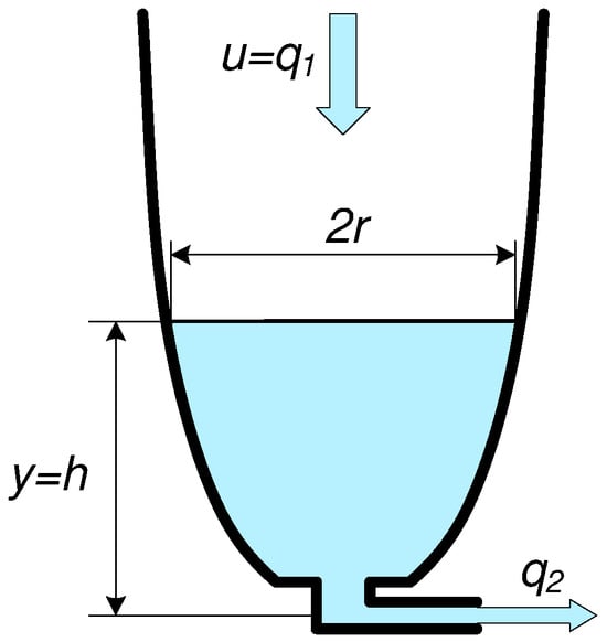
Figure 5.
One-tank hydro system with a variable cross-section.
The results on the application of gain-scheduled PI controllers reported in [71] and supplemented by ARC0 in [5] are now extended by simulating the four options of the model-based control discussed above. Linearization around a steady state (14) with results in a parametrization of the operating point by a single scheduling parameter
The gain-scheduled model
can be specified by the process model (17) as follows:
As mentioned above, there are four possible settings for the controller, depending on the applied model (ultralocal or local, denoted by indices 0 and 1) and the disturbance reconstruction by DOB (with the reconstruction in steady state denoted by 0 or already during transients with 1). The controller settings for the proportional band are calculated from (33), (47), (56), and (60), while the pre-filters are determined from (44), (51), (58), and (62). The main difference from [57] is that only one possible equilibrium state at zero was considered, while now there are infinitely many possible equilibrium states. The works of [6,57,58,59,60,61,62] focused on the control solutions for non-linear systems with multiple inputs and outputs by specifying the position of their poles. On the other hand, a single-input, single-output (SISO) system allows for easy comparison of previously unnoticed differences resulting from two types of linear model and determination of transient uniformity conditions with and without control signal saturation and measurement noise constraints.
To manually adjust the historical analog ARCs, only a constant value was considered when linearizing the system. When control algorithms are implemented with the currently available discrete-time processors, control performance can be significantly increased by adjusting the controller setting separately for each setpoint response based on the gain scheduling parameter (64).
3.1. Preliminary Models and Analysis of the Controller Settings
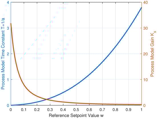
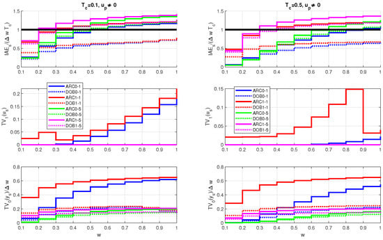
In model-based control, the disturbance can be estimated by comparing the actual system variables with the values calculated from the model. The evaluation of control transients should be performed in a similar way. When using scheduled controllers, the simulated responses should correspond to the selected value of the closed-loop time constant (denoted as for ultralocal models and as for local models). Similarly, the fulfillment of expectations regarding the influence of the DOB time constant can be evaluated. The first test considers controllers with one degree of freedom (1DoF) without control signal limitation. With , the operating range of the process output is defined by the setpoint interval and by the output value . The system model (63) is linearized by the expressions (65)–(66). The resulting linearized process parameters and are shown in Figure 6. Closed-loop responses are analyzed with the scheduling parameter for two sets of tuning parameters given by the combination of two values of with two values of .
The corresponding four sets of equivalent PI controller parameters can be calculated using Table 2. Under the gain-scheduling control with , the parameters and are shown in Figure 7. The values of for the four controllers and the two selections : and depend only on the product . For , controllers with automatic reset (simplified DOB) correspond to ARC0-1 and ARC1-1 and for the full DOB are denoted as DOB0-1 and DOB1-1. For as ARC0-5, ARC1-5, DOB0-5, and DOB1-5.
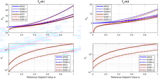
As far as the robustness of the closed loop is concerned, the values of seem to be more interesting. For larger values of w, the values of almost overlap for controllers designed with local and ultralocal models. In contrast, for , the local and ultralocal models yield significantly different settings for . The differences may indicate a lower robustness of the ultralocal models, as already mentioned in Remark 2. The difference between the two values of becomes significantly larger for increased to (with motivation to reduce the output noise of the controller), as shown on the right side of Figure 7. It is therefore clear that the requirements for measurement noise attenuation and the robustness of the closed-loop are contradictory.
3.2. Performance Evaluation for Unconstrained Control
In a detailed comparison of different controller implementations, the input and output signals of the process are evaluated. The speed of the setpoint responses is reciprocal to the integral of the absolute error (), defined as
Since a setpoint response corresponding to a first-order exponential gives the value , the values obtained by simulation are normalized by the time constant (67) and the value according to the relation
For an ideal match with the first-order exponential response given by , the performance measure (69) should give the value 1. Although the use of values may be more useful than other alternative measures [72], the minimum of corresponds to a moderate overshoot. Therefore, it is necessary to avoid such a case by obtaining additional information about the transients of the process output by also considering shape-related measures related to the deviation from monotonicity of the signal.
A response y is monotonic if its total variation () represented by the sum of the absolute values of all increments
corresponds to the total change from an initial value (e.g., ) to a final value . To evaluate the deviation from the monotonicity of the output after a change in the setpoint, the performance measure can therefore be applied [73], which is defined as
Using the values of in relation to the step value , it can be determined that the overshoot percentage () will be less than half of .
The analysis of the process output must be supplemented by the qualitative and quantitative analysis of the process input (controller output). Again, the analysis will be based on modification of the total sum of increments according to
It enumerates summary deviations over two monotonic input intervals, which form a pulse with an extreme point. The first monotonic interval corresponds to the transition from an initial value to the extreme value , which forces the output to follow the new setpoint. The next monotonic segment corresponds to the reduction in the controller output from the extreme value to a stationary value . All increments contributing to can be considered as redundant increments.
3.3. Responses with Unconstrained 1DoF Controllers
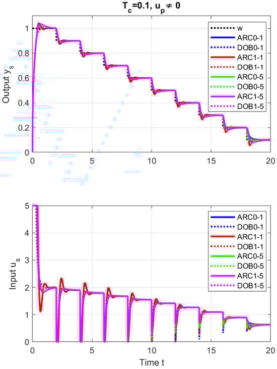
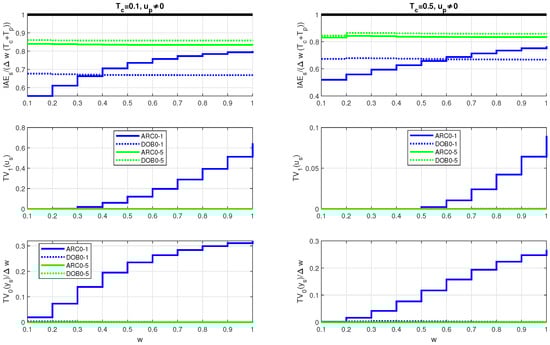
The transients of all four GS controller options, each of them corresponding to ten smaller setpoint steps with , are shown in Figure 8 above. Gradually increasing the setpoint variable through such a sequence of steps allows the gain-scheduled transients with to be checked over a wider range of output values. Each of the closed-loop time constants (67) is associated with two filter time constants . The simplified ARCs are expected to be more effective for increased values of . Consequently, more complex DOBs are also expected to be efficient at smaller values. Obviously, the transients follow the gradually increasing set point quickly for all four controller options. In detail, they can be analyzed using appropriate performance measures in Figure 9 above. Normalized values (69) deviate from the ideal value in virtually all simulations.
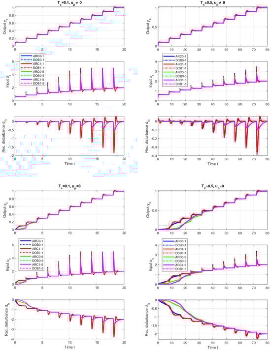
For small values of w, closed-loop responses are faster than should correspond to the value of used for the calculation of . In contrast, closed-loop responses are slower for larger values of w. The values indicate that all the response steps can exhibit a certain overshoot in the output. The evaluation with fast and slow settings of the stabilizing controller , each in combination with two values, thus reveals some interesting facts:
- The corresponding to the local ARC1 models is larger than in the case of the simpler ultralocal ARC0 models.
- If you choose a smaller filter time constant , the overshoots are relatively large when using ARCs, while for they are about the same as when using more complex DOBs.
- Smaller values of for can apparently be achieved with DOBs. But even here, the DOB0s based on the ultralocal model result in less deviations from monotonicity () than the DOB1s.
- With the exception of ARCs, which correspond to , none of the options considered leads to excessive control effort with .
In this evaluation carried out without measurement noise, Figure 9 middle shows excessive controller effort only for ARC0 and ARC1 with fast setting and . For and , only ARC1-1 based on more complex local models gives more excessive controller effort.
3.4. Offset Impact
As can be seen in Figure 3, the actual input of the process depends on the addition of the input disturbance and the offset of the controller (which is part of the total output of the non-linear GS controller (18)). The signal could be formally replaced by the total “lumped disturbance” . The question is whether the reconstruction and compensation of such a lumped disturbance provide the same performance as before.
The transients shown in Figure 8 (down) correspond to GS controllers without using the separate value in (18). They illustrate the advantages of treating the controller offset and disturbance compensation separately for accelerated responses. The omission of the value is particularly evident at lower setpoints and for slower controllers, i.e., when the controller gains based on local and ultralocal models differ significantly, as mentioned in Remark 2. This finding also affects other approaches used for non-linear process, such as the ADRC mentioned earlier.
In contrast to the zero disturbance values reconstructed in the steady states of the upper responses, the lumped values shown below are a replacement for the omitted values of . The differences in Figure 8 above and below also indicate that the rate of convergence of the reconstructed disturbances to the external disturbances will depend on the liquid level. Correction in the GS controllers should be performed after each change in the setpoint. For disturbances with a constant setpoint, the change in is usually not necessary. Therefore, a more detailed qualitative and quantitative analysis of the omission of for disturbance responses (discussed in [5]) is not performed.
3.5. Choice of the Scheduling Parameter and Stability of Transients
By the first experiment with a large step change of the desired output from 0 to 1 and a series of small downward steps in Figure 10, it can be shown that the size of the change in the reference setpoint itself does not significantly affect the shape of the transient responses.
However, destabilizing the circuit by changing the setpoint value w before reaching steady state (Figure 11) has much worse consequences. When using local models ARC1 and DOB1, it leads to a loss of stability at . The conclusion that the use of “more accurate” local models in a non-linear context can lead to unstable, i.e., “less accurate” control results, has been known for several decades (see e.g., the application of local and ultralocal models in [74]).
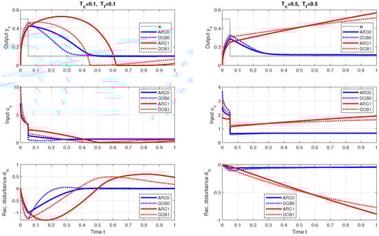
Closed-loop stability analysis when using the controllers ARC0 and DOB0 based on the ultralocal model () shows that they remain stable at arbitrary values , or . Thus, if the sign of the parameter is correctly determined ( does not change its polarity depending on the scheduling parameter), stability does not need to be considered further. This is one of the most important advantages of using ultralocal models. When using local models, the stability of the circuit depends on the settings used, and its analysis usually requires much more attention. In order to keep the length of this article within a reasonable range, we will avoid it in the following text.
3.6. 2DoF Unconstrained Ultralocal Control
All the above responses obtained with a one degree-of-freedom (1DoF) controller do not guarantee homogeneity of values. This problem is a consequence of the zero of the particular closed-loop transfer functions, which may depend on the process linearization parameters, as for example for (57). Thus, the responses are not invariant against the change in the setpoint value. In addition to this fact, they also exhibited non-zero values, indicating a possible overshoot of the output up to . In fact, the responses obtained may be completely satisfactory for most applications. However, to eliminate the overshoot in some critical applications, two-degree-of-freedom (2DoF) controllers with pre-filters can be used. When using local models, the setting of the pre-filters (58) and (62) depends on the parameter and thus also on the scheduling parameter (26) (see Table 2). This increases the complexity of the implementation. Since the 1DoF ARC1 and the DOB1 did not improve performance in the previous experiments and can also cause stability problems due to destabilizing setpoint changes, the evaluation of the 2DoF controllers focuses only on the ARC0 and DOB0 controllers with the pre-filters (44) and (51).
Figure 12 shows the responses based on the fast and slow controllers (with the values and ), using two settings of the disturbance reconstruction filter and , respectively. The quantitative evaluation of the responses in Figure 13 confirms that (with the exception of ARC0 with the value ) the step responses are obtained with zero deviations from the monotonicity of the process output and with zero deviations from the 1P process input signal . These monotonic responses are homogeneous and achieve a slightly smaller value than the sum of the time constants (i.e., ). At the same time, the values achieved do not depend significantly on and almost do not depend on w. For larger values, the normalized values are similar throughout the entire range of the setpoint values w for both controllers considered. This shows that it then makes more sense to use simpler ARCs.
3.7. Impact of the Measurement Noise
To illustrate the effects of measurement noise, a random noise was added to the output y (see Figure 3 below). Noise was generated in the simulation by the “Uniform Random Number” block in Matlab/Simulink with a sampling period . The fluctuations in performance measures caused by noise are mainly visible in the shape-related performance measures, which are represented by the values of and listed in Table 3 and Table 4. In contrast to the performance measures shown in Figure 13, where the shape deviations for DOB0-5 and ARC0-5 were almost zero with the value , the values for DOB0-X are always higher than those for ARC0-X, X = 1,5 under the measurement noise. If you increase the time constants and , both shape deviations are significantly reduced. It is worth mentioning that, for ARC0, the increase in the filter time constant (i.e., from ARC0-1 to ARC0-5) does not lead to a significant reduction in the excessive controller effort compared to DOB0-1 with and DOB0-5 ( of ARC0 controllers does not depend on ). These results obviously show that the choice of the optimal controller depends on the actual circumstances.
Table 3.
Performance measures in the case of measurement noise with amplitude of the Uniform Random Number noise generator and , .
Table 4.
Performance measures in the case of measurement noise with amplitude of the Uniform Random Number noise generator and , .
3.8. Constrained Control
In recent decades, much attention has been devoted to the research of the relationship between traditional and generalized PIDs and postmodern model-based controllers, which is important especially from the point of view of effective control saturation consideration. A collection of such attempts can be well illustrated in the ADRC area, where the problem usually is the higher phase lag due to the second-order ESO filter [42,75,76,77,78]. However, the context of the simpler DOBs design with reduced-order filters, their connection with historical ARCs, and interpretation within the framework of the control of non-linear processes have not yet been sufficiently clarified [46,47,79,80].
The above analysis focused on the compensation of process non-linearities using the local and ultralocal model approximations. The controller parameters were chosen so that homogeneous closed-loop dynamics (in the sense of homogeneous values ) is achieved over the entire range of permissible operating points. In this case, the controller parameters are also selected according to the limitations of the control signal. Due to the saturation constraints, almost constant values of are no longer possible. Instead, we will focus on obtaining homogeneous shapes of the setpoint and disturbance responses at different amplitudes of the setpoint and disturbance steps.
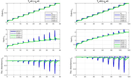
From the responses in Figure 14 and from the corresponding performance measures in Figure 15, it can be seen that the upper limit of the controller output specifies the saturation limits.
The sets of time constants considered are then given as
The corresponding controllers will be denoted as ARC0-1, ARC0-5, ARC0-10, and DOB0-1, DOB0-5, and DOB0-10. For the selected values (74), together with the control constraints (73), the set points are limited in the interval . The shape-related performance measures in Figure 15 show that the requirement for ideal shapes of the input and output signals of the process leads to more constrained responses up to the need to use . This finding complements the analysis of disturbance responses presented in [5]. It showed that the increased time constant in saturated control leads to non-overshooting ARC0 responses while ensuring reconstruction of the disturbance around the steady state. The control constraints prolong the initial saturated phase of the transient responses. Therefore, the time constant must be increased based on the increase in the length of the saturation phase compared to the stabilizing controller without constraints. The value of no longer describes the time constant of the constrained responses in the closed loop and must be increased to a more realistic value.
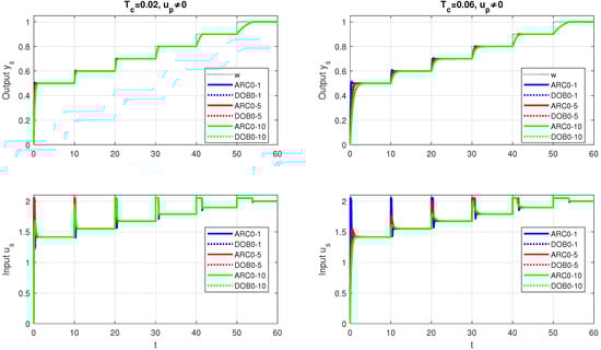
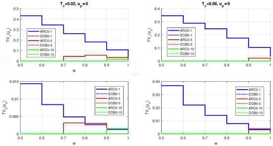
Figure 15.
Performance measures of the constrained setpoint step responses from Figure 14 for (left) and (right); , and : Above—; below—.
If you work with a sufficiently large value , the homogeneity of the shape achieved in step responses also applies to situations where the control does not have saturation. Again, it is obvious that the simplified ARC0 cannot replace the more complex DOB0 for all controller parameter settings, but there are also settings where both types are almost equivalent. Such comparisons are of immense importance for explaining the historical status of both types of controller and for other model-based solutions.
3.9. Comparison with Gain-Scheduled PI Control
Kaminer et al. analyzed in [6] the reasons for a loss of performance or even instability of the feedback system linearized about the operating points and as a solution they proposed velocity implementation of controllers [11,81]. For a fairly general class of solutions that are usually referred to as tracking controllers, differentiating some of the measured outputs before they are fed back to the gain-scheduled controller is applied. Due to the integration of control signal provided at the output of the controllers, despite the use of differentiation, this scheme does not introduce additional noise amplification and allows for relatively easy consideration of control saturation without causing windup. The PI controller with a gain and integral time constant can be defined by the transfer function
With and for a piecewise constant setpoint signal w, the velocity controller implementation can then be described by
For the process (8), application of the PI controller yields the close-loop transfer function
By requiring a double real closed-loop pole , or a time constant , corresponding to the chosen polynomial in (77), the PI parameters can be determined according to
With the scheduling parameter (26), this controller can be scheduled according to (66). Let us recall that the velocity implementation of the PI controller (76) requires the availability of the derivative of the output, which can generally be achieved by using a filter with a derivative time constant according to
However, completely different rules will apply to the optimal setting of the value of than when choosing in controllers with DOB.
As shown by the setpoint step responses and the corresponding performance measures in Figure 16, the gain-scheduled PI controller according to [6] denoted as 1DOF PI1 (red curves) provides good responses with zero shape-related deviations from ideal responses, which are, however, dependent on the magnitude of the setpoint variable w and slower than the responses with 2DoF model-based controllers ARC0-1 and DOB0-1.
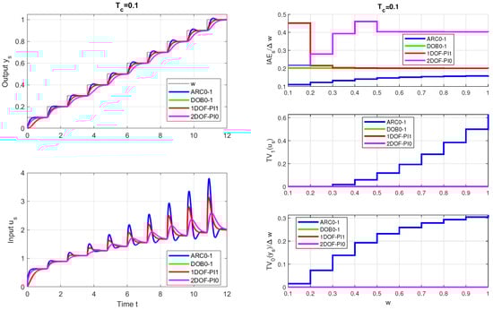
Figure 16.
Setpoint step responses of one-tank hydro system with a variable cross-section (63) with 2DoF gain-scheduled ARC0 and DOB0 controllers, pre-filters (44) and (51), , , gain-scheduled 1DOF PI1 controller according to [6] with and its 2DOF PI0 modification according to (80), (18) (left) and the corresponding performance measures (right).
Remark 6
(Different dynamics requirements of ARC, DOB, and PI controllers). A more detailed analysis of the performance achieved would require noting the differences in the first-order closed-loop dynamics corresponding to gain-scheduled ARC0 and DOB0 controllers with disturbance reconstruction and compensation according to Figure 3 and the second-order dynamics corresponding to the 1DoF PI1 controller with velocity implementation according to (79). While for the ARC0 and DOB0 controllers, the gain is designed from the requirement of the time constant of the first-order exponential (31), for GS-PI according to [6] (1DOF PI1) the controller setting is calculated based on the requirement of double time constant for setpoint tracking. This difference alone indicates that significant differences in the achieved transients can be expected from both solutions.
However, the comparison with the gain-scheduled PI controller according to [6] also opens new topics for further research. Kaminer et al. did not consider the possibility of using two types of linear model—their approach was formulated only using local models. However, considering , this approach can also be reformulated for ultralocal models. They neglected the fact that the linear controller (76) should only be used to calculate small increments of the control signal according to
which are added to the working point (18) (see Figure 17). Kaminer et al. did not consider the possible homogenization of the output dynamics achieved by removing the zero of the transfer function (77) using a pre-filter.
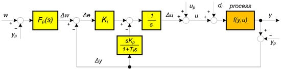
Figure 17.
2DoF velocity implementation of gain-scheduled PI controller with a pre-filter and inverse transformation from to u according to (18).
This can be easily implemented again only for ultralocal models (Figure 17), when the pre-filter time constant is independent of the operating point, whereby it holds
The curves corresponding to the 2DoF PI0 controller are shown in Figure 16 (magenta). The effect of adding to the PI controller output is similar to the changes discussed in Section 3.4 Offset impact. Even this modification of the GS-PI controller does not ensure the high homogeneity of the waveforms achieved with the DOB0-1 controller. For the values, even ARC0-1 gives smaller and more homogeneous values than 1DOF-PI1 or 2DOF-PI0.
The comparison of ARC0 and DOB0 controllers with GS-PI alternatives does not change even when choosing larger values of in Figure 18. None of the modifications considered for GS-PI controllers ensures the homogeneity of values in the entire range of w changes achieved by DOB0-1 and ARC0-1 controllers. The advantage of both 1DOF-PI1 and 2DOF-PI0 is smooth controller output waveforms, which approach ideal shapes. 1DoF-PI1 and 2DoF-PI0 complement each other. The former is suitable for larger values of w, the latter for lower w. However, this only highlights the long-term unrecognized and unused advantages of the solution, whose neglect is closely related to the prevailing interpretations of PID control and process linearization.
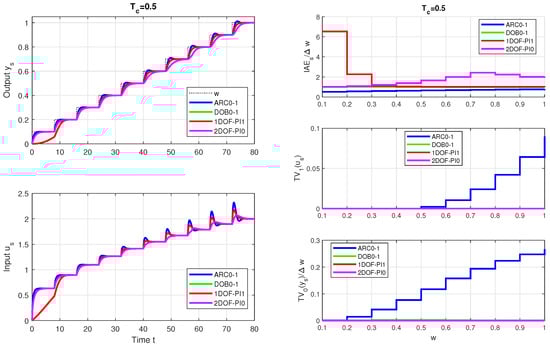
Figure 18.
Setpoint step responses of one-tank hydro system with a variable cross-section (63) with 2DoF gain-scheduled ARC0 and DOB0 controllers, pre-filters (44) and (51), , , gain-scheduled 1DOF PI1 controller according to [6] with and its 2DOF PI0 modification according to (80), (18) (left) and the corresponding performance measures (right).
It would also be interesting to quantitatively compare the thus modified GS-PI controller with the aforementioned ARC and DOB-based controllers, also from the point of view of measurement noise attenuation and saturated control. It may also be interesting to prove and compare the stability and domains of attraction of possible equilibria in such modified gain-scheduled PI controllers and in the above-designed ARCs and DOBs using appropriate methods; for example, Lyapunov functions. However, it is certainly not possible to solve all the open questions that have accumulated over the 9 decades of existence of automatic reset controllers in a single publication.
4. Conclusions
The work took advantage of the recent revelation that official interpretations of PID control do not explain the essence of historical industrial controllers based on automatic reset. A new interpretation of automatic reset controllers considers them as model-based solutions with a simplified disturbance observer designed on the basis of integrative models with first-order dominant dynamics. The work therefore focused on additional study of their use for control of non-linear systems with first-order dominant dynamics. The choice of the objective appropriate to the essence of automatic reset controllers together with a consistent solution of the linearization problem led to the fact that the proposed controllers enable achieving higher performance and higher independence from the choice of the operating point than PID control approaches. These results are interpreted as a consequence of more accurate respect for essential aspects of controlled processes, while PID control is based only on secondary equivalent system properties valid only in a narrow range of transient responses in the proportional control band. This paper also showed that the proposal, which includes four different types of controllers based on two types of linear process models and two types of disturbance observers, also includes other well-known approaches including disturbance observer control (DOBC), modern control theory (MCT), and active disturbance rejection control (ADRC). It also pointed out frequent inconsistencies regarding the linearization of non-linear processes arising from the transition from the calculated increments of the control signal to its total value. In this way, it not only shows the ways to better use different approaches to controlling non-linear processes, but also to better understand their mutual connections. A detailed analysis of four approaches to process linearization and two types of disturbance observers applied to the control design of the considered first-order non-linear system showed the clear advantages of automatic reset-based solutions based on ultralocal models compared to gain-scheduled PI controller design. Their results can be further improved by using full DOB with inversion of the ultralocal model.
In future research, several types of linear models will be developed for more complex non-linear systems with time delays. Controllers with higher-order derivatives are expected to be the most suitable for such models [19,82,83,84,85,86,87,88,89].
Author Contributions
Writing—original draft preparation, M.H.; writing—review and editing, M.H., P.B. and D.V.; simulations, M.H.; project administration, P.B. All authors have read and agreed to the published version of the manuscript.
Funding
This research was supported in part by the following grants: Grant No. 1/0821/25 financed by the Scientific Grant Agency of the Ministry of Education, Research, Development and Youth of the Slovak Republic (VEGA); Grant No. APVV-21-0125 financed by the Slovak Research and Development Agency; Research Program P2-0001 (Systems and Control) and research project L2-3166 (Supervisory control system for plant-wide optimization of wastewater treatment plant operation) financed by the Slovenian Research and Innovation Agency; Grant Agreement No 875047 (project RUBY) financed by Clean Hydrogen Partnership (EU Horizon 2020).
Institutional Review Board Statement
Not applicable.
Informed Consent Statement
Not applicable.
Data Availability Statement
The original contributions presented in this study are included in the article. Further inquiries can be directed to the corresponding author.
Acknowledgments
Supported by E-Academia Slovaca, a non-profit organization, Sadmelijská 1, 831 06 Bratislava, Slovakia. This paper is an extended version of our paper published in Proceeding of the PDES 2024 conference [5].
Conflicts of Interest
The authors declare no conflicts of interest.
Abbreviations
The following abbreviations are used in this manuscript:
| 1P | One-Pulse, response with two monotonic segments (one extreme point) |
| 1DoF | One Degree of Freedom |
| 2DoF | Two Degrees of Freedom |
| AR | Automatic Reset |
| ARC | Automatic Reset Controller |
| ADRC | Active Disturbance Rejection Control |
| DOB | Disturbance Observer |
| DOBC | Disturbance Observer-Based Control |
| ESO | Extended State Observer |
| GS | Gain-Scheduled |
| HO | Higher-Order |
| HO-AR | Higher-Order Automatic Reset |
| Integral of Absolute Error | |
| IMC | Internal Model Control |
| I/O | Input–Output |
| MCT | Modern Control Theory |
| MFC | Model-Free Control |
| P | Proportional |
| PI | Proportional–Integral |
| PID | Proportional–Integral–Derivative |
| SISO | Single-Input Single-Output |
| TV | Total Variation |
| TV0 | Deviation from Monotonicity |
| TV1 | Deviation from 1P Shape |
References
- Bennett, S. Development of the PID controller. Control Syst. IEEE 1993, 13, 58–62. [Google Scholar]
- Bennet, S. A Brief History of Automatic Control. IEEE Control Syst. 1996, 16, 17–25. [Google Scholar]
- Bennett, S. The Past of PID Controllers. In Proceedings of the IFAC Workshop on Digital Control: Past, Present and Future of PID Control, Terrassa, Spain, 5–7 April 2000; IFAC Proceedings Volumes. Volume 33, pp. 1–11. [Google Scholar]
- Skogestad, S. PID is the Future of Advanced Control. In Proceedings of the 4th IFAC Conference on Advances in Proportional-Integral-Derivative Control PID 2024, Almería, Spain, 12–14 June 2024. IFAC-PapersOnLine. [Google Scholar]
- Huba, M.; Bistak, P.; Vrancic, D. Practice-oriented controller design of a simple nonlinear system. In Proceedings of the 18th IFAC Int. Conf. on Programmable Devices and Embedded Systems—PDES 2024, Brno, Czech Republic, 19–21 June 2024. [Google Scholar]
- Kaminer, I.; Pascoal, A.; Khargonekar, P.; Coleman, E. A Velocity Algorithm for the Implementation of Gain-scheduled Controllers. Automatica 1995, 31, 1185–1191. [Google Scholar] [CrossRef]
- Glattfelder, A.; Schaufelberger, W. Control Systems with Input and Output Constraints; Springer: London, UK, 2003. [Google Scholar]
- Ziegler, J.G.; Nichols, N.B. Optimum settings for automatic controllers. Trans. ASME 1942, 64, 759–768. [Google Scholar] [CrossRef]
- Åström, K.J.; Hägglund, T. Advanced PID Control; ISA: Research Triangle Park, NC, USA, 2006. [Google Scholar]
- Huba, M.; Chamraz, S.; Bisták, P.; Vrančić, D. Making the PI and PID Controller Tuning Inspired by Ziegler and Nichols Precise and Reliable. Sensors 2021, 18, 6157. [Google Scholar] [CrossRef]
- Åström, K.J.; Hägglund, T. PID Controllers: Theory, Design, and Tuning, 2nd ed.; Instrument Society of America: Research Triangle Park, NC, USA, 1995. [Google Scholar]
- Kothare, M.V.; Campo, P.J.; Morari, M.; Nett, C.N. A Unified Framework for the Study of Anti-windup Designs. Automatica 1994, 30, 1869–1883. [Google Scholar] [CrossRef]
- Hanus, R.; Kinnaert, M.; Henrotte, J. Conditioning technique, a general anti-windup and bumpless transfer method. Automatica 1987, 23, 729–739. [Google Scholar] [CrossRef]
- Hanus, R.; Peng, Y. Conditioning technique for controllers with time delays. IEEE Trans. Aututomatic Control 1992, 37, 689–692. [Google Scholar] [CrossRef]
- Huba, M.; Vrančić, D.; Bisták, P. PID Control with Higher Order Derivative Degrees for IPDT Plant Models. IEEE Access 2021, 9, 2478–2495. [Google Scholar] [CrossRef]
- Huba, M.; Bistak, P.; Vrancic, D. Series PID Control with Higher-Order Derivatives for Processes Approximated by IPDT Models. IEEE TASE 2024, 21, 4406–4418. [Google Scholar] [CrossRef]
- Huba, M.; Bistak, P.; Vrancic, D. Parametrization and Optimal Tuning of Constrained Series PIDA Controller for IPDT Models. Mathematics 2023, 11, 4229. [Google Scholar] [CrossRef]
- Zhao, D.; Gao, C.; Li, J.; Fu, H.; Ding, D. PID control and PI state estimation for complex networked systems: A survey. Int. J. Syst. Sci. 2025, 1–16. [Google Scholar] [CrossRef]
- Kumar, V.; Hote, Y.V. New approach of series-PID controller design based on modern control theory: Simulations and real-time validation. Ifac J. Syst. Control 2025, 31, 100295. [Google Scholar] [CrossRef]
- Åström, K.J.; Panagopoulos, H.; Hägglund, T. Design of PI Controllers based on Non-Convex Optimization. Automatica 1998, 34, 585–601. [Google Scholar] [CrossRef]
- Kallannan, J.; Baskaran, A.; Dey, N.; Ashour, A. Bio-Inspired Algorithms in PID Controller Optimization; CRC Press: Boca Raton, FL, USA, 2018. [Google Scholar]
- Valluru, S.K.; Singh, M. Optimization Strategy of Bio-Inspired Metaheuristic Algorithms Tuned PID Controller for PMBDC Actuated Robotic Manipulator. Procedia Comput. Sci. 2020, 171, 2040–2049. [Google Scholar] [CrossRef]
- Dutta, P.; Pal, S.; Kumar, A.; Cengiz, K. Artificial Intelligence for Cognitive Modeling: Theory and Practice; Chapman and Hall/CRC: New York, NY, USA, 2023. [Google Scholar]
- Sahoo, A.; Mishra, S.; Acharya, D.; Chakraborty, S.; Swain, S. A comparative evaluation of a set of bio-inspired optimization algorithms for design of two-DOF robust FO-PID controller for magnetic levitation plant. Electr. Eng. 2023, 105, 3033–3054. [Google Scholar] [CrossRef]
- Luenberger, D. Observers for multivariable systems. IEEE Trans. Autom. Control 1966, 11, 190–197. [Google Scholar] [CrossRef]
- Brogan, W.L. Modern Control Theory; Prentice Hall: Upper Saddle River, NJ, USA, 1991. [Google Scholar]
- Ackermann, J. Abtastregelung; Springer: Berlin, Germany, 1988. [Google Scholar]
- Ogata, K. Modern Control Engineering, 5th ed.; Prentice Hall: Upper Saddle River, NJ, USA, 2010. [Google Scholar]
- Huba, M.; Gao, Z. Uncovering Disturbance Observer and Ultra-Local Plant Models in Series PI Controllers. Symmetry 2022, 14, 640. [Google Scholar] [CrossRef]
- Huba, M. Disturbance Observer in PID Controllers for First-Order Time-Delayed Systems. In Proceedings of the 13th IFAC Symposium Advances in Control Education, Hamburg, Germany, 24–27 July 2022. [Google Scholar]
- Huba, M.; Zakova, K.; Bistak, P.; Hypiusova, M.; Tapak, P. Seeking a unique view to control of simple models. IFAC-PapersOnLine 2019, 52, 91–96. [Google Scholar] [CrossRef]
- Gao, Z. On the centrality of disturbance rejection in automatic control. Isa Trans. 2014, 53, 850–857. [Google Scholar] [CrossRef]
- Ohishi, K. A new servo method in mechantronics. Trans. Jpn. Soc. Elect. Eng. 1987, 107-D, 83–86. [Google Scholar]
- Ohishi, K.; Nakao, M.; Ohnishi, K.; Miyachi, K. Microprocessor-Controlled DC Motor for Load-Insensitive Position Servo System. IEEE Trans. Ind. Electron. 1987, IE-34, 44–49. [Google Scholar]
- Sariyildiz, E.; Oboe, R.; Ohnishi, K. Disturbance Observer-Based Robust Control and Its Applications: 35th Anniversary Overview. IEEE Trans. Ind. Electron. 2020, 67, 2042–2053. [Google Scholar] [CrossRef]
- Morari, M.; Zafiriou, E. Robust Process Control; Prentice Hall: Englewood Cliffs, NJ, USA, 1989. [Google Scholar]
- Smith, O. Closser control of loops with dead time. Chem. Eng. Prog. 1957, 53, 217–219. [Google Scholar]
- Huba, M.; Bisták, P.; Vrančić, D.; Zakova, K. Asymmetries in the Disturbance Compensation Methods for the Stable and Unstable First Order Plants. Symmetry 2020, 12, 1595. [Google Scholar] [CrossRef]
- Åström, K.J.; Hang, C.C.; Lim, B.C. A new Smith predictor for controlling a process with an integrator and long dead-time. IEEE Trans. Autom. Control 1994, 39, 343–345. [Google Scholar] [CrossRef]
- Hölzl, S.L. The case for the Smith-Åström predictor. J. Process. Control 2023, 128, 103026. [Google Scholar] [CrossRef]
- Wu, Z.; Gao, Z.; Li, D.; Chen, Y.; Liu, Y. On transitioning from PID to ADRC in thermal power plants. Control. Theory Technol. 2021, 19, 3–18. [Google Scholar] [CrossRef]
- Lin, P.; Wu, Z.; Fei, Z.; Sun, X.M. A Generalized PID Interpretation for High-Order LADRC and Cascade LADRC for Servo Systems. IEEE Trans. Ind. Electron. 2022, 69, 5207–5214. [Google Scholar] [CrossRef]
- Sun, Y.; Su, Z.G.; Sun, L.; Zhao, G. Time-Delay Active Disturbance Rejection Control of Wet Electrostatic Precipitator in Power Plants. IEEE Trans. Autom. Sci. Eng. 2022, 20, 2748–2760. [Google Scholar] [CrossRef]
- Wang, R.; Li, X.; Zhang, J.; Zhang, J.; Li, W.; Liu, Y.; Fu, W.; Ma, X. Speed Control for a Marine Diesel Engine Based on the Combined Linear-Nonlinear Active Disturbance Rejection Control. Math. Probl. Eng. 2018, 2018, 7641862. [Google Scholar] [CrossRef]
- Madonski, R.; Herbst, G.; Stankovic, M. ADRC in output and error form: Connection, equivalence, performance. Control Theory Technol. 2023, 21, 56–71. [Google Scholar] [CrossRef]
- Stankovic, M.; Ting, H.; Madonski, R. From PID to ADRC and back: Expressing error-based active disturbance rejection control schemes as standard industrial 1DOF and 2DOF controllers. Asian J. Control 2024, 26, 2796–2806. [Google Scholar] [CrossRef]
- Amokrane, S.B.; Laidouni, M.Z.; Adli, T.; Madonski, R.; Stankovic, M. Active disturbance rejection control for unmanned tracked vehicles in leader–follower scenarios: Discrete-time implementation and field test validation. Mechatronics 2024, 97, 103114. [Google Scholar] [CrossRef]
- Wang, L. Disturbance Observer-based PID Control with Constraints: Design and Robustness Analysis. In Proceedings of the 4th IFAC Conference on Advances in Proportional-Integral-Derivative Control PID 2024, Almería, Spain, 12–14 June 2024. IFAC-PapersOnLine. [Google Scholar]
- Oldenbourg, R.; Sartorius, H. Dynamik selbsttätiger Regelungen, 2nd ed.; R.Oldenbourg-Verlag: München, Germany, 1951. [Google Scholar]
- Khalil, H. Nonlinear Systems, 2nd ed.; Prentice Hall: Upper Saddle River, NJ, USA, 1996. [Google Scholar]
- Vidyasagar, M. Nonlinear System Analysis, 2nd ed.; Prentice Hall: Englewood Cliffs, NJ, USA, 1993. [Google Scholar]
- Slotine, J.; Li, W. Applied Nonlinear Control; Prentice Hall: Englewood Cliffs, NJ, USA, 1991. [Google Scholar]
- Isidori, A. Nonlinear Control Systems, 3rd ed.; Springer: London, UK, 1995. [Google Scholar]
- Conte, G.; Moog, C.; Perdon, A. Algebraic Methods for Nonlinear Control Systems, 2nd ed.; Springer: London, UK, 2007. [Google Scholar]
- Halás, M. An algebraic framework generalizing the concept of transfer functions to nonlinear systems. Automatica 2008, 44, 1181–1190. [Google Scholar] [CrossRef]
- Halás, M.; Kotta, Ü. A transfer function approach to the realisation problem of nonlinear systems. Int. J. Control 2012, 85, 320–331. [Google Scholar] [CrossRef]
- Baumann, W.; Rugh, W. Feedback Control of Nonlinear Systems by Extended Linearization. IEEE Trans. AC 1986, 31, 40–46. [Google Scholar] [CrossRef]
- Wang, J.; Rugh, W. Feedback Linearization Families for Nonlinear Systems. IEEE Trans. AC 1987, 32, 935–940. [Google Scholar] [CrossRef]
- Wang, J.; Rugh, W. Parametrized Linear Systems and Linearization Families for Nonlinear Systems. IEEE Trans. CS 1987, 34, 650–657. [Google Scholar]
- Rugh, W.J. Analytical Framework for Gain Scheduling. IEEE Control Syst. Mag. 1991, 11, 79–84. [Google Scholar]
- Klatt, K.; Engell, S. Nichtlinearer Reglerentwurf mit Gain-Scheduling Techniken. In Entwurf Nichtlinearer Regelungen; Engell, S., Ed.; R.Oldenbourg Verlag: München, Germany, 1995; pp. 93–121. [Google Scholar]
- Lawrence, D.; Rugh, W. Gain Scheduling Dynamic Linear Controllers for a Nonlinear Plant. Automatica 1995, 31, 381–390. [Google Scholar] [CrossRef]
- Tepljakov, A.; Petlenkov, E.; Belikov, J. Gain and order scheduled fractional-order PID control of fluid level in a multi-tank system. In Proceedings of the ICFDA’14 International Conference on Fractional Differentiation and Its Applications 2014, Catania, Italy, 23–25 June 2014; pp. 1–6. [Google Scholar]
- Samad, T. A Survey on Industry Impact and Challenges Thereof [Technical Activities]. IEEE Control Syst. Mag. 2017, 37, 17–18. [Google Scholar]
- Grimholt, C.; Skogestad, S. Optimal PID control of double integrating processes. IFAC-PapersOnLine 2016, 49, 127–132. [Google Scholar] [CrossRef]
- Leith, D.; Leithead, W. Gain-scheduled controller design: An analytic framework directly incorporating non-equilibrium plant dynamics. Int. J. Control 1998, 70, 249–269. [Google Scholar] [CrossRef]
- Huba, M.; Vrančič, D. Comparing filtered PI, PID and PIDD2 control for the FOTD plants. IFAC-PapersOnLine 2018, 51, 954–959. [Google Scholar] [CrossRef]
- Han, J. From PID to Active Disturbance Rejection Control. Ind. Electron. IEEE Trans. 2009, 56, 900–906. [Google Scholar] [CrossRef]
- Umeno, T.; Hori, Y. Robust speed control of dc servomotors using modern two-degree-of-freedom controller design. IEEE Trans. Ind. Electr. 1991, 38, 363–368. [Google Scholar] [CrossRef]
- Gao, H.; Chen, Z.; Sun, M.; Huang, J.; Wang, Z.; Chen, Z. An efficient fast altitude control for hypersonic vehicle. Control Eng. Pract. 2020, 100, 104426. [Google Scholar] [CrossRef]
- Huba, M. Gain Scheduled PI Level Control of a Tank with Variable Cross Section. Ifac Proc. Vol. 2003, 36, 53–58. [Google Scholar] [CrossRef]
- Shinskey, F. How good are Our Controllers in Absolute Performance and Robustness. Meas. Control. 1990, 23, 114–121. [Google Scholar] [CrossRef]
- Huba, M. Performance measures, performance limits and optimal PI control for the IPDT plant. J. Process. Control 2013, 23, 500–515. [Google Scholar] [CrossRef]
- Huba, M.; Sovišová, D.; Spurná, N. Digital Time-Optimal Control of Nonlinear Second-Order System. Prepr. 10th Ifac World Congr. 1987, 8, 29–34. [Google Scholar] [CrossRef]
- Jin, H.; Song, J.; Lan, W.; Gao, Z. On the characteristics of ADRC: A PID interpretation. Sci. China Inf. Sci. 2020, 63, 1869–1919. [Google Scholar] [CrossRef]
- Lin, P.; Sun, X.M.; Fei, Z. A Generalized Interpretation of Three Types of Disturbance-Based Controllers for Perturbed Integral Systems in Frequency Domain. IEEE Trans. Circuits Syst. Ii Express Briefs 2021, 68, 1328–1332. [Google Scholar] [CrossRef]
- Wen, S.X.; Pan, Z.R.; Liu, K.Z.; Sun, X.M. Practical Anti-windup for Open-Loop Stable Systems Under Magnitude and Rate Constraints: Application to Turbofan Engines. IEEE Trans. Ind. Electron. 2023, 70, 4128–4137. [Google Scholar] [CrossRef]
- Cao, H.; Deng, Y.; Zuo, Y.; Li, H.; Wang, J.; Liu, X.; Lee, C.H.T. Unified Interpretation of Active Disturbance Rejection Control for Electrical Drives. IEEE Trans. Circuits Syst. Ii Express Briefs 2024, 71, 3433–3437. [Google Scholar] [CrossRef]
- Xue, W.; Madonski, R.; Lakomy, K.; Gao, Z.; Huang, Y. Add-on Module of Active Disturbance Rejection for Set-Point Tracking of Motion Control Systems. IEEE Trans. Ind. Appl. 2017, 53, 4028–4040. [Google Scholar] [CrossRef]
- Herbst, G.; Madonski, R. Interlude: A Look Around. In Active Disturbance Rejection Control: From Principles to Practice; Springer Nature: Cham, Switzerland, 2025; pp. 103–117. [Google Scholar]
- Isermann, R. Digital Control Systems. Volume 1, 2nd ed.; Springer: Berlin, Germany, 1989. [Google Scholar]
- Kumar, M.; Hote, Y.V. Robust PIDD2 Controller Design for Perturbed Load Frequency Control of an Interconnected Time-Delayed Power Systems. IEEE Trans. Control Syst. Tech. 2021, 29, 2662–2669. [Google Scholar] [CrossRef]
- Kumar, M.; Hote, Y.V. Real-Time Performance Analysis of PIDD2 Controller for Nonlinear Twin Rotor TITO Aerodynamical System. J. Intell. Robot. Syst. Theory Appl. 2021, 101, 1–16. [Google Scholar] [CrossRef]
- Kumar, M.; Hote, Y.V. PIDD2 Controller Design Based on Internal Model Control Approach for a Non-Ideal DC-DC Boost Converter. In Proceedings of the 2021 IEEE Texas Power and Energy Conference, TPEC 2021, College Station, TX, USA, 2–5 February2021. [Google Scholar]
- Visioli, A.; Sánchez-Moreno, J. Design of PIDA Controllers for High-order Integral Processes. In Proceedings of the 2023 IEEE 28th International Conference on Emerging Technologies and Factory Automation (ETFA), Sinaia, Romania, 12–15 September 2023; pp. 1–8. [Google Scholar]
- Campregher, F.; Milanesi, M.; Schiavo, M.; Visioli, A. Generalized Haalman tuning of PIDA controllers. In Proceedings of the 4th IFAC Conference on Advances in Proportional-Integral-Derivate Control PID 2024, Almería, Spain, 12–14 June 2024; IFAC-PapersOnLine. Volume 58, pp. 406–411. [Google Scholar]
- Schiavo, M.; Beschi, M.; Satué, M.G.; Arahal, M.R.; Visioli, A. PIDA Control of Heat Exchangers. In Proceedings of the 2024 IEEE 29th International Conference on Emerging Technologies and Factory Automation (ETFA), Padova, Italy, 10–13 September 2024; pp. 1–8. [Google Scholar]
- Boskovic, M.C.; Sekara, T.B.; Stojic, D.M.; Rapaic, M.R. Novel tuning rules for PIDC controllers in automatic voltage regulation systems under constraints on robustness and sensitivity to measurement noise. Int. J. Electr. Power Energy Syst. 2024, 157, 109791. [Google Scholar] [CrossRef]
- Huba, M.; Bistak, P.; Vrancic, D.; Sun, M. PID versus Model-Based Control for the Double Integrator Plus Dead-Time: Noise Attenuation and Robustness Aspects. Mathematics 2025, 13, 664. [Google Scholar] [CrossRef]
Disclaimer/Publisher’s Note: The statements, opinions and data contained in all publications are solely those of the individual author(s) and contributor(s) and not of MDPI and/or the editor(s). MDPI and/or the editor(s) disclaim responsibility for any injury to people or property resulting from any ideas, methods, instructions or products referred to in the content. |
© 2025 by the authors. Licensee MDPI, Basel, Switzerland. This article is an open access article distributed under the terms and conditions of the Creative Commons Attribution (CC BY) license (https://creativecommons.org/licenses/by/4.0/).