Digital Twin Based on CFD Modelling for Analysis of Two-Phase Flows During Pipeline Filling–Emptying Procedures

Abstract

Pipeline filling and emptying are critical hydraulic procedures involving transient two-phase air–water interactions, which can cause pressure surges and structural risks. Traditional Digital Twin models rely on one-dimensional (1D) approaches, which cannot capture air–water interactions. This study integrates Computational Fluid Dynamics (CFD) models into a Digital Twin framework for improved predictive analysis. A CFD-based Digital Twin is developed and validated using real-time pressure measurements, incorporating 2D and 3D CFD models, mesh sensitivity analysis, and calibration procedures. Key contributions include a CFD-driven Digital Twin for real-time monitoring and machine learning (ML) techniques to optimise pressure surges. ML models trained with experimental and CFD data reduce reliance on computationally expensive CFD simulations. Among the 31 algorithms tested, decision trees, efficient linear models, and ensemble classifiers achieved 100% accuracy for filling processes, while k-Nearest Neighbours (KNN) provided 97.2% accuracy for emptying processes. These models effectively predict hazardous pressure peaks and vacuum conditions, confirming their reliability in optimising pipeline operations while significantly reducing computational time.

1. Introduction

Water pipelines are hydraulic infrastructures that supply and distribute water from the point of origin to the points of water demand. The water supply systems are divided into the following infrastructures: (i) raw water pipelines, (ii) drinking water pipelines, and (iii) water distribution networks [1].

Pipeline filling and emptying processes in pressurised systems are critical operations in hydraulic engineering [2], as they involve transient two-phase air–water interactions that can lead to severe pressure surges, vacuum conditions, and potential structural damage [3,4,5,6]. Accurately predicting and controlling these transient phenomena are essential to ensuring operational safety and efficiency. In that sense, Digital Twin (DT) technologies have emerged as powerful tools for modelling and optimising water flow efficiency [7,8,9].

DTs for water distribution systems can harness static and dynamic big data collection and management, including SCADA and IoT data, to represent system performance more accurately, generate valuable insights, and support actionable outcomes for managers, operators, and users [10,11]. DTs facilitate the integration of artificial intelligence (AI), enhancing decision-making processes. System managers increasingly utilise DTs to optimise all system management [12,13,14]. In control and emergency centres, hydraulic simulators powered by DTs allow operators to simulate responses to emergencies such as pipeline failures, rupture occurrences, leakage increases, fraud water connections, and water supply outages [15]. Implementing these advanced interactive tools enhances system-wide awareness and supports the sustainability and efficiency of water pipe systems by integrating real-time measurement data [16,17,18].

DTs for water distribution systems have been applied using one-dimensional mathematical model approaches for single-phase (water) flows, and they have been integrated with real-time monitoring to represent typical scenarios that can be useful for making decisions. For example, Ramos et al. [19] developed a DT based on a one-dimensional mathematical model that was applied to water distribution networks, integrating sensors and real-time data analysis to supply datasets concerning hydraulic parameters for making decisions, where its key contribution was the significant reduction in water losses. Conejos Fuertes et al. [20] implemented a DT to manage a drinking water distribution network in Valencia, Spain. Their main contribution was developing the GO2HydNet system based on mathematical models, an application that integrated hydraulic models with real-time data from GIS, SCADA, and IoT sensors. This allowed for the accurate simulation of network behaviour in past, present, and future scenarios, facilitating decision-making for planning, operation, and emergency response. Romero et al. [16] implemented a DT for the sustainable management of pressurised water systems based on hydraulic modelling (EPANET) with sustainability indicators (social, economic, and environmental). The model optimised water and energy efficiency, achieving reductions in energy consumption, as well as generating 103,710 kWh/year of renewable energy.

Although DTs based on one-dimensional models can effectively predict specific hydraulic parameters in both steady and unsteady flow conditions, they treat the flow as a single-phase (water) flow, which limits their ability to capture the effects of air–water interaction. In need of more information on two-phase transient flows in pressurised pipelines, Computational Fluid Dynamics (CFD) models have been developed in some research to understand the hydraulic and thermodynamic phenomena in water infrastructure [21]. Unlike one-dimensional models, CFD models allow for detailed spatial resolution and provide valuable information in both the temporal and spatial domains using contours [22,23], allowing the study of local-scale phenomena such as the shape and movement of air bubbles [6,24].

Two-dimensional (2D) and three-dimensional (3D) CFD models provide higher accuracy in simulating transient flows during filling and emptying procedures. However, selecting the appropriate CFD modelling approach depends on the specific characteristics of the hydraulic process under study [21,25].

Two-dimensional (2D) CFD models are characterised by the fact that they are more straightforward than 3D CFD models and allow for the fitting of a flow that predominates over a specific plane. These models assume that the flow spans mainly two directions and that the flow in the third dimension does not significantly affect the dominant flow plane. From the literature, it is essential to highlight the different relevant 2D CFD models developed in the previous research. For example, Authors such as Liu and Zhou [26] and Zhou et al. [27] developed 2D CFD models with structured cells to study the air–water interaction processes through a horizontal pipe defined in profile, where the authors represented, in the two-dimensional plane, the pipe diameter (vertical axis) and its length (horizontal axis). On the other hand, Besharat et al. [24,28] developed a two-dimensional CFD model using a mixed mesh (structured–non-structured) to study the air–water interactions during filling processes in a branched pipeline, with a total length of 7.3 m and an internal diameter of 51.4 mm, in which the flow presented a predominant trajectory on a vertical–horizontal plane, with the diameter being projected on the vertical dimension and the pipe axis on the horizontal axis thus forming vertical–horizontal projections. On the other hand, Hurtado-Misal et al. [29] developed a two-dimensional CFD model using a structured mesh for studying emptying processes using a similar experimental setup.

On the contrary, 3D CFD modelling contributes to a detailed representation of two-phase flows in austere and complex geometries, capturing spatial interactions and the three-dimensional effects of a fluid, especially in two-phase transient phenomena. Today, some researchers have adopted 3D CFD models, and it has been the most reliable alternative for modelling two-phase flows in water pipes with entrapped air. Authors such as Martins et al. [30] studied the behaviour of the air–water interface in a horizontal–vertical water pipeline during rapid filling processes using a three-dimensional CFD model discretised through a structured mesh, comparing their numerical results obtained in a previous investigation using a 2D CFD model [31]. Furthermore, Zhou et al. [4] studied the dynamic behaviour of trapped air from a thermodynamics and pipe roughness approach. For this purpose, the authors used a 3D CFD model with hexahedral cells to represent the pipe layout and observe the transient and heat transfer phenomena presented in different tests. Li et al. [32] and Chan et al. [33] developed 3D CFD models to study pressurised air in water pipes, in which similar air entrapment phenomena occur as in actual water pipes. In the case of Li et al. [32], a discretised CFD model in unstructured cells was used, while Chan et al. [33] discretised the 3D CFD model into mixed finite elements (hexahedral and tetrahedra). Eldayih et al. [34] studied the air–water interaction during the pressurisation of a water pipe with return air flow using three-dimensional geometry for the modelling and then discretised it in hexahedra. Huang et al. [35] analysed detailed physical parameters such as velocity profile, pressure distribution, temperature, and air–water interaction during the pressurisation of a water pipeline with trapped air using a three-dimensional geometry with structured elements. Furthermore, Paternina-Verona et al. [6,36] studied transient phenomena focused on emptying processes in water pipelines with/without air valves, respectively, where different phenomena were identified, such as backflow air and the aerodynamic effect of air admission.

The above review highlights significant advancements in the application of one-dimensional models as Digital Twins (DTs) for water distribution systems and CFD-based two-phase flow simulations in pressurised pipelines. However, a research gap remains in integrating high-resolution CFD models within a Digital Twin framework to enhance real-time monitoring and predictive capabilities for pipeline filling and emptying procedures. While DTs based on one-dimensional models have proven effective in deciding on water networks, they do not capture air–water interactions, limiting their applicability in transient two-phase flow scenarios. Similarly, although 2D and 3D CFD models provide adequate representations of air entrapment and pressurisation dynamics, their potential has not been fully explored as a DT to optimise operational strategies in hydraulic infrastructures.

This paper presents a CFD-based Digital Twin in order to fill the knowledge gaps about air–water interactions during filling and emptying processes in water distribution systems. This paper explores how CFD models can represent the real-time data generated by physical twins and provide predictions with more numerical and visual information thus allowing the identification of complex hydraulic and thermodynamic phenomena. This study comprises three sections as follows: (i) a real-time dataset for investigating filling and emptying procedures obtained from an experimental setup conducted at Instituto Superior Técnico in Lisbon, Portugal; (ii) a CFD modelling framework, focusing on studies that developed CFD models applied for studying two-phase transient flows for filling and emptying procedures in pipelines, highlighting the advantages and limitations of each approach; and (iii) the application of machine learning algorithms to predict hazard scenarios in both processes.

2. Performing Filling and Emptying Operations

2.1. Experimental Facilities and Tests

This section presents the real-time measurements of air–water interfaces captured in the Hydraulics Laboratory at Instituto Superior Técnico (IST), the University of Lisbon, Portugal, for emptying and filling operations.

2.1.1. Filling Procedure

The filling process is analysed for a pipeline inclined at 30°, with a nominal diameter of DN 63 mm (inner diameter of 51.4 mm) and a nominal pressure of PN 16 bar. The system comprises two horizontal pipe sections measuring 2.25 m and 2.05 m and two inclined sections at 30°, each 1.5 m long.

Four electro-pneumatic ball valves labelled $B{V}_1$ to $B{V}_4$ were installed in the system. $B{V}_1$ and $B{V}_2$ remained open throughout all the experiments, while $B{V}_3$ was kept closed for the entire analysis. The start-up process was initiated by opening $B{V}_4$, which was configured to open within 0.2 s. Georg Fischer (+GF) company (Schaffhausen, Switzerland), supplied the valves.

A hydro-pneumatic tank ($HT$) with a capacity of 1 m³ established the initial hydraulic conditions, with the initial gauge pressure varying between 0.2 and 1.25 bar. These pressures were tested by employing a typical bourdon tube pressure gauge. Figure 1 illustrates the experimental setup, highlighting the key features of the installation. The air pocket was positioned within one of the inclined pipes and across both inclined sections with larger volumes to investigate different behaviours. The air pocket sizes ranged from 0.96 to 1.36 m for Types I to IV and from 1.96 to 2.86 m for Types V to VII. At the highest point of the system, the following four scenarios were tested: (i) without an air valve ($AV$); (ii) with a D040 air valve (A.R.I.) featuring a 9.375 mm orifice; (iii) with an S050 air valve (A.R.I.) featuring a 3.175 mm orifice; and (iv) with an orifice size of 7 mm.

Table 1. Types of filling procedures.

Type	Scenario (Air Valve)	Characteristics
I	None	The filling process begins with the opening of the valve BV4, allowing the water column driven by the hydro-pneumatic tank to start filling the hydraulic system by compressing the air phase (entrapped air pocket), generating pressure surges. Valve BV3 remains closed to induce a rapid compression of the air pocket. The blocking water column serves as a boundary condition.
II	Air valve D040
III	Air valve S050
IV	Orifice—7 mm
V	None	The air pocket increases by 1.5 m, while all other conditions remain identical to Types I to IV. The right pipe branch is emptied to configure the incremental air pocket size (1.5 m) to have values between 1.96 and 2.86 m.
VI	Air valve D040
VII	Air valve S050

shows the seven types of behaviours identified in the filling processes.

2.1.2. Emptying Procedure

The system was configured to simulate emptying operations using the hydraulic installation at IST. The system was disconnected from the hydro-pneumatic tank, and drain valves with a nominal diameter of 25 mm were placed at the ends to facilitate discharge, as shown in Figure 2. The drain valves located at the ends were simultaneously opened. All electro-pneumatic valves remained open during the experiments.

Table 2. Types of emptying procedures.

Type	Scenario (Air Valve)	Characteristics
I	None	Drain valves are partially opened. The air pocket is distributed equally in the two inclined pipe branches.
II	None	Drain valves are opening. The air pocket is distributed equally in the two inclined pipe branches.
III	None	Drain valves are opening. The air pocket is distributed non-equally in the two inclined pipe branches.
IV	Air Valve S050	The drain valves are opening. The air pocket is distributed equally in the two inclined pipe branches. The air valve S050 was installed to admit air flow.
V	Air valve D040	The drain valves are opening. The air pocket is distributed equally in the two inclined pipe branches. The air valve D040 was installed to admit air flow.

presents the five types of behaviour observed during these transient events.

2.2. Big Data Platform

This platform plays a crucial role in data collection. Figure 3 depicts an installation tested at the Instituto Superior Técnico, the University of Lisbon, Portugal. The system has several sensors that must be appropriately connected to facilitate data collection.

Pressure pulses are captured using an S-10 WIKA pressure transducer (WIKA, Klingenberg am Main, Germany), chosen for its ability to record values below 25 bar. For the emptying and filling procedures, a pressure transducer was installed at the highest point of the hydraulic installation, as illustrated in Figure 1 and Figure 2. A PicoScope 3424 (Pico Technology, Cambridgeshire, UK) converted these signals into pressure units, which were then stored on a computer.

A water velocity transducer (WVT) was used, and an appropriate frequency was selected based on the range of values. For this analysis, a 4 MHz frequency was employed. The transducer was installed in the right horizontal pipe branch to capture water velocity pulses. It was positioned at an inclination of 20°. The WVT was connected to the ultrasonic Doppler velocimetry (UDV) system from MET-FLOW (Lausanne, Switzerland) for signal processing. Water velocities were measured during the emptying procedures.

Additionally, since the hydraulic installation was transparent, allowing for the observation of water–air movement, a camera was used to track this interface. A Sony DSC-HX200V camera (Sony, Tokyo, Japan) was utilised for the emptying and filling procedures. A high-speed camera may be able to study air–water interfaces in greater detail for faster processes. A trigger was used to synchronise all the measurements.

2.3. Dataset

This section highlights a complete dataset for the filling and emptying procedures recorded at the IST. A total fo 85 tests were conducted for the filling procedures. Each test was repeated twice for validation, resulting in 170 measurements. Details on the dataset for the filling and emptying procedures are shown in Appendix A.

In Appendix A,

Table A1. Dataset for filling procedures.

Test No.	Type	${\mathit{p}}_0$ (Bar)	${\mathit{x}}_0$ (m)	Test No.	Type	${\mathit{p}}_0$ (Bar)	${\mathit{x}}_0$ (m)	Test No.	Type	${\mathit{p}}_0$ (Bar)	${\mathit{x}}_0$ (m)	Test No.	Type	${\mathit{p}}_0$ (bar)	${\mathit{x}}_0$ (m)
1	I	0.75	0.46	13	III	0.75	0.46	19	V	0.75	1.96	31	VII	0.75	1.96
2	I	0.75	0.96	14	III	0.75	0.96	20	V	0.75	2.46	32	VII	0.75	2.46
3	I	0.75	1.36	15	III	0.75	1.36	21	V	0.75	2.86	33	VII	0.75	2.86
4	I	1.25	0.46	16	III	1.25	0.46	22	V	1.25	1.96	34	VII	1.25	1.96
5	I	1.25	0.96	17	III	1.25	0.96	23	V	1.25	2.46	35	VII	1.25	2.46
6	I	1.25	1.36	18	III	1.25	1.36	24	V	1.25	2.86	36	VII	1.25	2.86
1a	I	0.2	0.46	13a	III	0.2	0.46	19a	V	0.2	1.96	31a	VII	0.2	1.96
2a	I	0.2	0.96	14a	III	0.2	0.96	20a	V	0.2	2.46	32a	VII	0.2	2.46
3a	I	0.2	1.36	15a	III	0.2	1.36	21a	V	0.2	2.86	33a	VII	0.2	2.86
4a	I	0.5	0.46	16a	III	0.5	0.46	22a	V	0.5	1.96	34a	VII	0.5	1.96
5a	I	0.5	0.96	17a	III	0.5	0.96	23a	V	0.5	2.46	35a	VII	0.5	2.46
6a	I	0.5	1.36	18a	III	0.5	1.36	24a	V	0.5	2.86	36a	VII	0.5	2.86
7	II	0.75	0.46	37	IV	0.75	0.46	25	VI	0.75	1.96
8	II	0.75	0.96	38	IV	0.75	0.96	26	VI	0.75	2.46
9	II	0.75	1.36	39	IV	0.75	1.36	27	VI	0.75	2.86
10	II	1.25	0.46	40	IV	1.25	0.46	28	VI	1.25	1.96
11	II	1.25	0.96	41	IV	1.25	0.96	29	VI	1.25	2.46
7a	II	0.2	0.46	42	IV	1.25	1.36	30	VI	1.25	2.86
8a	II	0.2	0.96	37a	IV	0.2	0.46	25a	VI	0.2	1.96
9a	II	0.2	1.36	38a	IV	0.2	0.96	26a	VI	0.2	2.46
10a	II	0.5	0.46	39a	IV	0.2	1.36	27a	VI	0.2	2.86
11a	II	0.5	0.9	40a	IV	0.5	0.46	28a	VI	0.5	1.96
12a	II	0.5	1.36	41a	IV	0.5	0.96	29a	VI	0.5	2.46
				42a	IV	0.5	1.36	30a	VI	0.5	2.86

summarises the dataset, which can be used to understand the different types of behaviours in the filling procedures within the experimental facility. This table includes a few basic information such as the test number, head pressure ($p_0$), and the initial air pocket size within the pipeline ($x_0$). Similarly,

Table A2. Dataset for emptying procedures.

Test No.	Type	${\mathit{x}}_0$ (m)	Test No.	Type	${\mathit{x}}_0$ (m)	Test No.	Type	${\mathit{x}}_0$ (m)
1	I	0.60	7	IV	0.00	12	V	0.00
2	I	1.26	8	IV	0.54	13	V	0.54
3	II	0.60	9	IV	0.95	14	V	0.95
4	II	1.26	10	IV	1.32	15	V	1.32
5	III	0.90	11	IV	2.12	16	V	2.12
6	III	1.30

presents the dataset for the emptying procedures conducted. A total of 16 tests were carried out, each repeated twice for validation, amounting to 32 experiments.

3. CFD Modelling as Digital Twin

The innovative aspect of this Digital Twin (DT) is the application of Computational Fluid Dynamics (CFD) modelling to simulate two-phase flows. CFD has been widely used in research and industry as an effective method to simulate the two- and three-dimensional behaviours of water flow in pipelines [37]. The models are calibrated by defining a geometric domain representing the pipe network configuration and by establishing a set of numerical and turbulence equations.

To identify effective strategies for applying CFD modelling in the development of DTs, it is essential to understand the fundamental fluid and turbulence equations and the implementation of numerical schemes for numerical resolution. In addition, reviewing the previous studies on the use of CFD models is crucial to select appropriate methods for the proper virtual representation of the filling and emptying procedures.

3.1. VoF Equations

To accurately represent the interaction between air and water, a bidirectional coupling approach, such as the Homogeneous Volume of Fluid (HVoF) method, is commonly employed in multiphase flow modelling. This method effectively captures the interaction between the two distinct phases (air and water). It allows for the calculation of mass concentrations of air and water in each computational cell within the geometric domain as a composite fluid (mixture of air and water). This approach has allowed for the detailed visualisation of the separation between air pockets and the water phase in models developed by many researchers. Most CFD models base the analysis of two-phase flows on an interface capture, which is the principle of HVoF [38]. This method employs a phase fraction coefficient, which quantifies the proportion of water within each finite cell or volume in a CFD model. The coefficient ranges from 0 to 1, where ${\alpha }_w$ = 1.0 indicates a cell fully occupied by water, while ${\alpha }_w$ = 0.0 signifies a cell filled with air. Intermediate values represent a mixture of both phases within the cell. Figure 4 shows an example of the distribution of phase fraction values in a moving two-phase flow.

Based on the phase fraction information (${\alpha }_w$), the value of the mixed density (${\rho }_m$) and mixed dynamic viscosity (${\mu }_m$) are calculated for each cell or finite volume using the phase fraction, as shown in Equations (1) and (2).

$${\rho }_m={\rho }_w{\alpha }_w+{\rho }_a(1-{\alpha }_w)$$

(1)

$${\mu }_m={\mu }_w{\alpha }_w+{\mu }_a(1-{\alpha }_w)$$

(2)

Phase fraction values ${\alpha }_w$ change as a function of time and space in each cell so that the spatiotemporal variation of values of ${\alpha }_w$ is defined by the molecule transport equation for the HVoF method, which is shown in Equation (3).

$${\displaystyle \frac{\partial {\alpha }_w}{\partial t}}+\nabla ·\left({\alpha }_w\mathbf{u}\right)+\nabla ·\left((1-{\alpha }_w){\alpha }_w{u}_r\right)=0$$

(3)

where $u_r$ corresponds to the relative velocity between two phases (air–water), which is physically represented as the difference between the individual velocities of each phase at a specific point in the geometric domain of a CFD model. The mixed density and dynamic viscosity principle solves a single set of fluid equations for the CFD model, replacing ${\rho }_m$ and ${\mu }_m$ in Equations (4) and (5). The molecule transport equation allows for the analysis of the discrete gas phase (bubbles) and the water phase, depending on the value of ${\alpha }_w$.

3.2. Fluid Equations

The motion of fluids in a finite volume is based on three fundamental principles defined through physical equations using CFD models.

3.2.1. Continuity Equation

The first principle is the continuity equation, which states that the amount of mass entering a control volume must equal the amount of mass leaving it plus any mass accumulation within the volume. Fluid motion is related to the density value ($\rho$). Mathematically, the continuity principle is expressed in Equation (4).

$${\displaystyle \frac{\partial \rho }{\partial t}}+\nabla ·\left(\rho \mathbf{u}\right)=0$$

(4)

where $\mathbf{u}$ is the velocity vector. The first term of the equation corresponds to the rate of change of mass conditions versus time, and the second term corresponds to a divergence term, which is related to the change in mass per unit time in a given infinitesimal volume.

3.2.2. Momentum Equation

The second principle of fluid motion is the conservation of momentum, based on Newton’s second law, in which there is motion of a finite volume of fluid from the interaction of static pressure, body, and viscous forces. The momentum principle is described through Equation (5).

$${\displaystyle \frac{\partial \left(\rho \mathbf{u}\right)}{\partial t}}+\nabla ·\left(\rho \mathbf{u}\mathbf{u}\right)=-\nabla p+\nabla ·(\mu \nabla \mathbf{u})+\rho \mathbf{g}-F_s$$

(5)

where p corresponds to the static pressure, $\mathbf{g}$ is the gravitational acceleration vector, $\mu$ is the dynamic viscosity of a fluid volume, and $F_s$ is the surface tension. In some research, the $F_s$ term is particularly considered when modelling flow in small-diameter pipes. This is because the fluid’s contact area with the pipe walls is smaller, making surface tension a significant factor in the stability of air bubbles [4,5,39].

3.2.3. Energy Equations

The energy equations are based on the interaction of parameters such as internal energy per unit mass (e), which is the product of the temperature (T) and the specific heat of the fluid at constant volume ($C_V$). Equation (6) shows the representative energy conservation for fluids.

$${\displaystyle \frac{\partial \left(\rho e\right)}{\partial t}}+\nabla ·\left(\rho e\mathbf{u}\right)=\nabla ·\mathbf{q}+p(\nabla ·\mathbf{u})+S_T$$

(6)

where the following are expressed:

• The first term of the equation corresponds to the internal energy change rate per unit volume concerning time.
• The second term corresponds to the flow of internal energy across the surface of a finite volume moving with a velocity that is defined by the velocity vector $\mathbf{u}$.
• The third term corresponds to the heat flow ($\mathbf{q}$) into and out of a finite volume due to thermal conductivity.
• The term $p(\nabla ·\mathbf{u})$ represents the contribution of work energy from the fluid pressure due to density variation.
• The term $S_T$ corresponds to the energy generation due to the external or internal reactions in a finite volume.

3.2.4. Thermodynamic Equations for Air–Water Interactions

Air is a gaseous fluid composed of several gases, primarily nitrogen (approximately 78%), oxygen (21%), and trace gases such as argon and carbon dioxide. Its thermodynamic behaviour in CFD simulations is commonly represented through a relationship between air density (${\rho }_a$), air pressure ($p_a$), and air temperature ($T_a$).

In multiphase flows in closed conduits such as the filling and emptying scenarios of pressurised pipes, considerations of flow compressibility play an important role, since air is a fluid susceptible to volume changes and consequently pressure changes thus making it suitable for modelling in pipes as compressible flow. This compressible fluid condition has been widely used to model hydraulic filling and emptying scenarios with entrapped air.

Researchers model the thermodynamic behaviour of air using the ideal gas law with a universal gas constant (R). The ideal gas equation is expressed as follows:

$${\rho }_a={\displaystyle \frac{p_a}{R{T}_a}}$$

(7)

3.3. CFD Models for Filling and Emptying Processes

Computational Fluid Dynamics (CFD) models for simulating transient two-phase flows in pipelines allow us to predict the air–water interface when dealing with plug and stratified flow, air–water mixing, and air release–admission processes in pipelines. It is important to note that air in pipelines can be present in different forms, including the following: (i) dissolved air with a proportion of approximately 2%; (ii) air bubbles generated by discrete air pockets and turbulence processes; and (iii) air accumulated as a result of pipe filling and emptying processes [40].

The most recent advances in the modelling of transient two-phase flows (filling and emptying processes) in water distribution systems have been analysed considering the following: (i) 2D or 3D modelling, (ii) algorithms of solution, and (iii) turbulence models.

3.3.1. Turbulence Equations

The motion of fluids in closed ducts results in a physical interaction between the fluid and the pipe walls, determining the fluid velocity distribution and mixing processes between fluids. CFD models have the advantage of representing the effects of fluid–pipe wall interactions from turbulence models [41]. In the literature, authors of different studies have highlighted the use of the RANS methodology, based on a statistical version of the instantaneous Navier–Stokes equations, obtained by applying a Reynolds average [42].

The turbulence models commonly used in CFD modelling are related to the eddy viscosity models, among which the k-$ϵ$ turbulence model is one of the most applied in two-phase transient flows. This turbulence model is based on turbulent kinetic energy generation (k), which consists of the energy associated with velocity fluctuations in turbulent flow and represents the amount of energy stored in the eddies or the eddies that are part of the turbulent regime of a fluid. On the other hand, the dissipation rate ($ϵ$) represents the development of turbulent phenomena in a far zone from the walls, where vorticity processes are evident [43]. The turbulence model k-$ϵ$ describes two transport equations for k (see Equation (8)) and for $ϵ$ (see Equation (9)) [44,45].

$${\displaystyle \frac{D\left(\rho k\right)}{Dt}}=\nabla ·\left(\rho D_k\nabla k\right)+\rho G-{\displaystyle \frac{2}{3}}·\rho k(\nabla ·\mathbf{u})-\rho ϵ$$

(8)

$${\displaystyle \frac{D\left(\rho ϵ\right)}{Dt}}=\nabla ·\left(\rho D_{ϵ}\nabla ϵ\right)+c_1\rho G{\displaystyle \frac{ϵ}{k}}-{\displaystyle \frac{2}{3}}\rho c_1·ϵ(\nabla ·\mathbf{u})-c_2\rho {\displaystyle \frac{{ϵ}^2}{k}}$$

(9)

where the term G generates turbulence kinetic energy; $D_k$ and $D_{ϵ}$ are the diffusion terms concerning to k and $ϵ$, respectively; and coefficients $c_1$ = 1.44, and $c_2$ = 1.92 [43].

Most researchers use this turbulence model in its standard form and RNG models. Authors such as Zhou et al. [4] used the k-$ϵ$ model to simulate a rapid filling process, in which turbulence is perceptible and well developed. Besharat et al. [5] used this turbulence model due to good performance, adequate accuracy, and efficient computational time for simulating the drainage of water pipelines. In addition to these investigations, other authors have used this turbulence model to study different hydraulic scenarios with trapped air

Some authors have opted for alternative turbulence models to the standard $k-ϵ$, such as the RNG $k-ϵ$ and the Realisable $k-ϵ$ models, which have several significant differences concerning the standard $k-ϵ$ model. In the case of (k) in the RNG model, it is included as an additional term that considers the curvature of the flow, improving the representation in non-isotropic flows, while the dissipation equation ($ϵ$) incorporates adjustments to reflect additional effects such as pressure and velocity gradient. On the other hand, the Realisable $k-ϵ$ turbulence model includes an improvement in the restriction of $ϵ$ values thus providing more realistic turbulence in the CFD models by omitting dissipation rates with exaggerated or otherwise negative values.

Table 3. Comparison of $k-ϵ$ turbulence models.

Model	Main Characteristics
Standard $k-ϵ$	Standard model using transport equations for the turbulent kinetic energy (k) and the dissipation rate ($ϵ$) [43,45].
Realisable $k-ϵ$	Modified model that includes physical constraints in the solutions, ensuring that turbulence behaves more realistically [46].
RNG $k-ϵ$	Includes an additional term that considers the curvature of the flow, improving the representation in non-isotropic flows [47].

shows the main features of the standard, Realisable, and RNG variants of the $k-ϵ$ model.

Authors such as Lu et al. [48] performed CFD simulations on a pipeline using a three-dimensional model, in which it was shown that the standard $k-ϵ$ model offered more accurate numerical results for pressure and velocity compared to the numerical results using the RNG and Realizable $k-ϵ$ models. In that sense, of the 11 investigations that used at least one variant of the $k-ϵ$ turbulence model, 7 of them applied the standard $k-ϵ$ model (64%) thus demonstrating the confidence of some authors in using the standard model. After the standard model, the Realisable variant was the second most used in studying two-phase flow scenarios in water pipelines (3 over 11).

Another model used to simulate the effects of turbulence in two-phase transient flow is the SST k-$\omega$ turbulence model, where $\omega$ is the dissipation frequency, representing the dissipation rate of turbulent kinetic energy per unit energy. It is used to capture turbulence behaviour near the walls, where velocity gradients are largest [49,50,51]. The SST k-$\omega$ is a combination of the techniques for capturing vorticity and far-wall mixing processes offered by the model k-$ϵ$, as well as capturing the logarithmic viscous layer and turbulence dissipation frequency near pipe walls, which the standard k-$\omega$ model provides [52]. This model fits well with adverse pressure gradients, can predict fluid separation, and is easily adaptable to flow regime changes [53].

$${\displaystyle \frac{D\left(\rho k\right)}{Dt}}=S_k-{\beta }^{\ast }\rho k\omega +\nabla ·\left(\rho D_k\nabla k\right)-{\displaystyle \frac{2}{3}}\rho k\left(\nabla ·\mathbf{u}\right)+\rho G$$

(10)

$${\displaystyle \frac{D\left(\rho \omega \right)}{Dt}}=\nabla ·\left(\rho D_{\omega }\nabla \omega \right)+{\displaystyle \frac{\rho \gamma G}{{\nu }_t}}-{\displaystyle \frac{2}{3}}\rho \gamma \omega \left(\nabla ·\mathbf{u}\right)-\rho \beta {\omega }^2+S_{\omega }+\rho (1-F_1)C{D}_{k\omega }$$

(11)

The SST k-$\omega$ turbulence model has been used in some studies to represent the turbulence conditions of emptying processes in water pipelines, which are usually slow compared to filling processes. This turbulence model is favourable for representing two-phase transient flows adequately. Authors such as Hurtado-Misal et al. [29] and Paternina-Verona et al. [6,36,54] applied these turbulence models to simulate emptying processes with trapped air pockets in simple and branched pipes thus ensuring reliable and adequate results in their respective studies. On the other hand, Huang et al. [35] developed a 3D CFD model using the SST $k-\omega$ model to represent filling processes in a horizontal pipeline, and Aguirre-Mendoza et al. [55,56] applied this turbulence model to simulate rapid filling processes using an air valve (see all references in

Table 4. Summary of turbulence models for CFD models.

Research	Turbulence Models
	Standard $\mathit{k}$-$\mathit{ϵ}$	RNG $\mathit{k}$-$\mathit{ϵ}$	Realizable $\mathit{k}$-$\mathit{ϵ}$	SST $\mathit{k}$-$\mathit{\omega }$
Liu and Zhou [26]	√
Zhou et al. [27]	√
Besharat et al. [28]			√
Martins et al. [30]			√
Zhou et al. [4]		√
Li et al. [32]	√
Chan et al. [33]	√
Besharat et al. [24]	√
Besharat et al. [5]	√
Eldayih et al. [34]	√
Hurtado-Misal et al. [29]				√
Aguirre-Mendoza et al. [55]				√
Aguirre-Mendoza et al. [56]				√
Huang et al. [35]				√
Paternina-Verona et al. [54]				√
Paternina-Verona et al. [36]				√
Paternina-Verona et al. [6]				√
Li et al. [57]			√
Paternina-Verona et al. [58]				√
Paternina-Verona et al. [59]				√

).

To illustrate the differences between the application of turbulence models $k-ϵ$ and the SST $k-\omega$, the comparative analysis of a case study is carried out. The analysis is carried out using the 2D CFD model of Paternina-Verona et al. [54], which consists of an emptying process through a branched pipe that contains an air valve. The initial conditions of this emptying process are based on a small air pocket (approximately zero (0) metres) in the upper zone of the pipeline, a total valve opening at both ends of the pipe, and a ball valve opening time of 1.6 s.

Figure 5 shows the upper zone of the pipeline during an emptying process of the water phase (Test No. 12—Type V (Emptying procedures with a D040 air valve)). Initially, no turbulence processes occur because the fluids (air and water) are at rest. After opening the ball valves gradually, the water starts to drain, the air pocket begins to expand, and the air is admitted through the air valve. Although drainage occurs in the pipe, the turbulent kinetic energy occurs to a lesser degree in the critical zone of the pipe with values between 0 and 0.2 m²/s² in the study area of the network and between t = 0.00 s and t = 2.00 s. On the other hand, the dissipation rate generated in the air admission zone gradually increased from the instant t = 0.00 s as the air was admitted into the pipe, reaching values of 0.10 m²/s³. Meanwhile, in the pipe’s fluid domain, the dissipation rate’s value remained between 0 and 0.02 m²/s³ from t = 0.00 s to t = 2.00 s.

Figure 6 shows the turbulent kinetic energy and the turbulence dissipation frequency contours associated with the SST $k-\omega$ model during the emptying process of a water phase (Test No. 12—Type V (Emptying procedures with a D040 air valve)). In this case, an increase in the turbulent kinetic energy is noticeable in the air admission zone and throughout the air phase, with a value greater than 1.0 m²/s². The turbulent kinetic energy generated during the emptying procedure increases in spatial distribution as the air pocket expands. This expansion is driven by the mixing of the aerodynamic airflow inside the pipe during air admission, which causes an increase in the kinetic energy of the air mixture as the water is drained out of the pipe. Furthermore, the dissipation frequency is noticeable throughout the air phase, especially in the pipe wall areas, where turbulence dissipates due to fluid–pipe interaction, with values greater than 3000 s⁻¹. Similar values are located in the air admission zone. A significant detail regarding the values of the dissipation frequency at the pipe walls is that $\omega$ depends inversely on the dynamic viscosity of the fluid in such a way that the $\omega$ values are higher at the pipe walls where the air is involved as compared to the areas close to the walls where the water phase is concerned, demonstrating an adequate stratification of the turbulence conditions of both fluids.

3.3.2. Two/Three Dimensional Modelling

Geometric discretisation plays an essential role in 2D and 3D CFD models when simulating two-phase flows in water pipelines since the quality and refinement of the elements determine the resolution of the information captured concerning the air–water interface, as well as the numerical stability, the processing runtime step, and the Courant number if the Courant number is not variable in time. Refinement is usually required in zones near the walls to simulate the flow stratification in the viscous layer and logarithmic layer zone. In the case of 2D CFD models, the geometrical domain is discretised as a mesh, which can be divided into rectangular (structured) or triangular (unstructured) elements. In contrast, in the case of 3D CFD models, the geometrical domain is divided into finite elements with hexahedral (structured) or tetrahedral (unstructured) shapes. Figure 7 shows the discretisation methods of two- and three-dimensional geometric domains.

The pipe network configuration also influences the choice of 2D vs. 3D modelling. In single-pipe systems, two-phase flow primarily develops along the longitudinal axis, making 2D models suitable for capturing essential dynamics while reducing computational costs. However, 3D CFD models are necessary for scenarios involving significant changes in the boundary conditions, such as bends, bifurcations, or variations in pipe cross-sections, where flow behaviour is dominant in all three dimensions.

While 3D CFD modelling provides greater capacity to represent complex hydraulic phenomena, it also has limitations, including higher computational costs, longer simulation times, and more intricate calibration requirements than 2D models. In branched or complex pipeline systems, unstructured meshes in 3D models are often preferred, as structured hexahedral grids may be challenging to implement.

3.3.3. Numerical Resolution

Solving the governing equations in the CFD modelling of two-phase flows is necessary to obtain good numerical accuracy when compared with measurements made in experimental or industrial application scenarios. Various algorithms have been developed to solve the coupled pressure–velocity equations in the Navier–Stokes equations. Among these, the SIMPLE (Semi-Implicit Method for Pressure-Linked Equations) algorithm is widely used for its simplicity and effectiveness in laminar and low-turbulence flows; it iteratively corrects pressure and velocity to achieve convergence [60,61,62]. In contrast, the PISO (Pressure Implicit with Splitting of Operators) algorithm enhances this approach by allowing multiple corrections within a single time step, making it particularly suitable for unsteady and turbulent flows [63]. The PIMPLE (Pressure Implicit with Multiple Predictor–Corrector Steps) algorithm combines the benefits of both SIMPLE and PISO, offering flexibility in handling transient simulations while maintaining robust convergence properties [64,65]. The authors have developed CFD models using solution algorithms to solve them and obtain results numerically.

Table 5. Comparison of solution algorithms applied in CFD modelling of two-phase flows in water pipelines [65].

Algorithm	Description	Application	Characteristics
SIMPLE	Pressure–velocity coupling method using an iterative scheme.	Suitable for stable two-phase flows, such as under low velocity and constant pressure conditions.	It is easy to implement and configure, ideal for initial simulations. However, it can have an inefficient convergence in dynamic flows with complex interfaces.
PISO	SIMPLE variant allowing multiple pressure and speed corrections.	It is suitable for unstable two-phase flows, such as surge or turbulent pipeline situations.	It improves stability and convergence in flows with rapid phase changes. However, it is more complex and computationally expensive than the SIMPLE algorithm.
PIMPLE	It combines SIMPLE and PISO features, allowing flexibility in corrections.	It is adequate for simulations of two-phase transient flows.	It offers a balance between numerical stability and optimisation of computational time, adapting to dynamic flows, but can be more difficult to adjust and optimise.

shows a summary of the applicability and characteristics of each solution algorithm to understand the differences between each.

3.3.4. Air Expulsion/Admission in Pipelines Using CFD

Hydraulic filling and emptying operations in water pipes with trapped air require the release or admission of trapped air, respectively, so that in practice, hydraulic systems can be equipped with protective devices such as air valves Ramezani et al. [66], Zhou et al. [67,68], Bergant et al. [69]. These devices play an essential role in dissipating overpressure due to the compression of trapped air pockets and, in the case of emptying processes, help mitigate the effects of sub-atmospheric pressures.

The simulation of hydraulic filling and emptying events with two-phase flow and with air release/admission orifices/valves has been a recent and ongoing contribution, where authors such as Aguirre-Mendoza et al. [55,56] have developed a methodology to represent the effects of the air valve in a 2D CFD model using a slot sized from a geometric aspect ratio that depends on the ratio of the discharge/admission orifice diameter to the internal diameter of the pipe, adjusted with a coefficient of 0.95. The authors used this geometric aspect ratio, which was subsequently used by Paternina-Verona et al. [54,58] to simulate emptying processes with air intake. On the other hand, authors such as Paternina-Verona et al. [36] have developed three-dimensional CFD models to simulate the effects of orifices and air valves through three-dimensional simulations, making significant advances in the simulation of these hydraulic scenarios.

4. Classification Learner Algorithms

In this study, classification learner algorithms were employed to assess the accuracy of predicting scenarios for the filling and emptying processes. The categorisation of different scenarios was carried out through the following steps:

• The dataset for the filling and emptying processes was selected and is presented in Table A1 and Table A2.
• The following achine learning algorithms were applied, with the provision that any algorithm failing to converge was excluded from the analysis:
  • Decision Trees: Fine, Medium, and Coarse.
  • Discriminant Analysis: Linear and Quadratic.
  • Support Vector Machines (SVMs): Linear, Quadratic, Cubic, Fine Gaussian, Medium Gaussian, and Coarse Gaussian.
  • k-Nearest Neighbours (KNNs): Fine, Medium, Coarse, Cosine, Cubic, and Weighted.
  • Naïve Bayes: Gaussian Naïve and Kernel Naïve.
  • Ensemble Methods: Boosted Trees, Bagged Trees, Subspace Discriminant, Subspace KNN, and RUSBoosted Trees.
  • Neural Network.
• The algorithms were trained using a 25% holdout validation approach.
• The performance of each algorithm was evaluated to ensure its validity.
• Finally, the categorisation was performed based on the predefined scenarios for the filling and emptying processes.

5. Application of CFD-Based Digital Twins

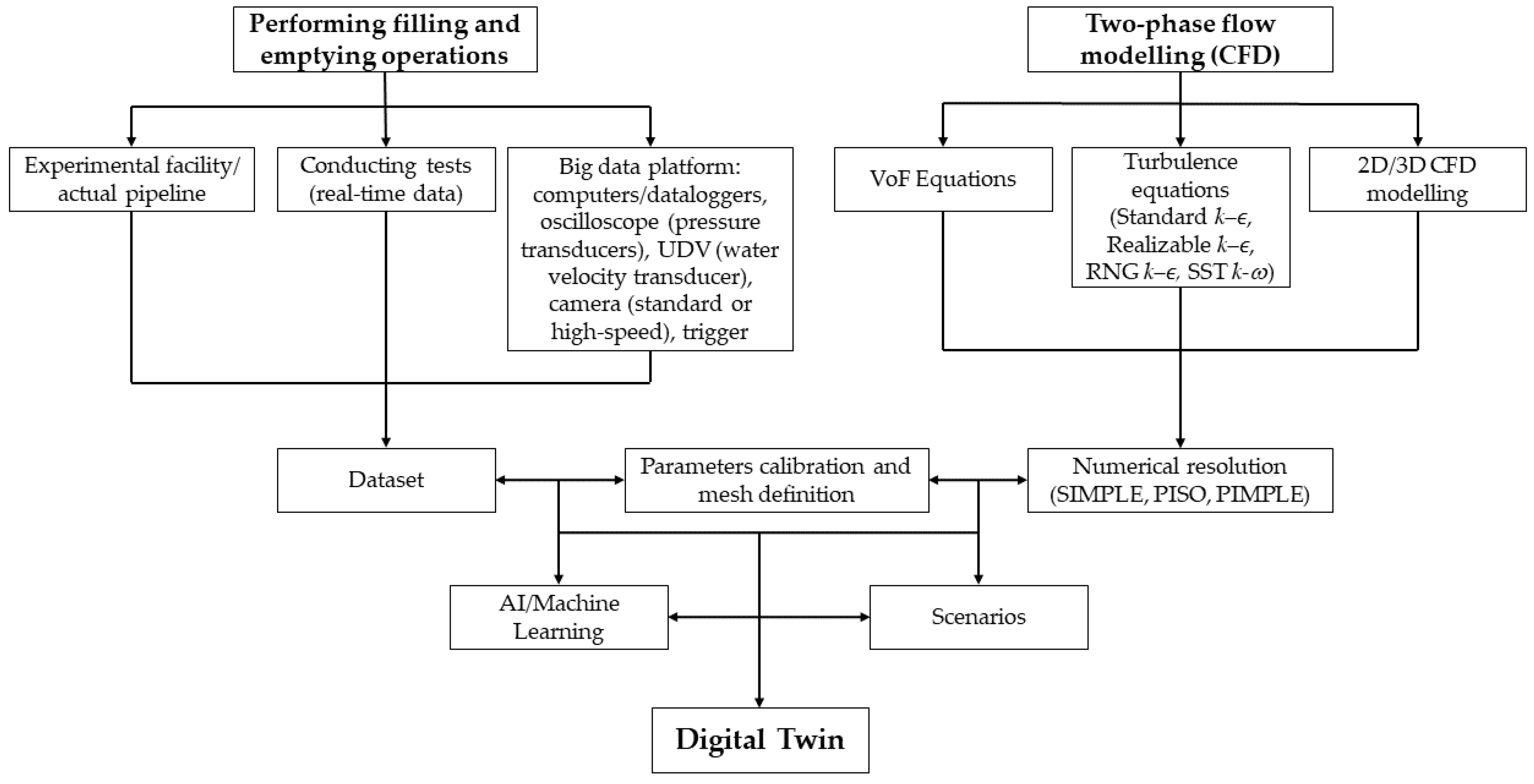
For developing Digital Twins to analyse the two-phase flow in pipes during filling and emptying procedures, real-time measured data are unified and, consequently, CFD simulations are performed. In this scenario, tests are performed in an experimental setup, recording data with the various equipment described in Section 2.2. For the CFD simulations, HVoF equations and turbulence models are defined. Experimental and simulation data are integrated into a dataset to calibrate the CFD model using mesh sensitivity analysis. By applying AI/machine learning tools, predictive analyses are performed that lead the user to identify the magnitude of the effects of air–water interaction in the study network through real-time records and, finally, represent these findings through a virtual model (DT) to test the most efficient conditions for decision-making on pressure conditions, trapped air volume, as well as the need for air valves in the study network. Figure 8 illustrates a DT framework which integrates CFD modelling to analyse hydraulic procedures.

In this section, an application of the DT based on CFD modelling is shown, taking two example cases as the filling and emptying procedures, as well as a summary of the correlational analysis of the pressure values between the real-time measurements and the DT with the dataset.

Scenarios of Table A1 were used for simulating filling procedures. On the other hand, information of Table A2 were used to simulate emptying procedures. Some modelling conditions are defined and shown in

Table 6. Modelling conditions for the application of Digital Twins through CFD modelling.

Scenario	Geometry	Mesh	Turbulence Model	Algorithm of Solution
Filling	3D	Unstructured	SST $k-\omega$	PISO
Empyting	2D	Structured	SST $k-\omega$	PISO

.

The CFD-based DTs were simulated using a two-way coupling approach with HVoF equations. This ensures a reciprocal interaction between water and air, allowing each phase to influence the other’s dynamics. Furthermore, the DTs were represented through the OpenFOAM v2412 software using a solver entitled compressibleInterFoam, which considers the compressibility of both air and water, with their respective compressibility differences (air is 20,000 times more compressible than water [70,71]). The effects of surface tension due to the application of the filling and emptying process in a small inner diameter pipe were considered (equal to 51.4 mm).

On the other hand, the modelling conditions for the filling and emptying procedures were based on the modelling conditions of Paternina-Verona et al. [59] for the filling procedures, as well as Hurtado-Misal et al. [29] and Paternina-Verona et al. [54] for the emptying procedures, highlighting some aspects such as mesh conditions with mesh independence analysis and physical boundary conditions. In this case, a turbulence model such as SST $k-\omega$ was applied for the filling procedures due to the good performance concerning adaptation in scenarios with high-pressure gradients. It was also used in emptying procedures since this turbulence model can represent the effects of the viscous layer as a function of the dynamic viscosity thus adequately simulating the fluid–pipe wall interaction independently in air and water.

5.1. Application of the Proposed Digital Twin for Filling Procedures

The Digital Twin application in this section discusses an analysis of the real-time measurements of the pressure patterns during filling procedures and describes the role of machine learning in determining possible efficient filling procedures. On the other hand, it also shows the development of the Digital Twin, describing the calibration methods and the validation of the numerical information with the measured data.

5.1.1. Data Analysis—Filling Procedures

The Digital Twin representing the filling procedures was refined from the hydraulic scenarios defined in Table A1. From these scenarios, pressure patterns were identified according to the presence or absence of air valves, air valve discharge diameter, and initial air pocket size. Figure 9 presents a sample of the real-time measurements carried out using the big data platform, which aids in analysing the pressure patterns according to the input data for filling procedures.

Figure 9 compares the pressure evolution in the different test scenarios. The results indicate that the most critical peak pressure occurs in the hydraulic filling conditions associated with the Type II scenario, specifically in Test No. 11, where a pressure peak exceeding 120 m-H₂O occurs within the first second. This behaviour suggests a rapid transition of flow conditions, likely influenced by the use of the D040 air valve, which does not effectively regulate the air expulsion rate, leading to sudden pressure surges. In contrast, the Type I scenario (Test No. 6), where no air valve is used, exhibits a more gradual pressure response, although with prolonged oscillations due to the trapped air and its compressibility effects.

In addition, differences in the pressure oscillation patterns are observed between the different scenarios. In the Type I and V scenarios, pressure oscillations are more pronounced and persist for extended periods, as the trapped air pocket is compressed without controlled expulsion. This situation is also evident in the Type III and VI scenario, where the S050 air valve is used but still allows considerable pressure oscillations, albeit slightly less extreme than in Types I and V.

The influence of initial air pocket size is also significant. A different pressure evolution is observed in Type V–VII, where the air pocket is increased by 1.5 m while maintaining the same conditions as Types I–IV. The increased air volume acts as a form of damping, altering the transient response. However, pressure fluctuations persist for extended periods without an air regulation mechanism. In contrast, when air valves are incorporated (Types VI and VII), pressure peaks are reduced, and the system stabilizes rapidly.

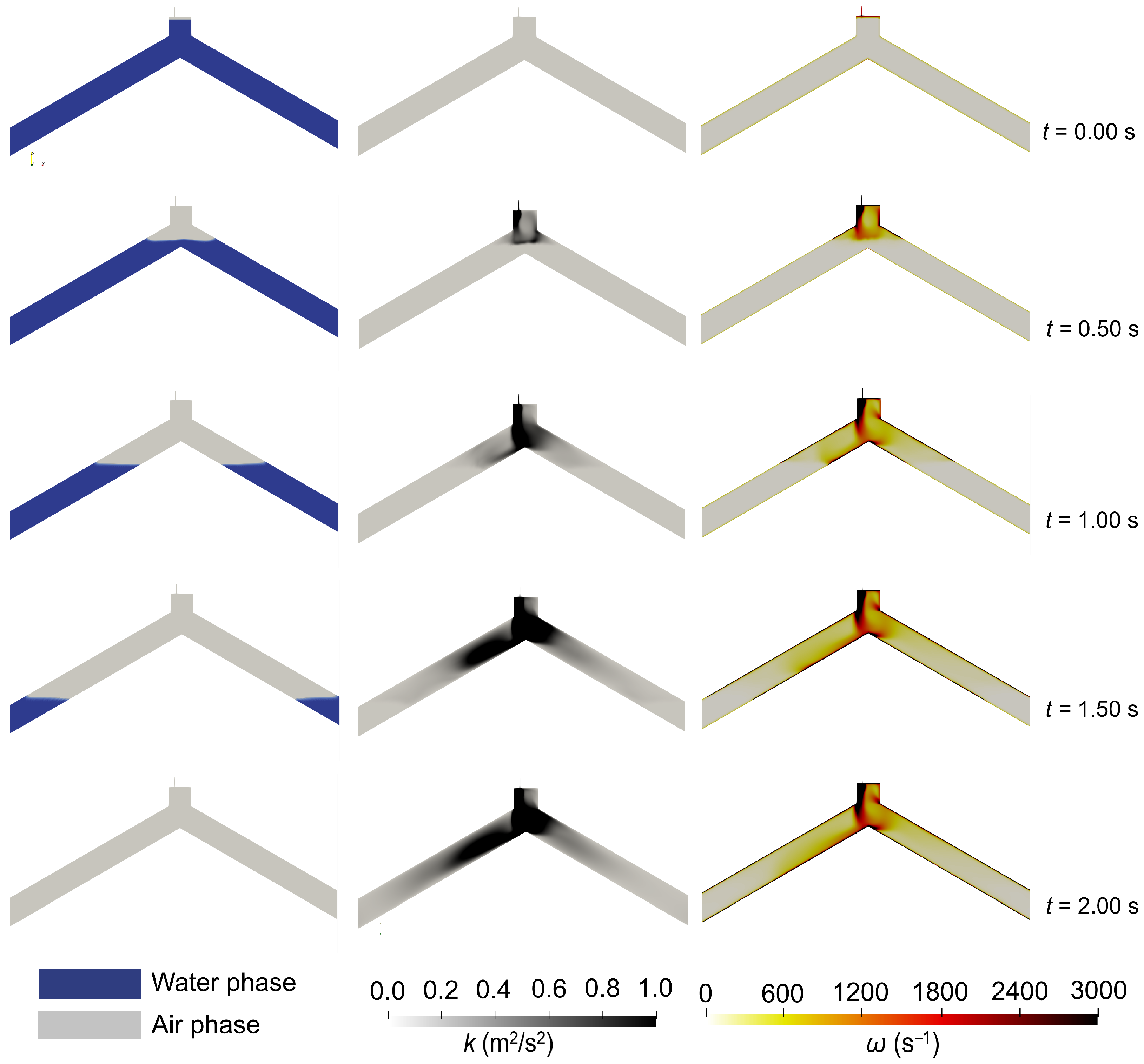
5.1.2. CFD-Based Digital Twin for Filling Procedures

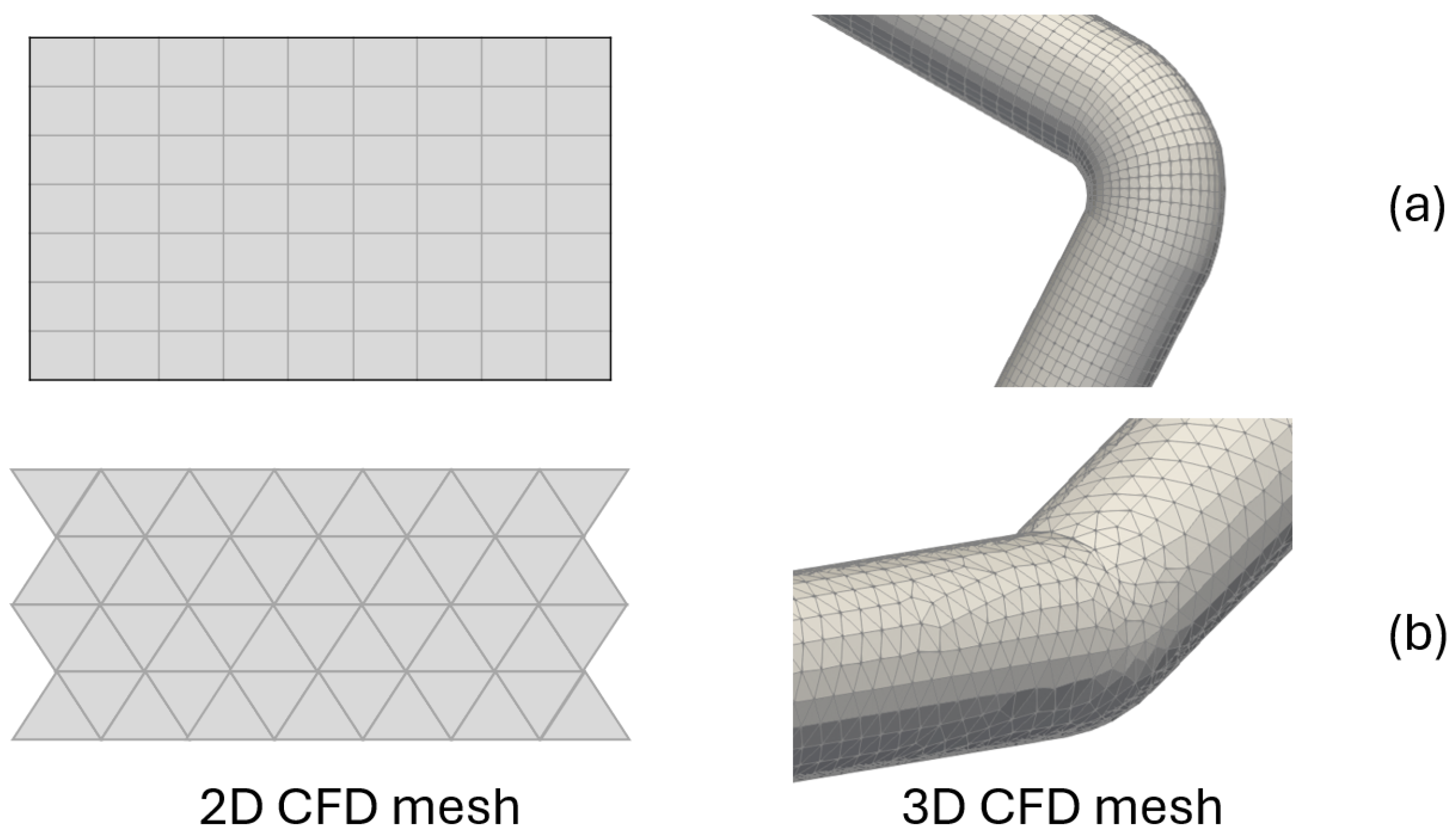
To develop a DT, a three-dimensional CFD model discretised by 330,793 tetrahedral elements was used. The number of elements was based on the mesh sensitivity of Paternina-Verona et al. [59]. The Digital Twin had three (3) boundaries and an inlet boundary, which was set using the absolute inlet pressure value (i.e., if the hydro-pneumatic tank pressure was 0.5 bar, the absolute pressure inlet value would be 151.325 Pa). The atmospheric pressure conditions determined the outlet boundary, and it was applied in scenarios where air valves were present. Additionally, the walls were another boundary governed by the no-slip function due to the friction generated by flow–pipeline interactions.

The CFD model was executed using the PISO algorithm with a variable Courant number, capped at a maximum of 0.9. This value, close to 1.0, was chosen to enhance the numerical analysis of air outflow through the air valve zone. The simulation time for filling procedures varied depending on the scenario. In the Type I and V scenarios (without air valves), the simulation required approximately two days to reproduce just two seconds of real-world behaviour, with an average time step of 4 × ${10}^{-5}$ s. In contrast, scenarios involving air valves (Type II, III, IV, VI, and VII) demanded significantly more computational effort, taking between 7 and 10 days with an average time step of 1 × ${10}^{-6}$ s. The reduced time step in these cases was necessary to capture airflow behaviour over the air valves accurately. All simulations were performed on an AMD Opteron processor (AMD, Santa Clara, CA, USA) with 16 cores, 32 threads, and 96 GB of RAM.

Figure 10 compares the real-time measurement of the trapped air pocket pressure and the three-dimensional CFD model, both associated with Test 38a (Table A1), and is shown as a representative example of a specific case study, illustrating in detail the evolution of trapped air pressure in a particular scenario. Test 38a highlights a good similarity between the measured information and the information calculated by the CFD model. At t = 0.00 s, the water phase, including the trapped air, rests. Subsequently, at t = 0.25 s, the water column rises to the pipe’s left branch. Consequently, the pressure in the air pocket gradually increases, reaching a pressure of 1.2 m-H₂O. At t = 0.50 s, the water column has reached the upper end of the hydraulic network, generating a backward movement of the water column through the upper zone of the pipe. At this instant, the trapped air pocket reaches the maximum overpressure value of 10.2 m-H₂O. At t = 1.5 s, the water column has displaced the volume of air trapped in the pipes outwards using a S050 air valve, and the water column has partially reached the upper zone of the pipe. At that instant, the trapped air pocket has started its second pressure pulse at t = 2.00 s.

To calibrate the DT to simulate the dataset, a compilation of the data measured concerning the air pocket pressure obtained in the DT is carried out, comparing the information of several tests associated with the different dataset typologies. Figure 11 compiles and synthesises the results of all the modelled scenarios, allowing for a global view of the DT performance under different conditions. This figure shows an adequate correlation between the measured values and those obtained in the DTs of the various scenarios associated with filling procedures.

To assess the correlation between the measured real-time data and the respective DT, the relative error equation is used for each dataset, and the results are then averaged. To calculate the relative error, Equation (12) is used.

$$\eta =\left|{\displaystyle \frac{x_{rt}-x_{dt}}{x_{rt}}}\right|$$

(12)

where $x_{rt}$ corresponds to the real-time measured value of the air pocket pressure, while $x_{dt}$ corresponds to the maximum pressure value of the DT. Based on the data in Figure 11, the correlational error between the datasets is 6.54%, indicating a satisfactory fit of the DT to the measured values in the filling scenarios analysed in this study. In particular, some correlated data are scattered concerning the fit line, especially in the range of values between 10 and 20 m-H₂O. These data in the mentioned range mostly correspond to the pressure measurements associated with secondary oscillations after the filling procedures, where the pipe acts as a buffer for the pipe material. This deviation is because the DT does not consider fluid–pipeline interactions.

5.2. Application of the Proposed Digital Twin for Emptying Procedures

The Digital Twin application in this section focuses on analysing the real-time pressure measurements during emptying procedures and exploring the role of machine learning in identifying efficient drainage strategies. Additionally, it examines the system’s behaviour by comparing numerical predictions with measured data.

5.2.1. Data Analysis—Emptying Procedures

In the case of the Digital Twin for the representation of emptying procedures, some sensitivity parameters such as the initial size of the trapped air pocket, the opening percentage of the drain valves, as well as the air intake orifice diameter of the air valves are taken into account. Figure 12 offers a sample of the identified behaviours, showing that the most critical vacuum pressures are associated with the Type II scenarios (with a value of 9.32 m-H₂O in Test 3, where there are no air valves, and the valve opening is complete). A different behaviour occurs in the Type I scenario, where the opening of the drain valves is partial, generating a controlled drainage process and a damping of the vacuum pressures and thus resulting in a value of 9.73 m-H₂O in Test 1. In the case of the Type III scenario, the lengths of the air pockets are longer compared to those presented in the Type II scenario, and the conditions of whole drain valve opening are maintained, thereby offering a minimum pressure of 9.51 m-H₂O in Test 5.

Also, the differences in pressure patterns between the emptying procedures with and without air valves are shown. Figure 12 shows that in the emptying scenarios without air valves (Type I, II and III), pressure oscillations occur, which are dissipated because of energy damping by the trapped air and the pipe material, whereas in the scenarios with air valves (Type IV and V), the minimum vacuum pressures are less than the scenarios without air valves.

In the Type IV scenario, an air valve with a diameter of 3.175 mm is used, and in a study test (Test 7), a minimum vacuum pressure of 9.56 m-H₂O is shown. In contrast, in the V scenario, an air valve with an orifice inlet diameter of 9.375 mm is applied thus generating a minimum pressure of 10.14 m-H₂O. Consequently, a rapid filling procedure takes place, since, in the other scenarios (Type I–IV), the pressure takes more than 8 s to recover the atmospheric conditions, which suggests that the emptying process for that point in time has not finished; whereas, in the Type V scenario (Test 12), the atmospheric pressure recovers its atmospheric conditions at 6.5 s, which is related to the total emptying of the water from the pipe at that point in time.

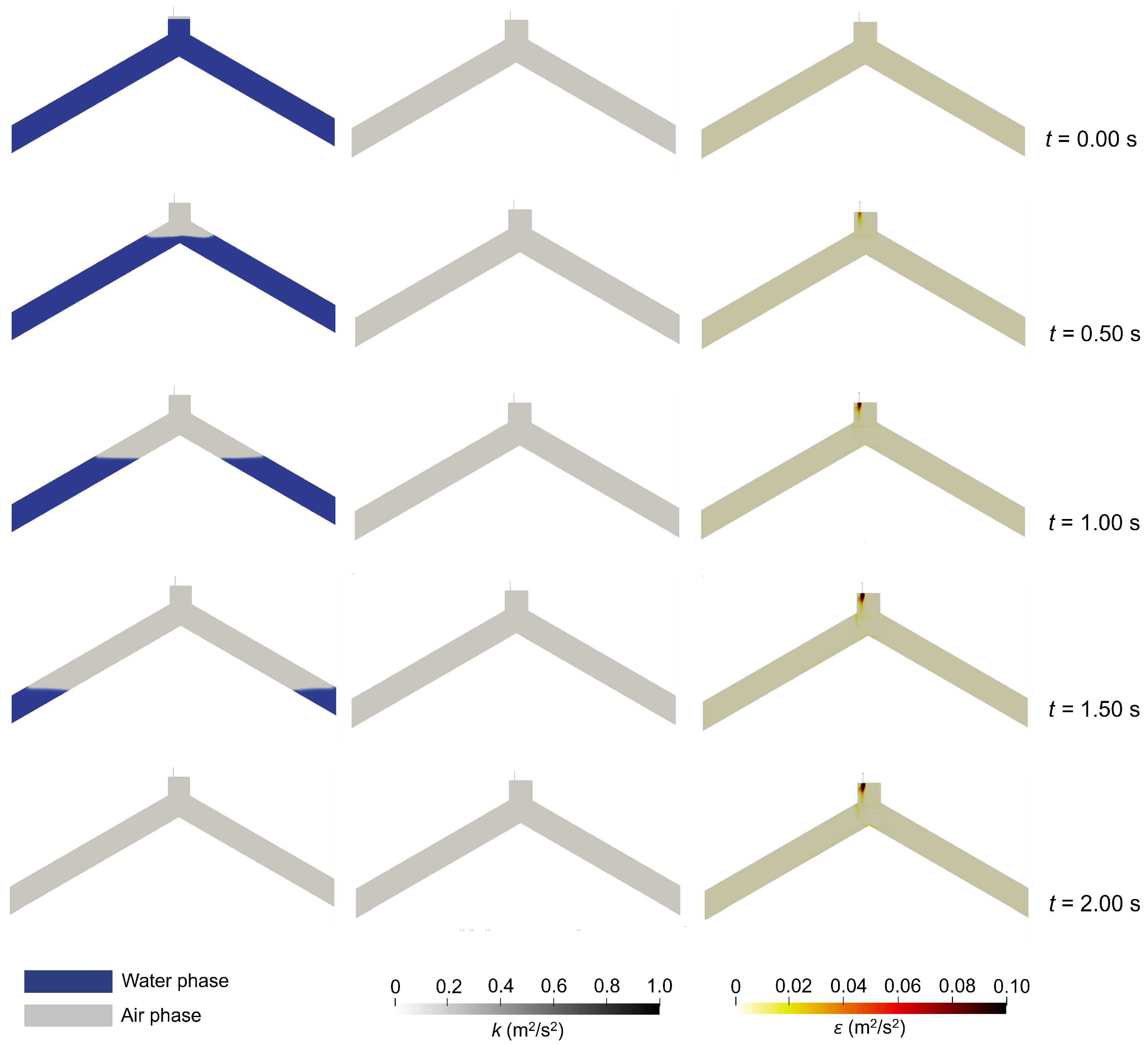
5.2.2. CFD-Based Digital Twin for Emptying Procedures

In this case, a DT is used based on a two-dimensional CFD simulation discretised by 26,130 hexahedral cells. The number of elements is based on the mesh sensitivity of Paternina-Verona et al. [54] and Hurtado-Misal et al. [29]. The Digital Twin for emptying procedures has four (4) boundary conditions. The inlet boundary allows for air admission and is governed by an atmospheric pressure condition, which is only applied in the Type IV and V scenarios where air valves are present. The outlet boundary is also determined by atmospheric pressure and corresponds to the water discharge during emptying. The walls are subject to no-slip conditions, ensuring realistic fluid behaviour along solid surfaces. A Valve Sliding Interface (VSI) function is implemented, acting as a dynamic mesh that simulates a shut-off valve, allowing for controlled drainage.

Using a PISO algorithm, the DTs were run using a maximum Courant number of 0.7 to guarantee numerical stability during the simulation. The average time step was 1 × ${10}^{-4}$ s, and the model took approximately 4 days to represent the equivalent of 8 s of the real-world behaviour.

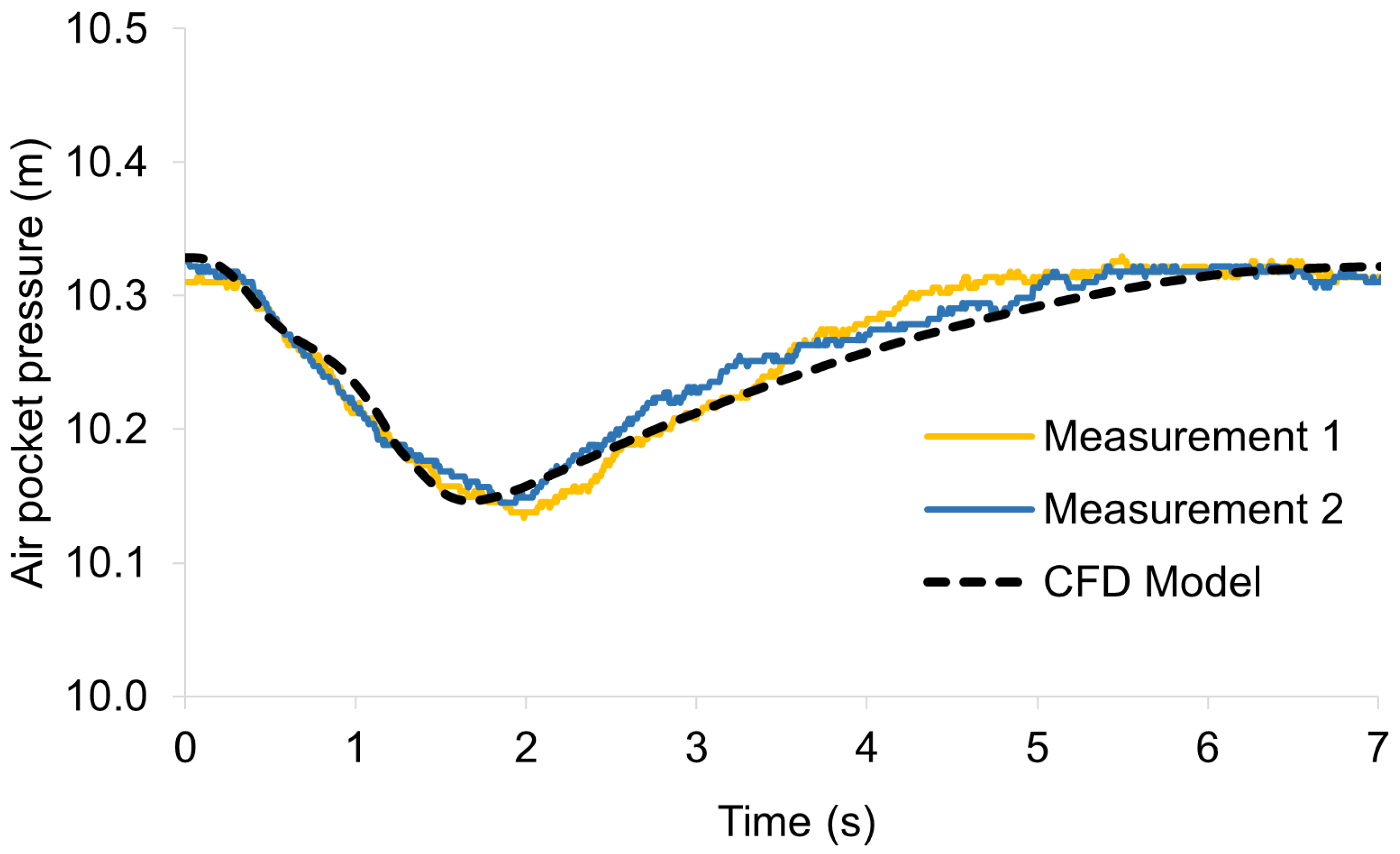
Figure 13 shows a comparison between the real-time measurements by a pressure transducer and the numerical patterns of air pocket pressure during the emptying process of Test 12 (Table A2—Type V), in which a similarity is identified between the patterns measured in real time and those obtained in the two-dimensional CFD model. In this case, the pressure drops gradually from the initial instant to t = 2.0 s due to the gradual opening of the drain valves for a duration of 1.6 s. During this first time point, the air volume expands. Subsequently, the pressure increases in a controlled manner due to the admission of air through the air valve D040 thus generating a controlled emptying in a time of 7 s.

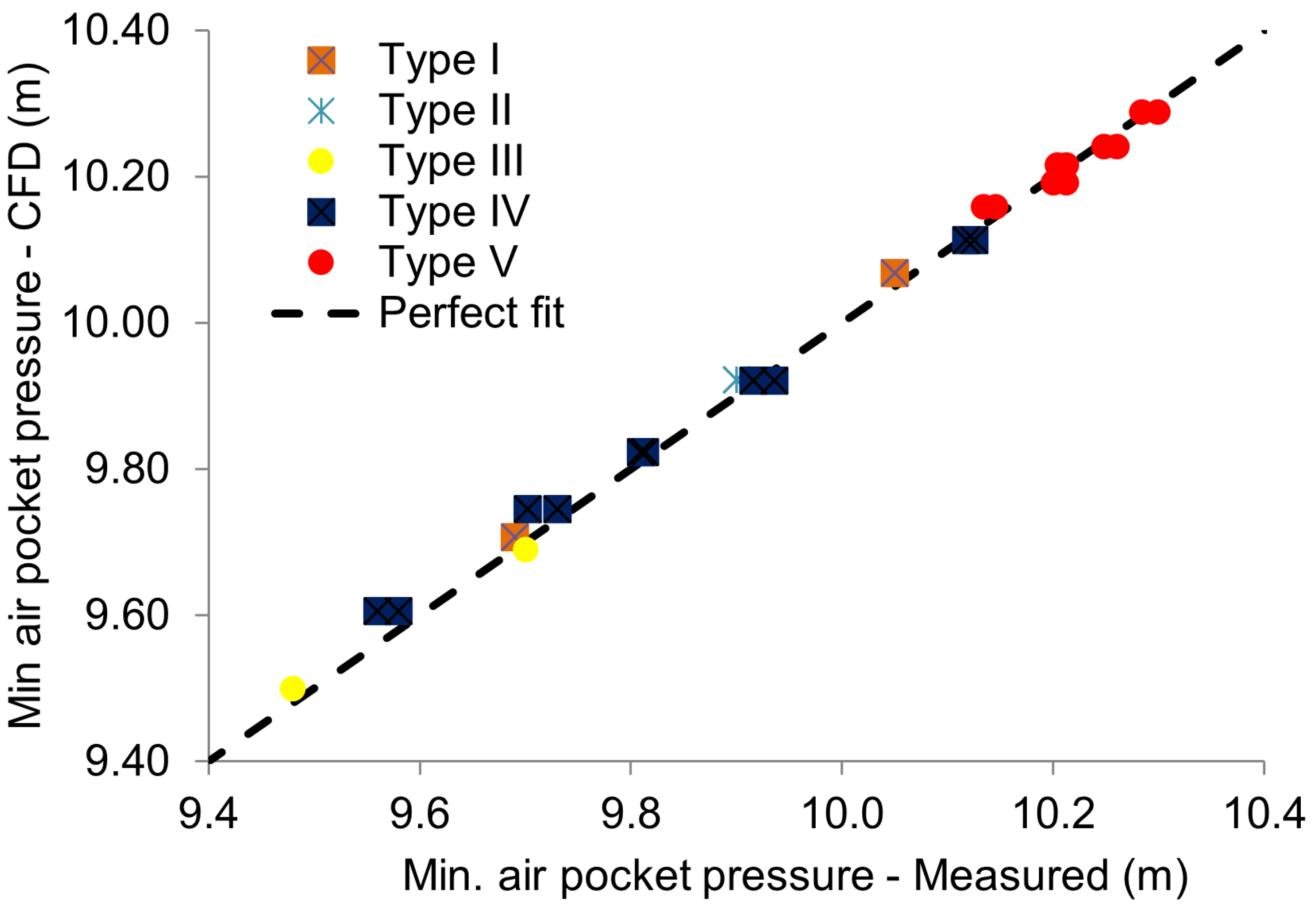
As in the representation of Test 12 (see Figure 13), the DTs proposed for the emptying procedures were applied to corroborate the reliability of its development in the different types of emptying scenarios set out in Table A2. In this case, a comparison was made between the minimum peak values of the measured air pocket pressure and those obtained in the CFD model that integrated the DT, as shown in Figure 14, where an adequate fit, with a relative error of 0.16%, was observed between both values along the perfect fit line. This validates its applicability for simulating hydraulic scenarios involving trapped air, enabling the prediction of critical events associated with air management in pipe networks.

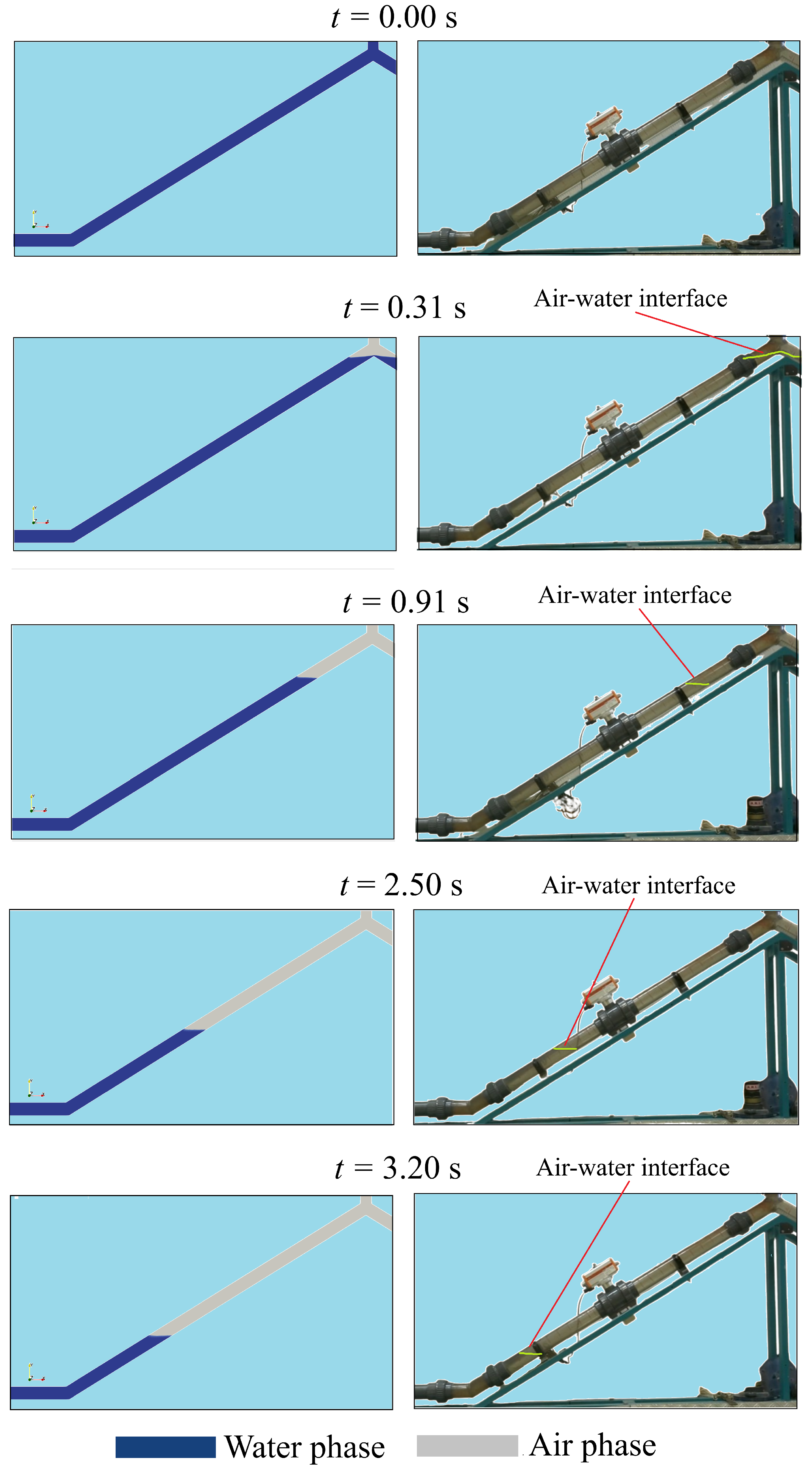
When pipelines are transparent, video data allow for the identification of air–water interaction phenomena that help to validate the proper development of the CFD model and verify the physical behaviour of both fluids. Figure 15 compares the motion of the air–water interface detected by camera frames, as well as the contours of the air–water phases of the CFD model that were captured using the proposed DT.

5.3. Application of Machine Learning Model

Filling and emptying processes are essential operations that water utilities must perform using the CFD modelling. In the existing pipelines, these simulations can take approximately 2.5 months [72]. Given the urgency of interventions, water utilities cannot afford such lengthy simulation times.

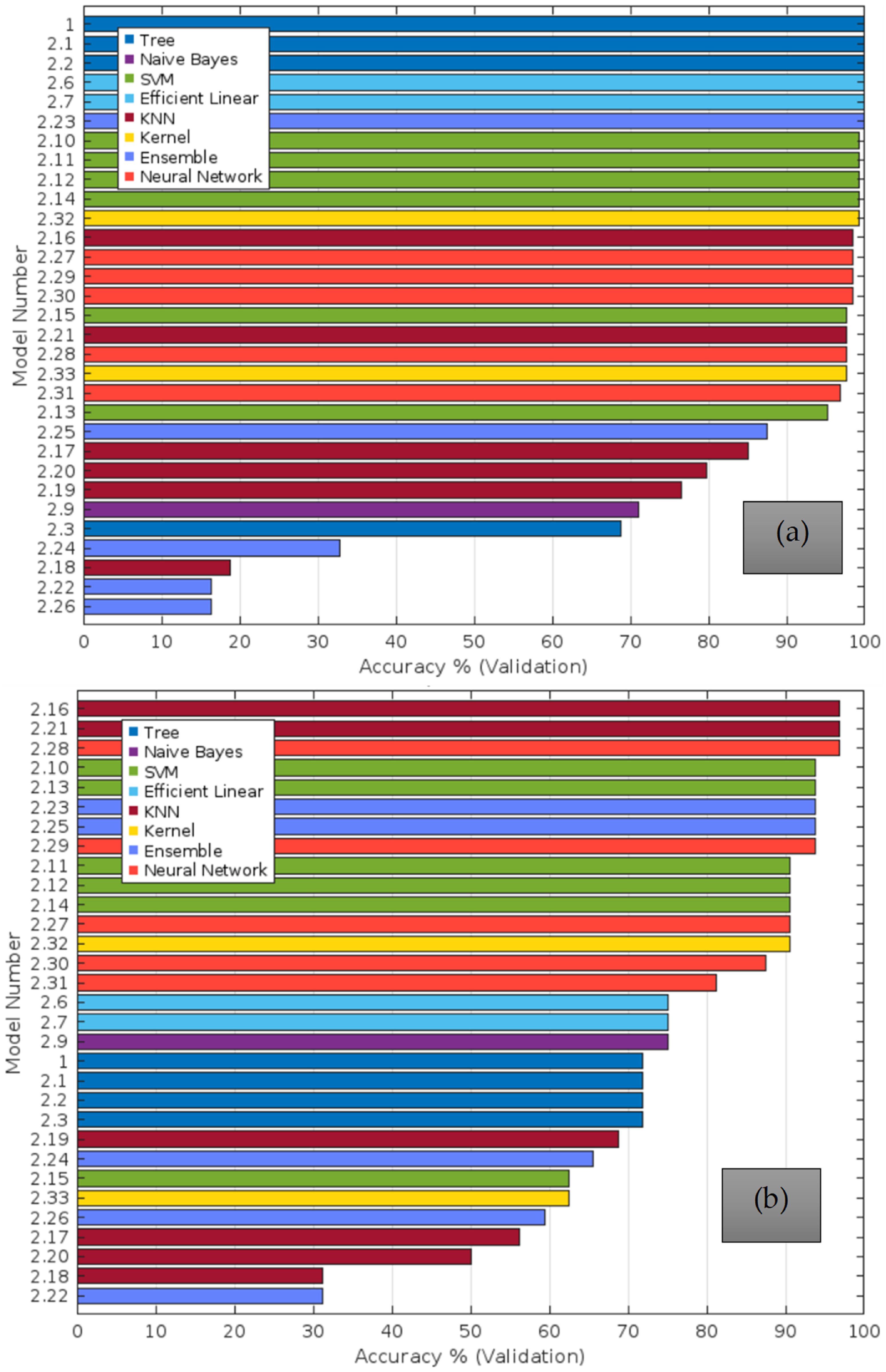
To address this challenge, the datasets presented in Table A1 and Table A2 were used to train a predictive model capable of forecasting the behaviour of filling and emptying procedures. The MATLAB vR2020a software validated a reliable machine learning model, testing 31 algorithms. The numerical accuracy rates of various classification learner algorithms—including decision trees, support vector machines, nearest neighbour classifiers, and ensemble classifiers—are illustrated in Figure 16. Among these, for filling processes, the tree, efficient linear, and ensemble models proved the most suitable for accurately replicating the complex air–water interactions with an accuracy of 100%; while for the emptying procedures, the KNN models provided the best responses with a fit of 96.9%.

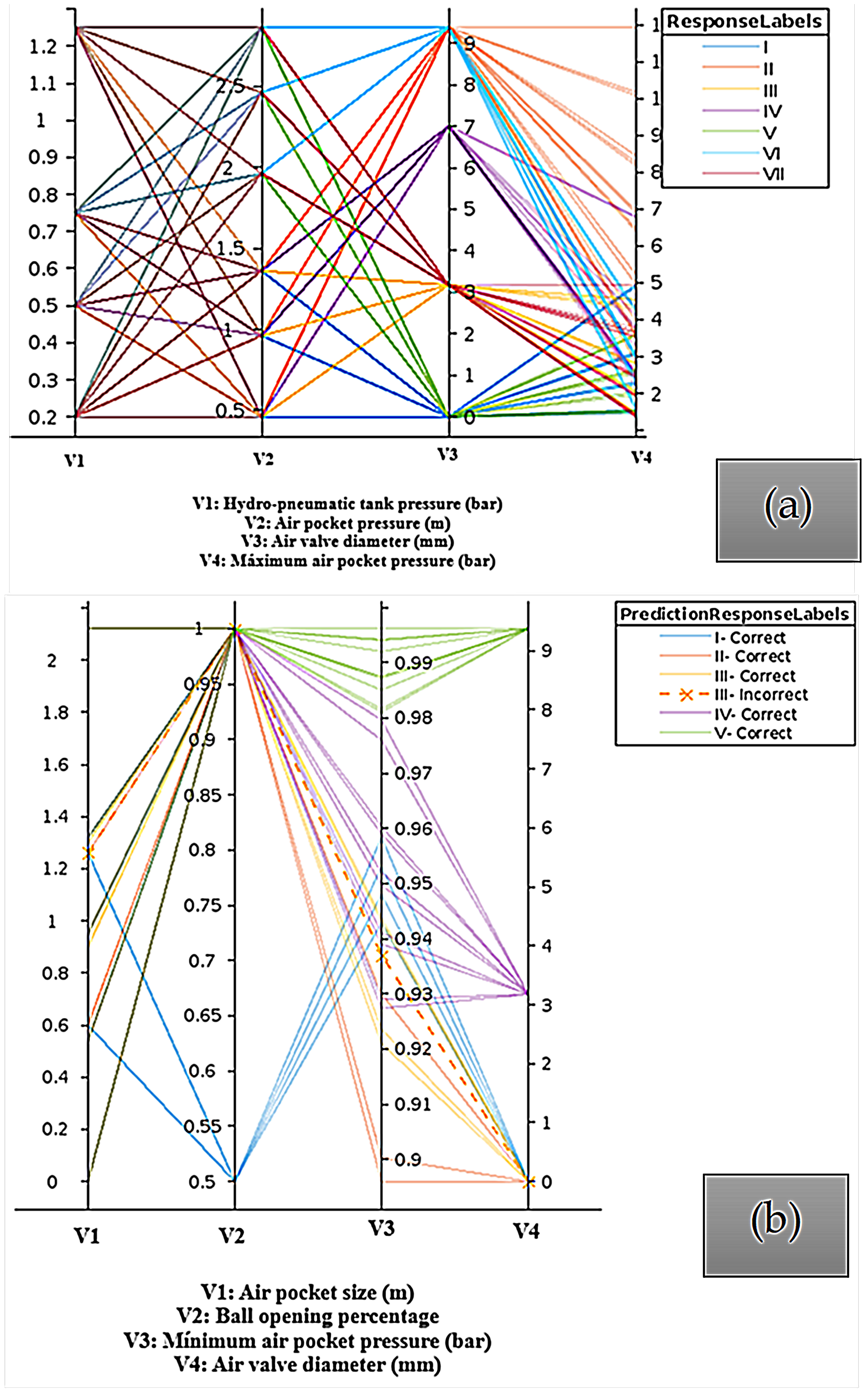
The following variables were used to classify the scenarios for implementing these algorithms (see Appendix A): initial hydro-pneumatic pressure in the tank ($p_0$); initial air pocket size ($x_0$); internal pipe diameter (51.4 mm); maximum/minimum pressure during the transient event; and air valve diameter. Figure 17 illustrates the parallel coordinates for the predictions. Only one incorrect prediction was reached for the emptying processes.

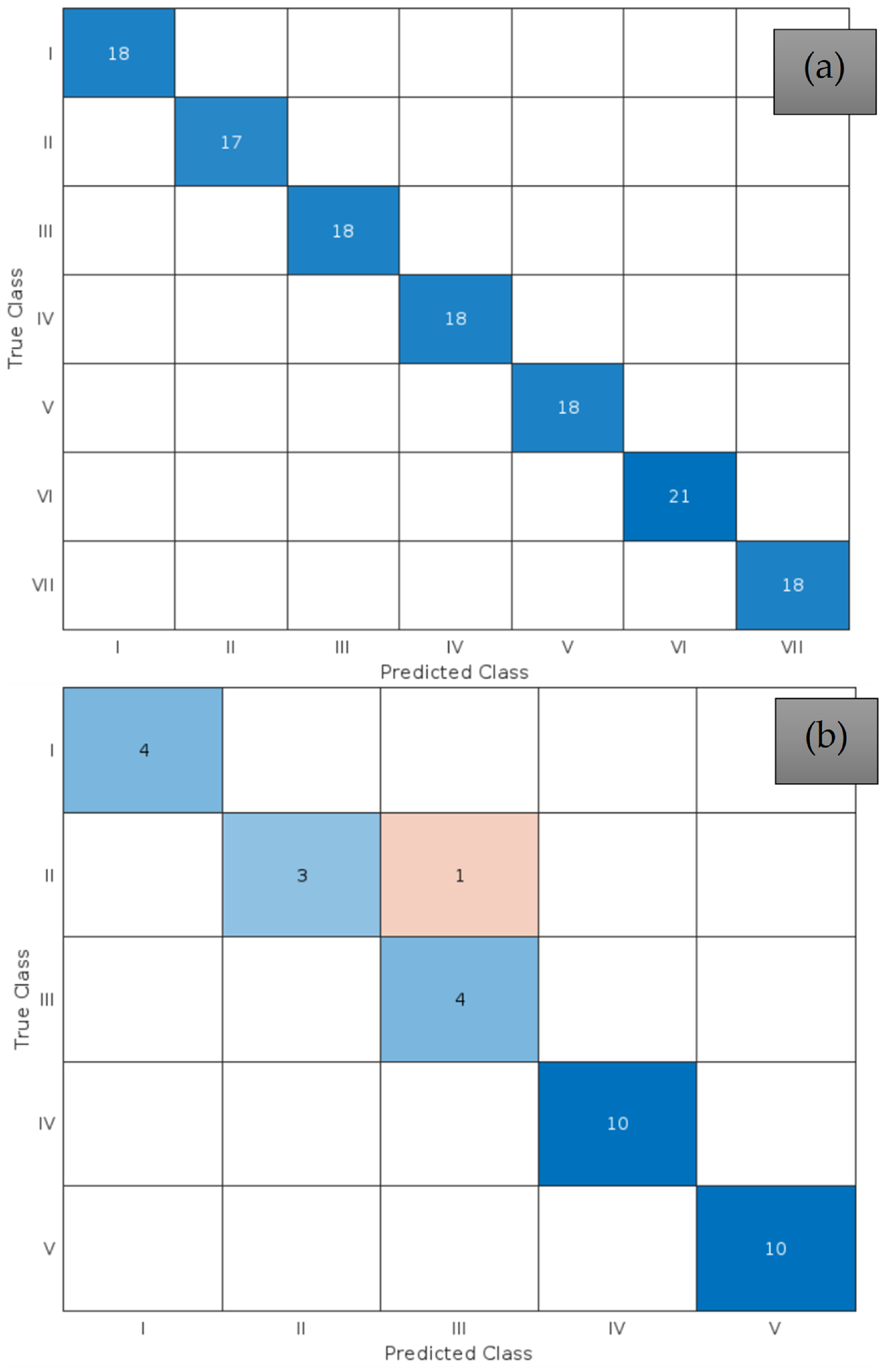
Figure 18 presents the confusion matrix for the best solution for the filling and emptying operations, allowing for an assessment of validation accuracy.

The trained models effectively captured the hazardous pressure peaks generated in the Type II scenario for the filling processes (see Figure 9). In this scenario, a pressure head peak of 123 m was observed, approaching the nominal pipe pressure of 163.2 m (PN 16). This occurs when an air valve with a high expelled air capacity induces dangerous pressure surges. It is not a common situation but depending on initial conditions, it can occur. This finding is particularly significant, as it highlights the ability of machine learning techniques to identify undesirable conditions, thereby helping to prevent pipe failure in existing water pipelines. Similarly, for emptying processes, the adopted machine learning model can follow the tendency of air–water interactions with and without air valves, providing a practical tool for detecting collapse conditions depending on soil conditions and stiffness pipe class.

6. Discussion

The CFD-Based Digital Twins have proven to be a robust approach to analysing transient two-phase flows in pipeline filling and emptying operations. This study has demonstrated the capacity of DTs to replicate complex hydraulic phenomena, offering a predictive tool for optimising operational procedures.

One of the key findings of this research is the role of air pockets in influencing transient pressure conditions. The results show that entrapped air pockets significantly affect both the filling and emptying processes, with their size and distribution altering the pressure response. In filling procedures, large air pockets cause rapid pressure surges due to compression effects, particularly when air expulsion is not adequately controlled (e.g., Type II with an AV D040 and III with an AV S050). Conversely, air pockets contribute to vacuum pressure formation in emptying processes, which can lead to structural risks in the pipeline system if not properly managed. The results highlight the impact of different air valve configurations on the pressure regulation for emptying procedures. Scenarios incorporating air valves, such as Type IV and V for the emptying procedures, exhibit smoother pressure transitions and reduced pressure peaks compared to the cases without air regulation. This is consistent with the previous research indicating that controlled air admission and expulsion mechanisms are fundamental to mitigate hydraulic transients Carlos et al. [73]. In the case of the study of air valves in filling procedures, it is observed that the use of a 7 mm orifice (Type IV) demonstrates a more gradual pressure variation, suggesting that optimising valve size and placement can enhance system stability.

The comparison between real-time pressure measurements and numerical data confirmed the reliability of the DT models. Calibration efforts, including mesh sensitivity analysis and turbulence model selection, accurately represented transient hydraulic behaviours. The DTs demonstrated an adequate predictive capability, obtaining the time series associated with the evolution of hydraulic–thermodynamic parameters at any point in the geometric domain, such as pressure and velocity, as well as the opportunity to visualise the spatial distribution of these same variables at different points in time. The differences between the numerical and measured values are slight, with relative errors remaining within the acceptable limits, typically below 6.54% for the filling procedures and 0.16% for the emptying procedures. However, some discrepancies were noted in the secondary oscillations post-filling (in the case of the filling procedures), likely due to pipe–wall interactions that were not explicitly accounted for in the model.

A 2D approach is chosen to simulate emptying procedures and efficiently capture the evolution of air pockets and vacuum pressures along the pipeline. Since the flow is predominantly stratified (as shown in Figure 15 in Test 12 as an example), with air entering the system from the highest point and water draining from the lowest, a two-dimensional model provides sufficient resolution while optimising computational resources.

For filling procedures, a 3D CFD model is necessary to capture the complex dynamics of air compression and expulsion. Unlike the emptying processes, filling involves a more intricate interaction between air and water, with significant pressure surges and turbulent mixing occurring in multiple directions. The three-dimensional approach allows for a more detailed representation of the air pockets’ spatial evolution, the effects of valve positioning, and the potential for asymmetric flow patterns that cannot be captured in a 2D framework.

On the other hand, the potential of integrating machine learning techniques within the Digital Twin framework is highlighted. By training predictive models using datasets from real-time monitoring and CFD simulations, the DT can identify unfavourable conditions, such as excessive vacuum or high surge pressures. This capability can assist in decision-making by recommending optimal valve operation strategies and predicting potential failure risks before they occur. However, some limitations must be considered. ML models may struggle with highly complex or unforeseen hydraulic scenarios that are not well represented in the training phase. Furthermore, the computational cost of real-time learning and inference can be significant, especially for large-scale pipeline systems with continuously changing conditions. Despite these limitations, the integration of machine learning into the Digital Twin framework represents a valuable advance in optimising pipeline operations and safety thus leveraging predictive capabilities through real-time data and CFD modelling.

7. Conclusions

This research presents a Digital Twin framework based on CFD modelling for analysing and optimising the filling and emptying procedures in pressurized pipelines. The main conclusions drawn from this study are as follows:

• Entrapped air pockets play a critical role in transient pressure fluctuations during filling and emptying operations. Their size and distribution significantly impact the hydraulic response, with large air pockets contributing to extreme pressure variations.
• The implementation of air valves and orifices effectively mitigates pressure surges and vacuum formation. The results indicate that controlled air expulsion reduces overpressures during filling, while air admission mechanisms minimize vacuum conditions during emptying.
• The Digital Twin models accurately replicate pressure dynamics, demonstrating a good agreement between the real-time measurements and the numerical simulations.
• Machine learning techniques enhance decision-making by identifying critical hydraulic scenarios and optimising pressure management in pipeline filling and emptying processes. They enable the prediction of optimal pressure heads for filling and the most effective valve operation settings for emptying, while also assessing the influence of air valves in both cases. This demonstrates the reliability of ML models in forecasting pipeline behaviour, not only under standard conditions (Scenarios I, III–VII) but also in situations where large air valves may induce higher overpressures than smaller ones (Scenario II), as observed by Aguirre-Mendoza et al. [56]. Additionally, for the emptying procedures, ML models can help detect critical sub-atmospheric pressure levels that must be monitored to prevent pipeline collapse. Using ML techniques, it is possible to enhance computational efficiency and reduce the time required by CFD models when predicting these processes in real pipelines.

Integrating a CFD-based Digital Twin with a machine learning model allows users to identify key hydraulic phenomena, such as maximum and minimum pressures, by leveraging both dataset information and CFD-simulated models. This approach enables a more comprehensive analysis of pipeline behaviour. In addition, the CFD-based Digital Twin can be used to test scenarios beyond those included in the dataset, identify some hydraulic phenomena conditions without requiring further CFD simulations, providing a valuable tool for operational decision-making to ensure safe and optimal filling and emptying conditions in a short time.

It is important to highlight that improper manoeuvres can compromise the integrity of these systems under extreme pressure. Inadequate operations may lead to an increased incidence of pipeline ruptures, resulting in high costs for maintenance and repair programmes and elevated leakage volumes in water installations, which present a challenge for both developing and developed countries. Generating scenarios using the proposed Digital Twin can be a powerful tool for preventing pipeline ruptures and stopping new leakages.

Unlike the proposed Digital Twin, the current recommendations and manuals, such as AWWA M51, do not provide sufficient tools for adequate modelling. This research exemplifies the implementation of a Digital Twin applied to an experimental facility located in the Hydraulics Laboratory of the Instituto Superior Técnico (IST) at the University of Lisbon. Additionally, a comprehensive dataset of filling and emptying scenarios is presented in the Supplementary Materials, which water utilities can utilise to reproduce these results.

For future work, the application of a Digital Twin scheme for large-scale hydraulic pipelines is relevant, basing machine learning on the safety conditions of the hydraulic system (resistance of pipe materials) and on the national/international regulations for the control of filling/emptying procedures (min/max velocities and pressures). In addition, the numerical modelling should focus on refining fluid–structure interaction models to account for the secondary oscillations due to pipe–wall interactions and expand the DT framework to real-world water distribution networks.

References

1. Ayadi, A.; Ghorbel, O.; BenSalah, M.; Abid, M. A framework of monitoring water pipeline techniques based on sensors technologies. J. King Saud Univ. Comput. Inf. Sci. 2022, 34, 47–57. [Google Scholar] [CrossRef]
2. Martin, A.; Delgado-Aguiñaga, J.; Puig, V. Control of transients in drinking water networks. Control Eng. Pract. 2022, 119, 104986. [Google Scholar] [CrossRef]
3. Zhou, L.; Liu, D.; Karney, B. Investigation of hydraulic transients of two entrapped air pockets in a water pipeline. J. Hydraul. Eng. 2013, 139, 949–959. [Google Scholar] [CrossRef]
4. Zhou, L.; Wang, H.; Karney, B.; Liu, D.; Wang, P.; Guo, S. Dynamic behavior of entrapped air pocket in a water filling pipeline. J. Hydraul. Eng. 2018, 144, 04018045. [Google Scholar] [CrossRef]
5. Besharat, M.; Coronado-Hernández, O.E.; Fuertes-Miquel, V.S.; Viseu, M.T.; Ramos, H.M. Computational fluid dynamics for sub-atmospheric pressure analysis in pipe drainage. J. Hydraul. Res. 2019, 58, 553–565. [Google Scholar] [CrossRef]
6. Paternina-Verona, D.A.; Coronado-Hernández, O.E.; Aguirre-Mendoza, A.M.; Espinoza-Román, H.G.; Fuertes-Miquel, V.S. Three-dimensional simulation of transient flows during the emptying of pipes with entrapped air. J. Hydraul. Eng. 2023, 149, 04023007. [Google Scholar] [CrossRef]
7. Mitkov, R.; Pantusheva, M.; Petrova-Antonova, D.; Naserentin, V.; Logg, A. The Role of Computational Fluid Dynamics within City Digital Twins: Opportunities and Challenges. ISPRS Ann. Photogramm. Remote Sens. Spat. Inf. Sci. 2024, 10, 131–136. [Google Scholar] [CrossRef]
8. Therrien, J.D.; Nicolaï, N.; Vanrolleghem, P.A. A critical review of the data pipeline: How wastewater system operation flows from data to intelligence. Water Sci. Technol. 2020, 82, 2613–2634. [Google Scholar] [CrossRef]
9. Hu, W.; Lim, K.Y.H.; Cai, Y. Digital twin and industry 4.0 enablers in building and construction: A survey. Buildings 2022, 12, 2004. [Google Scholar] [CrossRef]
10. Shafiee, M.E.; Barker, Z.; Rasekh, A. Enhancing water system models by integrating big data. Sustain. Cities Soc. 2018, 37, 485–491. [Google Scholar] [CrossRef]
11. Berglund, E.Z.; Shafiee, M.E.; Xing, L.; Wen, J. Digital twins for water distribution systems. J. Water Resour. Plan. Manag. 2023, 149, 02523001. [Google Scholar] [CrossRef]
12. Curl, J.M.; Nading, T.; Hegger, K.; Barhoumi, A.; Smoczynski, M. Digital twins: The next generation of water treatment technology. J. Am. Water Works Assoc. 2019, 111, 52–58. [Google Scholar] [CrossRef]
13. Wu, Z.Y.; Chew, A.; Meng, X.; Cai, J.; Pok, J.; Kalfarisi, R.; Lai, K.C.; Hew, S.F.; Wong, J.J. High fidelity digital twin-based anomaly detection and localization for smart water grid operation management. Sustain. Cities Soc. 2023, 91, 104446. [Google Scholar] [CrossRef]
14. Pesantez, J.E.; Alghamdi, F.; Sabu, S.; Mahinthakumar, G.; Berglund, E.Z. Using a digital twin to explore water infrastructure impacts during the COVID-19 pandemic. Sustain. Cities Soc. 2022, 77, 103520. [Google Scholar] [CrossRef]
15. Fabbiano, L.; Vacca, G.; Dinardo, G. Smart water grid: A smart methodology to detect leaks in water distribution networks. Measurement 2020, 151, 107260. [Google Scholar] [CrossRef]
16. Romero, L.; Pérez-Sánchez, M.; López Jiménez, P.A. Improvement of sustainability indicators when traditional water management changes: A case study in Alicante (Spain). AIMS Environ. Sci. 2017, 4, 502–522. [Google Scholar] [CrossRef]
17. Ntuli, N.; Abu-Mahfouz, A. A simple security architecture for smart water management system. Procedia Comput. Sci. 2016, 83, 1164–1169. [Google Scholar] [CrossRef]
18. Boyle, T.; Giurco, D.; Mukheibir, P.; Liu, A.; Moy, C.; White, S.; Stewart, R. Intelligent metering for urban water: A review. Water 2013, 5, 1052–1081. [Google Scholar] [CrossRef]
19. Ramos, H.M.; Kuriqi, A.; Coronado-Hernández, O.E.; López-Jiménez, P.A.; Pérez-Sánchez, M. Are digital twins improving urban-water systems efficiency and sustainable development goals? Urban Water J. 2023, 21, 1164–1175. [Google Scholar] [CrossRef]
20. Conejos Fuertes, P.; Martínez Alzamora, F.; Hervás Carot, M.; Alonso Campos, J. Building and exploiting a Digital Twin for the management of drinking water distribution networks. Urban Water J. 2020, 17, 704–713. [Google Scholar] [CrossRef]
21. Lui, X.; Zhang, L. CFD Applications in Water, Wastewater, and Stormwater; ASCE: Reston, VA, USA, 2019. [Google Scholar]
22. American Society of Mechanical Engineers. Standard for Verification and Validation in Computational Fluid Dynamics and Heat Transfer: An American National Standard; American Society of Mechanical Engineers: New York City, NY, USA, 2009. [Google Scholar]
23. Cataño-Lopera, Y.A.; Spelman, D.; Yee, T.; Pathapati, S.; Beck, K.J.; Lee, J.; Knatz, C.; Wang, R.Q.; Zhang, J.; Camacho-Rincon, R.; et al. Best Practices for Computational Fluid Dynamic Applications in Water Infrastructure. J. Environ. Eng. 2023, 149, 03123003. [Google Scholar] [CrossRef]
24. Besharat, M.; Coronado-Hernández, O.E.; Fuertes-Miquel, V.S.; Viseu, M.T.; Ramos, H.M. Backflow air and pressure analysis in emptying a pipeline containing an entrapped air pocket. Urban Water J. 2018, 15, 769–779. [Google Scholar] [CrossRef]
25. Anderson, D.; Tannehill, J.C.; Pletcher, R.H.; Munipalli, R.; Shankar, V. Computational Fluid Mechanics and Heat Transfer; CRC Press: Boca Raton, FL, USA, 2020. [Google Scholar]
26. Liu, D.; Zhou, L. Numerical simulation of transient flow in pressurized water pipeline with trapped air mass. In Proceedings of the 2009 Asia-Pacific Power and Energy Engineering Conference, Wuhan, China, 27–31 March 2009; pp. 1–4. [Google Scholar]
27. Zhou, L.; Liu, D.Y.; Ou, C.Q. Simulation of flow transients in a water filling pipe containing entrapped air pocket with VOF model. Eng. Appl. Comput. Fluid Mech. 2011, 5, 127–140. [Google Scholar] [CrossRef]
28. Besharat, M.; Tarinejad, R.; Aalami, M.T.; Ramos, H.M. Study of a compressed air vessel for controlling the pressure surge in water networks: CFD and experimental analysis. Water Resour. Manag. 2016, 30, 2687–2702. [Google Scholar] [CrossRef]
29. Hurtado-Misal, A.D.; Hernández-Sanjuan, D.; Coronado-Hernández, O.E.; Espinoza-Román, H.; Fuertes-Miquel, V.S. Analysis of Sub-Atmospheric Pressures during Emptying of an Irregular Pipeline without an Air Valve Using a 2D CFD Model. Water 2021, 13, 2526. [Google Scholar] [CrossRef]
30. Martins, N.M.; Delgado, J.N.; Ramos, H.M.; Covas, D.I. Maximum transient pressures in a rapidly filling pipeline with entrapped air using a CFD model. J. Hydraul. Res. 2017, 55, 506–519. [Google Scholar] [CrossRef]
31. Martins, S. Pressurization Dynamics of Hydraulic Systems with Entrapped Air. Ph.D. Dissertation, Instituto Superior Técnico, Universidade de Lisboa, Lisboa, Portugal, 2012. (In Portuguese). [Google Scholar]
32. Li, L.; Zhu, D.Z.; Huang, B. Analysis of pressure transient following rapid filling of a vented horizontal pipe. Water 2018, 10, 1698. [Google Scholar] [CrossRef]
33. Chan, S.N.; Cong, J.; Lee, J.H. 3D numerical modeling of geyser formation by release of entrapped air from horizontal pipe into vertical shaft. J. Hydraul. Eng. 2018, 144, 04017071. [Google Scholar] [CrossRef]
34. Eldayih, Y.; Cetin, M.; Vasconcelos, J.G. Air-pocket entrapment caused by shear flow instabilities in rapid-filling pipes. J. Hydraul. Eng. 2020, 146, 04020016. [Google Scholar] [CrossRef]
35. Huang, B.; Fan, M.; Liu, J.; Zhu, D.Z. CFD Simulation of Air–Water Interactions in Rapidly Filling Horizontal Pipe with Entrapped Air. In Proceedings of the World Environmental and Water Resources Congress 2021, Virtually, 7–11 June 2021; pp. 495–507. [Google Scholar]
36. Paternina-Verona, D.A.; Coronado-Hernández, O.E.; Espinoza-Román, H.G.; Besharat, M.; Fuertes-Miquel, V.S.; Ramos, H.M. Three-Dimensional Analysis of Air-Admission Orifices in Pipelines during Hydraulic Drainage Events. Sustainability 2022, 14, 14600. [Google Scholar] [CrossRef]
37. Cao, Y.; Zhou, L.; Ou, C.; Fang, H.; Liu, D. 3D CFD simulation and analysis of transient flow in a water pipeline. AQUA—Water Infrastruct. Ecosyst. Soc. 2022, 71, 751–767. [Google Scholar] [CrossRef]
38. Hirt, C.W.; Nichols, B.D. Volume of Fluid (VOF) method for the dynamics of free boundaries. J. Comput. Phys. 1981, 39, 201–225. [Google Scholar] [CrossRef]
39. Zukoski, E. Influence of viscosity, surface tension, and inclination angle on motion of long bubbles in closed tubes. J. Fluid Mech. 1966, 25, 821–837. [Google Scholar] [CrossRef]
40. Lauchlan, C.; Escarameia, M.; May, R.; Burrows, R.; Gahan, C. Air in pipelines. Lit. Rev. Rep. SR 2005, 649, 1–84. [Google Scholar]
41. Kumar, S.S.; Huang, X.; Yang, X.; Hong, J. Three dimensional flow motions in the viscous sublayer. Theor. Appl. Mech. Lett. 2021, 11, 100239. [Google Scholar] [CrossRef]
42. Chaouat, B. The state of the art of hybrid RANS/LES modeling for the simulation of turbulent flows. Flow Turbul. Combust. 2017, 99, 279–327. [Google Scholar] [CrossRef] [PubMed]
43. Launder, B.E.; Spalding, D.B. The numerical computation of turbulent flows. In Numerical Prediction of Flow, Heat Transfer, Turbulence and Combustion; Elsevier: Amsterdam, The Netherlands, 1983; pp. 96–116. [Google Scholar]
44. Jones, W.P.; Launder, B.E. The prediction of laminarization with a two-equation model of turbulence. Int. J. Heat Mass Transf. 1972, 15, 301–314. [Google Scholar] [CrossRef]
45. Launder, B.; Morse, A.; Rodi, W.; Spalding, D. Prediction of Free Shear Flows: A Comparison of the Performance of Six Turbulence Models; NASA: Washington, DC, USA, 1973; Volume 1.
46. Shih, T.H.; Liou, W.W.; Shabbir, A.; Yang, Z.; Zhu, J. A new k-ϵ eddy viscosity model for high reynolds number turbulent flows. Comput. Fluids 1995, 24, 227–238. [Google Scholar] [CrossRef]
47. Yakhot, V.; Orszag, S.A.; Thangam, S.; Gatski, T.; Speziale, C. Development of turbulence models for shear flows by a double expansion technique. Phys. Fluids A Fluid Dyn. 1992, 4, 1510–1520. [Google Scholar] [CrossRef]
48. Lu, K.; Zhou, L.; Cao, B.; Liu, D.; Wang, H. Three-dimensional simulations on dynamic characteristics of flow impacting entrapped air pocket in undulating pipeline. J. Drain. Irrig. Mach. Eng. 2020, 38, 384–389. [Google Scholar]
49. Menter, F. Zonal two equation kw turbulence models for aerodynamic flows. In Proceedings of the 23rd Fluid Dynamics, Plasmadynamics, and Lasers Conference, Orlando, FL, USA, 6–9 July 1993; p. 2906. [Google Scholar]
50. Menter, F.R. Two-equation eddy-viscosity turbulence models for engineering applications. AIAA J. 1994, 32, 1598–1605. [Google Scholar] [CrossRef]
51. Menter, F.R. Review of the shear-stress transport turbulence model experience from an industrial perspective. Int. J. Comput. Fluid Dyn. 2009, 23, 305–316. [Google Scholar] [CrossRef]
52. Wilcox, D.C. Reassessment of the scale-determining equation for advanced turbulence models. AIAA J. 1988, 26, 1299–1310. [Google Scholar] [CrossRef]
53. Menter, F.R.; Egorov, Y. The scale-adaptive simulation method for unsteady turbulent flow predictions. Part 1: Theory and model description. Flow Turbul. Combust. 2010, 85, 113–138. [Google Scholar] [CrossRef]
54. Paternina-Verona, D.A.; Coronado-Hernández, O.E.; Fuertes-Miquel, V.S. Numerical modelling for analysing drainage in irregular profile pipes using OpenFOAM. Urban Water J. 2022, 19, 569–578. [Google Scholar] [CrossRef]
55. Aguirre-Mendoza, A.M.; Oyuela, S.; Espinoza-Román, H.G.; Coronado-Hernández, O.E.; Fuertes-Miquel, V.S.; Paternina-Verona, D.A. 2D CFD Modeling of Rapid Water Filling with Air Valves Using OpenFOAM. Water 2021, 13, 3104. [Google Scholar] [CrossRef]
56. Aguirre-Mendoza, A.M.; Paternina-Verona, D.A.; Oyuela, S.; Coronado-Hernández, O.E.; Besharat, M.; Fuertes-Miquel, V.S.; Iglesias-Rey, P.L.; Ramos, H.M. Effects of Orifice Sizes for Uncontrolled Filling Processes in Water Pipelines. Water 2022, 14, 888. [Google Scholar] [CrossRef]
57. Li, H.; Bai, C.; Wang, J. Experiments and numerical analysis of the dynamic flow characteristics of a pump- pipeline system with entrapped air during start-up. Eng. Appl. Comput. Fluid Mech. 2023, 17, 2238853. [Google Scholar] [CrossRef]
58. Paternina-Verona, D.A.; Flórez-Acero, L.C.; Coronado-Hernández, O.E.; Espinoza-Román, H.G.; Fuertes-Miquel, V.S.; Ramos, H.M. Two-dimensional simulation of emptying manoeuvres in water pipelines with admitted air. Urban Water J. 2023, 20, 801–812. [Google Scholar] [CrossRef]
59. Paternina-Verona, D.A.; Coronado-Hernández, O.E.; Espinoza-Román, H.G.; Arrieta-Pastrana, A.; Tasca, E.; Fuertes-Miquel, V.S.; Ramos, H.M. Attenuation of pipeline filling over-pressures through trapped air. Urban Water J. 2024, 21, 698–710. [Google Scholar] [CrossRef]
60. Mangani, L.; Bianchini, C. Heat transfer applications in turbomachinery. In Proceedings of the OpenFOAM International Conference, London, UK, 27 November 2007. [Google Scholar]
61. Patankar, S.V.; Spalding, D.B. A calculation procedure for heat, mass and momentum transfer in three-dimensional parabolic flows. In Numerical Prediction of Flow, Heat Transfer, Turbulence and Combustion; Elsevier: Amsterdam, The Netherlands, 1972; pp. 54–73. [Google Scholar]
62. Patankar, S. Numerical Heat Transfer and Fluid Flow; CRC Press: Boca Raton, FL, USA, 2018. [Google Scholar]
63. Issa, R.I. Solution of the implicitly discretised fluid flow equations by operator-splitting. J. Comput. Phys. 1986, 62, 40–65. [Google Scholar] [CrossRef]
64. Greenshields, C.J. OpenFOAM User Guide Version 6; The OpenFOAM Foundation: London, UK, 2018; p. 237. [Google Scholar]
65. Greenshields, C.; Weller, H. Notes on Computational Fluid Dynamics: General Principles; CFD Direct Ltd.: Reading, UK, 2022. [Google Scholar]
66. Ramezani, L.; Karney, B.; Malekpour, A. The challenge of air valves: A selective critical literature review. J. Water Resour. Plan. Manag. 2015, 141, 04015017. [Google Scholar] [CrossRef]
67. Zhou, L.; Pan, T.; Wang, H.; Liu, D.; Wang, P. Rapid air expulsion through an orifice in a vertical water pipe. J. Hydraul. Res. 2019, 57, 307–317. [Google Scholar] [CrossRef]
68. Zhou, L.; Cao, Y.; Karney, B.; Bergant, A.; Tijsseling, A.S.; Liu, D.; Wang, P. Expulsion of entrapped air in a rapidly filling horizontal pipe. J. Hydraul. Eng. 2020, 146, 04020047. [Google Scholar] [CrossRef]
69. Bergant, A.; Kruisbrink, A.; Arregui de la Cruz, F. Dynamic behaviour of air valves in a large-scale pipeline apparatus. Stroj. Vestn.-J. Mech. Eng. 2012, 58, 225–237. [Google Scholar] [CrossRef]
70. Izquierdo, J.; Fuertes, V.; Cabrera, E.; Iglesias, P.; Garcia-Serra, J. Pipeline start-up with entrapped air. J. Hydraul. Res. 1999, 37, 579–590. [Google Scholar] [CrossRef]
71. Martin, C.S. Entrapped air in pipelines. In Proceedings of the Second International Conference on Pressure Surges, London, UK, 1976. [Google Scholar]
72. Paternina-Verona, D.A.; Coronado-Hernández, O.E.; Fuertes-Miquel, V.S.; Arrieta-Pastrana, A.; Ramos, H.M. Two-Dimensional Analysis of Air–Water Interaction in Actual Water Pipe-Filling Processes. Water 2025, 17, 146. [Google Scholar] [CrossRef]
73. Carlos, M.; Arregui, F.; Cabrera, E.; Palau, C. Understanding air release through air valves. J. Hydraul. Eng. 2011, 137, 461–469. [Google Scholar] [CrossRef]
Figure 1. Schematic representation of filling procedures.
Applsci 15 02643 g001
Figure 2. Schematic representation of filling procedures.
Applsci 15 02643 g002
Figure 3. Components of the Big Data Platform.
Applsci 15 02643 g003
Figure 4. Phase fraction scheme in a CFD mesh.
Applsci 15 02643 g004
Figure 5. Spatio-temporal evolution of turbulent kinetic energy (k) and dissipation rate ( ϵ ) during an emptying process.
Applsci 15 02643 g005
Figure 6. Spatio-temporal evolution of turbulent kinetic energy (k) and dissipation frequency ( ω ) during an emptying process.
Applsci 15 02643 g006
Figure 7. Types of elements for the discretisation of two- and three-dimensional CFD geometries: (a) structured elements and (b) unstructured elements.
Applsci 15 02643 g007
Figure 8. Digital Twin applied to filling and emptying processes.
Applsci 15 02643 g008
Figure 9. Air pocket pressure head pulses in filling procedures.
Applsci 15 02643 g009
Figure 10. Comparison of air pocket pressure patterns of CFD model with real-time data—Filling Process of Test 38a.
Applsci 15 02643 g010
Figure 11. Digital Twin correlational analysis using real-time data of air pocket pressure—Filling Procedures.
Applsci 15 02643 g011
Figure 12. Air pocket pressure patterns in emptying procedures.
Applsci 15 02643 g012
Figure 13. Comparison of air pocket pressure patterns from CFD model and measurement—Test 12.
Applsci 15 02643 g013
Figure 14. Correlation between minimum air pocket pressure: measurements and numerical data.
Applsci 15 02643 g014
Figure 15. Air–water interface: Digital Twin and Experimental Facility: Emptying Process—Test 12.
Applsci 15 02643 g015
Figure 16. Accuracy of classification learner algorithms: (a) Filling Procedures, and (b) Emptying Procedures.
Applsci 15 02643 g016
Figure 17. Parallel coordinates for predictions: (a) Filling Procedures, and (b) Emptying Procedures.
Applsci 15 02643 g017
Figure 18. Confusion matrix: (a) Filling Procedures, and (b) Emptying Procedures.
Applsci 15 02643 g018