Study on the Long-Term Influence of Proppant Optimization on the Production of Deep Shale Gas Fractured Horizontal Well

Abstract

As shale gas development gradually advances to a deeper level, the economic exploitation of deep shale gas has become one of the key technologies for sustainable development. Large-scale, long-term and effective hydraulic fracturing fracture networks are the core technology for achieving economic exploitation of deep shale gas. Due to the high-pressure and high-temperature characteristics of deep shale gas reservoirs, traditional seepage models cannot effectively simulate gas flow in such environments. Therefore, this paper constructs a fluid–solid–thermal coupling model, considering the creep characteristics of deep shale, the effects of proppant embedment and deformation on fracture closure, and deeply analyzes the effects of proppant parameters on the shale gas production process. The results show that factors such as proppant concentration, placement, mechanical properties and particle size have a significant effect on fracture width, fracture surface seepage characteristics and final gas production. Specifically, an increase in proppant concentration can expand the fracture width but has limited effect on increasing gas production; uneven proppant placement will significantly reduce the fracture conductivity, resulting in a significant decrease in gas production; proppants with smaller sizes are more suitable for deep shale gas fracturing construction, which not only reduces construction costs but also improves gas seepage capacity. This study provides theoretical guidance for proppant optimization in deep shale gas fracturing construction.

1. Introduction

As an unconventional oil and gas resource, shale gas is currently a key area for increasing reserves and production in China [1,2]. As shale gas development gradually advances into deeper layers, whether deep shale gas can be economically exploited on a large scale is the top priority for the sustainable and effective development of shale gas resources [3]. Large-scale, long-term effective hydraulic fracture networks are the key technology to achieve economical exploitation of deep shale gas [4,5]. At the same time, due to the high-pressure coefficient and reservoir temperature of deep shale gas reservoirs, existing shale gas seepage models are hindered when directly used for deep shale gas flow simulations [6,7,8]. Therefore, exploring the seepage mechanism of shale gas in fracture networks under deep conditions of high temperature, high pressure and high closure stress is of great guiding significance for achieving increased and stable production of deep shale gas.

In the oil and gas industry, Darcy’s law has been widely used to describe fluid flow in porous media [9]. However, the traditional Darcy’s law in shale nanopores cannot actually describe various flow regimes other than viscous flow [10]. Slip and diffusion processes are generally considered to be the main flow mechanisms [11]. Javadpour et al. [12] used the model established by Roy and Raju to describe the seepage and diffusion behavior of shale gas in nanoscale pores, introduced Knudsen diffusion into the study of shale gas flow model and defined the apparent permeability after considering the viscous flow and gas slippage effects [13]. Fathi and Akkutlu [14] applied the nonequilibrium mechanism to study the effect of shale matrix heterogeneity on gas transportation, strengthening the interaction and influence between adsorbed gas and free gas. They then proposed the application of a nonlinear nonequilibrium model [15] to study the effect of adsorbed gas desorption on free gas transportation. Zhang et al. [16] proposed a new model for gas transport in organic and inorganic nanoporous shales, in which Knudsen diffusion was used to describe the free molecular state, and the slip effect was also considered. During the production process, surface diffusion may occur in the adsorbed gas layer, which is driven by the concentration gradient of the adsorbed gas. Zhang et al. [17] proposed an apparent permeability model to explain slip flow, Knudsen diffusion and surface diffusion in shale gas reservoirs and found that surface diffusion has a serious impact on the total flux, accounting for 25% at low pressures. Surface diffusion cannot be ignored in gas transport research.

There are large differences in the effects on the deformation of matrix pores, natural fractures and artificial fractures during shale gas production, making the gas flow and solid deformation mechanisms more complicated. Finding out the changing rules of porosity and permeability is the key to establishing a fluid–solid coupling model for shale reservoirs [18,19]. Both the continuous medium model and the discrete model are typical models for describing the seepage laws of fractured reservoirs. Wu and Pruess [20] studied the oil recovery mechanism in fractured reservoirs using the MINC (Multiple Interacting Continua) method based on the dual porosity model and gained an in-depth understanding of the behavior of water/oil flow during the imbibition process, but it is not applicable to poorly connected fracture networks. Kim and Deo [21] developed a new discrete fracture multiphase flow model and found that oil bypassing was obvious at higher injection rates. Wei et al. [22] established a hybrid model combining the advantages of continuous model and discrete model to uncover the delayed phenomenon during gas desorption.

After hydraulic fracturing operations, fracture closure has an important impact on the maintenance of diversion channels and shale oil and gas production. Proppant refers to a granular material with a certain particle size and strength, which plays a role in preventing fracture closure and maintaining the long-term conductivity of oil and gas channels after being pumped into the formation with fracturing fluid, thereby improving the recovery efficiency [23,24]. Yan et al. [25] developed a fully coupled fluid flow and geomechanical model to simulate partially propped fracture closure and found that fractures with alternating propped–unpropped–propped cross-sections can produce high conductivity channels. Li et al. [26] considered the deformation and embedding of proppants in fractures and derived an analytical model from contact mechanics to describe the changes in fracture width and conductivity during production. Unlike hydraulic fractures, natural fractures usually have poor propping properties, and their mechanical behavior mainly depends on the cementing minerals and surface roughness. Kim et al. [27] conducted production history fitting and production history prediction based on the phenomenon that the widths of hydraulic fractures in shale gas reservoirs change over time. The analysis found that, if the change in fracture width is not considered, the cumulative production will be overestimated. Zheng et al. [28] proposed an implicit simulator that integrates proppant migration and production, considering the effects of proppant sedimentation, fracture closure and multiphase flow, and simulated and analyzed the effect of proppant particle size on proppant migration. The numerical simulation results showed that, in low-permeability and low-leakage formations, the proppant will settle at the bottom of the fracture during the post-fracturing shut-in period, which may lead to an increase in the tortuosity of the near-wellbore fracture and a deterioration in the connectivity between the wellbore and the hydraulic fracture network. Zhang and Emami-Meybodi [29] proposed a semi-analytical model for the flow of gas–water two-phase fluids through fractures, using the material balance equation to obtain the average pressure in the fractures. The flowback model and production model were combined to propose a workflow for evaluating the fracture closure width. The flowback and long-term production data were used to estimate the fracture conductivity and width, and the fracture closure was quantitatively evaluated.

This paper considers the creep properties of deep shale, the influence of proppant embedment and deformation on fracture closure, establishes a fluid–solid–thermal coupling model of the proppant–fracture–matrix structure and focuses on analyzing the influence of proppant parameters on the deep shale gas production process, providing guidance for subsequent proppant optimization. It must be emphasized that the proposed extraction optimization model exclusively targets the reconstruction of gas-bearing spaces and enhancement of seepage efficiency for existing hydrocarbons, rather than accelerating new hydrocarbon generation—a process fundamentally constrained by irreversible geochemical kinetics.

2. Methodology

During the production process, the closure pressure of the hydraulic fracture continues to increase, and the effective stress on the proppants also continues to grow. As shown in Figure 1, during the fracture closure process, the proppants squeeze each other to produce elastic deformation and then embed into the fracture surface to reduce the leakage area. The embedding degree of the proppant in the fracture surface is related to the mechanical properties of the shale. As shown in the gray part, shale under high temperature and high pressure will show creep characteristics over a long production time scale. This mathematical model considers the deformation and embedment of proppants under fracture closure and the influence of shale creep.

2.1. Governing Equations of the Solid–Fluid–Heat Coupling Process

Deep shale gas reservoirs are characterized by high temperature and high pressure. The injection and flowback of fracturing fluid during the fracturing process will cause huge heat loss to the formation, especially in the area near the hydraulic fractures. At this time, the effect of temperature on gas properties must be considered. Considering the thermal convection and self-diffusion flow mechanisms, the shale gas flow control equation in the shale matrix can be obtained:

$${\displaystyle \frac{\partial \left(\varphi {\rho }_{fg}\right)}{\partial t}}-\nabla ·\left(D_e\nabla {\rho }_{fg}+{\rho }_{fg}{\beta }_T\nabla T\right)=R_n+Q_f$$

(1)

where $\varphi$ is the effective porosity of rock. ${\rho }_{fg}$ is the density of free gas, kg/m³. $D_e$ is the effective self-diffusivity of gas, m²/s. ${\beta }_T$ is the thermal conductivity, m²/(s·K). $T$ is the temperature, K.

$Q_f$ is the mass transfer rate between the shale matrix and the fracture:

$$Q_f=-D_e\nabla {\rho }_{fg}·{\mathit{n}}_f$$

(2)

where ${\mathit{n}}_f$ is the norm vector of the fracture surface.

$R_n$ is the net desorption rate per unit volume of shale:

$$R_n=R_d{\rho }_{ag}-R_f\left(1-\alpha \right){\rho }_{fg}$$

(3)

where $R_d$ is the desorption rate of adsorbed gas, 1/s. ${\rho }_{ag}$ is the density of adsorbed gas, kg/m³. $R_f$ is the adsorption rate of free gas, 1/s. $\alpha ={\rho }_{ag}/{\rho }_{agm}$ is the saturation of adsorption gas. ${\rho }_{agm}$ is the density when the concentration of adsorbed gas reaches the maximum, kg/m³.

Ignoring the temperature change of the fracture surface and the presence of adsorbed gas, the self-diffusion flow equation in the fracture is

$${\rho }_{fg}{\varphi }_f{Z}_p{\displaystyle \frac{\partial p}{\partial t}}-\nabla ·\left({\rho }_{fg}{Z}_p{D}_{ef}\nabla p\right)=Q_f$$

(4)

where ${\varphi }_f$ is the porosity of the fracture. $Z_p$ is the gas compression factor under pressure. $p$ is the pressure of the gas, Pa. $D_{ef}$ is the self-diffusiveness of gas in the fractures, m²/s.

The limited heat transfer efficiency between a gas and solid produces local thermal nonequilibrium [30]. Considering the heat exchange brought by the gas flow, the governing equation of the gas temperature field can be expressed as [31]

$$\varphi {\rho }_{fg}{C}_g{\displaystyle \frac{\partial T_g}{\partial t}}-{\eta }_{g1}{\nabla }^2{T}_g-{\eta }_{g2}{\nabla }^{2}p=Q_{Tf}$$

(5)

$${\eta }_{g1}=\varphi k_g+{\beta }_{T}T\left(Z_T/Z_p-{\rho }_{fg}{C}_g\right)$$

(6)

$${\eta }_{g2}=-T_g\left[{\beta }_T+\left(Z_T/Z_p-{\rho }_{fg}{C}_g\right){\displaystyle \frac{D_e}{p}}\right]$$

(7)

$$Q_{Tf}={\displaystyle \frac{q_{sf}}{1-\varphi }}\left({T_s-T}_g\right)$$

(8)

where $C_g$ is the specific heat of the gas, J/(kg·K). $T_g$ is the temperature of the gas, K. $k_g$ is the thermal conductivity of the gas, W/(K·m). $q_{sf}$ is the interstitial convective heat transfer coefficient, J/(m³·K·s). $T_s$ is the temperature of the rock, K.

The governing equation of the rock temperature field is

$${\rho }_s{C}_s{\displaystyle \frac{\partial T_s}{\partial t}}+\nabla \left(-k_s\nabla T_s\right)=Q_{Ts}$$

(9)

$$Q_{Ts}={\displaystyle \frac{q_{sf}}{\varphi }}\left({T_g-T}_s\right)$$

(10)

where ${\rho }_s$ is the density of the rock, kg/m³. $C_s$ is the specific heat of the rock, J/(kg·K). $k_s$ is the thermal conductivity of the rock, W/(K·m).

Considering the quasi-static process of solid deformation, the stress equilibrium equation is

$$\nabla ·\mathit{\sigma }+{\rho }_s\mathit{g}=0$$

(11)

where $\mathit{g}$ is the gravitational acceleration, m/s². $\mathit{\sigma }=\mathit{C}:\epsilon -\alpha p$ is the total stress considering fluid–solid coupling.

2.2. The Influence of Shale Creep and Proppant Embedment on Fracture Closure

This paper uses the Maxwell model to describe the creep of the fracture surface. The creep equation of the Maxwell model can be expressed as [32,33]

$$\epsilon ={\displaystyle \frac{1}{\eta }}{\sigma }_{0}t+{\displaystyle \frac{{\sigma }_0}{E_s}}$$

(12)

where $\epsilon$ is the strain. $\eta$ is the viscosity coefficient, Pa·s. ${\sigma }_0$ is the original stress field, MPa. $E_s$ is the elastic modulus of the fracture surface, GPa.

After rewriting Equation (12) into the linear elastic constitutive form, the equivalent linear elastic modulus can be obtained:

$$\widetilde{E_s}={\displaystyle \frac{E_s}{1+E_{s}t/\eta }}$$

(13)

Assuming that the proppant is spherical and evenly laid in the fracture in a face-centered closest packing manner, the proppant will elastically deform without breaking after contacting each other. According to the Hertz contact theory [34], the sum of the deformation and embedding depth caused by the contact between the proppant and the fracture surface is obtained—that is, the fracture surface closure displacement:

$$∆w_f={\displaystyle \frac{d_p}{2}}·{\left\{{\displaystyle \frac{3\pi {\sigma }_f}{4\left[\frac{1}{\left(1-{\upsilon }_p^2\right)/E_p+\left(1-{\upsilon }_s^2\right)/\widetilde{E_s}}\right]}}\right\}}^{2/3}$$

(14)

where $d_p$ is the diameter of the proppant, m. ${\sigma }_f$ is the closure stress of the fracture, MPa. ${\upsilon }_p$ is the Poisson’s ratio of the proppant. $E_p$ is the elastic modulus of the proppant, MPa. ${\upsilon }_s$ is the Poisson’s ratio of the fracture surface.

When the closure stress increases, the proppant gradually embeds into the fracture surface, which reduces the effective drainage area of the matrix into the fracture. The ratio of the cross-sectional area of the proppant embedded part to the proppant coverage area is

$${Rt}_1={\displaystyle \frac{R^2-{\left(R-h\right)}^2}{R^2}}=1-{\left(1-{\displaystyle \frac{h}{R}}\right)}^2$$

(15)

where $R$ is the radius of the proppant, mm. $h$ is the embedment depth of the proppant, mm.

The coverage area of the proppant on the fracture surface is

$${Rt}_2={\displaystyle \frac{\pi R^2/2}{\sqrt{3}{R}^2}}={\displaystyle \frac{\pi }{2\sqrt{3}}}$$

(16)

The ratio of proppant embedding area to total fracture area is

$$Rt={Rt}_1\times {Rt}_2={\displaystyle \frac{\pi }{2\sqrt{3}}}\left[1-{\left(1-{\displaystyle \frac{h}{R}}\right)}^2\right]$$

(17)

When the gas cannot enter the fracture from the proppant embedding area, the relationship between the effective leakage surface area of the fracture and the proppant embedding is

$$R_b={\displaystyle \frac{D_e{Z}_p}{h_t}}\left(1-Rt\right)$$

(18)

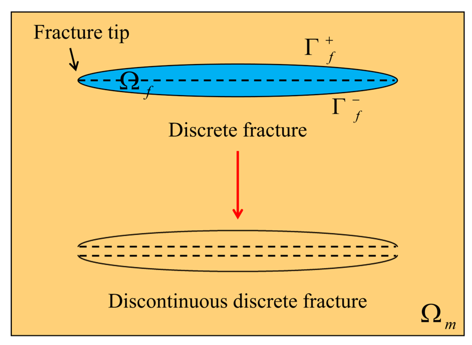
3. Discontinuous Discrete Element Method

The discrete fracture model (DFM) can couple the fluid flow between matrix pores and fractures with high accuracy, but the computational cost increases significantly when the fractures are complex. As shown in Figure 2, the discontinuous discrete fracture model (DDFM) is obtained by optimizing the DFM. While retaining the advantages of the DFM, the effects of fracture surface displacement discontinuity and changes in the properties of the fracture surface crossflow are considered.

3.1. Numerical Description of Fracture–Matrix Coupled Flow

In Figure 2, ${\mathsf{\Omega }}_m$ and ${\mathsf{\Omega }}_f$ are the matrix area and the fracture area, respectively. ${\mathsf{\Gamma }}_f^{+}$ and ${\mathsf{\Gamma }}_f^{-}$ are the upper and lower surfaces of the fracture, respectively. For the initially opened fracture, since its width is much smaller than its length and height, its internal flow can be divided into two parts along the middle interface of the fracture. The crossflow velocity between the upper and lower surfaces of the fracture and the matrix can be expressed as

$$v^{+}={\rho }_{fg}{R}_b\left(p_m-p_f\right)·{\overrightarrow{n}}_f^{+}$$

(19)

$$v^{-}={\rho }_{fg}{R}_b\left(p_m-p_f\right)·{\overrightarrow{n}}_f^{-}$$

(20)

The matrix flow control equation considering the fluid–solid coupling effect can be written as

$${\rho }_{fg}\varphi \left(c_s+Z_p\right){\displaystyle \frac{\partial p}{\partial t}}+{\rho }_{fg}\left(\alpha -\varphi \right){\displaystyle \frac{\partial {\epsilon }_v}{\partial t}}-\nabla ·\left({\rho }_{fg}{Z}_p{D}_e\nabla p\right)=v^{+}·{\overrightarrow{n}}_f^{+}+v^{-}·{\overrightarrow{n}}_f^{-}$$

(21)

From the poroelasticity theory, we know that

$${\displaystyle \frac{\partial {\epsilon }_v}{\partial t}}={\displaystyle \frac{\alpha }{3K}}{\displaystyle \frac{\partial p}{\partial t}}$$

(22)

where $\alpha$ is the effective stress coefficient. $K$ is the bulk modulus of the matrix, MPa.

Substituting Equation (22) into Equation (21), the matrix flow control equation can be written as

$${\rho }_{fg}\left[\varphi \left(c_s+Z_p\right)+{\displaystyle \frac{\alpha \left(\alpha -\varphi \right)}{3K}}\right]{\displaystyle \frac{\partial p}{\partial t}}-\nabla ·\left({\rho }_{fg}{Z}_p{D}_e\nabla p\right)=v^{+}·{\overrightarrow{n}}_f^{+}+v^{-}·{\overrightarrow{n}}_f^{-}$$

(23)

The finite element method is used to solve the model [35].

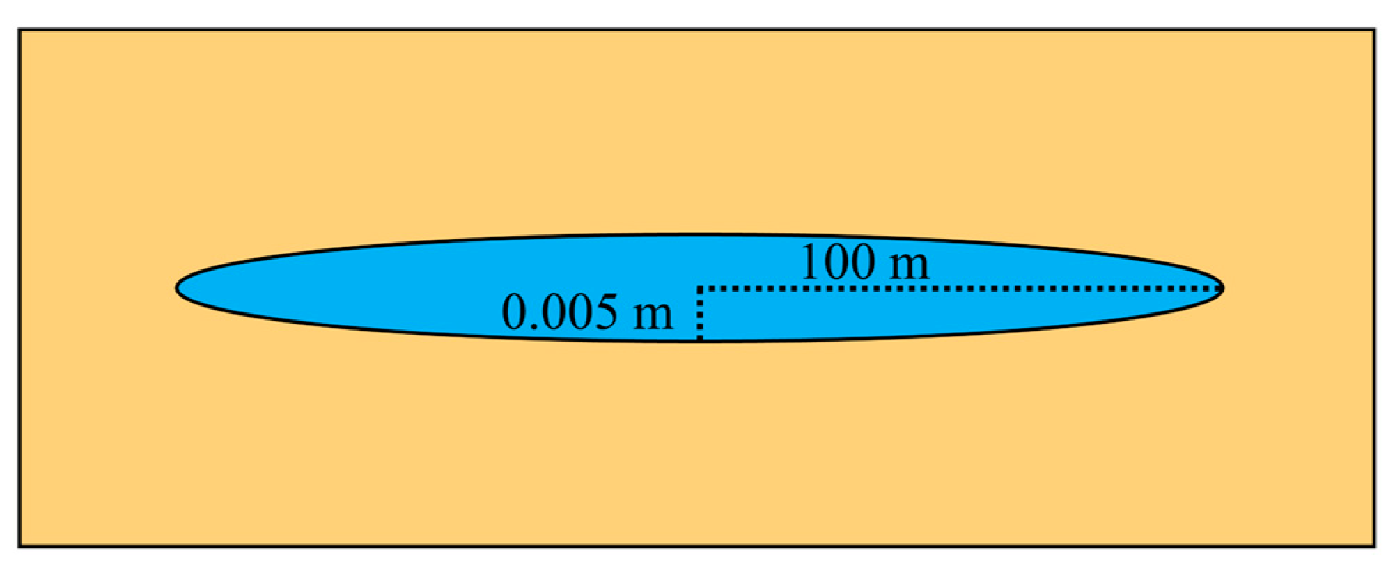
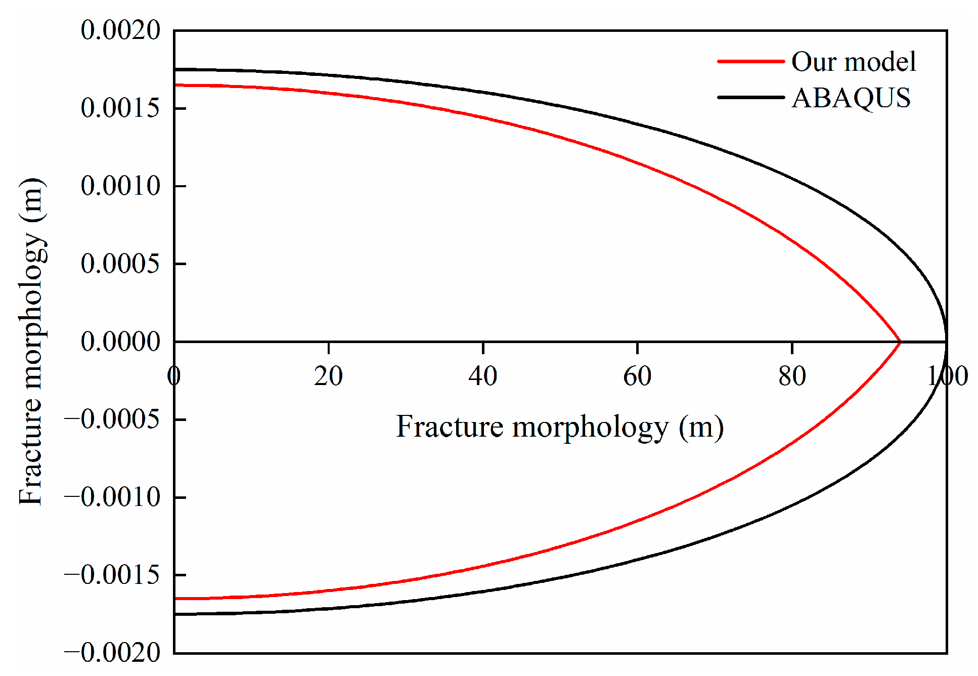
3.2. Model Validation

In order to characterize the true shape of the fracture, considering the crossflow properties of the fracture surface and the discontinuity of displacement, the real fracture model and the DDFM are used to solve a single fracture production process. The real fracture model regards the fracture as a flow space with the same dimensions as the matrix and imposes the same crossflow conditions at the fracture surface. The single fracture geometric model is established as shown in Figure 3. The fracture surface is set as a fixed displacement boundary, and the displacement is calculated using the fracture closure equation through the stress of the fracture surface.

Figure 4 is a comparison of the fracture width changes after simulation with our model and ABAQUS (Abaqus 2023). It can be seen that the fracture closure degree of the discontinuous discrete fracture model is greater. This is because, when the real fracture flow space is established, the fracture space needs to be meshed, and the mesh inside the fracture also has a certain stiffness, which will increase the support effect on the fracture surface. Therefore, the fracture closure width calculated by the real fracture model is smaller than that of the discontinuous discrete fracture model.

4. Results

A random fracture network was established for each fracture in the form of an ellipsoid, and the simulation parameters shown in

Table 1. Simulation parameters.

Simulation Parameters	Values	Units	Symbols
Maximum horizontal principal stress	50	Mpa	$S_H$
Minimum horizontal principal stress	45	Mpa	$S_h$
Initial formation temperature	410	K	$T_0$
Thermal conductivity	3 × 10−11	m2/(s·K)	${\beta }_T$
Interstitial convective heat transfer coefficient	1000	W/(m3·K)	$q_{sf}$
Desorption rate of adsorbed gas	0.8 × 10−5	1/s	$R_d$
Adsorption rate of free gas	0.8 × 10−6	1/s	$R_f$
Effective stress coefficient	0.8	-	$\alpha$
Viscosity coefficient	1 × 1017	Pa·s	$\eta$
Proppant geometric coefficient	2, 4, 6	-	$c$
Proppant elastic modulus	5, 15, 25	GPa	$E_p$
Proppant Poisson’s ratio	0.2, 0.3, 0.4	-	${\nu }_p$
Proppant diameter	0.2, 0.5, 1	mm	$d_p$

were set based on field measured data.

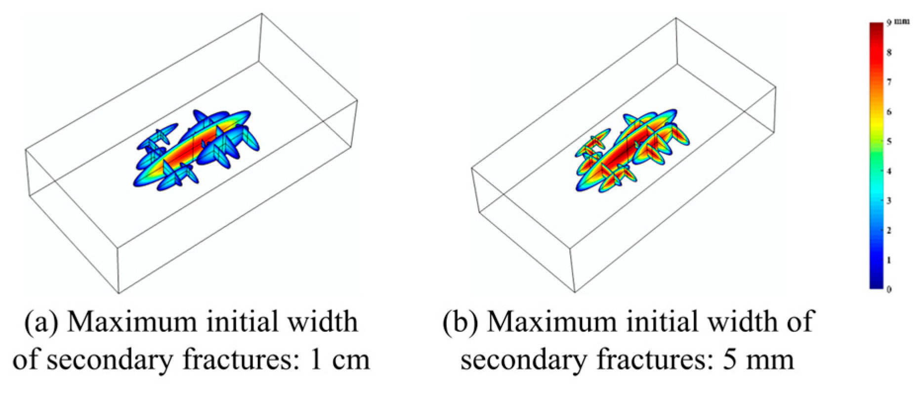
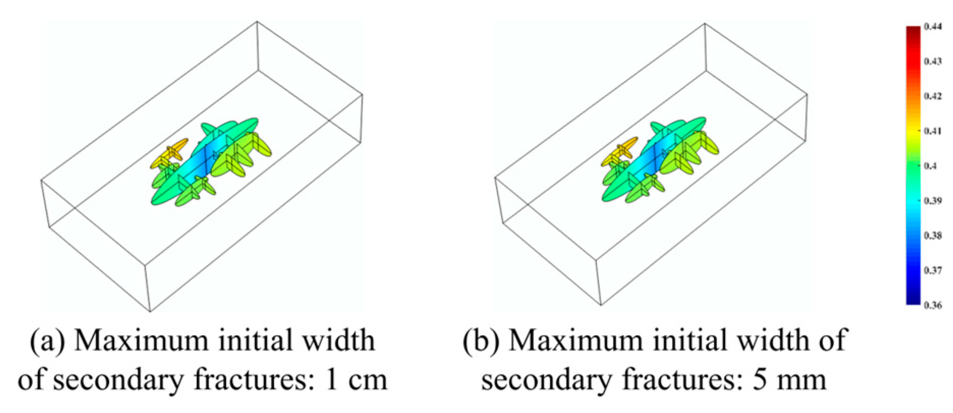
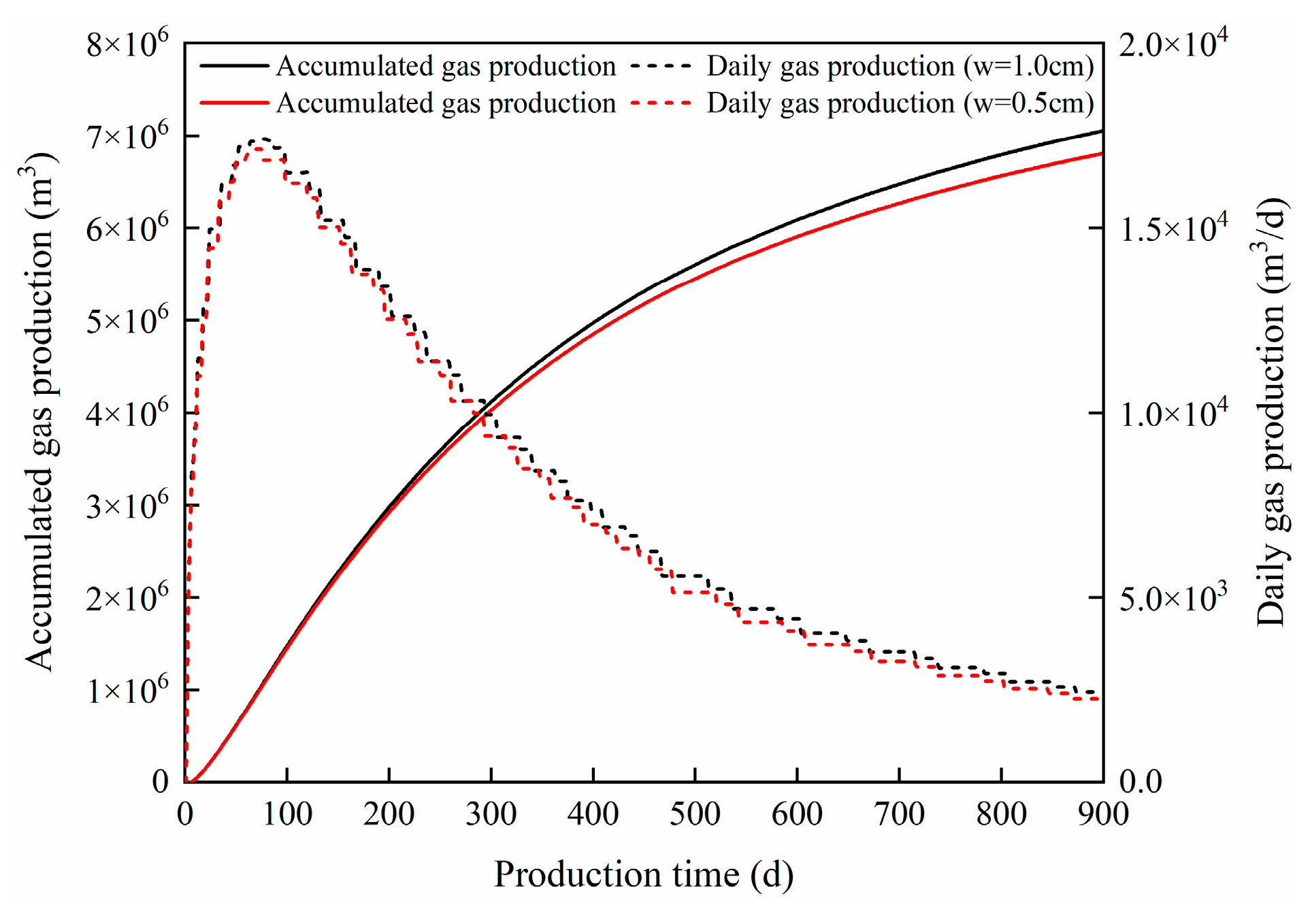
4.1. The Effect of the Proppant Concentration

The greater the proppant concentration, the greater the initial width of the fracture, resulting in more proppant layers in the fracture. In this section, different maximum initial fracture widths are set in the calculation to represent different proppant concentrations. The maximum initial fracture width of the main fracture is twice that of the secondary fracture. As shown in Figure 5, the higher the proppant concentration, the greater the fracture width of the overall fracture network.

As shown in Figure 6, the surface flow properties of the fracture decrease slightly with the increase in the proppant laying concentration. The reason is that, the larger the initial width of the fracture, the higher the deformation energy stored in the fracture surface deformation, which increases the effective closing stress of the fracture surface, thereby increasing the embedding of the proppant in the fracture surface.

As shown in the gas production curve of Figure 7, increasing the proppant concentration to improve the fracture width (or conductivity) has no significant effect on shale gas production. When the initial fracture width increases from 5 mm to 1 cm, the cumulative gas production in 900 days only increases by 3.65%. Although the increase in proppant laying concentration maintains a larger fracture conductivity and drainage area, the increase in fracture width increases the fracture gas transportation capacity, thereby reducing the average gas pressure in the fracture, but increases the embedding amount of proppant, which reduces the crossflow coefficient of the fracture surface. After comprehensive consideration, the gas supply rate of the matrix to the fracture does not increase significantly with the increase in the fracture width. Therefore, although increasing the proppant laying concentration will reduce the degree of fracture closure and increase the fracture conductivity, blindly improving the fracture conductivity will not effectively increase shale gas production.

4.2. The Effect of Proppant Placement

The geometric coefficient is introduced to characterize the degree of proppant placement in the fracture. The larger the proppant placement geometric coefficient, the more uneven the proppant is placed on the fracture surface—that is, the worse the proppant placement is, which means that more fracture surfaces are not supported. Taking the three cases of proppant geometric coefficients of 2, 4 and 6, it means that only 1/2, 1/4 and 1/6 of the fracture surface area are effectively supported by the proppant, respectively. As shown in Figure 8, the larger the proppant placement geometric coefficient, the significantly smaller the fracture width. Since the area of the fracture surface blocked by proppant decreases with the increase of the proppant placement geometric coefficient, the crossflow coefficient of the unclosed fracture surface increases with the increase of the proppant placement geometric coefficient, as shown in Figure 9.

As shown in the gas production curve in Figure 10, shale gas production decreases significantly with the increase in the proppant placement geometric coefficient. When the proppant placement geometric coefficient increases from 2 to 4 and 6, the three-year cumulative gas production decreases by 40.9% and 98.6%, respectively. The degree of proppant placement determines whether it can effectively support the fracture surface, which is crucial to maintaining the fracture conductivity and effective drainage area and has a significant impact on shale gas production.

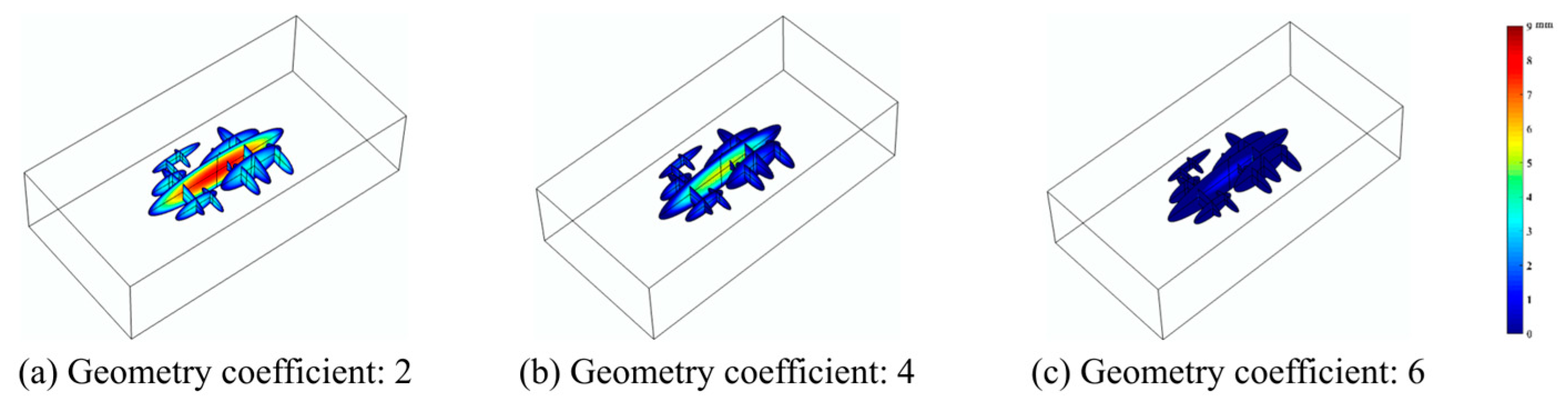
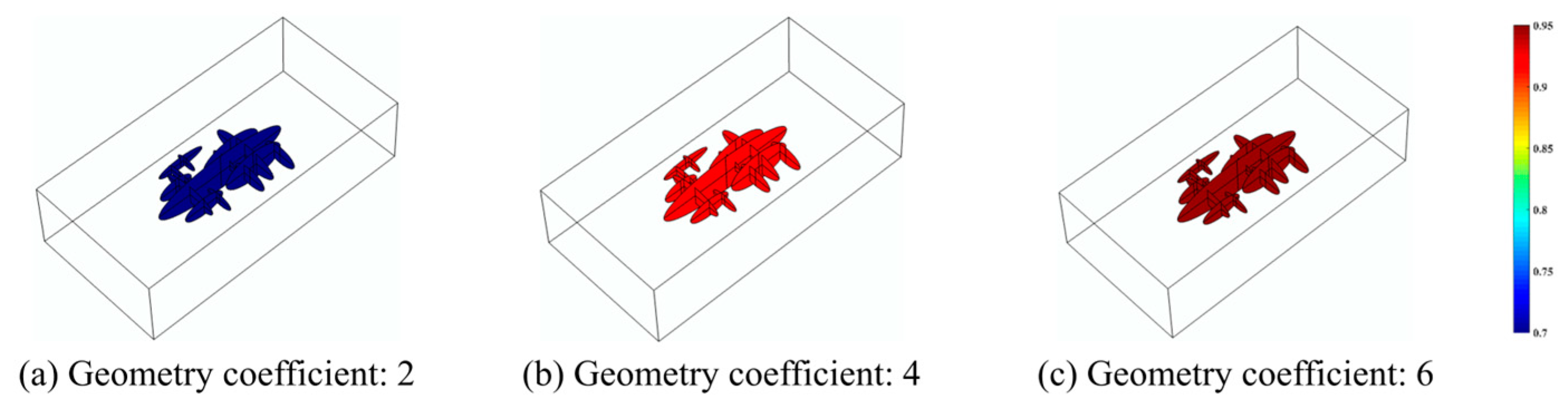
4.3. The Effect of Proppant Mechanical Properties

It can be seen from Figure 11 that the fracture width increases with the increase of the elastic modulus of the proppant. Since the elastic deformation of the proppant layer decreases with the increase of its elastic modulus, and there are more proppant layers in the main fracture than in the secondary fracture, the effect of the elastic modulus of the proppant on the change of the width of the main fracture is more obvious than that of the secondary fracture. It can be seen from Figure 12 that the change of the Poisson’s ratio of the proppant has little effect on the fracture width.

Figure 13 shows the effect of the proppant elastic modulus on the crossflow properties of the fracture surface. It can be seen that, with the increase of the proppant elastic modulus, the crossflow coefficient of the fracture surface decreases significantly. The reason is that, the larger the proppant elastic modulus, the harder it is, which increases the embedding amount of proppant on the fracture surface, blocking the pores on the fracture surface and thereby reducing the crossflow coefficient of the fracture surface. Figure 14 shows the effect of the proppant Poisson’s ratio on the crossflow properties of the fracture surface. It can be seen that, with the increase of the proppant Poisson’s ratio, the crossflow coefficient of the fracture surface decreases slightly. The reason is that, the larger the proppant Poisson’s ratio, the greater the lateral deformation caused by the vertical deformation of the proppant under the closing stress, which increases the shielding degree of the proppant on the fracture surface, thereby reducing the crossflow coefficient of the fracture surface.

As can be seen from the gas production curve in Figure 15, the cumulative gas production increases with the increase of the proppant elastic modulus, but when the proppant elastic modulus increases from 5 GPa to 15 GPa and 25 GPa, the cumulative gas production after 900 days of production only increases by 2.5% and 3.1%. This shows that the elastic modulus of the proppant has a significant effect on fracture closure, but the proppant with a larger elastic modulus increases the embedding amount of the proppant in the fracture surface while maintaining higher fracture conductivity and a larger drainage area, thereby reducing the crossflow capacity of the fracture surface. Under comprehensive consideration, the change of the proppant elastic modulus has little effect on shale gas production. Although the increase in the proppant Poisson’s ratio can better maintain the fracture drainage capacity during the production process, the crossflow capacity of the fracture surface is reduced. After combining the influence of the two factors, the proppant Poisson’s ratio has little effect on shale gas production, as shown in Figure 16.

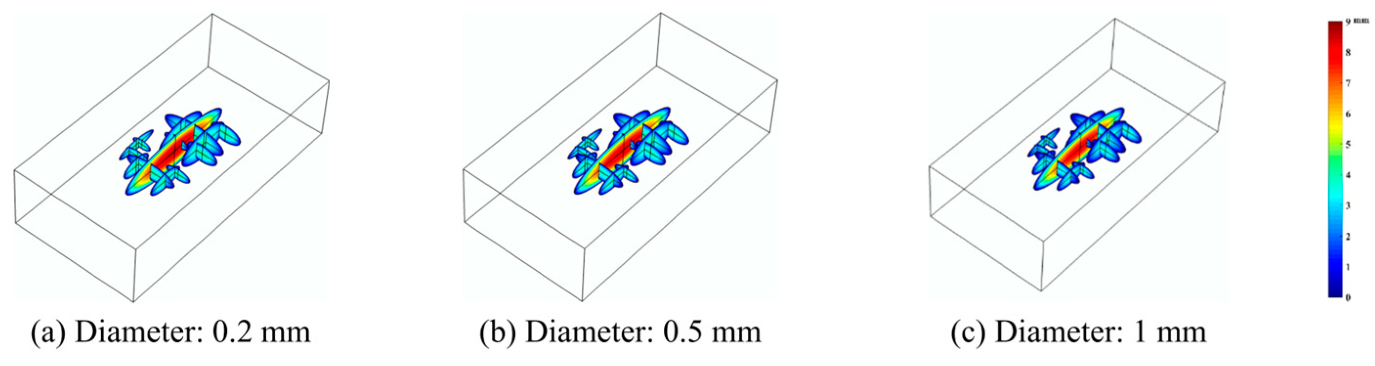
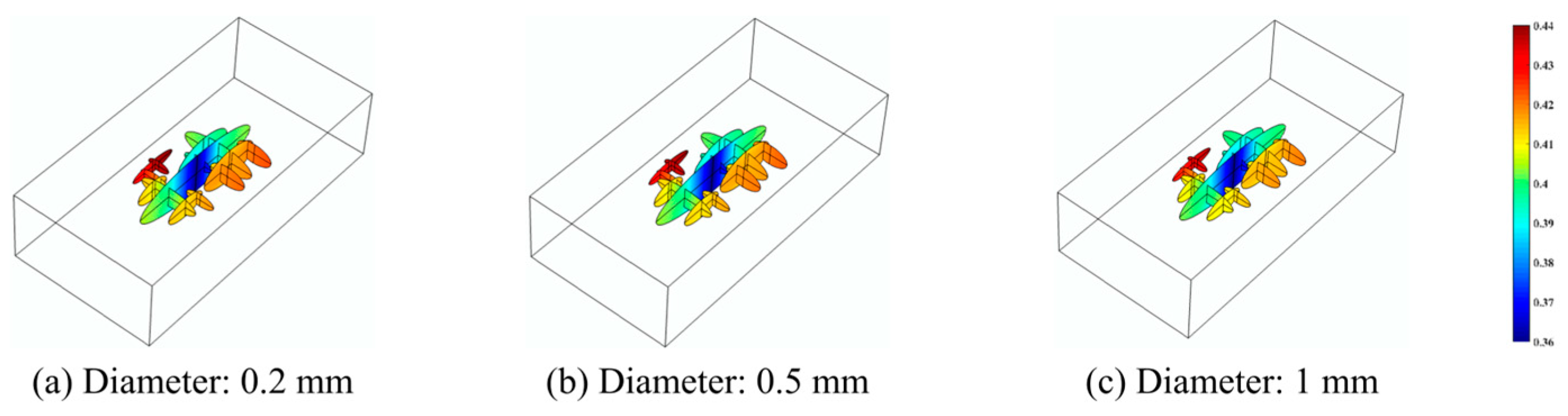
4.4. The Effect of the Proppant Diameter

The same number of proppant layers is set, and the proppant diameter is changed. Therefore, the smaller the proppant diameter, the smaller the initial width of the fracture and the lower the construction cost. As shown in Figure 17, as the proppant diameter increases, the fracture width decreases.

As shown in Figure 18, the fracture surface crossflow coefficient decreases with the increase of the proppant diameter, which is more obvious for secondary fractures. This also shows that a small-sized proppant is more suitable for complex fracture networks.

As shown in Figure 19, the smaller the proppant diameter, the greater the shale gas production. When the proppant diameter is reduced from 1 mm to 0.5 mm and 0.2 mm, the cumulative gas production in 900 days of production increases by 2% and 5.5% respectively. Since the proppant laying concentration corresponding to the small-sized proppant is lower, the construction cost is also lower, and the small-sized proppant is easier to pump into the secondary fracture network; the actual construction effect will also be better than the large-sized proppant. Therefore, the small-sized proppant is more suitable for deep shale gas hydraulic fracturing construction.

5. Conclusions

This paper establishes a fluid–solid–thermal coupling model in the fracture closure process and solves it using the DDFM. The influence of factors such as proppant concentration, proppant placement, proppant mechanical properties and proppant diameter are analyzed by analyzing the change law of shale gas production. The simulation results show that:

(1)

The fracture closure width calculated by the real fracture model is smaller than that of the discontinuous discrete fracture model. However, the applicability of the model to ultra-deep shale gas reservoirs needs further verification, and the impact of extreme geological conditions (such as high-stress anisotropy) is not considered.

(2)

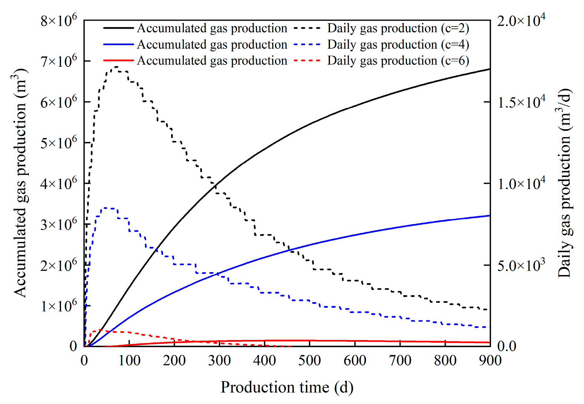
The higher the proppant concentration, the wider the fractures formed, but it did not have a significant impact on shale gas production. When the initial fracture width increased from 5 mm to 1 cm, the cumulative gas production over 900 days increased by only 3.65%.

(3)

Poor proppant placement means that the proppant is unevenly placed in the fracture. At this time, the proppant cannot effectively support the fracture surface, resulting in a decrease in conductivity and effective drainage area and a significant decrease in shale gas production.

(4)

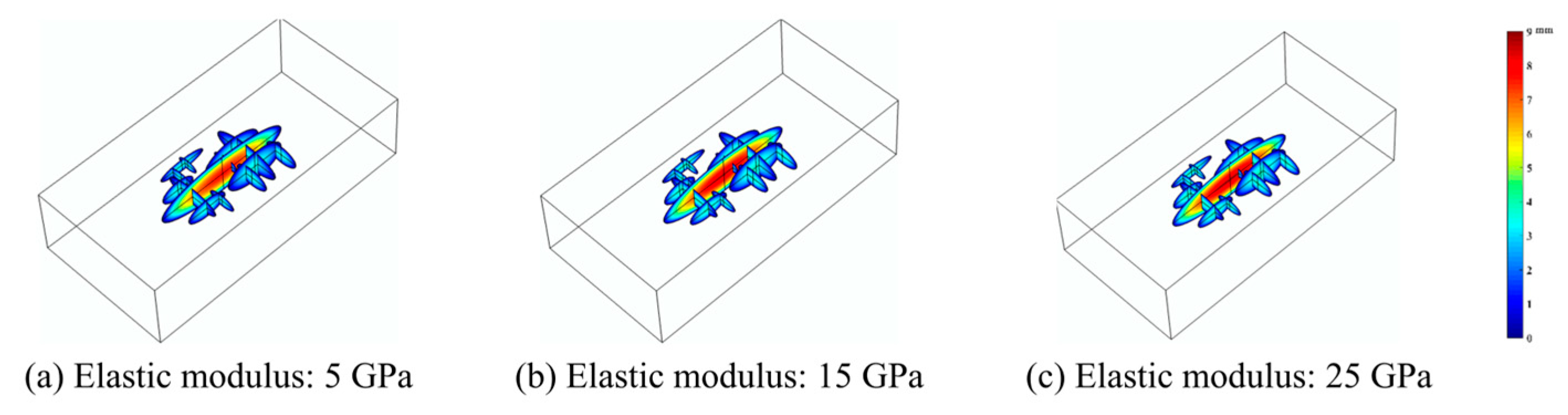
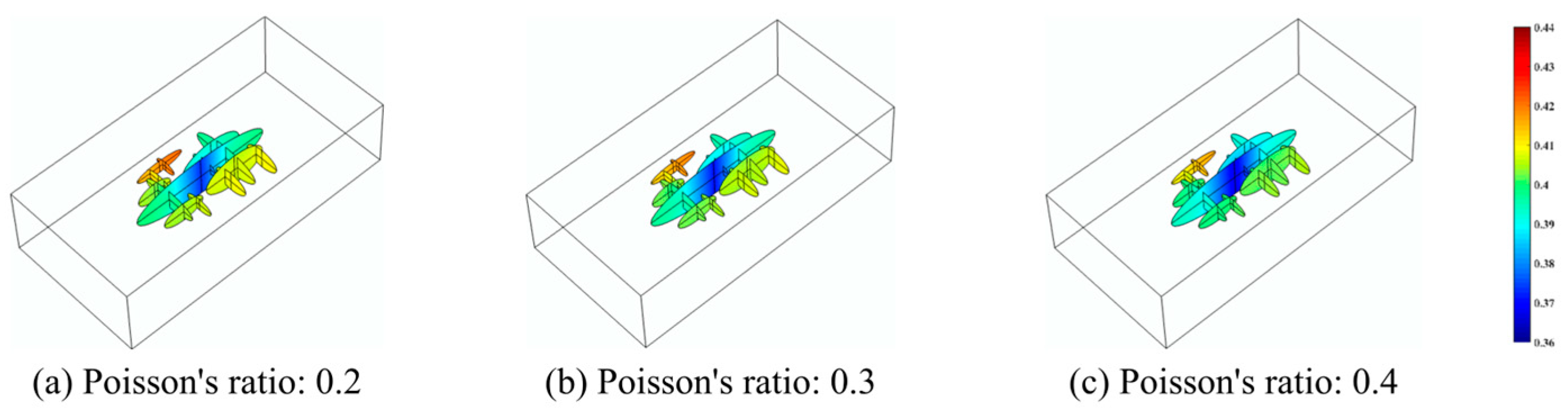
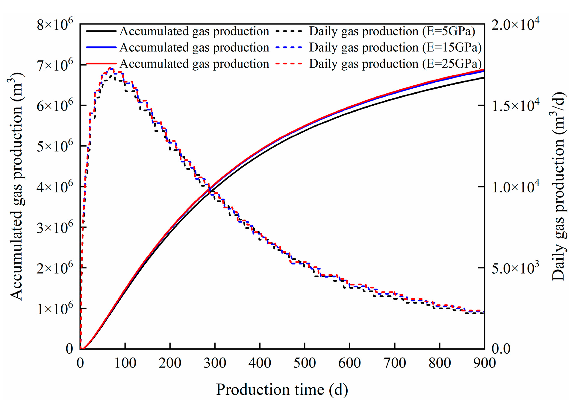
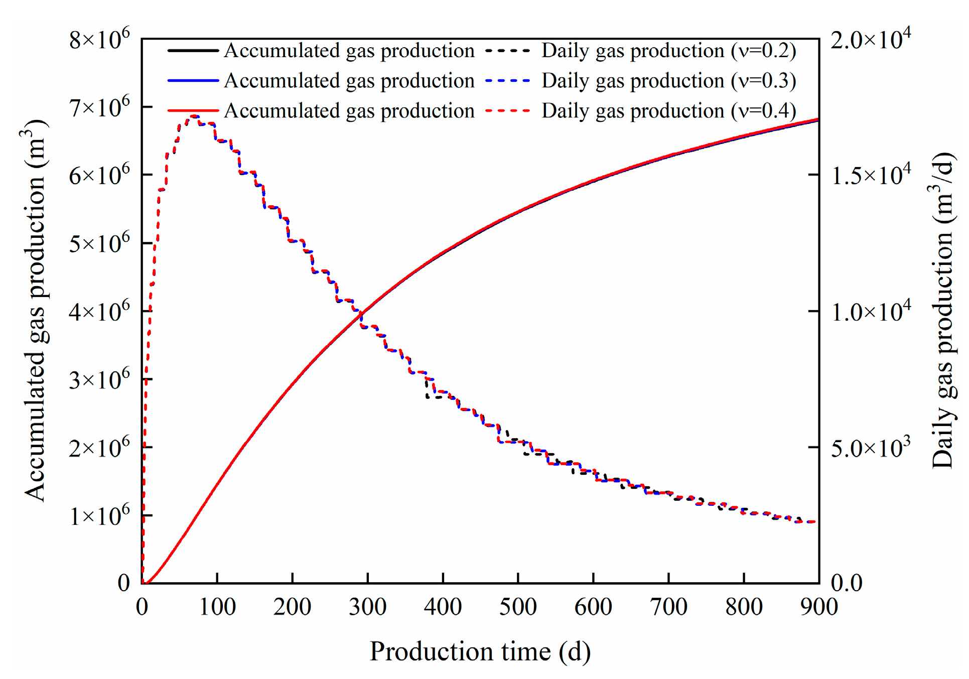
When the elastic modulus of the proppant increases, the fracture width and cumulative gas production increase accordingly, but the proppant with a larger elastic modulus increases the embedding amount, resulting in a poor fracture transformation effect. Although the increase in the Poisson’s ratio of the proppant increases the leakage area, it reduces the crossflow capacity, so the Poisson’s ratio of the proppant has little effect on shale gas production.

(5)

Small-sized proppants have a lower proppant laying concentration, which brings lower construction costs. Small-sized proppants are easier to pump to the far end of the fracture network, and the actual construction effect will be better than large-sized proppants. Therefore, small-sized proppants are more suitable for deep shale gas hydraulic fracturing construction.

References

1. Sun, C.; Nie, H.; Dang, W.; Chen, Q.; Zhang, G.; Li, W.; Lu, Z. Shale gas exploration and development in China: Current status, geological challenges, and future directions. Energy Fuels 2021, 35, 6359–6379. [Google Scholar] [CrossRef]
2. Zhao, W.; Jia, A.; Wei, Y.; Wang, J.; Zhu, H. Progress in shale gas exploration in China and prospects for future development. China Pet. Explor. 2020, 25, 31. [Google Scholar] [CrossRef]
3. Ma, X.; Wang, H.; Zhou, S.; Shi, Z.; Zhang, L. Deep shale gas in China: Geological characteristics and development strategies. Energy Rep. 2021, 7, 1903–1914. [Google Scholar] [CrossRef]
4. Jiang, T.; Bian, X.; Wang, H.; Li, S.; Jia, C.; Liu, H.; Sun, H. Volume fracturing of deep shale gas horizontal wells. Nat. Gas Ind. B 2017, 4, 127–133. [Google Scholar] [CrossRef]
5. Zhao, J.; Ren, L.; Jiang, T.; Hu, D.; Wu, L.; Wu, J.; Yin, C.; Li, Y.; Hu, Y.; Lin, R.; et al. Ten years of gas shale fracturing in China: Review and prospect. Nat. Gas Ind. B 2022, 9, 158–175. [Google Scholar] [CrossRef]
6. Wang, H.; Chen, L.; Qu, Z.; Yin, Y.; Kang, Q.; Yu, B.; Tao, W. Modeling of multi-scale transport phenomena in shale gas production-A critical review. Appl. Energy 2020, 262, 114575. [Google Scholar] [CrossRef]
7. Zhang, L.; Shan, B.; Zhao, Y.; Guo, Z. Review of micro seepage mechanisms in shale gas reservoirs. Int. J. Heat Mass Transf. 2019, 139, 144–179. [Google Scholar] [CrossRef]
8. Zhang, T.; Sun, S.; Song, H. Flow mechanism and simulation approaches for shale gas reservoirs: A review. Transp. Porous Media 2019, 126, 655–681. [Google Scholar] [CrossRef]
9. Darcy, H. Les Fontaines Publiques de la Ville de Dijon: Exposition et Aapplication des Principes à Suivre et des Formules à Employer dans les Questions de Distribution D’eau; Victor dalmont: Paris, France, 1856. [Google Scholar]
10. Xiong, X.; Devegowda, D.; Michel, G.G.; Sigal, R.F.; Civan, F. A Fully-Coupled Free and Adsorptive Phase Transport Model for Shale Gas Reservoirs Including Non-Darcy Flow Effects. In Proceedings of the SPE Annual Technical Conference and Exhibition, San Antonio, TX, USA, 8–10 October 2012. [Google Scholar] [CrossRef]
11. Berkowitz, B.; Ewing, R.P. Percolation theory and network modeling applications in soil physics. Surv. Geophys. 1998, 19, 23–72. [Google Scholar] [CrossRef]
12. Javadpour, F.; Fisher, D.; Unsworth, M. Nanoscale gas flow in shale gas sediments. J. Can. Pet. Technol. 2007, 46, PETSOC-07-10-06. [Google Scholar] [CrossRef]
13. Javadpour, F. Nanopores and apparent permeability of gas flow in mudrocks (shales and siltstone). J. Can. Pet. Technol. 2009, 48, 16–21. [Google Scholar] [CrossRef]
14. Fathi, E.; Akkutlu, I.Y. Matrix heterogeneity effects on gas transport and adsorption in coalbed and shale gas reservoirs. Transp. Porous Media 2009, 80, 281–304. [Google Scholar] [CrossRef]
15. Fathi, E.; Akkutlu, I.Y. Mass transport of adsorbed-phase in stochastic porous medium with fluctuating porosity field and nonlinear gas adsorption kinetics. Transp. Porous Media 2012, 91, 5–33. [Google Scholar] [CrossRef]
16. Zhang, Q.; Su, Y.; Wang, W.; Lu, M.; Sheng, G. Gas transport behaviors in shale nanopores based on multiple mechanisms and macroscale modeling. Int. J. Heat Mass Transf. 2018, 125, 845–857. [Google Scholar] [CrossRef]
17. Zhang, L.; Li, D.; Lu, D.; Zhang, T. A new formulation of apparent permeability for gas transport in shale. J. Nat. Gas Sci. Eng. 2015, 23, 221–226. [Google Scholar] [CrossRef]
18. Liang, Y.; Cheng, Y.; Han, Z.; Pidho, J.J.; Yan, C. Study on multiscale fluid–solid coupling theoretical model and productivity analysis of horizontal well in shale gas reservoirs. Energy Fuels 2023, 37, 5059–5077. [Google Scholar] [CrossRef]
19. Song, F.; Hu, X.; Ji, K.; Huang, X. Effect of fluid-solid coupling on shale mechanics and seepage laws. Nat. Gas Ind. B 2018, 5, 41–47. [Google Scholar] [CrossRef]
20. Wu, Y.S.; Pruess, K. A multiple-porosity method for simulation of naturally fractured petroleum reservoirs. SPE Reserv. Eng. 1988, 3, 327–336. [Google Scholar] [CrossRef]
21. Kim, J.G.; Deo, M.D. Finite element, discrete-fracture model for multiphase flow in porous media. AIChE J. 2000, 46, 1120–1130. [Google Scholar] [CrossRef]
22. Wei, S.; Xia, Y.; Jin, Y.; Chen, M.; Chen, K. Quantitative study in shale gas behaviors using a coupled triple-continuum and discrete fracture model. J. Pet. Sci. Eng. 2019, 174, 49–69. [Google Scholar] [CrossRef]
23. Danso, D.K.; Negash, B.M.; Ahmed, T.Y.; Yekeen, N.; Ganat, T.A.O. Recent advances in multifunctional proppant technology and increased well output with micro and nano proppants. J. Pet. Sci. Eng. 2021, 196, 108026. [Google Scholar] [CrossRef]
24. Katende, A.; O’Connell, L.; Rich, A.; Rutqvist, J.; Radonjic, M. A comprehensive review of proppant embedment in shale reservoirs: Experimentation, modeling and future prospects. J. Nat. Gas Sci. Eng. 2021, 95, 104143. [Google Scholar] [CrossRef]
25. Yan, X.; Huang, Z.; Zhang, Q.; Fan, D.; Yao, J. Numerical investigation of the effect of partially propped fracture closure on gas production in fractured shale reservoirs. Energies 2020, 13, 5339. [Google Scholar] [CrossRef]
26. Li, K.; Gao, Y.; Lyu, Y.; Wang, M. New mathematical models for calculating proppant embedment and fracture conductivity. SPE J. 2015, 20, 496–507. [Google Scholar] [CrossRef]
27. Kim, J.; Seo, Y.; Wang, J.; Lee, Y. History matching and forecast of shale gas production considering hydraulic fracture closure. Energies 2019, 12, 1634. [Google Scholar] [CrossRef]
28. Zheng, S.; Manchanda, R.; Sharma, M.M. Modeling fracture closure with proppant settling and embedment during shut-in and production. SPE Drill. Complet. 2020, 35, 668–683. [Google Scholar] [CrossRef]
29. Zhang, F.; Emami-Meybodi, H. Flowback fracture closure of multi-fractured horizontal wells in shale gas reservoirs. J. Pet. Sci. Eng. 2020, 186, 106711. [Google Scholar] [CrossRef]
30. Pati, S.; Borah, A.; Boruah, M.P.; Randive, P.R. Critical review on local thermal equilibrium and local thermal non-equilibrium approaches for the analysis of forced convective flow through porous media. Int. Commun. Heat Mass Transf. 2022, 132, 105889. [Google Scholar] [CrossRef]
31. Xia, Y.; Wei, S.; Jin, Y.; Chen, K. Self-diffusion flow and heat coupling model applicable to the production simulation and prediction of deep shale gas wells. Nat. Gas Ind. B 2021, 8, 359–366. [Google Scholar] [CrossRef]
32. Liang, Z.; Chen, Z.; Rahman, S.S. Experimental investigation of the primary and secondary creep behaviour of shale gas reservoir rocks from deep sections of the Cooper Basin. J. Nat. Gas Sci. Eng. 2020, 73, 103044. [Google Scholar] [CrossRef]
33. Findley, W.N.; Davis, F.A. Creep and Relaxation of Nonlinear Viscoelastic Materials; Courier Corporation: New York, NY, USA, 2013; ISBN 0-486-66016-8. [Google Scholar]
34. Hertz, H. Ueber die Berührung fester elastischer Körper. J. Reine Angew. Math. 1882, 1882, 156–171. [Google Scholar] [CrossRef]
35. Wei, S. The Thermo-Hydro-Mechanical Couplingmechanism of Fracture Closure During Deepshale Gas Production. Doctoral Dissertation, China University of Petroleum, Beijing, China, 2022. [Google Scholar] [CrossRef]
Figure 1. Changes caused by fracture closure.
Applsci 15 02365 g001
Figure 2. DFM and DDFM.
Applsci 15 02365 g002
Figure 3. Fracture model.
Applsci 15 02365 g003
Figure 4. Comparison of fracture widths between our model and ABAQUS.
Applsci 15 02365 g004
Figure 5. Effect of proppant concentration on the fracture width.
Applsci 15 02365 g005
Figure 6. Effect of proppant concentration on the dimensionless fracture surface crossflow coefficient.
Applsci 15 02365 g006
Figure 7. Effect of proppant concentration on shale gas production.
Applsci 15 02365 g007
Figure 8. Effect of proppant placement on the fracture width.
Applsci 15 02365 g008
Figure 9. Effect of proppant placement on the dimensionless fracture surface crossflow coefficient.
Applsci 15 02365 g009
Figure 10. Effect of proppant placement on shale gas production.
Applsci 15 02365 g010
Figure 11. Effect of the proppant elastic modulus on the fracture width.
Applsci 15 02365 g011
Figure 12. Effect of the proppant Poisson’s ratio on the fracture width.
Applsci 15 02365 g012
Figure 13. Effect of the proppant elastic modulus on the dimensionless fracture surface crossflow coefficient.
Applsci 15 02365 g013
Figure 14. Effect of the proppant Poisson’s ratio on the dimensionless fracture surface crossflow coefficient.
Applsci 15 02365 g014
Figure 15. Effect of the proppant elastic modulus on shale gas production.
Applsci 15 02365 g015
Figure 16. Effect of the proppant Poisson’s ratio on shale gas production.
Applsci 15 02365 g016
Figure 17. Effect of the proppant diameter on the fracture width.
Applsci 15 02365 g017
Figure 18. Effect of the proppant diameter on the dimensionless fracture surface crossflow coefficient.
Applsci 15 02365 g018
Figure 19. Effect of the proppant diameter on shale gas production.
Applsci 15 02365 g019