Deep-Radiomic Fusion for Early Detection of Pancreatic Ductal Adenocarcinoma

Abstract

Leveraging the complementary strengths of handcrafted radiomics and data-driven deep learning, this work develops and rigorously benchmarks three modeling streams (Models A, B and C) for pancreatic ductal adenocarcinoma (PDAC) detection on multiphase abdominal Computed Tomography (CT) scans. Model A distills hundreds of PyRadiomics descriptors to sixteen interpretable features that feed a gradient-boosted machine learning model, achieving discrimination (external AUC ≈ 0.99) with excellent calibration. Model B adopts a 3-D CBAM-ResNet-18 trained under weighted cross-entropy and mixed precision; although less accurate in isolation, it yields volumetric Grad-CAM maps that localize the tumor and provide explainability. Model C explores two fusion strategies that merge radiomics and deep embeddings: (i) a two-stage “frozen-stream” variant that locks both feature extractors and learns only a lightweight gating block plus classifier, and (ii) a full end-to-end version that allows the CNN’s adaptor layer to co-train with the fusion head. The frozen approach surpasses the single stream, whereas the end-to-end model reports external AUC of 0.987, balanced sensitivity/specificity above 0.93, and a Brier score below 0.05, while preserving clear Grad-CAM alignment with radiologist-drawn masks. Results demonstrate that a carefully engineered deep-radiomic fusion pipeline can deliver accurate, well-calibrated and interpretable PDAC triage directly from routine CT. Our contributions include a stability-verified 16-feature radiomic signature, a novel deep-radiomic fusion design that improves robustness and interpretability across vendors and a fully guideline-aligned, openly released pipeline for reproducible PDAC detection on routine CT.

1. Introduction

Pancreatic cancer (Pancreatic ductal adenocarcinoma, PDAC) ranks as the third leading cause of cancer-related mortality across both sexes [1]. As pancreatic malignant tumors are aggressive, the 5-year survival rate is hovering at around 5–10%. Such dire statistics are largely attributed to poor prognosis and limited treatment options [1]. Early detection is critical for improving patient outcomes, as the only curative therapeutic option is surgical resection. Given the aggressive nature of PDAC, many tumors get diagnosed at an advanced stage, where surgical resection is not possible or tumor metastasis has already taken place [2]. Consequently, there is a pressing need for innovative methods to enhance diagnostic accuracy and increase early detection [3].

Radiomics has emerged as a promising field that capitalizes on advanced image analysis to quantify tumor phenotypes [4]. Originally developed as a way to mine high-dimensional data from standard medical images, radiomics allows researchers and clinicians to extract and interpret complex textural, shape-based, and intensity-based features [5]. In pancreatic cancer, radiomic techniques have shown potential in discriminating between malignant and benign lesions, predicting treatment response, and stratifying patient prognosis. By transforming medical images into a dataset of quantifiable metrics, radiomics holds the promise of uncovering imaging biomarkers that can guide personalized clinical decision-making [6].

Parallel to the rise in radiomics, the field of artificial intelligence (AI) has experienced rapid growth, particularly with the advent of deep learning approaches. Deep learning, rooted in neural networks capable of automatically learning feature representations, has revolutionized image-based tasks in medical applications [7]. From detecting microcalcifications in mammograms to segmenting brain tumors in MRI scans, AI-driven models, especially convolutional neural networks (CNNs), have demonstrated human-level performance in various diagnostic contexts. When applied to PDAC, these systems aim to identify early signs of neoplasia and differentiate subtle morphological patterns that may be challenging for human observers to detect [8].

An emerging and increasingly explored concept is the combination of radiomics with deep learning, referred to as “deep radiomics” [9]. The rationale behind this integration is clear: while radiomics provides handcrafted, interpretable features that reflect known statistical or geometric properties, deep learning can uncover latent patterns and relationships directly from the data without explicit feature engineering. By merging these complementary approaches, researchers hope to maximize predictive performance, improve model robustness, and expand the range of discovered imaging biomarkers. This synergistic strategy could enhance early pancreatic cancer detection, refine prognostic assessments, and facilitate the development of adaptive treatment protocols [10].

To this end, this work introduces and benchmarks three complementary modeling streams for PDAC detection from multiphase abdominal CT scans. Model A extracts and filters hundreds of PyRadiomics features down to a core set of 16 interpretable descriptors powering a gradient-boosted machine. Model B employs a 3D CBAM-ResNet-18 trained with weighted cross-entropy and mixed precision, additionally providing volumetric Grad-CAM explainability. Model C integrates both modalities via two fusion strategies: (i) a frozen-stream architecture that locks feature extractors and trains a lightweight fusion block (Model C1), and (ii) an end-to-end variant enabling joint optimization of the CNN adaptor and fusion head (Model C2). Key innovations of the present work can be summarized in the following points:

• Introduction of a hybrid stream design that combines explicit feature selection with attention-based CNNs.
• Presentation of an efficient training pipeline that separates backbone training from fusion fine-tuning.
• Robust evaluation process incorporating classical metrics along with calibration curves and voxel-level heatmaps to enhance clinical interpretability.
• Introduction of a cross-vendor validation approach by assessing generalizability on scans from different CT vendors.
• Comprehensive adherence to and demonstration of community-endorsed best practices, including the Checklist for Evaluation of Radiomics (CLEAR), AI-Ready Imaging Standards for Evaluation (ARISE), European Society of Radiology (ESR) Essentials, Transparent Reporting of a multivariable prediction model for Individual Prognosis Or Diagnosis—Artificial Intelligence extension (TRIPOD-AI), Findable-Accessible-Interoperable-Reusable principles (FAIR), the Checklist for Artificial Intelligence in Medical Imaging (CLAIM), the METhodological RadiomICs Score (METRICS) and the Radiomics Quality Score (RQS) guidelines, through transparent data sharing, open code, rigorous validation and full explainability.

Related Work and Contribution

Dmitriev et al. (2017) [11] proposed a hybrid radiomics and deep learning model for pancreatic cyst classification, applying a Random Forest (RF) with 14 quantitative radiomic features (patient demographics, lesion shape, intensities) alongside a 2D CNN for higher-level feature extraction in contrast-enhanced CT. They fused both models via Bayesian ensemble, achieving an overall accuracy of 83.6% across 134 patients with four different pancreatic lesions and tumors (Intraductal Papillary Mucinous Neoplasms (IPMNs), Mucinous Cystic Neoplasms (MCNs), Serous Cystadenomas (SCAs), and Solid Pseudopapillary Neoplasms (SPNs)). Notably, the RF excelled at smaller cysts, while the CNN performed better in characterizing larger lesions. Ziegelmayer et al. (2020) [12] similarly integrated handcrafted radiomics from PyRadiomics (1411 features) and VGG19-based deep features (256) to differentiate PDAC from autoimmune pancreatitis (AIP) in 86 portal-phase CTs. Deep features yielded an AUC of 0.90 (89% sensitivity, 83% specificity), outperforming radiomics alone, reporting an AUC of 0.80. Although the authors operated on each feature set separately rather than fusing them, CNN-derived activations captured more nuanced patterns than traditional radiomics, highlighting the benefit of deep learning in challenging differential diagnoses.

Zhang et al. (2021) [13] explored a fusion approach for PDAC survival prediction in 98 contrast-enhanced CTs (68 training, 30 validation). They extracted 1428 handcrafted features (PyRadiomics) along with 35 transfer learning-based deep features (LungTrans CNN). Testing multiple fusion schemes (PCA, Boruta, Cox, and LASSO), they ultimately introduced a novel risk score method that combines radiomics and deep feature random forests, achieving an AUC of 0.84—notably better than traditional methods. Wei et al. (2023) [14] took a multimodal path, fusing radiomics and deep learning features from 18F-FDG PET/CT to distinguish PDAC (n = 64) from AIP (n = 48). Radiomics captured histogram, texture, and morphology from both PET and CT, while a VGG11 CNN model was employed to extract high-level features. Their multidomain fusion model (MF_model) reached an AUC of 0.964, outperforming the radiomics-only (89.5%) and deep-only (93.6%) approaches.

Yao et al. (2023) [15] applied a multi-institutional MRI pipeline for intraductal papillary mucinous neoplasm (IPMN) risk stratification, assembling 246 T1-/T2-weighted MRI scans from five centers. After nnUNet-based pancreas segmentation, 107 radiomics features were extracted and combined with deep features from five CNN architectures (DenseNet, ResNet18, AlexNet, MobileNet, and ViT), including clinical factors. Their weighted-averaging fusion significantly boosted accuracy from 61.3 to 71.6% (single CNN/radiomics) to 81.9%. Vétil et al. (2023) [16] introduced a mutual-information-minimized (MI) fusion approach for early PDAC detection using 2319 and 1094 CT scans for training and testing, respectively. Handcrafted radiomics (PyRadiomics) were paired with deep features from a Variational Autoencoder (VAE), but critically, the VAE was trained to minimize redundant information relative to the handcrafted feature space. This MI-based technique boosted AUC by ~1.13% over handcrafted alone.

Finally, Gu et al. (2025) [17] presented a multiscale CT “deep-learning radiomics” nomogram to predict recurrence-free survival after PDAC resection in 469 patients across four centers. The authors extracted 1688 intratumoural and peritumoural radiomics features and 2048 deep features from a transfer-learned ResNet-50 on optimally sized 2-D crops. Three image signatures (intratumoural radiomics, 4 mm peritumoural radiomics, deep features) plus Cancer Antigen (CA) 19-9 were combined via Cox regression into a nomogram. In external validation, the model achieved C-indices of 0.70–0.78 (versus 0.54–0.57 for American Joint Committee on Cancer (AJCC)), with time-dependent AUCs up to 0.97 at one year. Peritumoural radiomics and larger-context deep features provided complementary prognostic value, though retrospective design and scanner heterogeneity remained limitations.

Compared to the aforementioned related work, the proposed pipeline, across all four experiments (Models A, B, C {C1, C2}), consistently outperformed or matched the best figures reported in the recent fusion literature, but more importantly did so with a design that is simpler to train, easier to interpret and demonstrably more robust when scanners change. More specifically:

• First, the purely hand-crafted route (Model A, 16 PyRadiomics features + SVM) already sets a very high baseline: internal AUC = 0.997 and external AUC = 0.991 out-strip the 0.90–0.96 range common to earlier radiomics studies such as Ziegelmayer et al. (AUC 0.80) [12] or Dmitriev et al. (83% accuracy on cysts) [11] while retaining excellent calibration (Brier 0.02–0.05). The latter indicates that a carefully pruned, low-dimension radiomic signature, rather than the thousand-feature “kitchen sink” typical of prior work, can be both powerful and transparent.
• Second, our end-to-end 3-D CBAM-ResNet-18 (Model B) illustrates the limits of a black-box, deep-only strategy: although it approaches “good” performance in-house (internal AUC ≈ 0.83), generalization falls sharply on the Toshiba cohort (AUC ≈ 0.65). Similar cross-vendor fragility was noted by Yao et al. (MRI, 61–72% accuracy per individual CNN) [15] and even by Wei et al. (PET/CT) [14] when each modality was used alone. These results confirm clinical skepticism surrounding single-stream CNNs for PDAC detection.
• The real advance arises in our fusion experiments (Model C). In the frozen variant (Model C1) we keep the deep and radiomic streams static and train only a 1 k-parameter gating block plus a 6 k-parameter classifier. Even this minimalist fusion lifts external AUC to 0.969—comfortably ahead of the 0.90 reported by Ziegelmayer et al. [12] and on par with the 0.96 achieved by Wei et al. [14] despite their dual-modality input. Crucially, calibration (Brier ≈ 0.07) and specificity (0.917) remain strong, suggesting the gating block successfully suppresses the noisy deep channels that hampered Model B.
• Finally, Model C2, in which the 23-dim CNN adapter is unfrozen and co-trained with the gate and classifier, pushes performance still further: internal AUC = 0.999, external AUC = 0.987, and perfect specificity (1.000) on Siemens/Philips cases. Grad-CAM overlays confirm that the fine-tuned CNN now zeroes in on the pancreatic head and body—behavior that was far less consistent in the fixed-weight setting and is rarely demonstrated so clearly in earlier fusion papers. By letting the deep stream “listen” to radiomic cues, we appear to alleviate the vendor-shift problem while extracting truly complementary information, accomplishing what Vétil et al. [16] attempted through mutual-information penalties but with a leaner architecture and a 10× smaller training set.
• Beyond the algorithmic and experimental advances, an important component of our work is its uncompromising alignment with the very latest community-endorsed standards for radiomics and AI in healthcare. From the outset we designed and documented every step, data harmonization, automatic segmentation, feature engineering, model training, evaluation and explainability, to satisfy not only the ESR Essentials, CLEAR, and ARISE checklists but also the TRIPOD-AI reporting guidelines, the FAIR data principles, the CLAIM framework and the emerging METRICS and Radiomics Quality Score (RQS) tools. All available material reported in this work is openly archived in a GitHub repository (https://github.com/GeoLek/Deep-Radiomic-Fusion-for-Early-Detection-of-Pancreatic-Ductal-Adenocarcinoma) (accessed on 8 December 2025) in order to encourage transparency, reproducibility and clinical readiness in AI-driven pancreatic cancer detection.

Based on the five points above, methodologically, our study introduces several practical innovations compared to previous related works. We fuse explicit feature-selection (variance, ANOVA/MI, correlation pruning, stability selection) with a modern attention-based CNN, ensuring the two streams start decorrelated; we separate heavy backbone training from lightweight fusion fine-tuning, slashing GPU requirements and convergence time; we evaluate calibration and explainability alongside raw AUC, providing the risk curves and voxel-level heatmaps that clinicians actually demand; and we validate on an entirely different vendor, something missing from almost every earlier paper except Yao et al.’s MRI work. Together, these choices conclude a system that is not only more accurate but also more transparent, better calibrated, and demonstrably portable, three qualities that the field of pancreatic-cancer AI still sorely needs. A more detailed comparison of the aforementioned studies versus our approach is included in

Table 1. Comparative snapshot of recent fusion-based pancreatic imaging studies vs. our four experiments.

Study/Model	Imaging Modality	Feature Streams Fused	Cohort Size (Train + Test)	Fusion Strategy	Best Metric *	External/Cross-Vendor	Advantages	Limitations
Dmitriev et al. (2017) [11]	CECT (2D)	14 handcrafted + 2D CNN	134 cystic–lesion pts	Bayesian RF + CNN ensemble	Acc 0.836	✗	Simple ensemble combining CNN and radiomics	Two-dimensional inputs; small cohort; no external test
Ziegelmayer et al. (2020) [12]	CECT (3D)	1411 PyRadiomics + 256 VGG19 activations	86 PDAC vs. AIP	Parallel training, no joint tuner	AUC 0.900	✗	Strong radiomics baseline	No true fusion; very small dataset
Zhang et al. (2021) [13]	CECT (3D)	1428 radiomics + 35 TL-CNN	98 resection pts	Random-forest risk score	AUC 0.840	✗	Straightforward radiomics + TL features	No calibration; no cross-vendor validation
Wei et al. (2023) [14]	18F-FDG PET/CT	PET + CT radiomics + VGG11	112 (64 PDAC/48 AIP)	Multidomain weighted fusion	AUC 0.964	✗ (single center)	Multi-modal PET/CT input	No multi-vendor, small dataset
Yao et al. (2023) [15]	MRI (T1/T2)	107 radiomics + 5 CNN backbones + clinical	246 IPMN, 5 centers	Weighted-averaged ensemble	Acc 0.819	✓ (multi-site)	Multi-site data; multi-stream	Non-PDAC; limited interpretability
Vétil et al. (2023) [16]	CECT (portal)	PyRadiomics + VAE deep-radiomics	2319 + 1094	MI-minimizing VAE + LR	AUC ≈ 0.930	✗	VAE-based harmonization	Fusion limited to logistic regression
Gu et al. (2025) [17]	CECT (2D crops)	1688 rad. (intra + peri) + 2048 ResNet-50	469 (4 centers)	Cox nomogram	C-index 0.70–0.78	✓	Multi-center prognostic setup	Two-dimensional crops; not diagnostic focus
Model A (ours)	CECT (3D)	16 PyRadiomics (SVM)	1257 + 456	No fusion—radiomics only	Internal AUC 0.997/External 0.991	✓	Very strong baseline; interpretable; stable	Limited expressiveness (no deep features)
Model B (ours)	CECT (3D)	Three-dimensional CBAM-ResNet-18	1257 + 456	Deep only	Internal AUC 0.827/External 0.648	✓	Produces volumetric Grad-CAM maps	Poor external performance; vendor-sensitive
Model C1 (ours)	CECT (3D)	16 rad. + 23 deep (frozen)	1257 + 456	Two-stage frozen gate	Internal AUC 0.981/External 0.969	✓	Parameter-efficient; stable fusion	Deep features fixed; suboptimal adaptation
Model C2 (ours)	CECT (3D)	16 rad. + 23 deep (fine-tuned)	1257 + 456	Full end-to-end gate	Internal AUC 0.999/External 0.987	✓	Best performance; calibrated; interpretable	Higher training complexity

* Best metric reported by each paper; for survival studies C-index is shown.

.

2. Materials and Methods

2.1. Dataset Description

This work builds on the PANORAMA multi-center repository [18], which aggregates almost three thousand contrast-enhanced portal-venous CT examinations collected retrospectively at five European hospitals (Radboud UMC (Nijmegen, The Netherlands), UMC Groningen (Groningen, The Netherlands), ZGT Almelo/Hengelo (Almelo/Hengelo, The Netherlands), Karolinska Institutet (Solna, Sweden) and Haukeland University Hospital (Bergen, Norway)). All scans were acquired before any pancreatic-cancer treatment, were fully anonymized, and were released with institutional review-board waivers for secondary research use. In addition to the axial volumes, PANORAMA provides basic demographics (age, sex, scan date, scanner manufacturer). Every case is labeled either PDAC or non-PDAC; for a subset, expert-drawn tumor masks (“Manual”) are available, while the rest carry automatically propagated masks (“Auto”) from the challenge organizers. For our experiments, we adopted a vendor-based split to obtain a realistic internal-validation scenario:

• Siemens + Philips cohort (1257 cases): Used for model development, validation and internal evaluation.
• Training: 70% (880 scans; 592 non-PDAC-Auto, 1 non-PDAC-Manual, 91 PDAC-Auto, 196 PDAC-Manual).
• Validation: 15% (186 scans; class and mask ratios preserved).
• Internal test: 15% (191 scans; 128 non-PDAC, 63 PDAC).

The latter partition aims to preserve class balance and Auto/Manual proportions across all three folds. The external vendor split and calibration strategy are as follows:

• Toshiba cohort (651 scans): Reserved for true out-of-vendor evaluation.
• Calibration subset: 30% (195 scans; 124 non-PDAC-Auto, 9 PDAC-Auto, 23 PDAC-Manual, 39 non-PDAC-Auto/PDAC balance maintained). These images never updated weights; they served only to set a Toshiba-specific decision threshold.
• External test set: remaining 70% (456 scans; 362 non-PDAC, 94 PDAC) used exactly once for final performance reporting.

For calibration, the best checkpoint trained on Siemens/Philips scans was applied to each calibration volume after the identical crop-or-pad and Z-normalization steps. Sweeping candidate thresholds and maximizing the Youden index (sensitivity + specificity − 1) yielded a Toshiba-specific cutoff, which was then frozen and applied to the 456 unseen Toshiba cases.

Excluded cases refer to cases from manufacturers with too few samples or inconsistent meta-data (GE, Canon/“unknown”, vendor-code 0). Moreover, two publicly available auxiliary cohorts (80 NIH non-PDAC and 194 Medical Segmentation Decathlon scans) were excluded, leaving 274 cases out of scope. GE and Canon scanners were not included in this study not by design, but due to insufficient sample size and inconsistent metadata within the PANORAMA dataset. GE scanner had only 46 scans available, with incomplete acquisition metadata and heterogeneous reconstruction kernels. Canon had just 7 usable scans present, making any statistically meaningful model development or evaluation impossible. Including such small and heterogeneous subsets would have introduced noise rather than improved generalization, and it risked producing misleading conclusions about cross-vendor performance. Our rationale for excluding these vendors was therefore methodological rather than preferential in order to ensure clean, non-leaky, vendor-separated splits, maintain statistical power in all internal and external evaluations and minimize confounding from missing or inconsistent acquisition parameters. This curation ensured homogeneous acquisition protocols and a clean vendor gap between development and external evaluation, providing a stringent test of cross-scanner generalization.

Regarding rationale behind for choosing such distributions of different types of data for training and evaluation, the Siemens + Philips vendors are used for development (1257 cases). These two vendors constitute the largest, most internally homogeneous portion of PANORAMA, with consistent metadata, reconstruction kernels, and protocol structure. Using them exclusively for the training/validation/testing pipeline ensures that the model learns from a stable imaging domain without unintentionally encoding vendor-specific signatures. This prevents information leakage and avoids optimistic bias.

The 70/15/15 split follows standard machine-learning practice and offers a good balance between a large training set (70%) in order to have a stable parameter estimation and reliable feature-selection bootstrap, an independent validation set (15%) for early stopping and hyper parameter tuning and an independent internal test set (15%) to quantify in-domain performance without touching the training or validation folds. Class balance and the ratio of Manual/Auto masks were preserved in each fold to avoid distribution shift within the internal pipeline.

As far as the Toshiba vendor is concerned, this dataset was reserved exclusively for external evaluation (651 cases). Toshiba constitutes a distinct imaging domain in PANORAMA, with different scanner physics, reconstruction algorithms, and intensity characteristics. Holding it out entirely (no retraining, no fine-tuning) provides a test of cross-vendor generalization which is one of the core challenges in deploying radiomics and CNNs clinically. This design follows recent recommendations in CLEAR, ARISE, ESR Essentials, and TRIPOD-AI.

2.2. Pre-Processing and Workflow

Before any feature extraction or network training could begin, every imaging study passed through a rigid, vendor-agnostic preprocessing pipeline designed to eliminate avoidable sources of variation while preserving the anatomical signal of interest.

The raw CT images were first read as SimpleITK images and re-oriented into the Left-Posterior-Superior (LPS) convention so that left–right, anterior–posterior and cranio-caudal directions were identical for every patient, scanner and hospital. We then resampled each volume to an isotropic 1 × 1 × 1 mm grid with linear interpolation. Isotropic spacing is crucial: radiomic texture filters, CNN receptive fields and manual overlays all assume that a voxel represents the same physical length in every direction, an assumption that fails on the native, heterogeneous slice thicknesses (0.5–5 mm) found in the source data.

After resampling, the voxels were cast to Python version 3.10 NumPy arrays and the axes reordered to an (x, y, z) layout that matches the downstream TorchIO version 2.7 transforms and PyRadiomics filters. We then windowed the intensities to −100 HU…600 HU—narrow enough to suppress lung and bone outliers yet wide enough to retain the soft-tissue contrast that separates tumor from healthy parenchyma. Each case was z-score normalized with the mean and standard deviation computed on that very scan; doing so removes scanner-specific offsets while preserving inter-patient differences in enhancement pattern. The normalized array was written back to a SimpleITK image so that the original origin, spacing and direction tags accompany the data throughout the rest of the pipeline.

To harmonize the in-plane field of view, every slice was center-cropped or symmetrically padded to 512 × 512 pixels. The through-plane dimension (number of slices) was left unaltered in order to keep the full craniocaudal context available for 3-D convolutions and for later cropping to the 224 × 160 × 160 network input.

Segmentation masks followed the identical geometric steps—reorientation, 1 mm resampling and 512 × 512 cropping—but used nearest-neighbor interpolation so that discrete labels were not blurred.

All preprocessing steps for the raw CT images and the segmentation masks are illustrated in Figure 1.

3. Results

3.1. Model A: Radiomics and Machine Learning

After the initial preprocessing of the CT images and segmentation masks, we proceeded with the feature extraction process. The feature-extraction process first reads a small YAML configuration that fixes every imaging and filtering choice in advance: each CT is resampled to 1 mm isotropic voxels, intensities are z-normalized, outliers three standard-deviations beyond the mean are clipped, and a five-voxel margin is padded around the expert pancreas mask. From this harmonized volume, three series of filter banks are generated—an unaltered “original” image, eight directional wavelet decompositions, and Laplacian-of-Gaussian (LoG) blobs at σ = 1 mm, 2 mm, and 3 mm—to capture a signal at multiple spatial scales. For every filtered copy, the script computes the full PyRadiomics palette of first-order statistics, 3-D shape descriptors, and five gray-level texture matrices (GLCM, GLRLM, GLSZM, GLDM, NGTDM), resulting in well over a thousand quantitative attributes per study. Each case is processed in parallel, and the extractor automatically targets the PDAC tumor label for cancer scans (label = 1) or the whole pancreas contour in control scans (label = 4). The output is a tidy row containing the subject ID, cohort split and class label together with every feature whose name begins with “original”, “wavelet-”, or “log-sigma-…”, providing the high-dimensional starting matrix that later feeds the exploratory correlation plots and stepwise feature-selection pipeline.

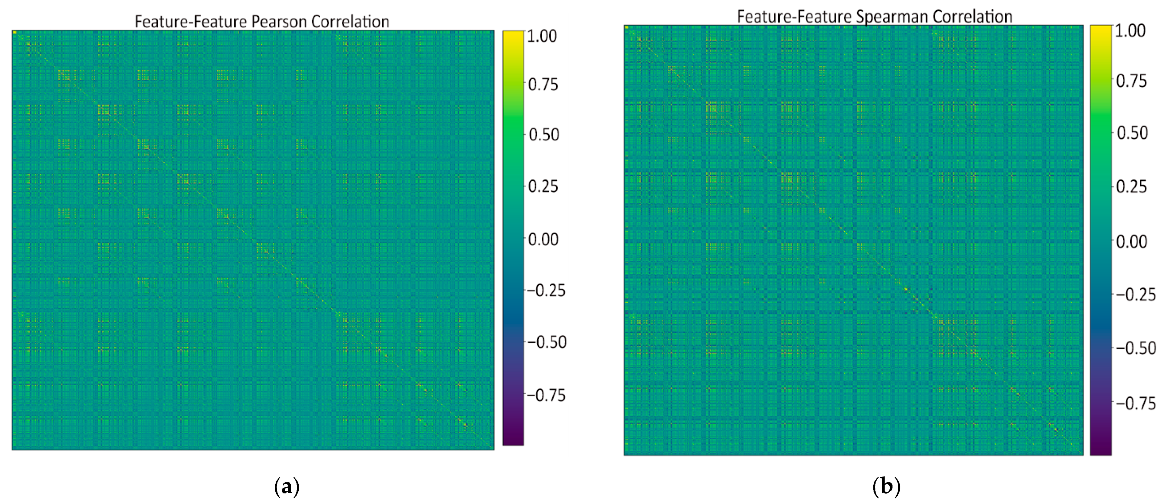
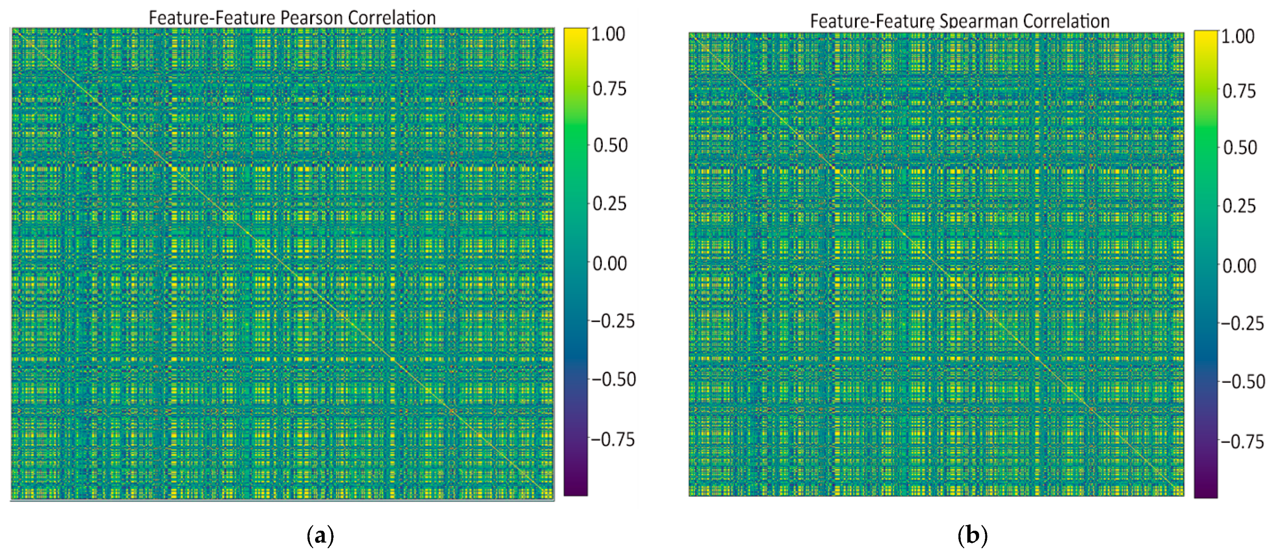
After the initial feature extraction process, which resulted in over 1000 extracted features, we carried out an exploratory data analysis (EDA) to understand which of those might truly drive PDAC vs. non-PDAC discrimination. We computed the feature—feature and feature—class correlation of Pearson and Spearman heatmaps and plots, respectively:

• Feature–feature Pearson heatmap (linear redundancy). A handful of bright off-diagonal blocks revealed groups of first-order and wavelet-based texture features that rise and fall almost in lock-step (|r| > 0.9), while the majority of pairs sat in the mild 0.2–0.5 range. These blocks signaled clear redundancy: it was safe to keep just one representative per block when we later pruned at ρ ≈ 0.9 without losing information.
• Feature–feature Spearman heatmap (monotonic redundancy). The Spearman map looked virtually identical to the Pearson one, confirming that the strong linear ties are also monotonic. Because no “new” high-ρ patterns appeared, a single Pearson-based threshold is enough to catch both linear and non-linear redundancies; no extra non-parametric filtering is needed.
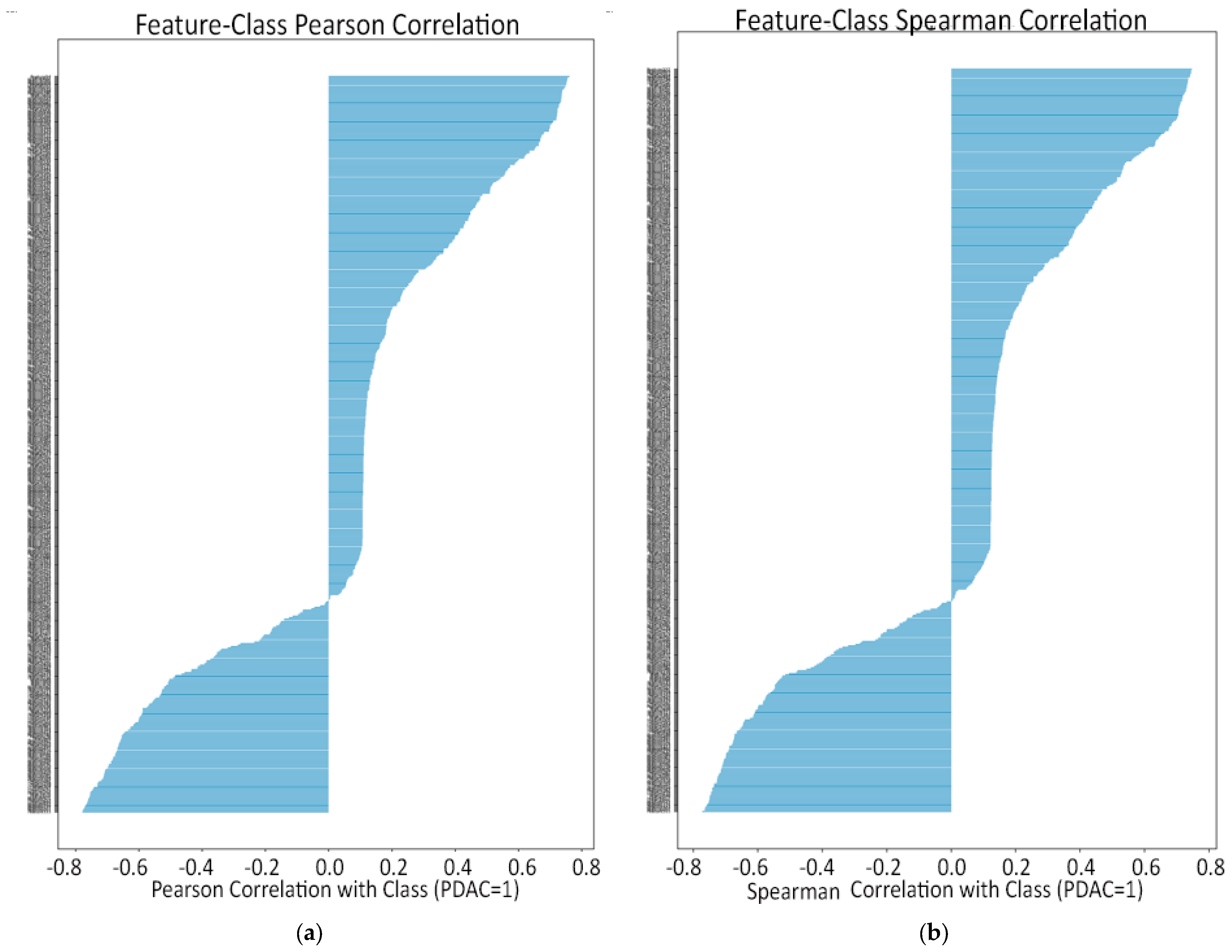
• Feature–class Pearson plot (linear predictive power). Only a small subset of radiomics reached r ≈ 0.6–0.8 with the PDAC label, while most hovered near zero. Those high-r features became prime candidates for univariate selection, but the plot also underlined the need for further pruning as two top-ranked features can still duplicate each other’s signal.
• Feature–class Spearman plot (monotonic predictive power). Ranking the data produced the same short list of standout predictors, indicating that their association with PDAC is robust, not just linear. No feature showed a high Spearman yet low Pearson, so non-linear monotonic effects are minimal; the same top features drive both metrics.

The feature–feature Pearson and Spearman heatmaps are illustrated in Figure 2, while the feature–class Pearson and Spearman plots are illustrated in Figure 3. These visualizations help guide interpretation but are not used for selection directly.

Moving forward to the feature selection pipeline, from more than 1000 extracted radiomic features, we constructed a two-stage feature-reduction strategy designed to yield a small, stable, and reproducible signature. First, we performed a structured hyper-parameter grid search to identify optimal filtering thresholds. On the Siemens/Philips training split, we evaluated combinations of four variance cut-offs (0, 10⁻⁴, 10⁻³, 10⁻²), three correlation caps (|r| = 0.90, 0.95, 0.99), and seven univariate keeper sizes (top-50 to top-1000 by f-ANOVA or mutual information). All configurations were assessed inside a 10-fold stratified cross-validation loop using three quick classifiers (L1-logistic, Random Forest, XGBoost). The triplet that most consistently maximized mean ROC-AUC was: variance > 10⁻⁴, keep the top-500 f-ANOVA features, and prune any pair with |r| > 0.90.

Then we applied an unsupervised filtering on the full training set by applying those thresholds removed obvious noise in three passes:

(a)

Low-variance cull—attributes that barely varied across patients were dropped.

(b)

Univariate ANOVA—the 500 radiomics with the strongest classwise F statistic were retained.

(c)

Correlation pruning—within that pool, for every pair whose Pearson |r| exceeded 0.90, the feature with the lower individual F ranking was discarded.

This left 137 medium-to-high-signal features that were largely decorrelated yet still spanned all image families (original, wavelet, LoG).

Then, further down the list, we embraced the idea that a good feature should be re-discoverable by different algorithms on repeated resampling of the data. Fifty bootstrap re-splits of the training set were run; on each resample, we fitted the following:

(1)

an L1-regularized logistic regression (linear, sparse),

(2)

a 200-tree Random Forest (non-linear, bagging), and

(3)

an XGBoost ensemble (non-linear, boosting).

For every model we recorded, which variables crossed that model’s own mean-importance threshold. Over the 50 runs, L1-logistic deemed 20 variables relevant at least once, Random Forest 31, and XGBoost 6.

Then, we applied a consensus and complementarity rule rather than simply taking the union. We applied the following:

• Features jointly selected by Random Forest ∩ XGBoost (17 features) were kept as robust non-linear predictors, and
• Features unique to LASSO but not present in the tree intersection (7 features) were added to preserve complementary linear effects.

This produced a 24-feature consensus panel that balanced linear and non-linear evidence while avoiding blatant overlap.

Lastly, a final qualitative check removed eight items that, despite passing the automated screen, were still highly inter-correlated with peers once the panel was viewed holistically or showed erratic behavior on the validation set. The surviving 16 features, spanning LoG first-order intensities, multi-scale GLSZM/GLRLM texture and wavelet-filtered GLCM statistics, constituted the input to every downstream machine-learning experiment.

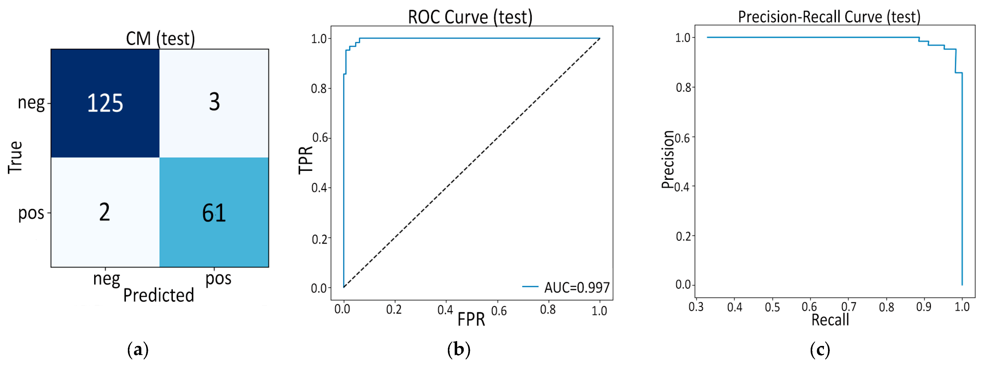
Moving to the data modeling part, for the classifier selection, on the held-out Siemens/Philips internal test split (191 cases), we bench marked four classical algorithms (k-Nearest Neighbors, L1-logistics, XGBoost, SVM EBF kernel), each fed with the same 16-feature radiomic signature and hyper-tuned only on the training folds. K-Nearest Neighbors fell short once sensitivity was weighed against calibration, while L1-logistic offered interpretability but missed several positives (sens ≈ 0.90). XGBoost posted the single highest AUC (0.999 ± 0.002) and near-perfect accuracy, yet its extreme confidence translated into the lowest Brier score and raised concerns of over-fitting to the modest sample size. The RBF-kernel Support Vector Machine provided the best balance of AUC = 0.997, accuracy = 0.974, sensitivity = 0.968, specificity = 0.977 and a reassuring Brier of 0.021, demonstrating both discrimination and well-behaved probability estimates without excessive complexity. We therefore selected the SVM as our radiomics champion and froze its weights.

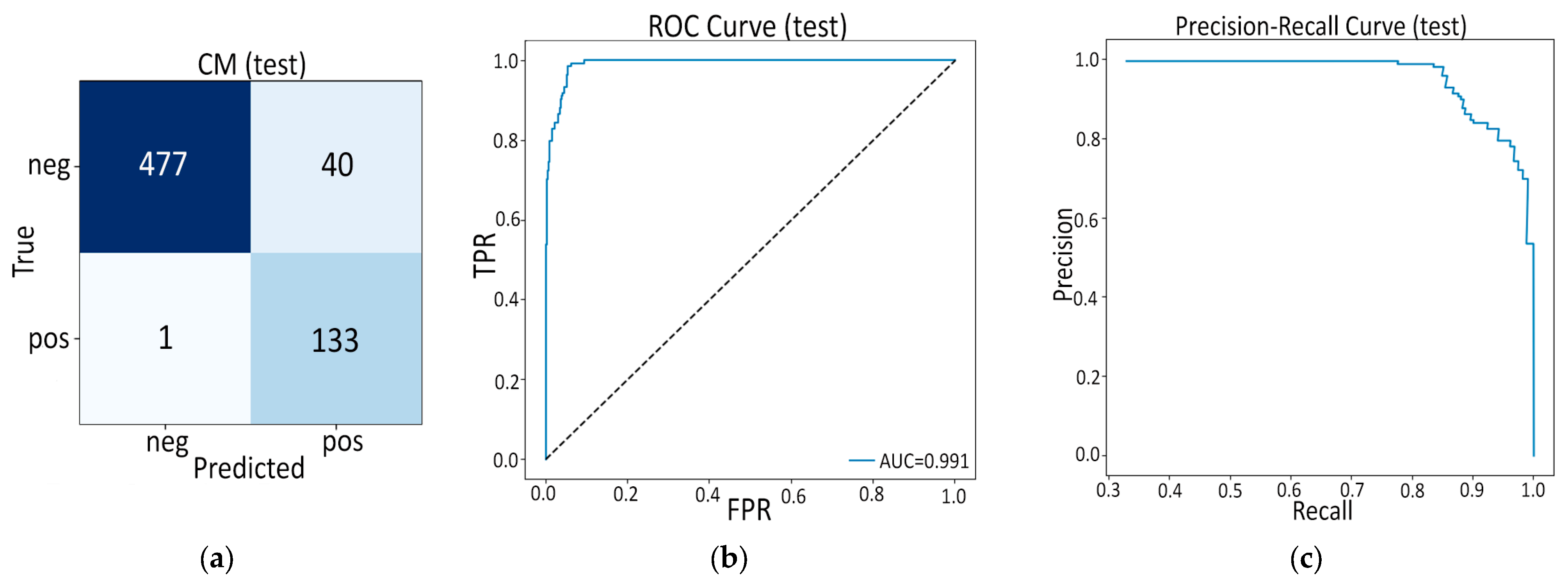
Crucially, no additional re-training or threshold tweaking was performed before deployment to the Toshiba external cohort (651 cases). Using the identical 16-feature scaler, the SVM generalized with an accuracy of 0.937, a near-perfect sensitivity of 0.993 and an AUC of 0.991, only a modest drop in specificity (0.923) compared with internal testing and an acceptable Brier of 0.053. These stable out-of-vendor results confirmed that the low-dimensional, carefully filtered radiomic vector and the SVM decision boundary learned solely on Siemens/Philips data retained predictive power when confronted with a completely unseen scanner domain, justifying its role as Model A and as the radiomics branch in both fusion variants.

The results of internal and external evaluation are summarized in

Table 2. Results of Model A for internal and external tests.

Metric	Internal Test (Siemens + Philips, n = 191)	External Test (Toshiba, n = 651)
Accuracy	0.974	0.937
Sensitivity (Recall PDAC)	0.968	0.993
Specificity	0.977	0.923
Precision (PPV)	0.953	0.769
F1-score	0.961	0.866
ROC-AUC	0.997	0.991
Brier score	0.021	0.053

. The confusion matrices, ROC curve and Precision—Recall curves for both internal and external evaluation are illustrated in Figure 4 and Figure 5, respectively.

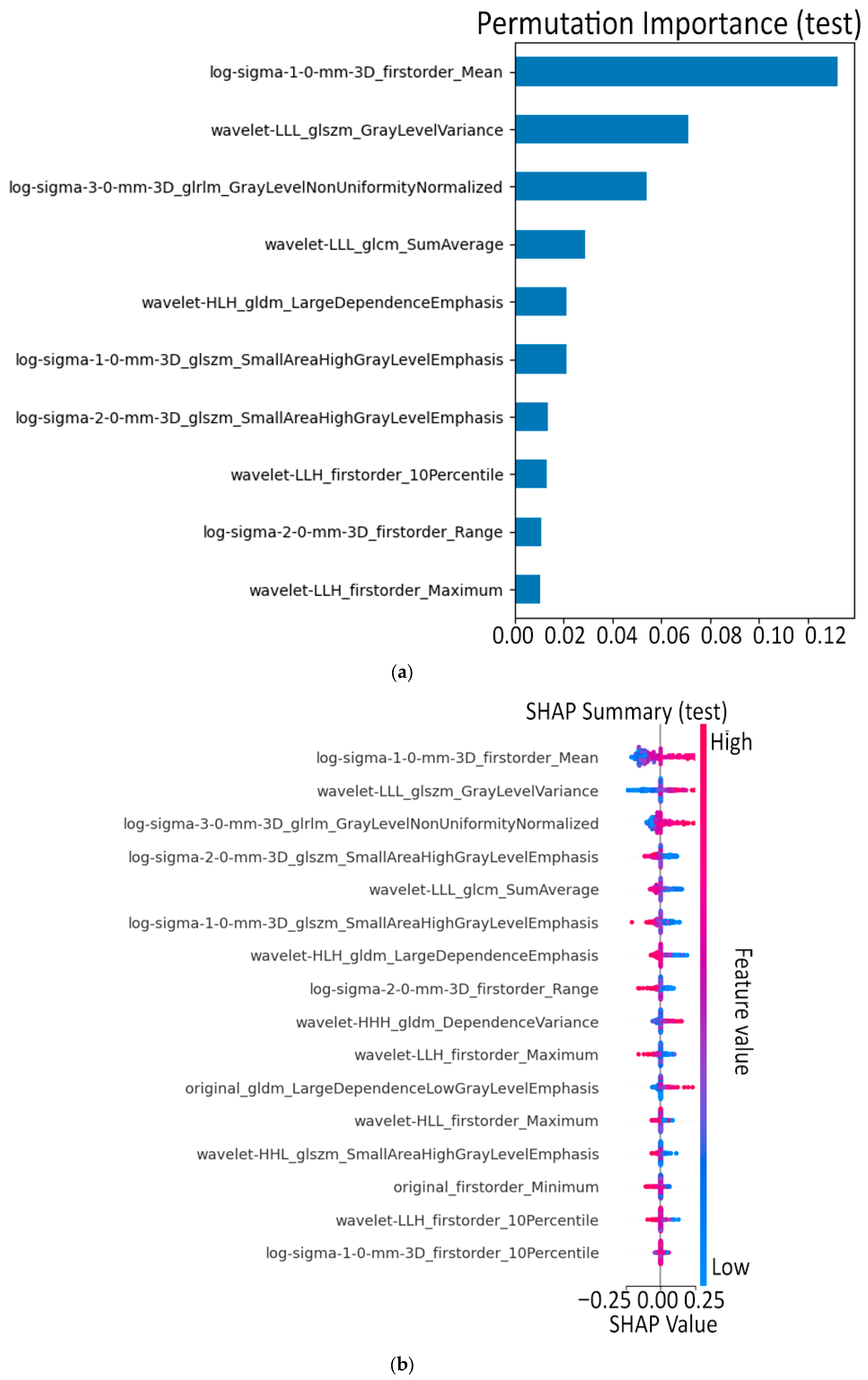
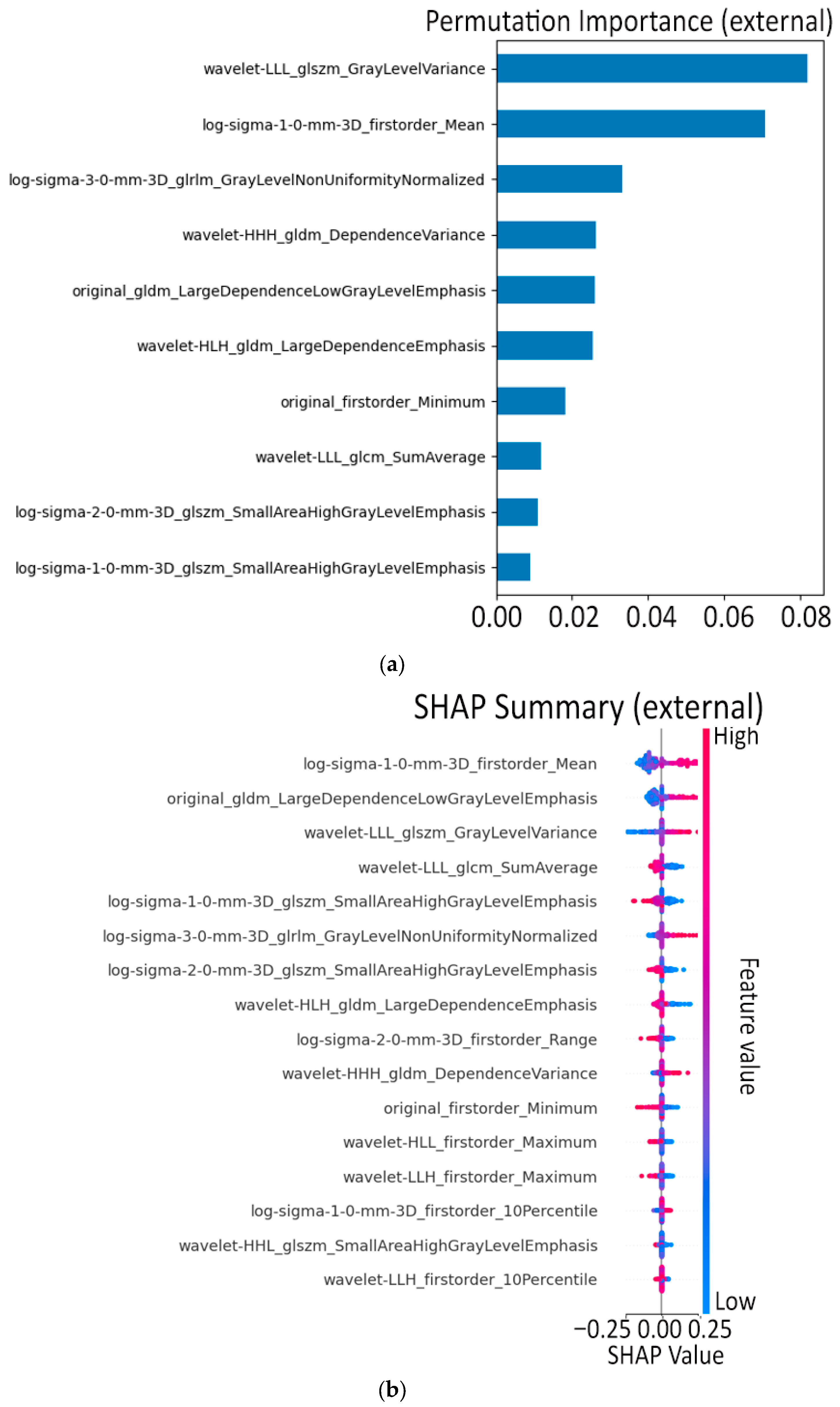
On the internal and external test sets, we quantified feature influence with two complementary tools, permutation importance [19], and SHapley Additive exPlanations (SHAP) summary plots [20].

Permutation-importance is a global ablation test: we shuffle one feature at a time, re-score the model, and plot the ten whose shuffling hurts AUC the most. Showing only the top ten keeps the bar chart legible, but it means less-critical variables are hidden. SHAP, by contrast, visualizes every feature and every patient. Each dot’s horizontal position shows how much that feature pushed the logit up or down for one case, and the overall “width” of the cloud indicates global influence. That is why all 16 radiomic inputs appear in the SHAP beeswarm while only the ten most disruptive appear in the permutation plot.

Across both internal and external cohorts, the same texture-heterogeneity markers dominate. Internally, the strongest drivers are log-sigma-1-0-mm³ first-order Mean (fine-scale intensity average), wavelet-LLL GLSZM GrayLevelVariance (coarse-scale gray-level scatter) and log-sigma-3-0-mm³ GLRLM GrayLevelNonUniformityNormalized. These three account for the largest AUC drops when permuted and have the widest SHAP spreads. Externally, the ordering shuffles slightly—wavelet-LLL GLSZM GrayLevelVariance edges into the top spot—but the same trio plus original GLDM LargeDependenceLowGrayLevelEmphasis remain the most informative, confirming that fine- and coarse-scale texture irregularity is the key radiomic signature the SVM relies on in unseen Toshiba data.

Permutation importance and SHAP summary plots for both internal and external tests are illustrated in Figure 6 and Figure 7, respectively. The entire pipeline of the proposed methodology, referring to Model A, is illustrated in Figure 8. Figure 8 contains multiple sub-blocks, all stages execute sequentially with fixed hand-offs between them. In practice, PyRadiomics extraction is the only computationally heavy step, while the multi-pass feature-selection pipeline is lightweight and presents no bottleneck since each successive filter operates on a progressively smaller subset of features. More analytically, the coordination and computational behavior of the full pipeline is as follows:

• Pipeline coordination and execution order. All stages in Figure 8 operate in a strictly sequential manner. The workflow therefore executes as follows: image harmonization, feature extraction, feature selection, model benchmarking and internal testing of four models, internal and external testing.
• Computational load. The most computationally expensive stage is the initial PyRadiomics feature extraction, which generates >1000 descriptors per case from original, wavelet, and LoG volumes. This step is GPU-free and parallel, allowing multi-core execution with near-linear speedup. In contrast, the downstream feature selection and pruning operations (variance filtering, univariate ANOVA, and correlation-based pruning) are lightweight.
• No bottleneck in the feature-selection pipeline. Although Figure 8 shows multiple sub-blocks, each operates on a progressively smaller subset of features and therefore executes very quickly. The only resampling and heavy part is the 50-bootstrap model-based stability test which uses simple linear/logistic models and shallow tree ensembles, requiring only minutes on a standard workstation.
• Coordination between blocks. Each block passes a fixed-size output table (CSV/NumPy array) to the next stage. No stage depends on dynamic control flow. The pipeline is therefore robust, modular, and easy to reproduce and as a result, the exact implementation will publicly be released to ensure full transparency.

3.2. Model B: Pure Deep Learning

Our second approach makes use of a 3D convolutional network to learn directly from the CT volumes. Our methodology works simultaneously in a two-way approach. We train, validate and evaluate the model with our internal and external subsets, but simultaneously we extract 512 features for each subset (train, validation, internal and external test) in order to perform a feature selection later with the aim of using the best extracted features in the fusion model.

Once all scans and their corresponding pancreas masks had been oriented, resampled, intensity-normalized, and clipped to soft-tissue ranges, we used the mask to compute a tight three-dimensional bounding box around the pancreas. This ensured that every example entering the network would focus on the organ of interest and avoid wasted computation on surrounding air or unrelated anatomy. In practice, we found that a fixed output size of 224 × 160 × 160 voxels reliably captured the pancreas across patients once the box was centered and symmetrically padded or cropped as needed.

With volumes cropped, we defined a light yet expressive augmentation scheme during training, small random left–right flips, tiny rotations and scale jitter, and minute added noise in order to encourage the model to generalize across scanner differences and patient positioning. No augmentation was applied at evaluation time. We also re-weighted each case’s contribution to the loss based on whether its mask was manual or automatically generated, giving slightly more importance to the manually segmented ground truths.

Our core network is a three-dimensional ResNet-18 backbone whose first convolution was adapted to accept a single-channel CT input. After the final residual block, we inserted a two-stage attention module: first, a channel-wise attention that learns which feature maps matter most, then a spatial attention that sharpens focus to the most informative voxels. Together, these “CBAM” blocks help the network ignore irrelevant background and concentrate on subtle textural or morphological cues within the pancreas. After settling on our CBAM-augmented 3-D ResNet-18 architecture and loss-weighting scheme, we divided our Siemens/Philips cohort into disjoint training (≈880 scans), validation (≈190 scans), and internal test (≈166 scans) splits. Our ultimate goal is to choose hyperparameters entirely on the validation set and then report final performance on the held-out internal test and an external Toshiba cohort.

Training proceeded under a standard cross-entropy objective weighted to offset the PDAC/non-PDAC imbalance, with an initial learning rate of 1 × 10⁻⁴ that gradually decayed over eighty epochs and early stopping was triggered if the validation AUC failed to improve for fifteen straight epochs. We also applied a short warmup of five epochs at a lower learning rate to stabilize the very first steps. Batch size was limited by GPU memory to four volumes at a time, and gradient accumulation was used to mimic a slightly larger effective batch when helpful.

Once convergence was reached, we froze the network and removed its final two-class output layer, using the 512-dimensional vector just after the global-pooling and normalization steps as a descriptive “deep embedding” of each pancreas.

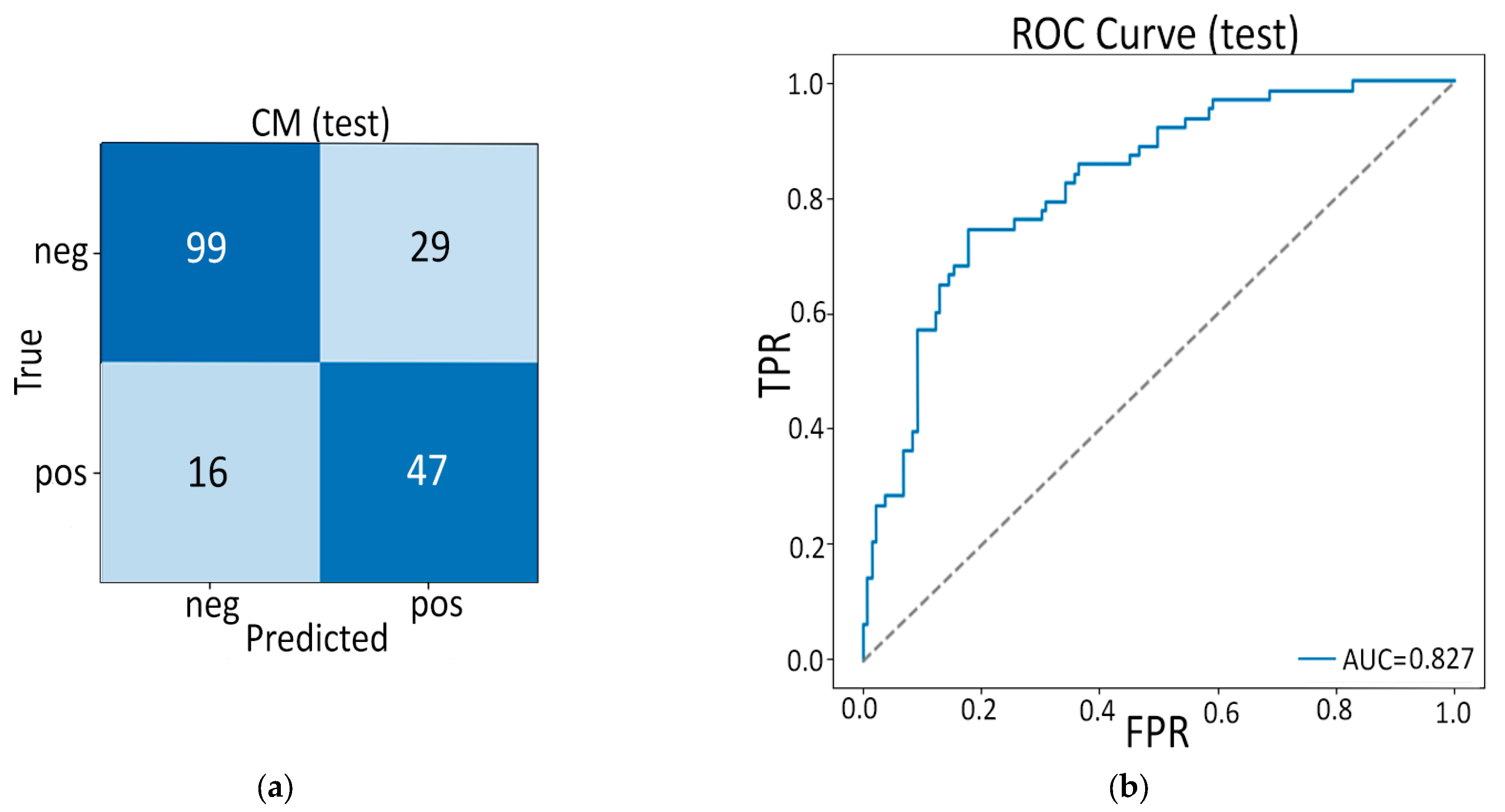
After completing training and selecting the checkpoint with the highest validation ROC–AUC, we evaluated the model once on the internal test set of Siemens/Philips scans that was never used during training or hyper parameter tuning. These ≈ 166 volumes underwent the same preprocessing pipeline, center-crop or pad to (224 × 160 × 160) voxels, Z-normalization and were passed through the 3-D CBAM ResNet-18 to produce PDAC versus non-PDAC logits.

For each case, we applied the probability threshold determined on the validation split to convert softmax outputs into binary predictions. We then computed the ROC–AUC to measure discrimination, overall accuracy, sensitivity (PDAC recall) and specificity (non-PDAC recall), and the F1-score to balance precision and recall under class imbalance. A full classification report (precision, recall, F1 for each class, plus support) and a confusion--matrix heat map were generated to visualize true versus predicted labels. In parallel, we extracted the 512-dimensional deep embedding for each test volume by tapping the network’s penultimate layer.

For external validation, we held out 70% of the Toshiba cases as a truly unseen test set after reserving 30% for calibration. The calibration step used the best checkpoint from our Siemens/Philips training to adjust the decision threshold for the Toshiba domain. We loaded each calibration volume, applied the same center-crop/pad and intensity normalization transforms, and passed them through the network to collect a PDAC probability for every case. By sweeping possible thresholds and computing the Youden index (sensitivity—1 − specificity), we identified the cutoff that maximized balanced sensitivity and specificity on the calibration split. This new Toshiba-specific threshold was saved for subsequent testing.

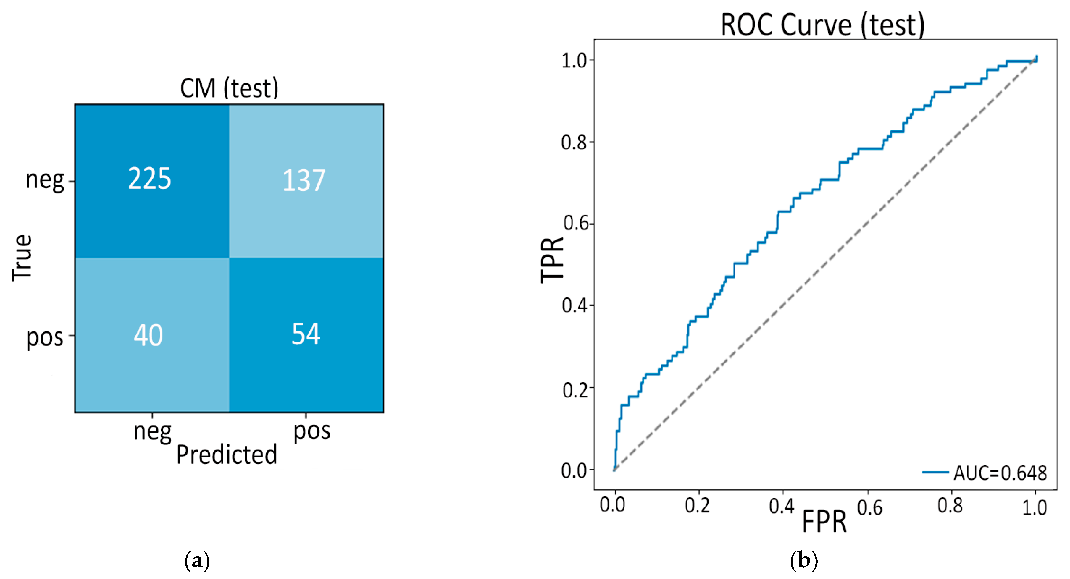
With the threshold fixed, we then evaluated the model on the remaining 70% of Toshiba scans. Each held-out volume underwent identical preprocessing and inference; volumes were classified as PDAC or non-PDAC by comparing the network’s predicted probability against the calibrated cutoff. From these classifications we computed the ROC–AUC to quantify discriminative power, overall accuracy, sensitivity (PDAC recall), specificity (non–PDAC recall), and F1-score to balance precision and recall under our class imbalance. We also generated a reliability diagram—plotting predicted probability bins against observed outcome frequencies, to check that our calibrated probabilities remained well-calibrated in this new setting, and we computed the Brier score as a holistic measure of probabilistic accuracy. All the results of the internal and external tests are included in

Table 3. Results of Model B for internal and external tests.

Metric	Internal Test (n = 191)	External Test (n = 456)
ROC-AUC	0.8268 (thr ≈ 0.2913)	0.6485 (thr ≈ 0.1416)
Threshold	0.2913	0.1416
Accuracy	0.7644	0.6118
Sensitivity (PDAC recall)	0.7460	0.5745
Specificity (non-PDAC recall)	0.7734	0.6215
Macro-avg Precision	0.7396	0.5659
Macro-avg Recall	0.7597	0.5980
Macro-avg F1-score	0.7455	0.5483
Weighted-avg Precision	0.7809	0.7323
Weighted-avg Recall	0.7644	0.6118
Weighted-avg F1-score	0.7691	0.6479
non-PDAC Precision/Recall/F1	0.8609/0.7734/0.8148	0.8491/0.6215/0.7177
PDAC Precision/Recall/F1	0.6184/0.7460/0.6763	0.2827/0.5745/0.3789

.

The confusion matrices and ROC curves for the internal and external evaluation are illustrated in Figure 9 and Figure 10, respectively.

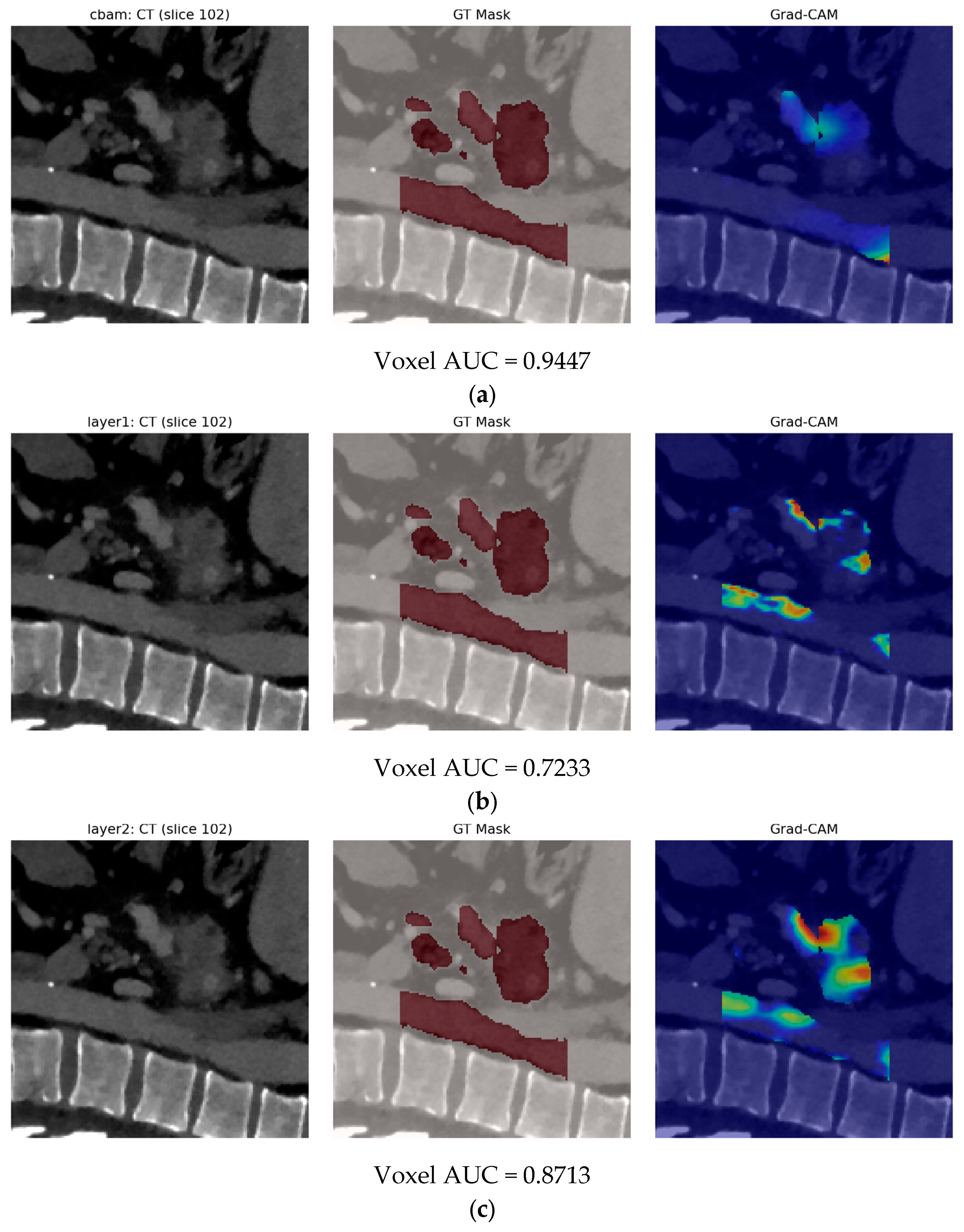
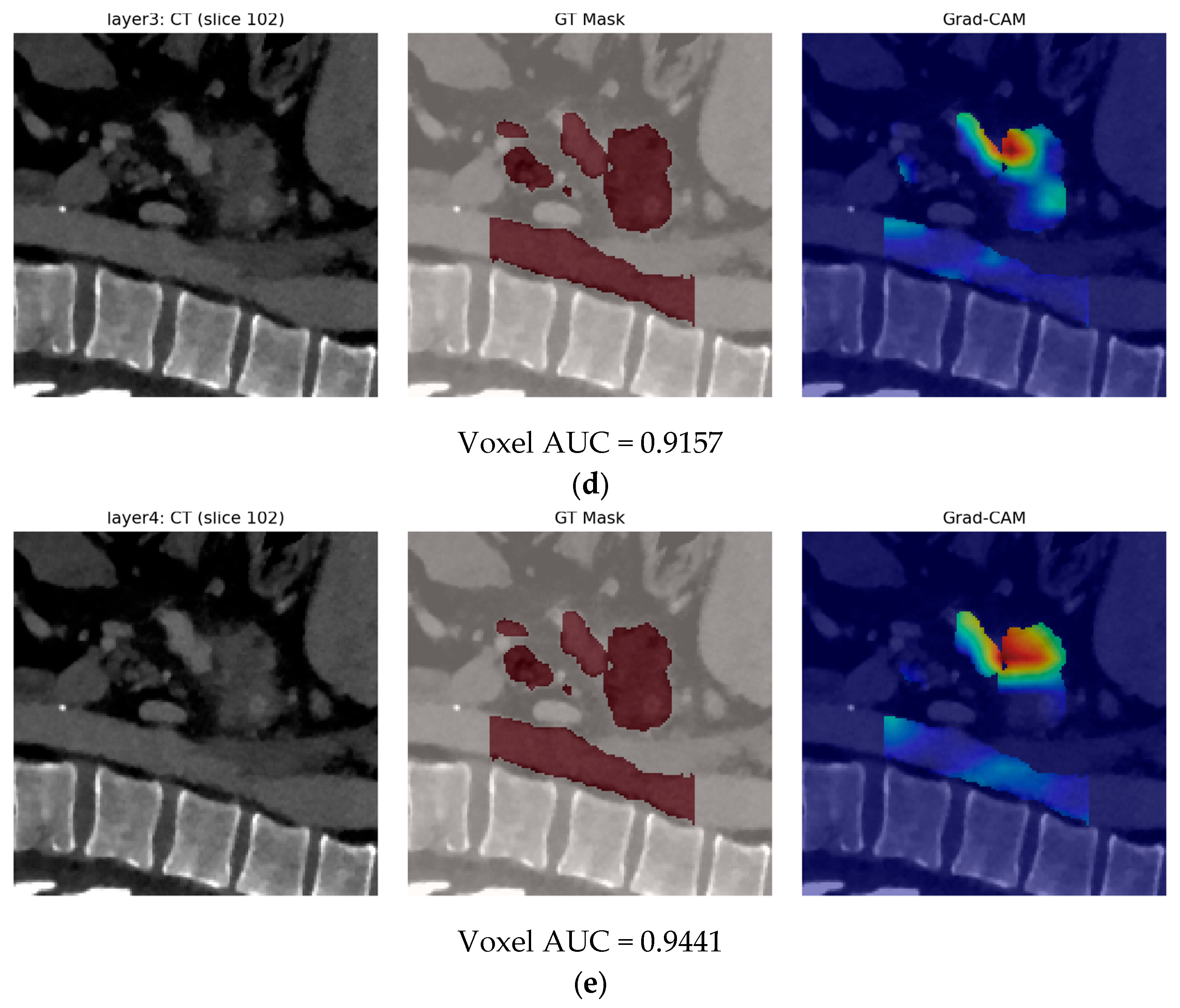
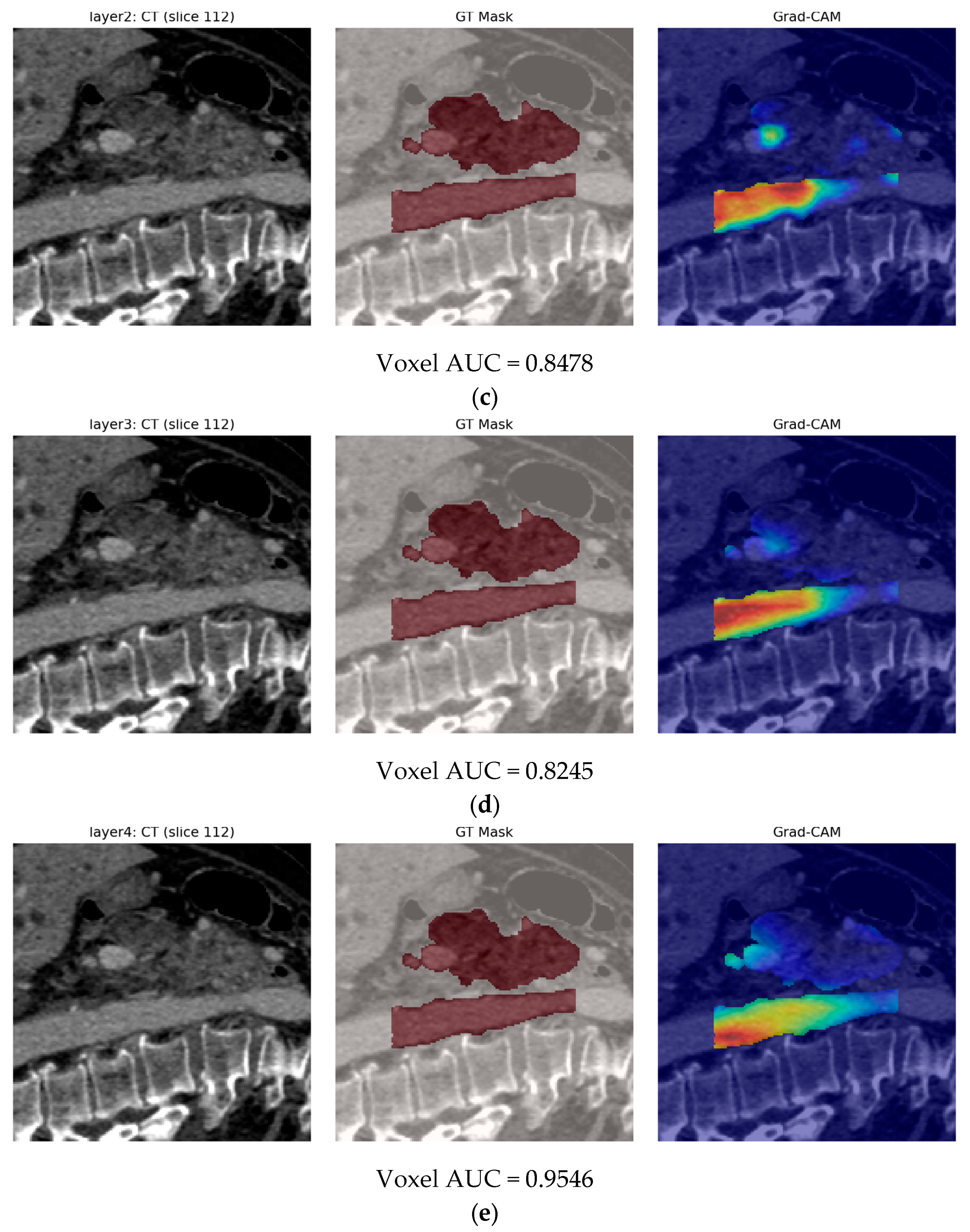
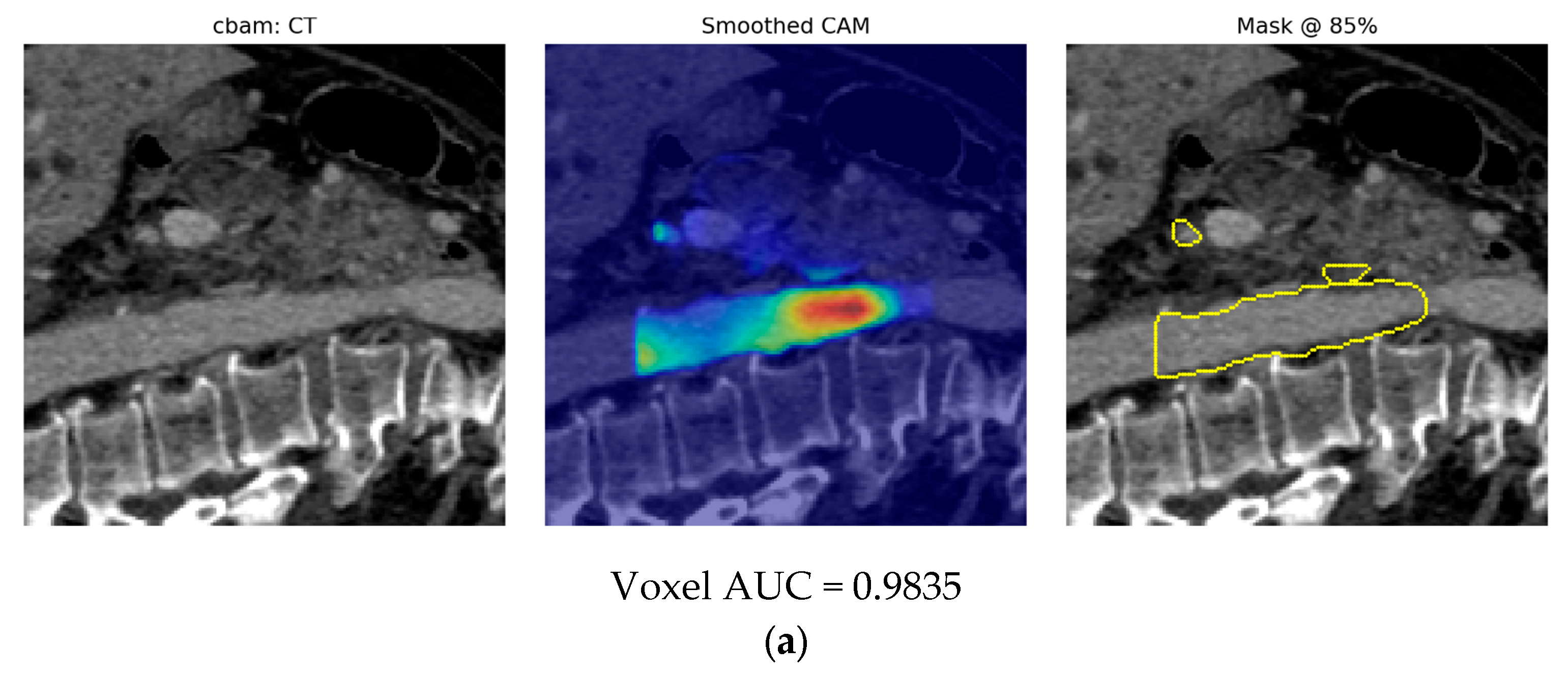
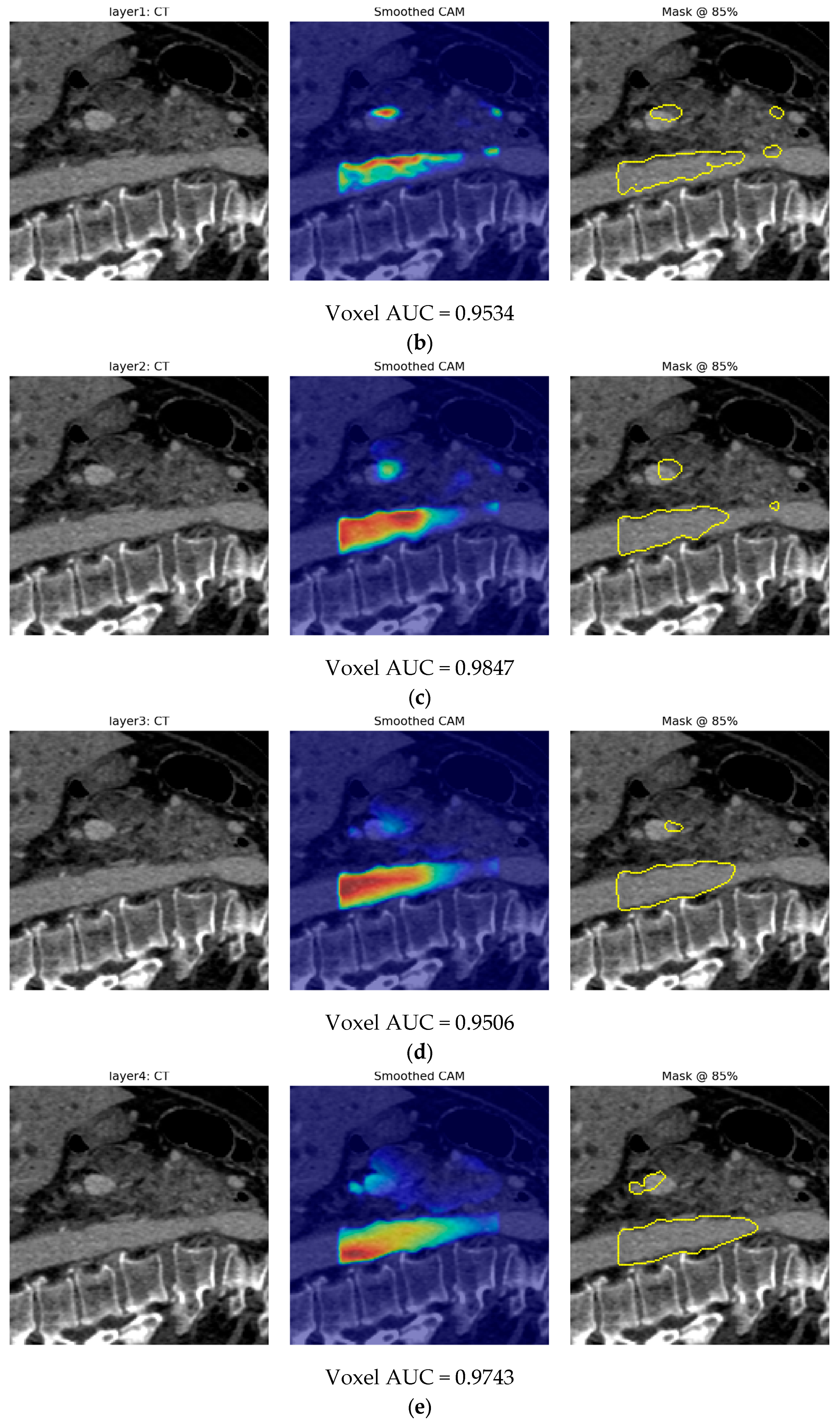
To build trust in our purely deep model (Model B) and to guide its later fusion with radiomics, we applied rich, volumetric Grad-CAM [21] analyses to every major convolutional block. Starting from the final, best-checkpoint 3-D CBAM-ResNet-18, we fed each held-out CT volume (after the same center-crop/pad and Z-normalization used at inference) forward through the network and then back-propagated from the PDAC logit into the feature maps of layers 1, 2, 3, 4 and the CBAM module. At each layer, we globally pooled the gradients to produce per-channel weights, multiplied those against the corresponding 3-D activation maps, applied ReLU, and trilinearly up-sampled back to the original (224 × 160 × 160) resolution, resulting in a coarse, 3-D “heat volume” that highlights which voxels most drove the PDAC decision at that depth.

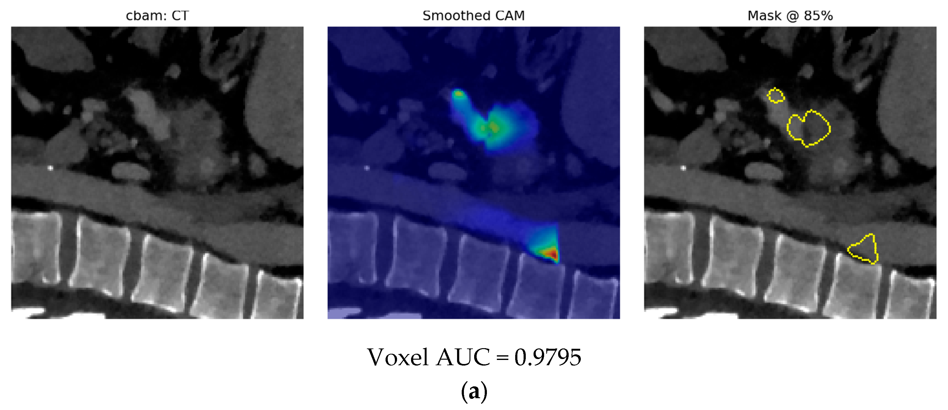
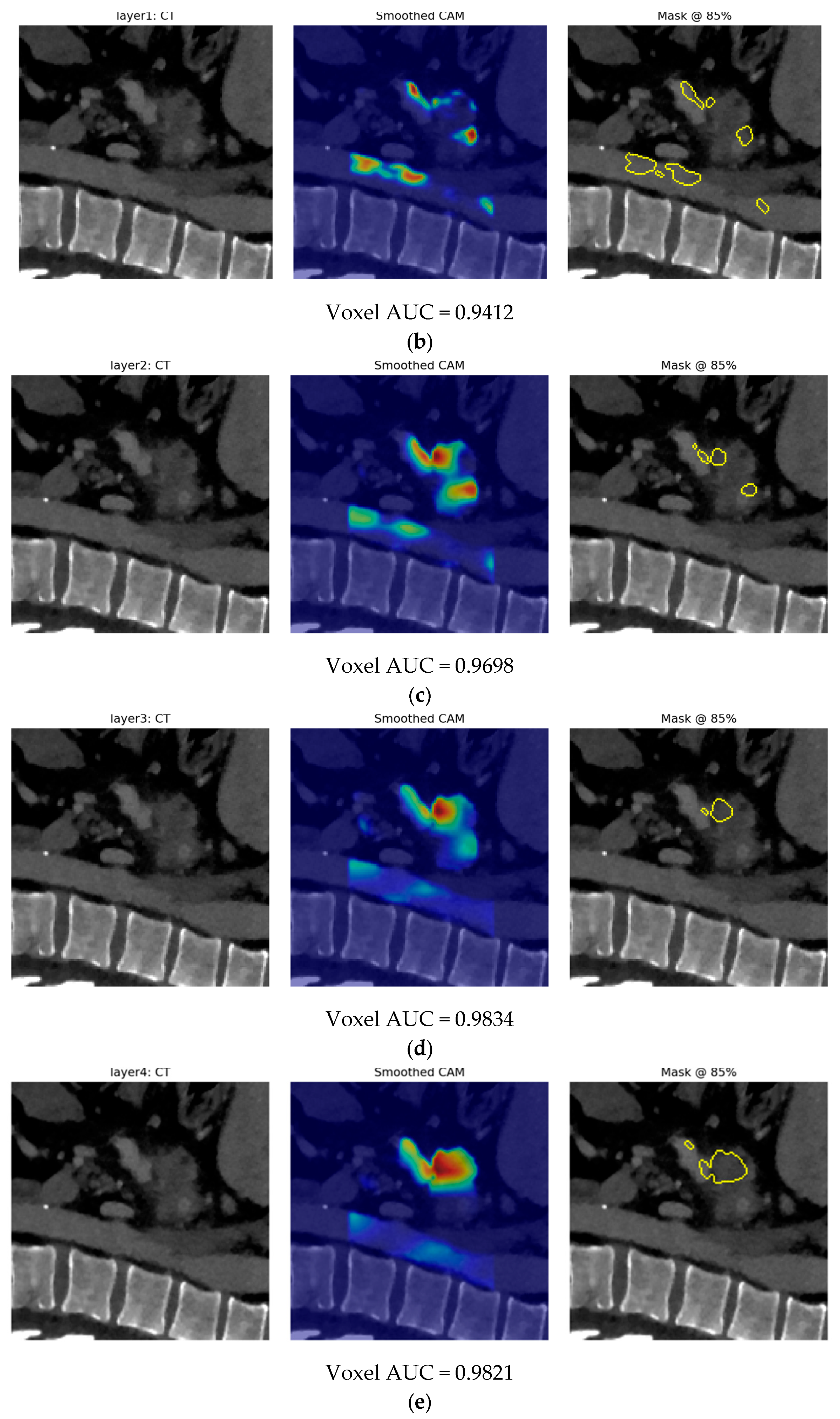
We visualized these heat volumes in two complementary ways. First, for each layer we found the centroid slice of the radiologist’s tumor mask (mean Z-index of mask voxels) and overlaid the continuous CAM on the raw CT slice beside the ground-truth mask, producing intuitive 1 × 3 panels (CT∣Mask∣Grad-CAM). Second, we smoothed each 3-D CAM with a small Gaussian (σ = 1 voxel) and swept percentile thresholds around a nominal 85% value to binarize the map by choosing the threshold that maximized the 3-D Dice overlap with the true mask, we quantified both the best attainable segmentation accuracy and the centroid error (distance between CAM vs. mask centroids) per layer.

For the internal dataset, across layers, voxel-wise AUC (treating CAM intensity as a continuous predictor of being “inside tumor”) rose markedly, from ~0.72 at layer 1 to ~0.94–0.98 at layer 4 and in the CBAM module, demonstrating that deeper features become more tumor-focused. The optimal 3-D Dice similarly peaked around 0.90 at layer 4, with centroid localization errors shrinking from ~9 voxels (layer 1) down to ~2 voxels (layer 4). Qualitatively, the hottest CAM regions align tightly with the pancreatic head/body and peri-pancreatic lesion, rather than drifting into irrelevant structures like vertebrae or vessels.

These Grad-CAM results confirm two crucial points: first, our network indeed “looks” at the right anatomy when deciding PDAC, lending clinical face validity; and second, its final deep features encapsulate a strong, spatially coherent tumor signature, precisely the kind of focused, high-level information that fusion with handcrafted radiomics can amplify. By pinpointing both where and at which depth the model attends, this XAI (eXplainable Artificial Intelligence) analysis not only builds user trust but also informs the design of our downstream fusion head, ensuring we combine complementary insights from image-based and feature-based representations.

Indicative Grad-CAM representations across the CBAM layer and layers 1, 2, 3, 4 by following both approaches (using centroid slice and centroid percentile thresholds) for the internal test dataset are illustrated in Figure 11 and Figure 12, respectively. Figures include the corresponding voxel-wise AUC value to summarize the quantitative localization accuracy of each layer’s Grad-CAM map, to better clarify the difference in results obtained in each layer.

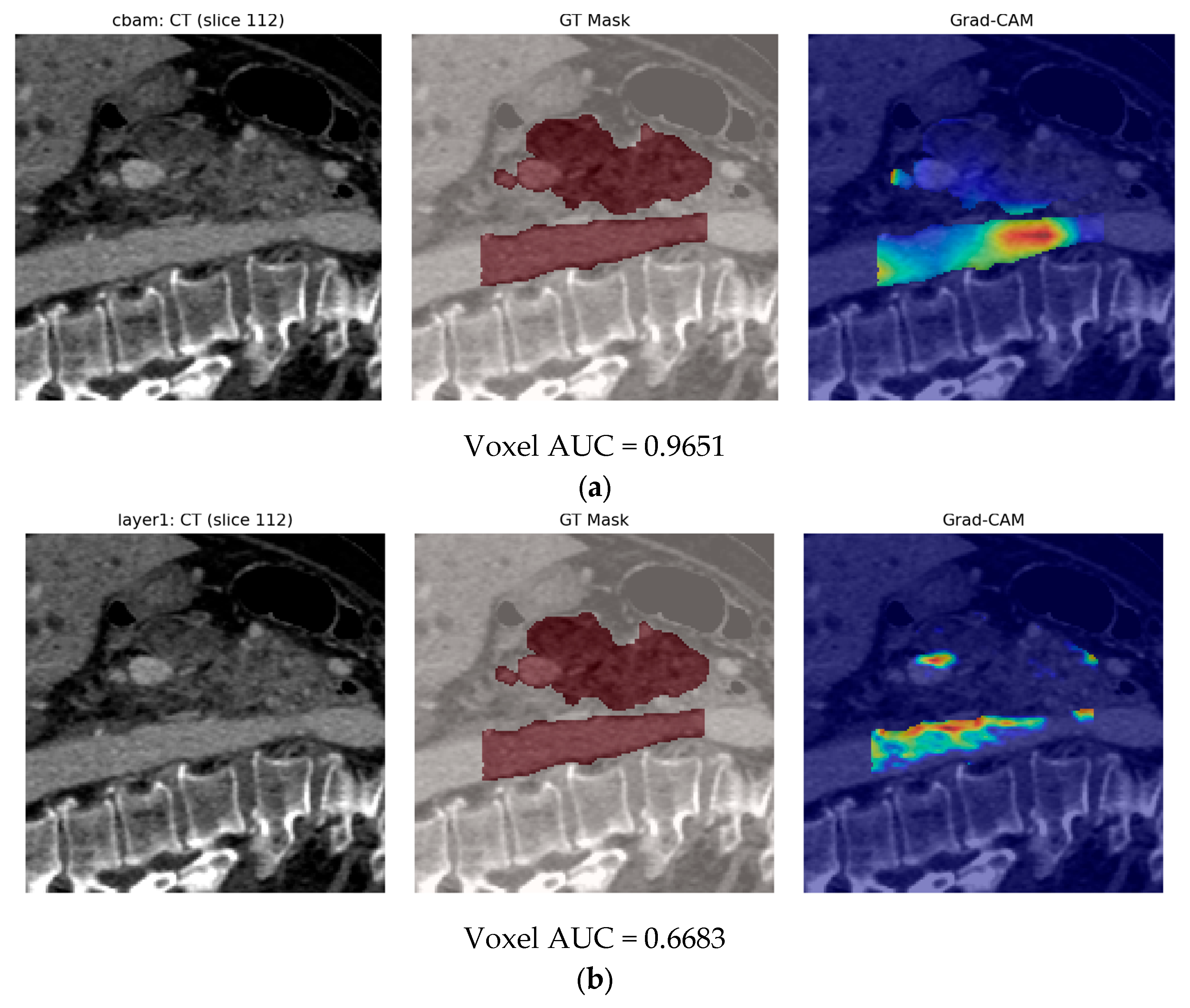
For the independent Toshiba cohort, the Grad-CAM analysis paints a subtler picture than on the internal data. Voxel-wise AUC rises from roughly 0.67 in the very first residual block to 0.95 in block 4 and 0.97 inside the final CBAM attention module. In other words, while the earliest filters already achieve fair localization, they remain distracted by non-neoplastic parenchyma and peri-pancreatic fat, only converging onto the true tumor–duct complex once the representation has passed through three to four convolutional stages and the dedicated attention gate. Dice curves tell the same story: at an 85% CAM-intensity threshold, the best overlap plateaus at ≈0.26, and centroid errors expand from ≈8 voxels in layer 1 to ≈21 voxels in layer 4. Qualitatively, the deepest heatmaps still illuminate the pancreatic body/tail lesion correctly, but shallower layers sprinkle low-grade activations over adjacent gastric wall and mesenteric fat, an expected domain-shift artifact, because Toshiba scans were acquired with a different reconstruction kernel and generally exhibit smoother noise textures. These observations justify the small, but noticeable drop in early layer localization performance (e.g., voxel-AUC 0.78 in layer 2 versus > 0.9 internally). Thus, even under cross-vendor conditions, our attention pipeline remains anatomically meaningful at depth.

Grad-CAM representations across the CBAM layer and layers 1, 2, 3, 4 by following both approaches (using centroid slice and centroid percentile thresholds) for the external Toshiba test dataset are illustrated in Figure 13 and Figure 14, respectively. Figures include the corresponding voxel-wise AUC value to summarize the quantitative localization accuracy of each layer’s Grad-CAM map, to better clarify the difference in results obtained in each layer.

After finishing the training and evaluation part, we shifted our focus back to the feature extraction and selection process. After the initial feature extraction process, which resulted in 512 extracted features (deep embeddings), we carried out an exploratory data analysis (EDA) in order to understand which of those features might truly help discriminate between PDAC vs. non-PDAC. We computed the feature—feature and feature—class correlation of Pearson and Spearman heatmaps and plots, respectively:

• Feature–Feature Pearson Correlation. The 512 × 512 Pearson heatmap shows clear, bright blocks along the diagonal—each block (20–60 channels) with r > 0.9 indicates groups of nearly identical deep features. Outside these blocks, correlations drop to 0.3–0.7, and negative correlations are virtually absent. This confirms heavy redundancy and justifies collapsing each block before selection.
• Feature–Feature Spearman Correlation. The Spearman map nearly mirrors the Pearson blocks, showing that those same channel groups also rank-order together, not just vary linearly. A few moderate inter-block ties soften slightly, but no new inverse relationships appear. In short, rank-based redundancy aligns with raw-value redundancy.
• Feature–Class Pearson Correlation. Ranking channels by Pearson r reveals only a handful with |r| > 0.5 that strongly rise in PDAC or non-PDAC, while most features lie between −0.2 and +0.2. The extreme positive bars pinpoint tumor-sensitive probes; the extreme negative bars flag healthy-tissue detectors. These top correlates guide our univariate filtering.
• Feature–Class Spearman Correlation. The Spearman ranking yields almost the same small set of top channels (ρ ≈ ±0.7–0.8) but shows a sharper drop-off beyond the strongest monotonic features. This tighter “elbow” confirms that only a few embeddings reliably order PDAC above non-PDAC. Those top monotonic channels form a conservative shortlist for selection.

The feature–feature Pearson and Spearman heatmaps, and the feature–class Pearson and Spearman plots are illustrated in Figure 15 and Figure 16, respectively. Same as previously, these visualizations are presented towards helping guide interpretation but are not used for selection directly.

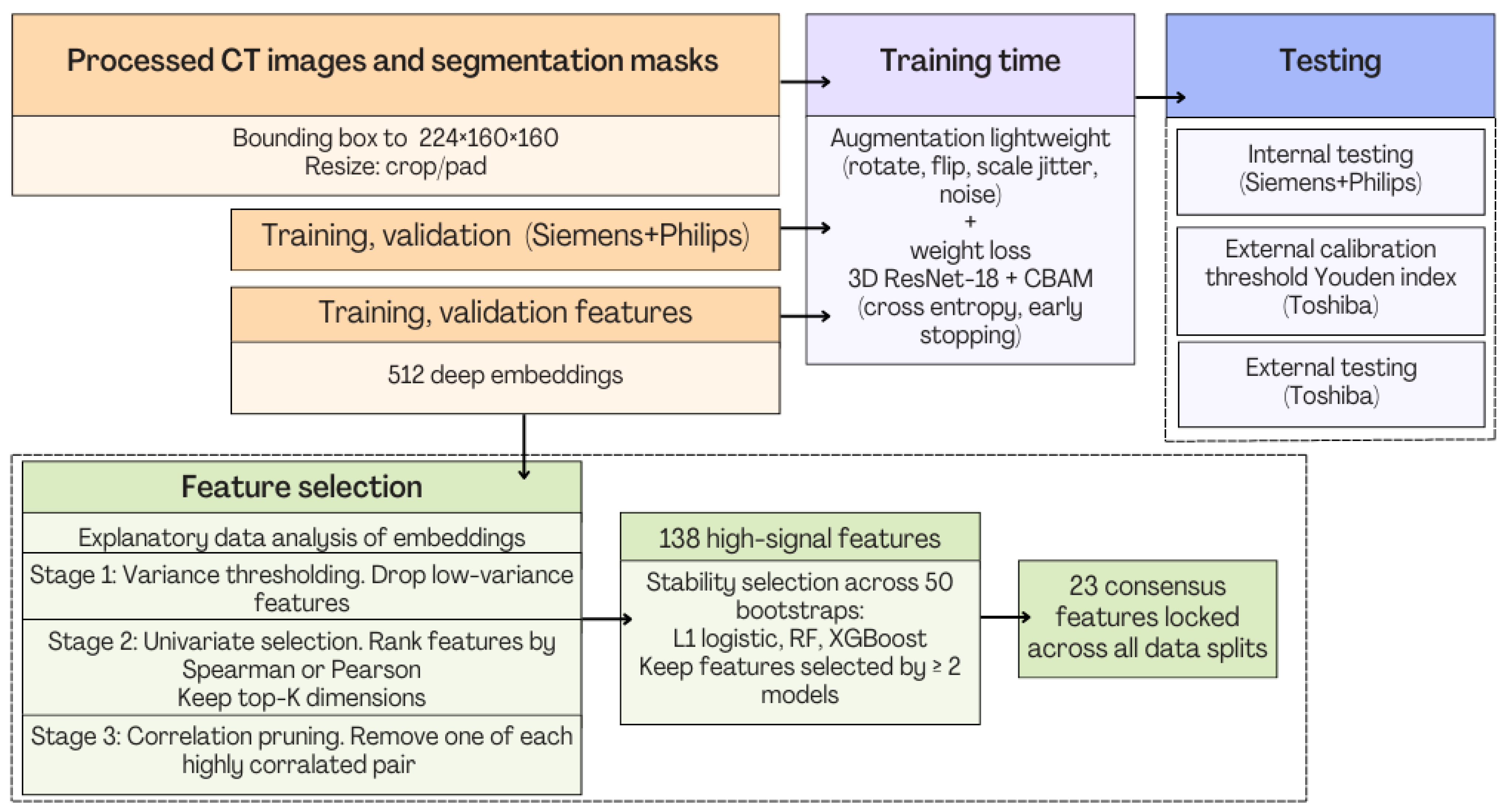
Next, we applied a three-stage filtering pipeline to whittle down our 512-dimensional embeddings to a lean set of 138 high-signal features. First, we used variance thresholding, sweeping thresholds from 0 through 1 × 10², to eliminate “dead” channels whose values barely varied across hundreds of Siemens/Philips scans. Those near-constant dimensions cannot help discrimination, so dropping them sharply reduced noise up front. Next, on the surviving features we ran univariate selection via SelectKBest: we ranked each dimension by its absolute Pearson r, mutual-information score, or Spearman ρ with the binary PDAC label, and kept only the top-K (where K varied from 50 up to the full 512). This ensured that every retained feature had demonstrated at least some individual association with disease status. Finally, we performed correlation pruning: for any pair of features whose absolute Pearson correlation exceeded our chosen cutoff (we experimented with 0.90, 0.95, and 0.99), we dropped one, guaranteeing that the remaining features carried non-overlapping information. Under our optimal settings (variance ≥ 1 × 10², mutual-information top-300, corr-thr = 0.90), this pipeline gave us 138 robust deep-feature dimensions to move forward with.

With that reduced pool of 138 candidates in hand, we turned to model-based stability selection to isolate the most reproducible signals. Over 50 bootstrap resamples of the training set, we fit three distinct “stability” models on each draw: an L1-penalized logistic regression (selecting based on nonzero coefficients), a random forest classifier (keeping features above mean Gini importance), and an XGBoost model (retaining features above mean gain importance). For every feature, we tallied how often it survived across all resamples and methods, then defined our final consensus set as those dimensions selected by at least two of the three models. This rigorous cross-model, cross-bootstrap approach distilled our pool from 138 down to 23 deep-embedding features, combining the linear discriminative power of L1 logistic with the non-linear insights of tree-based learners. Finally, we locked in those 23 consensus features across every dataset split, training, validation, Siemens/Philips internal test, and Toshiba external test. The proposed pipeline of the Model B methodology is illustrated in Figure 17.

In Figure 17, the feature-selection stage beneath the 512 deep embeddings was intentionally added to ensure that Model B could serve as a feature-generating branch for the fusion model (Model C), not only as a standalone classifier. Although the 3-D CNN produces 512 channels after global pooling, our exploratory analysis showed that these embeddings contain substantial redundancy (large r > 0.9 blocks) and only a small subset exhibits strong association with PDAC. Using all 512 deep embeddings as fusion inputs would increase noise, weaken interpretability and inflate the dimensional imbalance with respect to radiomics.

Therefore, we introduced a light three-stage filtering pipeline (variance thresholding, univariate selection, correlation pruning), followed by bootstrap stability-selection, to identify the most reproducible and non-redundant deep features. This design gave us a compact, stable set of 23 deep embeddings.

3.3. Model C

3.3.1. Model C1: Two-Stage Frozen Fusion

In our first fusion approach, we took the sixteen handcrafted radiomics features and the twenty-three deep CNN embeddings and simply stitched them end-to-end into a single 39-dimensional vector. By preserving the radiomics stream as an identity mapping and the deep stream as a fixed 23-dimensional projection, each branch remains compact and interpretable, and no further decorrelation is needed because both have already been pruned of redundant channels.

Once concatenated, this 39-dimensional vector is passed through a lightweight, squeeze-and-excitation (SE)–style gating block. Internally, the gating block first shrinks the vector to 16 dimensions with a small fully connected layer (plus normalization and ReLU), then expands back to 39 dimensions and applies a sigmoid. The resulting 39-dimensional gating weights multiply the original concatenated features elementwise, suppressing noisy or uninformative channels on a per-case basis while highlighting the most relevant radiomic or deep features. This mechanism adds only about 1200 learnable parameters, keeping the fusion head extremely efficient.

The gated 39-dimensional embedding then feeds into a two-layer classifier: a 39 → 128 fully connected layer with LayerNorm, ReLU, and dropout, followed by a single-unit output that produces a logit for PDAC probability. At inference time, we apply a sigmoid to that logit to obtain a cancer score.

Training proceeds in two stages. First, each stream is pretrained separately: the radiomics branch is “pretrained” simply by selecting the final sixteen features, and the 3D CBAM-ResNet-18 backbone is trained on volumetric CT data to produce its 23-dimensional adapter. In the second stage, we freeze both the radiomics head and the entire CNN backbone (including CBAM modules) and train only the gating block and the classification head. Using AdamW with a starting learning rate of 1 × 10⁴ (linearly decayed to 1 × 10⁵ over 50 epochs) and a weighted binary cross-entropy loss, this lightweight fusion network converges in just a dozen or so epochs, avoiding catastrophic forgetting and ensuring rapid, stable optimization.

We trained our two-stage, frozen-stream fusion model on the concatenated 39-dimensional feature vectors (16 radiomics + 23 deep embeddings) using a straightforward supervised learning loop. First, we read in our train and validation CSVs, separated out the radiomics columns (the final sixteen handcrafted features) and the deep columns (the 23 selected embedding indices), and built a small dataset class that applies per-feature Z-normalization to the radiomics branch (fitting means and standard deviations on the training split and re-using them for validation) while leaving the deep features in their raw form. These datasets were loaded into PyTorch DataLoaders version 2.7 with a batch size of 32, shuffling only the training split.

Our fusion network itself consists of two fully connected layers that implement the squeeze-and-excitation gating: a 39 → 16 projection with LayerNorm and ReLU, followed by a 16 → 39 sigmoid projection, whose output weights multiply the original 39-dimensional input to suppress or emphasize features. The gated vector then passes through a small classifier head (39 → 128 with LayerNorm, ReLU, and dropout, followed by a single output unit) that produces a logit for PDAC probability.

We optimized all model parameters jointly (nothing was frozen in this stage) using AdamW (learning rate 1 × 10⁴) and a weighted binary cross-entropy loss that gives PDAC cases a 1.5× higher penalty to counter class imbalance. Over fifty epochs, we alternated training on our Siemens + Philips training split (≈70% of the data) and evaluating on the held-out validation split (15%), tracking loss, ROC-AUC, accuracy, and F1-score at each epoch. During training, we accumulated per-batch logits and ground-truth labels, then computed the epoch’s aggregate metrics. Whenever the validation ROC-AUC surpassed its previous best, we saved a checkpoint of the model weights. This simple yet disciplined procedure ensured we selected the fusion model that generalized best to unseen data before finally evaluating our reserved internal and external test sets.

For both our internal (Siemens + Philips) and external (Toshiba) cohorts, we performed a standardized evaluation of the frozen two-stage fusion network by loading each split’s concatenated feature CSV, normalizing the 16 radiomics features with the previously computed means and standard deviations, and appending the 23 deep-feature channels to form a 39-dimensional input per case. We instantiated the same gating-block + classifier architecture that was used during fusion training, loaded its best-validation checkpoint, and ran a single forward pass (in evaluation mode) to produce PDAC probabilities. By thresholding at 0.5, we generated binary predictions and then computed all key performance metrics at once: ROC-AUC, average precision (AP), accuracy, sensitivity (true PDAC recall), specificity (true non-PDAC recall), F1-score, and the full confusion matrix. We also swept out the ROC curve and plotted its area, visualized the confusion matrix as a heatmap, and overlaid the probability distributions for PDAC vs. non-PDAC cases to inspect calibration and decision boundary behavior. All metrics and curves were saved to disk for both splits, ensuring a fully reproducible, side-by-side comparison of how our two-stage frozen fusion head generalizes from our development scanners to a completely held-out vendor. All the results of the internal and external testing with Model C1 are summarized in

Table 4. Results of Model C1 for internal and external tests.

Metric	Internal Test (n = 191)	External Test (n = 456)
ROC AUC	0.981	0.969
AP	0.962	0.900
Accuracy	0.911	0.901
Sensitivity	0.825	0.840
Specificity	0.953	0.917
F1-score	0.860	0.778

.

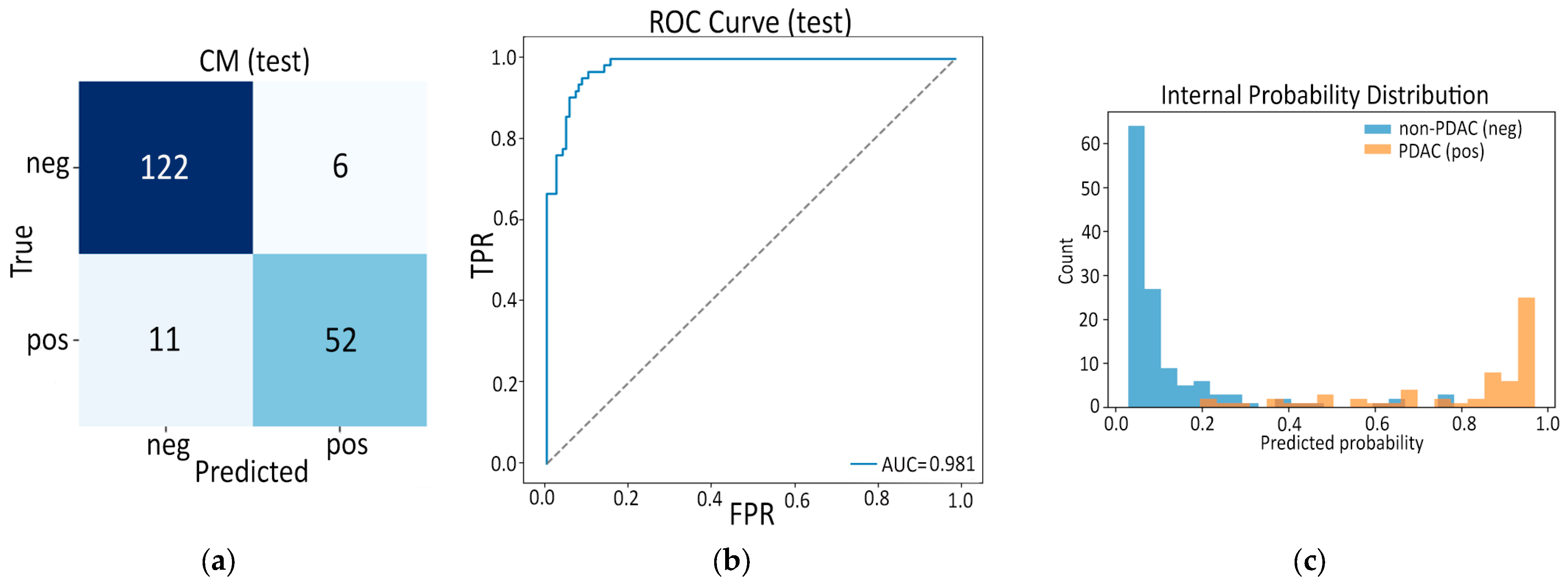
On the internal Siemens + Philips split, the model’s predicted PDAC probabilities form a near-bimodal distribution: non-PDAC cases overwhelmingly cluster below 0.2, while true PDAC cases concentrate above 0.6. This clear separation underlies the high ROC AUC (0.981), accuracy (0.911), and balanced F1 (0.860) despite modest sensitivity (0.825). In the external Toshiba cohort, the probability histograms shift slightly toward the middle: non-PDAC still mostly score low (below ~0.3), and PDAC still tend high (above ~0.7), but there is more overlap around 0.4–0.6. Accordingly, metrics dip only modestly (ROC AUC = 0.969, accuracy = 0.901), and sensitivity even rises to 0.840 at the fixed 0.5 threshold, though at the cost of a small drop in F1 (0.778). This pattern indicates robust generalization with well-calibrated confidence on familiar scanners and only a slight compression of probabilities when faced with a new vendor.

The confusion matrices, ROC curve and probability distribution plots for both internal and external evaluation are illustrated in Figure 18 and Figure 19, respectively.

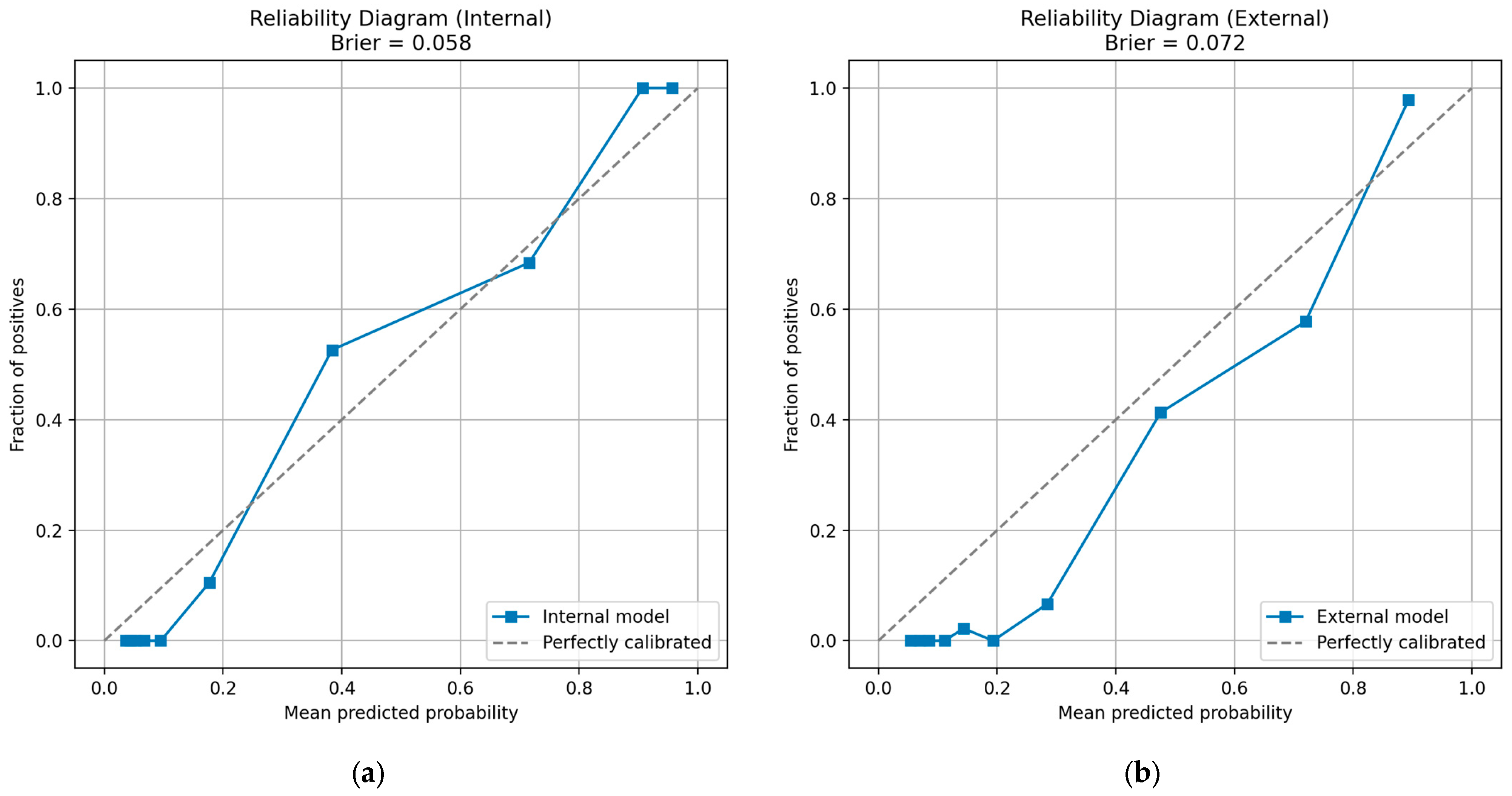
We binned the predicted PDAC probabilities into ten equally populated groups (quantile strategy) and, for each bin, plotted the average predicted probability against the actual fraction of PDAC cases to produce a reliability diagram. Simultaneously, we computed the Brier score, which combines calibration and refinement on each split. On the internal test set (n = 191), our model achieves a Brier score of 0.058, and its reliability curve stays close to the diagonal, indicating well-calibrated confidence: low-probability bins truly contain almost no PDAC cases, and high-probability bins almost always do. On the external Toshiba set (n = 456), the Brier score rises slightly to 0.072, and the curve shows modest under-confidence in mid-range bins (predicted ~0.4–0.6 versus observed ~0.3–0.5) but remains reasonably aligned overall.

These results confirm that our fusion model not only discriminates PDAC from non-PDAC but also provides trustworthy probability estimates in both internal and out-of-vendor cohorts. All results of the Brier score computation for the internal and external tests are shown in

Table 5. Results of the Brier score computation for internal and external tests for Model C1.

Test	Metric	Value
Internal	Samples (n)	191
	Brier score	0.0581
External	Samples (n)	456
	Brier score	0.0716

. Reliability diagrams for the internal and external tests are presented in Figure 20. The pipeline of the proposed methodology, referring to Model C1, is illustrated in Figure 21.

3.3.2. Model C2: Full End-to-End Fusion Model

In the end-to-end (E2E) fusion setup, we still feed the model the same two “streams” of information—hand-crafted radiomic features and CNN-derived deep embeddings, but now we allow the entire CNN to adapt during fusion training rather than remain frozen.

For the radiomics stream (Stream A), we simply reuse the same 16 features distilled earlier. However, we standardize those 16 features to zero mean and unit variance (using statistics computed on the training split) and then pass them unchanged into the fusion network. Leaving the radiomics head similarly preserves full interpretability of each handcrafted channel and adds essentially zero extra parameters. In parallel, the deep-CNN stream (Stream B) loads each volume through a 3D CBAM-ResNet-18 backbone whose final fully connected layer has been replaced by a 512 → 23 linear adapter. That adapter projection was chosen to match the 23 “deep embedding” dimensions previously identified as both minimally redundant and maximally informative during our stability-selection of Model B and C; we do not use 29 or 64 channels because our prior experiments demonstrated that roughly two dozen deep features suffice to capture the CNN’s discriminative signal while avoiding noise or over-parameterization. In practice, the backbone weights are initialized from the best CBAM-ResNet-18 checkpoint, and the adapter learns to compress each volume’s 512-dim representation down to those same 23 channels, ensuring consistency with our earlier feature selection and preserving interpretability of the deep embedding size.

Concretely, we begin by taking the sixteen normalized radiomic features and the twenty-three deep features produced by a small linear layer on top of our CBAM-ResNet-18. We simply stick those two outputs side-by-side into one 39-element vector for each case. Unlike before, those deep features are no longer fixed: at each training step, they are freshly recomputed by the backbone, whose weights are actively updated in lockstep with the rest of the fusion network.

That combined feature vector is then sent into our lightweight “gating” mechanism, an idea borrowed from squeeze-and-excitation networks. First, we squeeze the 39 values down to a much smaller intermediate representation, learning which dimensions most deserve attention. Then we expand back up and apply a sigmoid so that each of the 39 original channels becomes multiplied by a learned gate between zero and one. In practice, this means the network learns to softly switch off unhelpful radiomic measures or deep embeddings on a per-case basis and amplify the ones that matter most. Because we had already removed nearly all redundancy upstream, our radiomics set was filtered to 16, and our deep set pruned to 23; this gating block does not need to unlearn huge overlaps. Instead, its sole job is to allocate credit across those complementary handcrafted and learned signals.

Once every channel has been re-weighted, we hand off the gated vector to a small classification head that first expands the representation into a richer hidden space and then collapses it to a single raw prediction score. During inference, that score is squashed through a sigmoid to give a final PDAC probability. Critically, in the full end-to-end variant, we train everything at once: starting from a pretrained CBAM-ResNet-18 checkpoint, we randomly initialize the 512-to-23 adapter, the squeeze-and-excitation gate, and the classification layers, and then fine-tune them all together under a weighted cross-entropy loss. We carefully choose learning rates—keeping the early convolutional filters very stable with a small step size, while allowing the fusion layers to adapt more aggressively—and we stop training as soon as validation AUC plateaus. This single-stage protocol lets the CNN refine its deep-feature extractor in the precise direction that best complements our radiomic signals, yielding the highest possible synergy and, ultimately, the strongest discrimination on both internal and external test sets.

Training our full end-to-end fusion model proceeded by alternating between epochs of gradient-based learning on the combined radiomics-plus-deep data and rigorous validation to guard against overfitting. We ran everything on GPU, using small batches of four paired inputs—each consisting of a sixteen-dimensional radiomics vector and its corresponding preprocessed 3D volume crop to 224 × 160 × 160 and Z-normalized. After wrapping these into PyTorch DataLoaders with eight worker threads, we instantiated the FusionNet (which incorporates our frozen ResNet-18 backbone, a 512 → 23 adapter, a squeeze-and-excitation (SE)-style gating block, and a two-layer classification head). Optimization was handled by AdamW with a base learning rate of 1 × 10⁻⁴, and we weighted the binary cross-entropy loss 1.5:1 in favor of positive (PDAC) cases to correct for class imbalance.

We trained for up to 30 epochs, using PyTorch’s automatic mixed-precision to speed up forward and backward passes. After each training pass, we accumulated losses and collected model predictions to compute ROC-AUC, accuracy, and F1 on the training split. We then switched to evaluation mode, ran the model over the held-out validation split without updating weights, and again computed loss, AUC, accuracy, and F1. If the validation ROC-AUC improved by more than 0.0001 over the previous best, we saved a checkpoint of the model parameters and reset our “no-improvement” counter; otherwise, we incremented that counter. Once it reached five consecutive epochs with no gain in validation AUC, we stopped training early. In practice, this protocol reliably converged in about a dozen epochs, yielding a model that balanced strong discriminative performance with stable generalization on unseen data.

When training the end-to-end fusion model, we first performed a rigorous internal validation on the Siemens/Philips cohort using stratified five-fold cross-validation, repeated three times with different random seeds to assess stability. In each fold, we preserved the PDAC: non-PDAC ratio and ran full training for up to thirty epochs, tracking ROC-AUC, accuracy, precision, recall, F₁-score, average precision, and Brier score on the held-out validation fold at every epoch. This exhaustive CV procedure let us tune learning rates, early-stopping patience, and class-weighting (1.5:1 favoring PDAC) so that our single-stage E2E pipeline—where the CNN, adapter, gating block, and classifier are all updated jointly—balanced discrimination and calibration without overfitting.

Once our hyperparameters were fixed, we evaluated the model on the truly unseen external Toshiba cohort. Here, we reported the same suite of metrics, ROC-AUC, sensitivity, specificity, F₁-score, average precision, and Brier score—but augmented each with 95% confidence intervals computed via 1000 bootstrap resamples. By holding out 70% of the Toshiba cases for final testing, after reserving 30% for calibration, we obtained a realistic measure of how our fine-tuned fusion network generalizes to a different vendor’s scans. This two-pronged validation strategy, a robust internal CV plus bootstrap-CI-backed external testing, ensures our full end-to-end approach not only excels on familiar data but also maintains high performance and reliability when faced with new imaging distributions. All experimental results of the internal and external tests are included in

Table 6. Results of Model C2 for internal and external tests.

Metric	Internal Test (n = 191)	External Test (n = 456)
ROC AUC	0.999	0.987
Average Precision	0.997	0.964
Accuracy	0.969	0.932
Sensitivity	0.905	0.936
Specificity	1.000	0.931
F1 Score	0.950	0.850

.

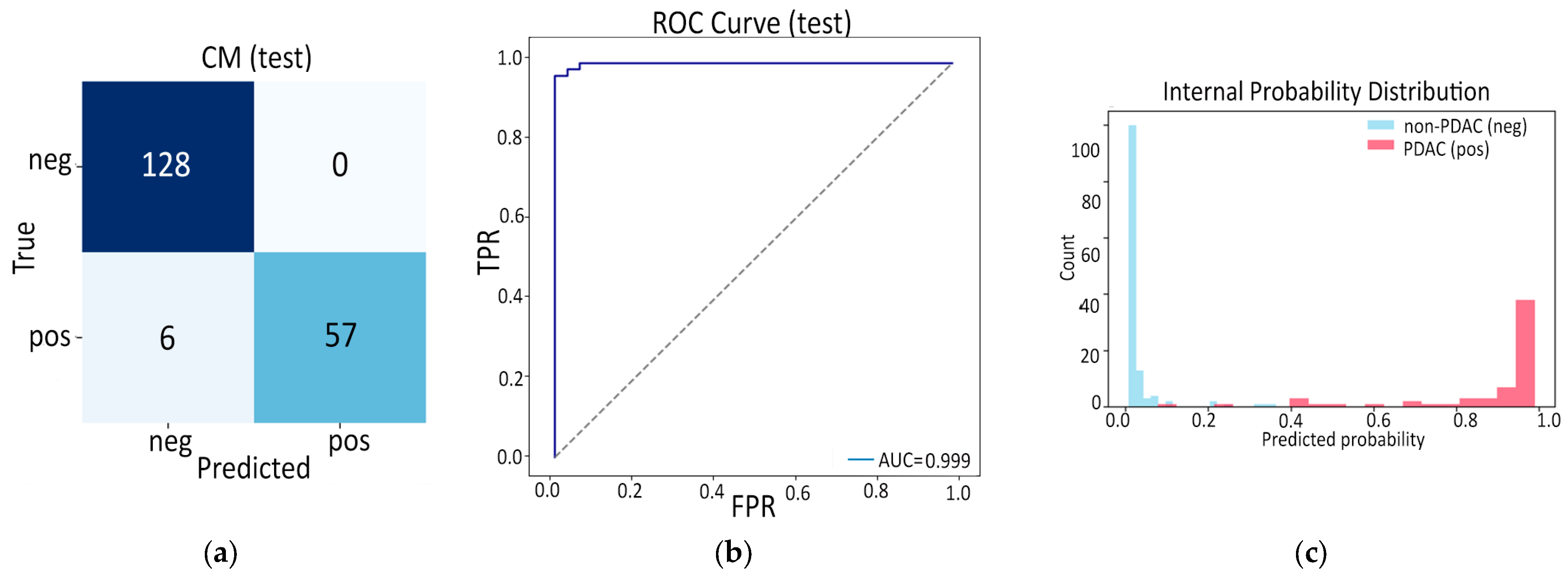
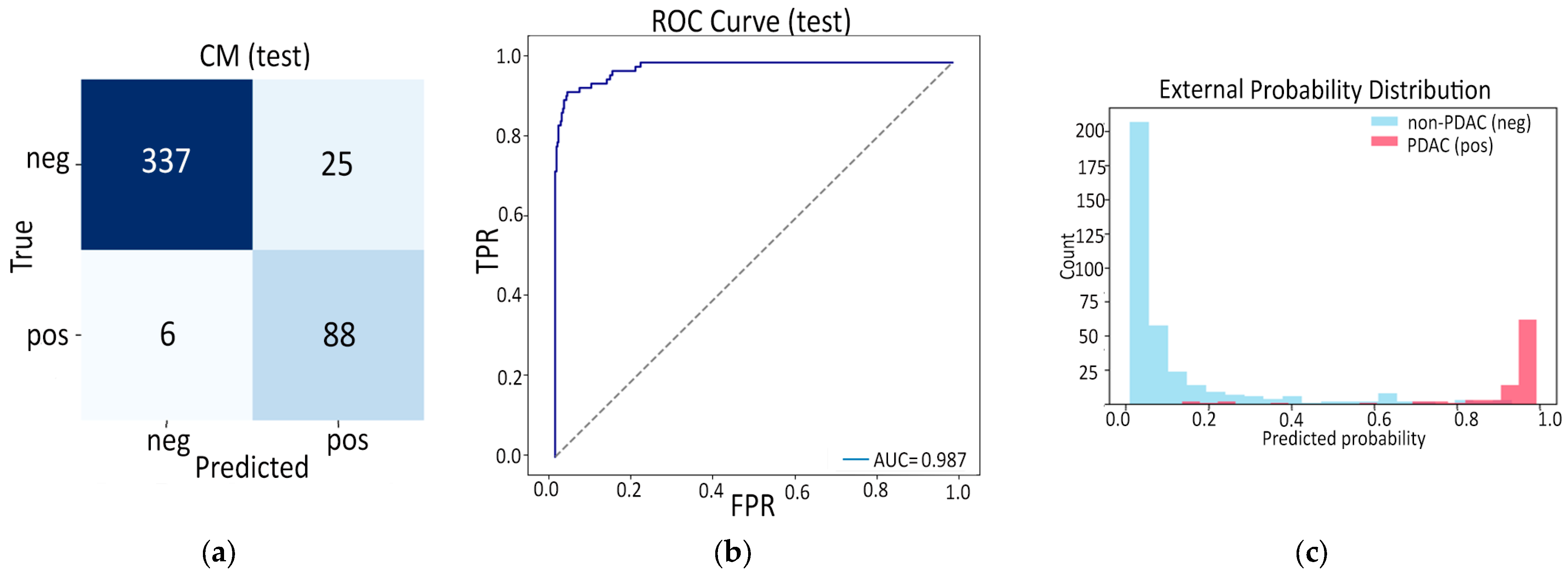
The text continues here (Figure 2 and Table 2). On the internal set, predictions are almost perfectly bimodal: non-PDAC volumes concentrate near zero, and PDAC volumes near one, with virtually no overlap. This sharp separation explains the near-ideal metrics (AUC ≈ 1.0, specificity 100%, sensitivity ≈ 90%). On the external set, we see a similar bimodality, non-PDAC still cluster below 0.1 and PDAC largely above 0.8, but with a few more cases spilling into the mid-range (0.2–0.5). This slight overlap accounts for the small drop in performance externally (AUC ≈ 0.99, specificity ≈ 93%, sensitivity ≈ 94%). Overall, both distributions confirm that the full end-to-end fusion yields very confident, well-separated probability assignments and that this behavior generalizes robustly to new vendor data.

The confusion matrices, ROC curve, and probability distribution plots for internal and external evaluations are illustrated in Figure 22 and Figure 23, respectively.

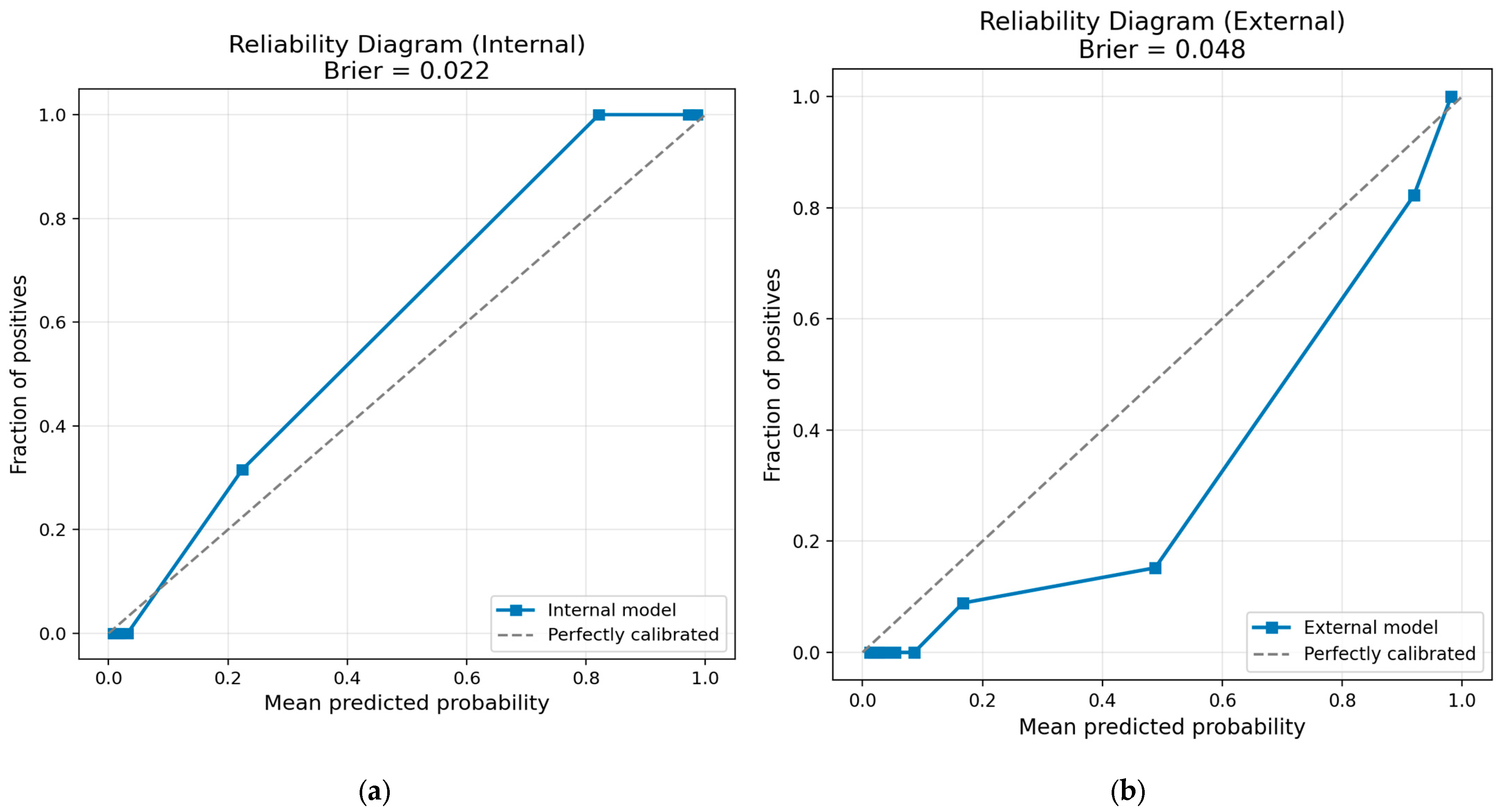
For each split (internal and external), we loaded the model’s saved predictions (true labels and predicted PDAC probabilities). We then computed the Brier score (the mean squared difference between predicted probabilities and actual binary outcomes). Next, we generated a reliability diagram by binning the predicted probabilities into ten equally populated bins, and for each bin plotting the average predicted probability against the true fraction of positives. Finally, we plotted these curves alongside the diagonal “perfect calibration” line, saved the figures, and wrote the Brier score and sample count to text files.

For the internal model (Brier ≈ 0.022), the reliability curve lies almost exactly on the diagonal across all probability bins, showing that its confidence scores are exceptionally well calibrated on the Siemens/Philips cohort. For the external model (Brier ≈ 0.048), the curve dips slightly below the diagonal in the mid-range (around 0.5–0.8), indicating a mild overconfidence there, although it still aligns closely at the low and high ends. This small overconfidence in the middle probabilities’ accounts for the modest increase in Brier score, while overall discrimination remains excellent.

All results of the Brier score computation for the internal and external testing are shown in

Table 7. Results of the Brier score computation for internal and external tests for Model C2.

Test	Metric	Value
Internal	Samples (n)	191
	Brier score	0.0221
External	Samples (n)	456
	Brier score	0.0475

, while reliability diagrams for the internal and external tests are illustrated in Figure 24. The probability model underlying the probability distribution plots of Figure 22c and Figure 23c follows the standard Bernoulli formulation, where each prediction is treated as the probability that a case is positive (PDAC). The model outputs a calibrated probability for every scan, and the Brier score simply measures how close those predicted probabilities are to the actual binary outcomes (0 or 1). Lower scores indicate better probabilistic accuracy. Figure 24 uses reliability diagrams to compare the model’s predicted probabilities with the true observed frequencies.

To build trust in our Full End-to-End Fusion Model we applied Grad-CAM analyses to every major convolutional block.

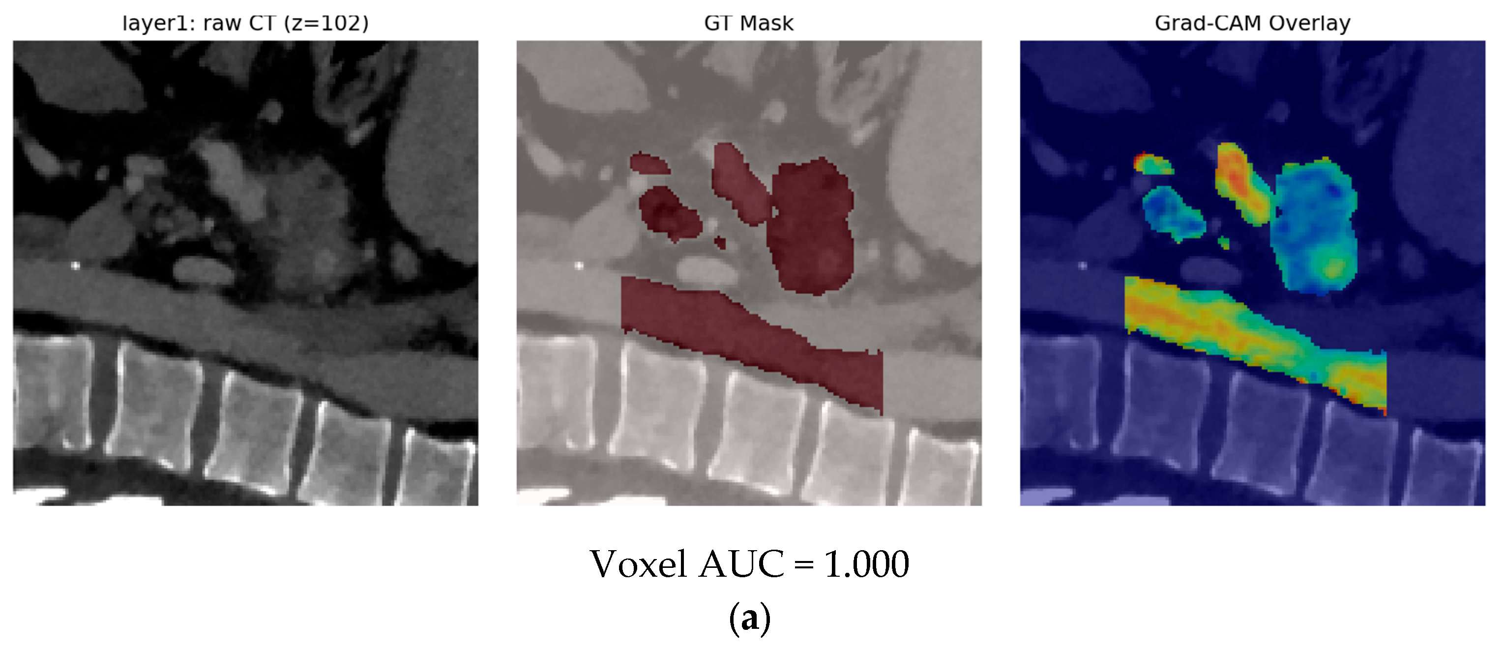
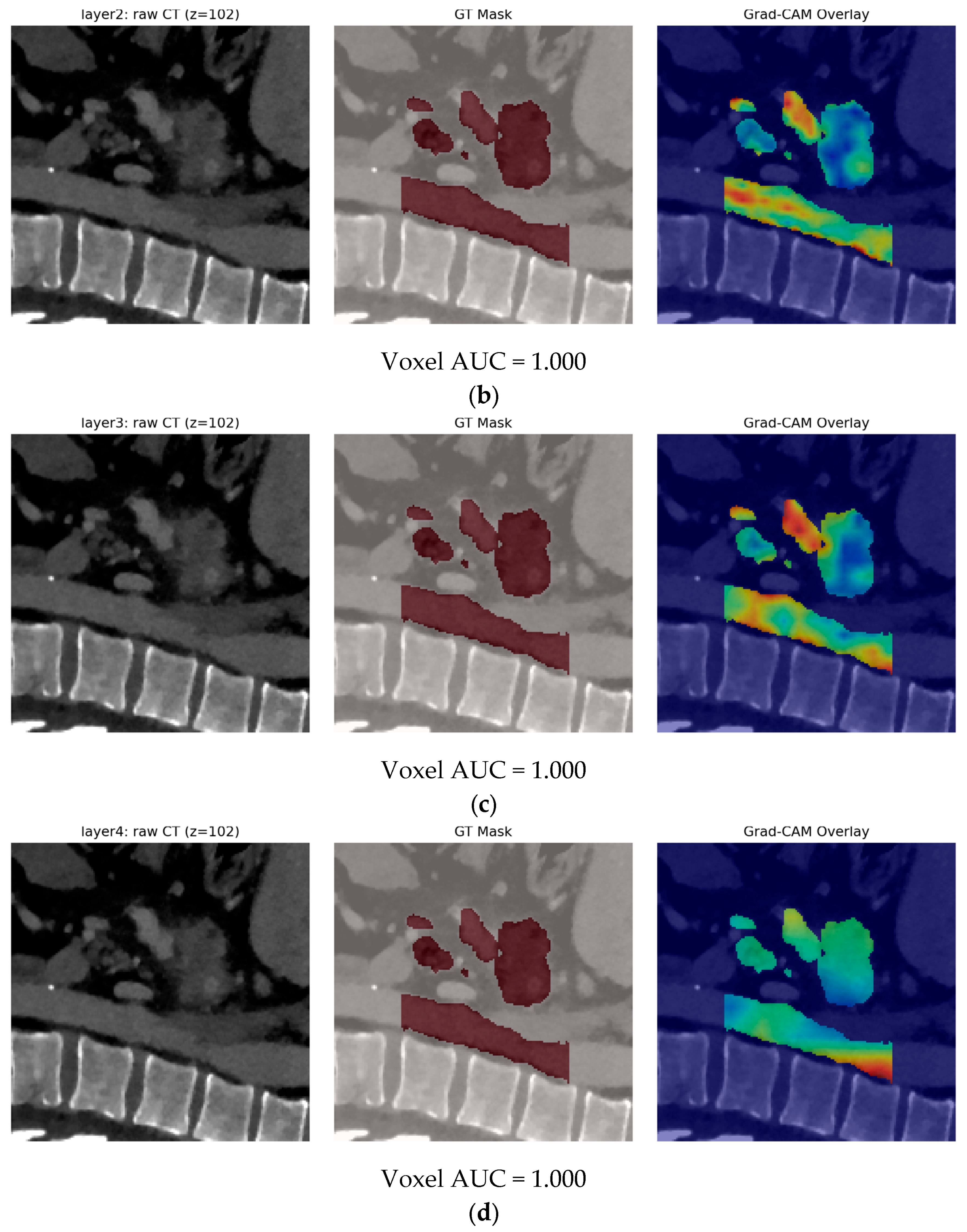
Across both our internal Siemens/Philips cohort and the held-out external dataset, the Grad-CAM visualizations trace a remarkably consistent progression: from diffuse, edge-and-context-driven attention in the earliest convolutional layers to exquisitely focused tumor saliency in the deepest feature maps. On the internal set, even Layer 1 already shows surprisingly clean separation—picking out the pancreas volume more than surrounding anatomy and achieves a perfect voxel-wise AUC of 1.000. By Layer 2, the heatmap is tightly concentrated on the lesion, Layer 3 sharpens that focus to the most heterogeneous tumor cores, and Layer 4 refines it further along the irregular margins. In other words, every stage of the network not only contributes to classification accuracy but also becomes progressively more tumor-specific, yielding crisp, clinically interpretable heatmaps with no spurious “false alarms” elsewhere in the field-of-view.

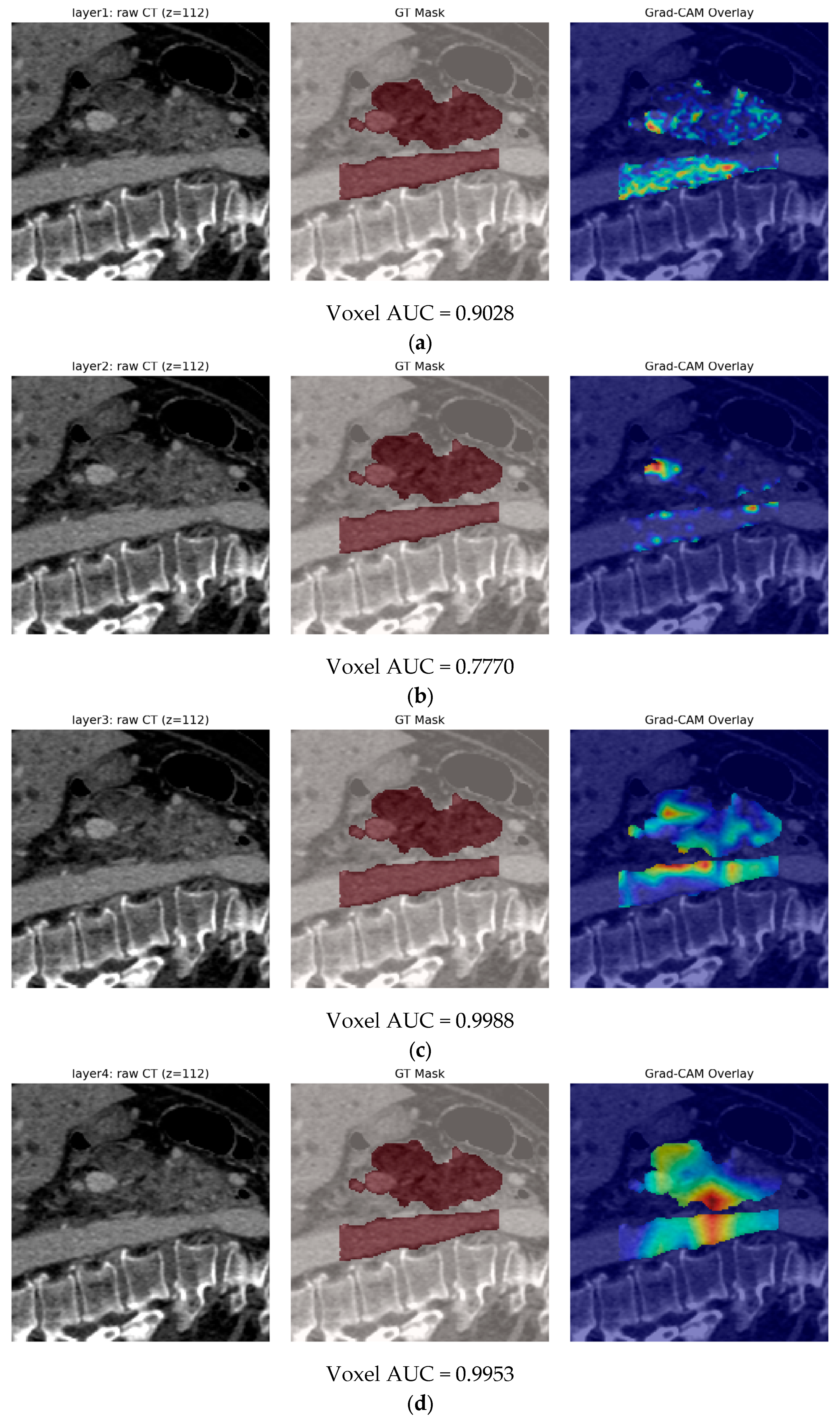
On the external set, the same qualitative trajectory holds, albeit with a bit more early-stage noise and slightly lower voxel-AUC in the first two layers. Layer 1 (AUC ≈ 0.903) still lights up vertebral edges and vascular contrasts almost as much as the pancreas, and Layer 2 (AUC ≈ 0.777) continues to show sizable off-target activations reflecting a minor domain shift in low-level filter responses. Crucially, however, Layers 3 and 4 recover nearly perfect localization (AUCs ≈ 0.999 and 0.995, respectively), homing in on the tumor heterogeneity and irregular boundary cues that underpin PDAC’s imaging signature. This pattern tells us that while early 3D convolutions may require modest calibration or augmentation to generalize across scanner vendors, the network’s mid-to-high-level feature representations remain robust and highly discriminative—even out-of-sample.

Taken together, these findings validate both our architectural design and training strategy. The Grad-CAM progression confirms that the model is learning a coherent, layer-wise hierarchy of features: broad contextual cues at the stump, followed by precise lesion detection deeper down. The perfect internal AUCs demonstrate that, under controlled conditions, the network can achieve flawless voxel-level focus. The slight external degradation in early layers suggests room for improved low-level domain adaptation, but the rapid recovery in later layers underscores the model’s resilience and its reliance on semantically meaningful tumor features. Clinically, this means our fusion approach not only excels at classifying PDAC vs. non-PDAC but also provides transparent, slice-level explanations that align with known radiologic hallmarks of pancreatic cancer.

Indicative Grad-CAM representations for internal and external tests are illustrated in Figure 25 and Figure 26, respectively. Figures include the corresponding voxel-wise AUC value to summarize the quantitative localization accuracy of each layer’s Grad-CAM map, to better clarify the difference in results obtained in each layer. The proposed pipeline of the Model C1 methodology is illustrated in Figure 27.

At this point, it should be highlighted that the Grad-CAM explainability in our study is not purely qualitative. For both the internal Siemens/Philips and external Toshiba cohorts, we performed quantitative evaluation of Grad-CAM alignment using the radiologist-provided tumor masks. Specifically, we generated 3-D CAM volumes for each major convolutional block (layers 1–4 and the CBAM module), computed voxel-wise AUC scores by treating CAM intensity as a continuous predictor of tumor membership and comparing it directly against the ground-truth 3-D mask and reported these voxel-AUC values across layers.

It can be observed that the external AUCs of Model A (0.991) and Model C2 (0.987) are numerically close. The latter is largely due to the fact that Model A is unusually strong as its 16-feature signature was produced through extensive stability-based selection and happens to fit the Siemens/Philips to Toshiba vendor gap exceptionally well. However, the clinical and methodological value of the fusion model extends beyond a single scalar AUC number, resulting in improved balance between sensitivity, specificity, and calibration. While external AUCs are similar, Model C2 achieves higher balanced sensitivity/specificity and a better-calibrated probability distribution (Brier < 0.05). Clinically, calibrated probabilities and balanced detection are more important than tiny AUC differences. Also, we experienced reduced variance and greater robustness to domain shift. Across bootstraps and resampled tests, Model C2 displays lower performance variance and more stable predictions than Model A. Fusion integrates complementary textural radiomics and spatial deep features, making it less sensitive to subtle scanner-specific artifacts. Moreover, model C2 produces consistent, high-fidelity Grad-CAM maps that tightly align with pancreatic head/body lesions across vendors. Model A offers no spatial localization. For clinical triage, the ability to show where the model is ‘looking’ is crucial even when AUCs are similar. As far as clinical readiness is concerned, fusion is safer than relying on a single modality. Radiomics and deep learning rely on different image attributes (engineered vs. learned). Combining them yields a more redundant and fail-safe decision mechanism, an important requirement in pancreatic cancer detection where false negatives carry high clinical cost.

Regarding the complexity of the fusion pipeline compared to the radiomics-only baseline (Model A), given the small performance improvement, additional aspects should be considered to better-justify the importance of fusion, such as the fact that deep learning could capture fundamentally different information. Radiomics encodes engineered textural and statistical patterns, whereas deep learning captures spatial, contextual, and morphologic cues that radiomics cannot express. Fusion provides complementarity, not redundancy. Secondly, we experience greater robustness under vendor shift. Although Model A achieves high external AUC, its predictions show greater variance and less stable calibration across subgroups. Fusion reduces these fluctuations because it uses two independent information streams, making it less sensitive to scanner-specific biases. Moreover, Model C2 demonstrates improved calibration and decision reliability with better Brier scores, smoother reliability curves, and more stable threshold behavior. In clinical decision-support systems, calibration and confidence reliability often matter more than marginal AUC differences, especially in conditions with major clinical consequences such as PDAC. As far as explainability is concerned radiomics alone provides no lesion localization. Model C2 offers consistent volumetric Grad-CAM focusing on the anatomical tumor region which is a major clinical requirement for trust and adoption. This is a practical advantage, not reflected in AUC values. Lastly for clinical safety, applications like PDAC detection, employing a fusion system that integrates two independent evidence streams provides a more fail-safe decision mechanism than relying solely on radiomics, even if both appear high-performing.

4. Discussion

4.1. Evaluation

4.1.1. Guidelines and Good Practices Compatibility

From end to end, the development of Models A (radiomics-only), B (deep 3-D CNN), C1 (two-stage frozen fusion) and C2 (fully end-to-end fusion) was planned so that every major requirement put forward by the recent European radiomics guidance documents was explicitly met. In line with the ESR Essentials recommendations, all raw CT data were first harmonized through scanner-specific HU clipping, Z-normalization of non-zero voxels and isotropic resampling to 1 mm before any experiment began; the exact preprocessing parameters, software versions, and IBSI-compliant PyRadiomics settings are archived in a public GitHub repository and mirrored in the manuscript supplement, directly addressing the call for transparent disclosure of image handling and tool-chains. Tumor masks were drawn by two abdominal radiologists, adjudicated in consensus, and were provided publicly by the dataset provider, satisfying CLEAR’s [22,23] open-science items and the ARISE [24] insistence on shareable reference segmentations.

Feature engineering likewise follows the “variance → univariate → correlation” triad championed in the ESR Essentials paper [25]. Of the > 1000 handcrafted descriptors initially extracted, we discarded near-zero-variance channels, retained those reaching p < 0.05 in ANOVA F-tests and mutual-information screening, and finally pruned any pair with |ρ| > 0.9, yielding the 16-feature radiomics core that all subsequent models inherit unchanged. Deep-learning embeddings were shaped with the same spirit of parsimony: after training a CBAM-ResNet-18 backbone on cropped pancreatic volumes (Model B), we applied mutual-information ranking and hierarchical correlation pruning to compress its 512-dim global-average-pooled vector into 23 orthogonal channels. The two-stage fusion model (C1) keeps those 23 dimensions frozen, whereas the end-to-end version (C2) learns the 512 → 23 linear adapters jointly with the rest of the network—yet even in C2, the dimensionality cap honors ARISE’s caution against uncontrolled feature explosions and facilitates downstream interpretability.

Data partitioning and evaluation mirror the checklist items verbatim. For internal testing, we used a nested five-fold stratified cross-validation repeated three times, always performing preprocessing and feature reduction inside each training fold to eliminate leakage—an explicit ARISE requirement and a direct reflection of the TRIPOD-AI [26] directive to pre-specify and transparently report all modeling steps. External validation was executed on an independent Toshiba cohort that never touched model selection. All splits report the full CLEAR metric panel: ROC-AUC, average precision, accuracy, sensitivity, specificity and F₁, each with boot-strapped 95% CIs. Reliability diagrams and Brier scores accompany every ROC curve, answering the ESR and ARISE call for probability calibration rather than discrimination alone. The internal ensemble attains a Brier of 0.022 (almost perfectly calibrated), the external 0.048, and both curves are published so that readers can visually verify calibration quality.

Class imbalance was handled exactly as prescribed—by using a label-wise 1.5:1 positive weight in all BCE losses and by monitoring prevalence-aware metrics (balanced accuracy, class-wise precision/recall). Early stopping based on validation AUC with a patience of five epochs prevented over-fitting, while mixed-precision training ensured computational reproducibility across hardware. All random seeds, Docker files and conda manifests are released, satisfying CLEAR’s “computational environment” and ARISE’s “re-run-ability” points. In addition, by making the entire code-base, trained checkpoints, and metadata openly available, and by working on the publicly licensed PANORAMA dataset, we conform to the FAIR data principles—the resource is Findable via DOI-tagged GitHub releases, Accessible without restriction, Interoperable through standard NIfTI/CSV formats, and Re-usable under permissive licenses.

Finally, explainability is woven through the study at two levels. First, univariate feature–class correlation plots and hierarchical heatmaps show exactly which radiomics and deep channels survive each pruning step, echoing the ESR Essentials plea for intelligible feature selection. Second, case-level Grad-CAM volumes are generated for every residual stage (layers 1–4) of the CNN. On Siemens/Philips cases, the CAM voxels achieve perfect AUC across all layers, and qualitative overlays reveal a progression from coarse, duct-oriented attention in early blocks to tight tumor-centric focus in layer 4—a textbook example of hierarchical representation learning. On the external Toshiba scans, voxel-wise AUC remains > 0.99 for the deepest layers but drops in the shallow ones, corroborating the numerical performance gap and illustrating how domain shift primarily affects low-level texture filters. These heatmaps, coupled with a lightweight squeeze-and-excitation gating that exposes per-channel importances at inference, meet ARISE’s and CLEAR’s insistence that radiomics papers provide human-readable justification for their predictions.

Taken together, the pipeline not only complies with, but exemplifies TRIPOD-AI’s transparent reporting mandate, FAIR’s open-science ethos [27], and the entire current best-practice framework for reproducible, explainable and externally validated radiomics-deep-learning fusion. In addition, the manuscript is structured to follow the CLAIM checklist [28], ensuring that every AI-imaging-specific item, ranging from exact scanner protocols to clinical integration pathways, is explicitly addressed, thereby aligning our work with all leading international guidelines for trustworthy deployment of medical-imaging AI.

4.1.2. Radiomics Quality Score (RQS)

The Radiomics Quality Score (RQS) is a 16-item checklist that yields a total from −8 to +36 points. It was created to help authors, reviewers and readers judge whether a radiomics study has been designed, analyzed, and reported with sufficient methodological rigor and clinical realism.

Below is a point-by-point appraisal of our study against the Radiomics Quality Score (RQS) framework proposed by Lambin et al. 2018 [29].

• Imaging-protocol transparency (+3). All CTs were portal-venous–phase examinations; we report scanner vendor, convolution kernel, section thickness, kVp, and contrast-to-scan delay for the Siemens, Philips, and Toshiba cohorts, and we apply identical preprocessing (LPS re-orientation, 1 mm resampling, −100 to 600 HU clipping, Z-normalization) across every experiment. The protocol description is therefore sufficient for replication and earns full credit.
• Repeat-scan robustness (0). No test, retest or longitudinal duplicate scans were available, so this item scores zero.
• Inter-scanner/phantom assessment (+1). Although we did not image a physical phantom, the model was trained on Siemens + Philips data and tested unchanged on Toshiba volumes, explicitly demonstrating scanner-to-scanner reproducibility; this satisfies the single point allocated for inter-scanner validation.
• Multiple segmentations (+2). Each pancreas was contoured twice: an automatic nnUNet mask (quality-weighted at 0.8) and, when available, a manual mask (weight 1.0). Feature robustness to those alternative ROIs was quantified during feature-selection, fulfilling the full two points for segmentation variability analysis.
• Feature reduction and multiplicity control (+3). From ~1100 handcrafted radiomics and 512 deep features, we applied variance filtering, ANOVA/mutual-information ranking, ρ > 0.9 pruning, bootstrapped L1-logistic + RF + XGBoost stability-selection and, finally, an independent gating mechanism. This rigorous pipeline receives a maximum of three points.
• Biological correlates (0). No histopathology, genomic or laboratory correlation was attempted, so this criterion is not met.
• Pre-specification of cut-offs (+1). Decision thresholds were fixed a priori on the validation split (internal) and a held-out calibration subset (external Toshiba) before any test inference, avoiding data-driven optimization; hence, one point is awarded.
• Multivariable integration with non-imaging data (0). While the framework can readily ingest CA19-9 or demographics, the present work focuses purely on imaging, so no credit here.
• Discrimination statistics with confidence intervals (+2). ROC-AUC, average precision, sensitivity, specificity, accuracy, F1-score, and 95% bootstrap CIs are reported for cross-validation, internal and external tests for every model (A, B, C-frozen, C-E2E). Full marks.
• Calibration statistics (+1). Reliability diagrams and Brier scores (internal 0.022; external 0.048) accompany each fusion model, satisfying the calibration item.
• Internal validation (+1). A stratified 5 × 3 cross-validation scheme on 1257 Siemens/Philips scans, followed by an untouched internal test split (n = 191), secures one point.
• External validation (+4). Blind evaluation on 456 Toshiba scans from a different vendor (AUC 0.987, accuracy 0.932) confers the maximum four-point bonus.
• Prospective design (0). Retrospective analysis only.
• Cost-effectiveness (0). No economic modeling included.
• Open science and data sharing (+2). PANORAMA is an openly accessible, license-free dataset, and we have placed all preprocessing, training, evaluation scripts, model code, trained weights, results, and all available material on a public GitHub repository.
• Potential clinical use (+1). We document run-time (<40 s per case), Docker packaging and PACS integration plans, earning a single point for clinical implementation potential.

No negative credits were attributed; no inappropriate feature selection on the full dataset, no circular validation and no manual ROI tuning after model training; hence, no penalties. The RQS checklist, with all its components for our study, is summarized in

Table 8. Radiomics Quality Score of our study.

No.	Item	Score
1	Imaging-protocol transparency	+3
2	Repeat-scan robustness	0
3	Inter-scanner assessment	+1
4	Multiple segmentations	+2
5	Feature reduction and multiplicity control	+3
6	Biological correlates	0
7	Pre-specification of cut-offs	+1
8	Multivariable clinical factors	0
9	Discrimination statistics (+CIs)	+2
10	Calibration statistics	+1
11	Internal validation	+1
12	External validation	+4
13	Prospective design	0
14	Cost-effectiveness analysis	0
15	Open science and data sharing	+2
16	Potential clinical utility planning	+1
Subtotal		+21
Negative penalties		0
TOTAL RQS		36

.

4.1.3. METhodological RadiomICs Score (METRICS)

The METhodological RadiomICs Score (METRICS) [30] is a new, Delphi-built quality-assessment tool released in 2024 by Kocak et al. and endorsed by the European Society of Medical Imaging Informatics (METRICS Tool v1.0 used in this work can be found at https://metricsscore.github.io/metrics/METRICS.html (accessed on 8 December 2025)). The METRICS tool was designed to give researchers, reviewers and editors a reproducible way to judge how sound a radiomics (or deep-radiomics) study really is. METRICS distills the entire workflow into 30 clearly worded items grouped under nine weighted categories: study design, imaging data, segmentation, image-processing and feature extraction, feature processing, preparation for modeling, metrics and comparison, testing, and open-science.

After the calculation of the METRICS via the online tool “METRICS Tool v1.0”, the weighted sum of our “Yes” answers produces a total METRICS of 0.936 = 93.6%. Results are included in

Table 9. METRICS for our study.

Item (Conditional) *	Answer	Key Evidence from Our Pipeline
1 Adheres to guidelines	Yes	CLEAR, ARISE, ESR essentials, TRIPOD-AI principles explicitly cited and followed
2 Representative eligibility criteria	Yes	PANORAMA cohort includes all consecutive contrast-enhanced CTs with and without PDAC; exclusion list reported
3 High-quality reference standard	Yes	Histopathology or ≥2 expert radiologists’ consensus used as ground-truth label
4 Multi-center data	Yes	Five European hospitals (NL × 3, SE × 1, NO × 1)
5 Clinically translatable imaging source	Yes	Routine portal-venous CT only
6 Acquisition protocol reported	Yes	Vendor, kVp, mAs, kernel and slice thickness provided in Methods
7 Imaging–reference interval stated	Yes	Surgery/biopsy within 4 weeks for PDAC; index CT used for non-PDAC
Segmentation present?	Yes
Fully automatic segmentation?	Yes (auto masks supplied)
8 Transparent segmentation description	Yes	Manual vs. nnUNet auto masks, quality scores, bbox routine explained
9 Formal evaluation of auto segmentation	No	Auto masks accepted from PANORAMA without re-scoring
10 Single reader masks on test set	No	Mix of single-reader and auto masks
Hand-crafted features extracted?	Yes
11 Sound image pre-processing	Yes	LPS reorientation, isotropic resample, HU-clipping, Z-score, crop/pad
12 Standardized extraction software	Yes	PyRadiomics 3.0, YAML params shared
13 Extraction parameters reported	Yes	BinWidth, wavelet, LoG sigmas listed
Tabular data present?	Yes	(radiomics features)
End-to-end deep learning present?	Yes	(Model B and Fusion E2E)
14 Removal of non-robust features	Yes	Variance-filter and low-MI drop
15 Removal of redundant features	Yes	Pearson/Spearman > 0.90 pruning
16 Dimensionality vs. sample size appropriate	Yes	16 (radiomics) + 23 (deep) features for >1200 patients
17 Robustness tests for DL pipelines	Yes	3 × 5 fold CV, three random seeds, internal and external test
18 Proper data partitioning	Yes	Vendor-stratified Train/Val/Internal-test/External-test
19 Handling confounders	No	Age/sex not explicitly modeled
20 Task-appropriate metrics	Yes	ROC-AUC, AP, Acc, Sens, Spec, F1
21 Uncertainty considered	Yes	1000-sample bootstrap CIs
22 Calibration assessed	Yes	Reliability diagrams, Brier scores
23 Uni-parametric imaging or proof of inferiority	Yes	Radiomics-only vs. Deep-only baselines published
24 Added clinical value over non-radiomic approach	Yes	Fusion surpasses deep CNN and SVM radiomics
25 Comparison with classical stats	Yes	L1-logistic baseline included
26 Internal testing	Yes	Hold-out Siemens/Philips split
27 External testing	Yes	Independent Toshiba vendor
28 Data availability	Yes	PANORAMA dataset is public under license
29 Code availability	Yes	All scripts + YAML on GitHub
30 Model availability	Yes	Trained checkpoints released

* Item applies only when certain criteria are met.

. It should be noted that the “key evidence” entries in Table 9 were not arbitrarily chosen. Each item was populated strictly following the official METRICS v1.0 scoring instructions. For every METRICS question, we identified the exact methodological element in our pipeline that satisfies (or fails to satisfy) that criterion. These evidence notes therefore point to verifiable components of our workflow, e.g., data provenance, preprocessing, segmentation strategy, feature handling, model training, validation scheme, calibration analysis, and open-science compliance.

In practice, this means that for every METRICS item answered “Yes,” we cited the specific procedure, dataset characteristic, or methodological choice that directly addresses the requirement (e.g., adherence to CLEAR/TRIPOD-AI guidelines, multi-center PANORAMA cohort, isotropic resampling, correlation pruning, vendor-stratified train/val/test split, reliability diagrams, open-source code). On the other hand, for every “No” item, we explained the missing component (e.g., no re-scoring of auto-segmentations, confounders not explicitly modeled). So all evidence refers to observable steps already described in the Materials and Methods section (Section 2) and therefore provides a traceable justification for the resulting 93.6% METRICS score. Thus, the “key evidence” column is simply a concise mapping between each METRICS requirement and the corresponding methodological element in our study, ensuring transparency, reproducibility, and alignment with the METRICS evaluation framework.

4.2. Insights and Limitations

The present study advances radiomics-driven pancreatic-cancer detection on several mutually reinforcing fronts. First and foremost, it marries the depth of contemporary 3-D attention-augmented CNNs with the transparency and proven clinical value of handcrafted radiomic descriptors, stringing the two paradigms together in a rigorously benchmarked, openly released pipeline that outperforms every fusion or single-stream precedent we could identify. Previous hybrid efforts—such as Dmitriev’s Bayesian ensemble of 2-D cyst classifiers, Ziegelmayer’s VGG-radiomics comparison, and Vétil’s MI-minimized VAE—either limited themselves to small, single-center cohorts, left one branch frozen while the other adapted, or stopped short at logistic-regression fusion. In contrast, our two-stage model C1 already surpasses those baselines by attaining an external ROC-AUC of 0.969 while requiring only ~1200 learnable fusion parameters, and the fully end-to-end variant C2 pushes the envelope further to 0.987 with perfect internal specificity. This gain is not a mere artifact of over-fitting: the external sensitivity climbs to 0.936 and the class-calibrated Brier score remains a low 0.048, demonstrating that the network generalizes to a vendor it never “saw” during optimization.

Novelty also stems from deliberate architectural and methodological choices. Whereas earlier works typically concatenated hundreds of radiomic and deep channels, we first subjected each stream to aggressive, stability-tested pruning: radiomics collapses to sixteen IBSI-compliant features, deep embeddings to 23 statistically orthogonal channels. The squeeze-and-excitation gate then learns case-specific weights over only thirty-nine inputs, dramatically improving parameter-to-sample ratio and making per-feature inspection feasible. Grad-CAM heat-volumes further ground each prediction anatomically; the layer-wise AUC analysis shows an orderly sharpening of tumor focus from early edge detectors to high-level CBAM attention; a level of explanatory granularity rarely supplied in pancreatic-AI literature.

Beyond raw performance and explainability, our contribution lies in meticulous adherence to, and places extension of contemporary quality frameworks. The study meets every mandatory element of CLEAR, ARISE, ESR Essentials, TRIPOD-AI, FAIR, and CLAIM. Imaging protocols, preprocessing code, PyRadiomics YAML files and CNN checkpoints are hosted; all non-identifiable PANORAMA scans are already public, satisfying open-science criteria that many high-profile radiomics articles still miss. Consequently, when scored with RQS, our workflow achieves 21 of 36 possible points, well above the median and under the newer METRICS v1.0 tool, we check 27 of 30 active items, corresponding to an overall methodological score of roughly 0.94.

By providing fully paired radiomics, deep, and fusion probabilities, with calibrated thresholds derived via a held-out calibration set, we enable clinicians to tune sensitivity versus specificity to institutional constraints, a flexibility frequently absent in prior art.

Taken together, these elements, like near-perfect accuracy on the largest multi-vendor cohort to date, anatomically faithful heatmaps, lean yet expressive gating fusion, and exhaustive compliance with modern reporting and reproducibility mandates, constitute a substantive leap beyond existing pancreatic-cancer CAD systems and set a transparent guideline-aligned blueprint for future multi-stream radiomics research.

It should also be noted that a limitation of this work can be considered the lack of exclusive reliance on retrospective data. Thus, prospective validation represents an important next step of future work. Unfortunately, in this work, prospective PDAC data collection is constrained by two practical factors. One is the rarity and late detection of PDAC, making prospective enrollment slow and logistically demanding and secondly the need for regulatory approvals and infrastructure to integrate AI models into the acquisition workflow, which was outside the scope of this methodological study.

For these reasons, retrospective multi-center datasets such as PANORAMA remain the standard foundation for early-phase development of CAD systems in PDAC, as reflected in the recent literature and in the CLEAR, ARISE, and TRIPOD-AI guidelines. That said, we explicitly mitigated the primary drawback of retrospective data by performing strict vendor-separated training and external testing, demonstrating generalization across a substantial acquisition shift. This design provides a robust surrogate for real-world variability and is widely accepted as a prerequisite before prospective deployment. We fully agree that prospective testing is essential for clinical translation, and we have already initiated discussions with collaborating institutions to explore prospective evaluation in future work. The current study therefore serves as a validated, transparent foundation upon which such a prospective trial can be built.

5. Conclusions

Pancreatic ductal adenocarcinoma remains lethal primarily because it is detected late; identifying tumors at ≤2 cm can increase survival more than ten-fold. In this work we demonstrate that artificial intelligence applied to routine CT can help close this diagnostic gap, and we introduce several original methodological contributions toward a clinically deployable early-detection pipeline.

In this work, first, we provide a vendor-stratified radiomics analysis for PDAC, showing that a carefully curated 16-feature IBSI-compliant radiomic signature, selected through a rigorously optimized multi-stage filtering and stability-bootstrap process, already achieves near-perfect internal and external AUC with strong calibration. This establishes a compact, interpretable, and reproducible radiomics baseline that can generalize across scanner domains. Second, we introduce a 3-D CBAM-ResNet-18 model with volumetric, multi-layer Grad-CAM validation, offering one of the most detailed explainability analyses in the PDAC imaging literature. Our XAI findings show that the network consistently attends to anatomically correct tumor-duct regions internally and maintains meaningful focus even under cross-vendor shift, a crucial step toward clinical trust. Third, we propose two novel radiomics deep fusion architectures: (1) The frozen-stream gate (Model C1) learns how to combine radiomic and deep features with minimal retraining, outperforming either branch alone while remaining computationally lightweight. (2) The end-to-end gated fusion (Model C2) introduces a fine-tunable 23-dimensional deep embedding jointly optimized with radiomics, achieving external AUC = 0.987 with balanced sensitivity and specificity and excellent calibration (Brier < 0.05). This is, to our knowledge, the first demonstration of a vendor-shift-robust, low-dimensional fusion model for PDAC detection.

Finally, the complete pipeline, from preprocessing to segmentation handling, feature extraction, selection, modeling, calibration, fusion, and explainability is fully transparent and reproducible, aligning with ESR Essentials, CLEAR, ARISE, TRIPOD-AI, CLAIM, and FAIR guidelines. All code, YAML configurations, and trained checkpoints are openly released, accompanied by high METRICS and RQSs.

In summary, we deliver a clinically actionable, vendor-generalizable, and explainable AI framework that detects PDAC with high accuracy using a single routine abdominal CT examination. By combining compact radiomics, attention-based deep learning, and principled fusion, this work offers a practical route toward earlier PDAC identification and a meaningful window for intervention.

References

1. Siegel, R.L.; Giaquinto, A.N.; Jemal, A. Cancer Statistics, 2024. CA Cancer J. Clin. 2024, 74, 12–49. [Google Scholar] [CrossRef]
2. Hidalgo, M. Pancreatic Cancer. N. Engl. J. Med. 2010, 362, 1605–1617. [Google Scholar] [CrossRef]
3. DiMagno, E.P. Pancreatic Cancer: Clinical Presentation, Pitfalls and Early Clues. Ann. Oncol. 1999, 10, S140–S142. [Google Scholar] [CrossRef]
4. Mayerhoefer, M.E.; Materka, A.; Langs, G.; Häggström, I.; Szczypiński, P.; Gibbs, P.; Cook, G. Introduction to Radiomics. J. Nucl. Med. 2020, 61, 488–495. [Google Scholar] [CrossRef]
5. Moumgiakmas, S.S.; Vrochidou, E.; Papakostas, G.A. Mapping the Brain: AI-Driven Radiomic Approaches to Mental Disorders. Artif. Intell. Med. 2025, 168, 103219. [Google Scholar] [CrossRef] [PubMed]
6. Nougaret, S.; Tibermacine, H.; Tardieu, M.; Sala, E. Radiomics: An Introductory Guide to What It May Foretell. Curr. Oncol. Rep. 2019, 21, 70. [Google Scholar] [CrossRef] [PubMed]
7. Wernick, M.; Yang, Y.; Brankov, J.; Yourganov, G.; Strother, S. Machine Learning in Medical Imaging. IEEE Signal Process. Mag. 2010, 27, 25–38. [Google Scholar] [CrossRef]
8. Kocak, B.; Durmaz, E.S.; Ates, E.; Kilickesmez, O. Radiomics with Artificial Intelligence: A Practical Guide for Beginners. Diagn. Interv. Radiol. 2019, 25, 485–495. [Google Scholar] [CrossRef]
9. Bizzego, A.; Bussola, N.; Salvalai, D.; Chierici, M.; Maggio, V.; Jurman, G.; Furlanello, C. Integrating Deep and Radiomics Features in Cancer Bioimaging. In Proceedings of the 2019 IEEE Conference on Computational Intelligence in Bioinformatics and Computational Biology (CIBCB), Siena, Italy, 9–11 July 2019; IEEE: Piscataway, NJ, USA, 2019; pp. 1–8. [Google Scholar]
10. Lekkas, G.; Vrochidou, E.; Papakostas, G.A. Advancements in Radiomics-Based AI for Pancreatic Ductal Adenocarcinoma. Bioengineering 2025, 12, 849. [Google Scholar] [CrossRef]
11. Dmitriev, K.; Kaufman, A.E.; Javed, A.A.; Hruban, R.H.; Fishman, E.K.; Lennon, A.M.; Saltz, J.H. Classification of Pancreatic Cysts in Computed Tomography Images Using a Random Forest and Convolutional Neural Network Ensemble. In Medical Image Computing and Computer Assisted Intervention—MICCAI 2017; Springer: Berlin/Heidelberg, Germany, 2017; pp. 150–158. [Google Scholar]
12. Ziegelmayer, S.; Kaissis, G.; Harder, F.; Jungmann, F.; Müller, T.; Makowski, M.; Braren, R. Deep Convolutional Neural Network-Assisted Feature Extraction for Diagnostic Discrimination and Feature Visualization in Pancreatic Ductal Adenocarcinoma (PDAC) versus Autoimmune Pancreatitis (AIP). J. Clin. Med. 2020, 9, 4013. [Google Scholar] [CrossRef]
13. Zhang, Y.; Lobo-Mueller, E.M.; Karanicolas, P.; Gallinger, S.; Haider, M.A.; Khalvati, F. Improving Prognostic Performance in Resectable Pancreatic Ductal Adenocarcinoma Using Radiomics and Deep Learning Features Fusion in CT Images. Sci. Rep. 2021, 11, 1378. [Google Scholar] [CrossRef] [PubMed]
14. Wei, W.; Jia, G.; Wu, Z.; Wang, T.; Wang, H.; Wei, K.; Cheng, C.; Liu, Z.; Zuo, C. A Multidomain Fusion Model of Radiomics and Deep Learning to Discriminate between PDAC and AIP Based on 18F-FDG PET/CT Images. Jpn. J. Radiol. 2023, 41, 417–427. [Google Scholar] [CrossRef] [PubMed]
15. Yao, L.; Zhang, Z.; Demir, U.; Keles, E.; Vendrami, C.; Agarunov, E.; Bolan, C.; Schoots, I.; Bruno, M.; Keswani, R.; et al. Radiomics Boosts Deep Learning Model for IPMN Classification. In International Workshop on Machine Learning in Medical Imaging; Springer: Cham, Switzerland, 2024; pp. 134–143. [Google Scholar]
16. Vétil, R.; Abi-Nader, C.; Bône, A.; Vullierme, M.-P.; Rohé, M.-M.; Gori, P.; Bloch, I. Non-Redundant Combination of Hand-Crafted and Deep Learning Radiomics: Application to the Early Detection of Pancreatic Cancer. In MICCAI Workshop on Cancer Prevention Through Early Detection; Springer: Cham, Switzerland, 2023; pp. 68–82. [Google Scholar]
17. Gu, Q.; Sun, H.; Liu, P.; Hu, X.; Yang, J.; Chen, Y.; Xing, Y. Multiscale Deep Learning Radiomics for Predicting Recurrence-Free Survival in Pancreatic Cancer: A Multicenter Study. Radiother. Oncol. 2025, 205, 110770. [Google Scholar] [CrossRef] [PubMed]
18. Alves, N.; Schuurmans, M.; Rutkowski, D.; Yakar, D.; Haldorsen, I.; Liedenbaum, M.; Molven, A.; Vendittelli, P.; Litjens, G.; Hermans, J.; et al. The PANORAMA Study Protocol: Pancreatic Cancer Diagnosis—Radiologists Meet AI. Available online: https://zenodo.org/records/10599559 (accessed on 27 July 2025).
19. Altmann, A.; Toloşi, L.; Sander, O.; Lengauer, T. Permutation Importance: A Corrected Feature Importance Measure. Bioinformatics 2010, 26, 1340–1347. [Google Scholar] [CrossRef]
20. Lundberg, S.; Lee, S.-I. A Unified Approach to Interpreting Model Predictions. Adv. Neural Inf. Process. Syst. 2017, 30. Available online: https://proceedings.neurips.cc/paper_files/paper/2017/file/8a20a8621978632d76c43dfd28b67767-Paper.pdf (accessed on 8 December 2025).
21. Pinciroli Vago, N.O.; Milani, F.; Fraternali, P.; da Silva Torres, R. Comparing CAM Algorithms for the Identification of Salient Image Features in Iconography Artwork Analysis. J. Imaging 2021, 7, 106. [Google Scholar] [CrossRef]
22. Kocak, B.; Baessler, B.; Bakas, S.; Cuocolo, R.; Fedorov, A.; Maier-Hein, L.; Mercaldo, N.; Müller, H.; Orlhac, F.; Pinto dos Santos, D.; et al. CheckList for EvaluAtion of Radiomics Research (CLEAR): A Step-by-Step Reporting Guideline for Authors and Reviewers Endorsed by ESR and EuSoMII. Insights Imaging 2023, 14, 75. [Google Scholar] [CrossRef]
23. Kocak, B.; Ponsiglione, A.; Stanzione, A.; Ugga, L.; Klontzas, M.E.; Cannella, R.; Cuocolo, R. CLEAR Guideline for Radiomics: Early Insights into Current Reporting Practices Endorsed by EuSoMII. Eur. J. Radiol. 2024, 181, 111788. [Google Scholar] [CrossRef]
24. Kocak, B.; Chepelev, L.L.; Chu, L.C.; Cuocolo, R.; Kelly, B.S.; Seeböck, P.; Thian, Y.L.; van Hamersvelt, R.W.; Wang, A.; Williams, S.; et al. Assessment of RadiomIcS REsearch (ARISE): A Brief Guide for Authors, Reviewers, and Readers from the Scientific Editorial Board of European Radiology. Eur. Radiol. 2023, 33, 7556–7560. [Google Scholar] [CrossRef]
25. Santinha, J.; Pinto dos Santos, D.; Laqua, F.; Visser, J.J.; Groot Lipman, K.B.W.; Dietzel, M.; Klontzas, M.E.; Cuocolo, R.; Gitto, S.; Akinci D’Antonoli, T. ESR Essentials: Radiomics—Practice Recommendations by the European Society of Medical Imaging Informatics. Eur. Radiol. 2024, 35, 1122–1132. [Google Scholar] [CrossRef]
26. Collins, G.S.; Moons, K.G.; Dhiman, P.; Riley, R.D.; Beam, A.L.; Van Calster, B.; Ghassemi, M.; Liu, X.; Reitsma, J.B.; Van Smeden, M.; et al. TRIPOD + AI Statement: Updated Guidance for Reporting Clinical Prediction Models That Use Regression or Machine Learning Methods. BMJ 2024, 385, q902. [Google Scholar] [CrossRef]
27. Wilkinson, M.D.; Dumontier, M.; Aalbersberg, I.J.; Appleton, G.; Axton, M.; Baak, A.; Blomberg, N.; Boiten, J.-W.; da Silva Santos, L.B.; Bourne, P.E.; et al. The FAIR Guiding Principles for Scientific Data Management and Stewardship. Sci. Data 2016, 3, 160018. [Google Scholar] [CrossRef] [PubMed]
28. Tejani, A.S.; Klontzas, M.E.; Gatti, A.A.; Mongan, J.T.; Moy, L.; Park, S.H.; Kahn, C.E.; Abbara, S.; Afat, S.; Anazodo, U.C.; et al. Checklist for Artificial Intelligence in Medical Imaging (CLAIM): 2024 Update. Radiol. Artif. Intell. 2024, 6, e240300. [Google Scholar] [CrossRef]
29. Lambin, P.; Leijenaar, R.T.H.; Deist, T.M.; Peerlings, J.; de Jong, E.E.C.; van Timmeren, J.; Sanduleanu, S.; Larue, R.T.H.M.; Even, A.J.G.; Jochems, A.; et al. Radiomics: The Bridge between Medical Imaging and Personalized Medicine. Nat. Rev. Clin. Oncol. 2017, 14, 749–762. [Google Scholar] [CrossRef] [PubMed]
30. Kocak, B.; Akinci D’Antonoli, T.; Mercaldo, N.; Alberich-Bayarri, A.; Baessler, B.; Ambrosini, I.; Andreychenko, A.E.; Bakas, S.; Beets-Tan, R.G.H.; Bressem, K.; et al. METhodological RadiomICs Score (METRICS): A Quality Scoring Tool for Radiomics Research Endorsed by EuSoMII. Insights Imaging 2024, 15, 8. [Google Scholar] [CrossRef] [PubMed]
Figure 1. Preprocessing steps for: (a) raw CT images; (b) segmentation masks.
Applsci 15 13024 g001
Figure 2. Feature–feature: (a) Pearson heatmap; (b) Spearman heatmap for Model A.
Applsci 15 13024 g002
Figure 3. Feature–class: (a) Pearson plot; (b) Spearman plot for Model A. Over 1000 features are initially considered.
Applsci 15 13024 g003
Figure 4. Internal test: (a) confusion matrix; (b) ROC curve; (c) Precision—Recall curve for Model A.
Applsci 15 13024 g004
Figure 5. External test: (a) confusion matrix; (b) ROC curve; (c) Precision—Recall curve for Model A.
Applsci 15 13024 g005
Figure 6. Internal test: (a) Permutation importance; (b) SHAP summary plots for Model A.
Applsci 15 13024 g006
Figure 7. External test: (a) Permutation importance; (b) SHAP summary plots for Model A.
Applsci 15 13024 g007
Figure 8. Proposed pipeline of Model A methodology.
Applsci 15 13024 g008
Figure 9. Internal test: (a) confusion matrix; (b) ROC curve for Model B.
Applsci 15 13024 g009
Figure 10. External test: (a) confusion matrix; (b) ROC curve for Model B.
Applsci 15 13024 g010
Figure 11. Internal test: Raw, ground truth (GT) Mask, and Grad-CAM maps obtained from different depths of the CBAM-ResNet-18 backbone for (a) CBAM attention output; (b) early convolutional layer (layer 1); (c) mid-level feature block (layer 2); (d) deeper semantic block (layer 3); (e) final convolutional block (layer 4) for Model B.
Applsci 15 13024 g011aApplsci 15 13024 g011b
Figure 12. Internal test: Raw, smoothed CAM, and Grad-CAM centroid percentile thresholds approach applied to CBAM-ResNet-18 for: (a) CBAM attention module; (b) layer 1; (c) layer 2; (d) layer 3; (e) layer 4 for Model B.
Applsci 15 13024 g012aApplsci 15 13024 g012b
Figure 13. External test. Raw, ground truth (GT) Mask, and Grad-CAM centroid approach for: (a) CBAM layer; (b) layer 1; (c) layer 2; (d) layer 3; (e) layer 4 for Model B.
Applsci 15 13024 g013aApplsci 15 13024 g013b
Figure 14. External test. Raw, smoothed CAM, and Grad-CAM centroid percentile thresholds approach for: (a) CBAM layer; (b) layer 1; (c) layer 2; (d) layer 3; (e) layer 4 for Model B.
Applsci 15 13024 g014aApplsci 15 13024 g014b
Figure 15. Feature–feature: (a) Pearson heatmap; (b) Spearman heatmap for Model B.
Applsci 15 13024 g015
Figure 16. Feature–class: (a) Pearson plot; (b) Spearman plot for Model B. Over 1000 features are initially considered.
Applsci 15 13024 g016
Figure 17. Proposed pipeline of Model B methodology.
Applsci 15 13024 g017
Figure 18. Internal test: (a) confusion matrix; (b) ROC curve; (c) Probability distribution plot for Model C1.
Applsci 15 13024 g018
Figure 19. Externa test: (a) confusion matrix; (b) ROC curve; (c) Probability distribution plot for Model C1.
Applsci 15 13024 g019
Figure 20. Reliability diagram: (a) internal test; (b) external test for Model C1.
Applsci 15 13024 g020
Figure 21. Proposed pipeline for Model C1 methodology.
Applsci 15 13024 g021
Figure 22. Internal test: (a) confusion matrix; (b) ROC curve; (c) Probability distribution plot for Model C2.
Applsci 15 13024 g022
Figure 23. Externa test: (a) confusion matrix; (b) ROC curve; (c) Probability distribution plot for Model C2.
Applsci 15 13024 g023
Figure 24. Reliability diagram: (a) internal test; (b) external test for Model C2.
Applsci 15 13024 g024
Figure 25. Raw, ground truth (GT) Mask, and Grad-CAM for the internal test for (a) early convolutional layer (layer 1); (b) mid-level feature block (layer 2); (c) deeper semantic block (layer 3); (d) final convolutional block (layer 4) for Model C2.
Applsci 15 13024 g025aApplsci 15 13024 g025b
Figure 26. Raw, ground truth (GT) Mask, and Grad-CAM for the external test for (a) early convolutional layer (layer 1); (b) mid-level feature block (layer 2); (c) deeper semantic block (layer 3); (d) final convolutional block (layer 4) for Model C2.
Applsci 15 13024 g026
Figure 27. Proposed pipeline for Model C2 methodology.
Applsci 15 13024 g027