Article

A 3D CNN Prediction of Cerebral Aneurysm in the Bifurcation Region of Interest in Magnetic Resonance Angiography

Medical Artificial Intelligence Laboratory, Division of Digital Healthcare, College of Software and Digital Healthcare Convergence, Yonsei University, Wonju 26493, Republic of Korea
*
Author to whom correspondence should be addressed.
These authors contributed equally to this work.
Appl. Sci. 2025, 15(24), 13004; https://doi.org/10.3390/app152413004
Submission received: 30 October 2025 / Revised: 30 November 2025 / Accepted: 8 December 2025 / Published: 10 December 2025
(This article belongs to the Special Issue Advanced Techniques and Applications in Magnetic Resonance Imaging)

Abstract

Quantitative vascular analysis involves the measurements of arterial tortuosity and branch angle in a region of interest in cerebral arteries to assess vascular risks associated with cerebral aneurysm. The measurements themselves are not a simple process since they are made on the three-dimensional (3D) structures of the arteries. The aim of this study was to develop a deep convolutional neural network (CNN) model to predict a probability score of aneurysm without direct measurements of the artery’s geometry. A total of 204 subjects’ image data were considered. In all, 585 gray-scale three-dimensional (3D) patches with the bifurcations near the center of the patches were extracted and labeled as either an aneurysm or a non-aneurysm class. Three-dimensional CNN architectures were developed and validated for the binary classification of the 3D patches. Accuracy, precision, recall, F1-score, receiver operating characteristics area under the curve (ROC-AUC), and precision recall AUC (PR-AUC) were calculated for test data. Deep learning predictions were compared with vessel geometry measurements. Deep learning probability scores were dichotomized into high-score and low-score groups. For both groups, bifurcation angles and sum-of-angles-metric (SOAM) were calculated and compared. ResNetV2_18 with translation as data augmentation achieved the highest mean ROC-AUC (0.735) and PR-AUC (0.472). The independent t-test indicated that for the bifurcation angle sum feature there was a statistically significant difference (t = −2.280, p-value < 0.05) between the low-score and the high-score groups. In conclusion, we have demonstrated a deep learning-based approach to the prediction of aneurysmal risks in the bifurcation regions of interest. Deep learning predictions were associated with vessel geometry measurements. This suggests that deep learning on 3D patches centered around the bifurcations has the potential to screen bifurcations with a high aneurysm risk.

1. Introduction

Cerebral aneurysms occur in 3–5% of the population and are characterized by the bulging of a blood vessel due to the weakening of its wall under blood flow pressure [1,2]. They are known to be associated with vascular morphology, hemodynamics, and clinical information such as aging, hypertension, smoking, and family history [3]. The detection of unruptured cerebral aneurysms increases with the aid of a noninvasive angiography, often during routine health checkups [4]. If left undiagnosed and untreated, the bulging vessel wall may rupture, leading to a subarachnoid hemorrhage, which can result in severe disabilities or even death [5].
Unruptured cerebral aneurysms are non-invasively identified with the aid of medical imaging, including intra-arterial digital subtraction angiography (DSA), computed tomography angiography (CTA), and magnetic resonance angiography (MRA). Identifying aneurysms in vascular images is critical, and neuroradiologists meticulously search for the location and presence of even minute aneurysms through extensive image analysis. Recently, artificial intelligence (AI) methods for automatically detecting cerebral aneurysms have been proposed in [6,7,8,9]. The methods primarily relied on U-Net segmentation models which were trained on labeled aneurysm masks. The inference procedure predicted aneurysm masks, leading to the detection of cerebral aneurysms from a full field-of-view of the cerebral angiography.
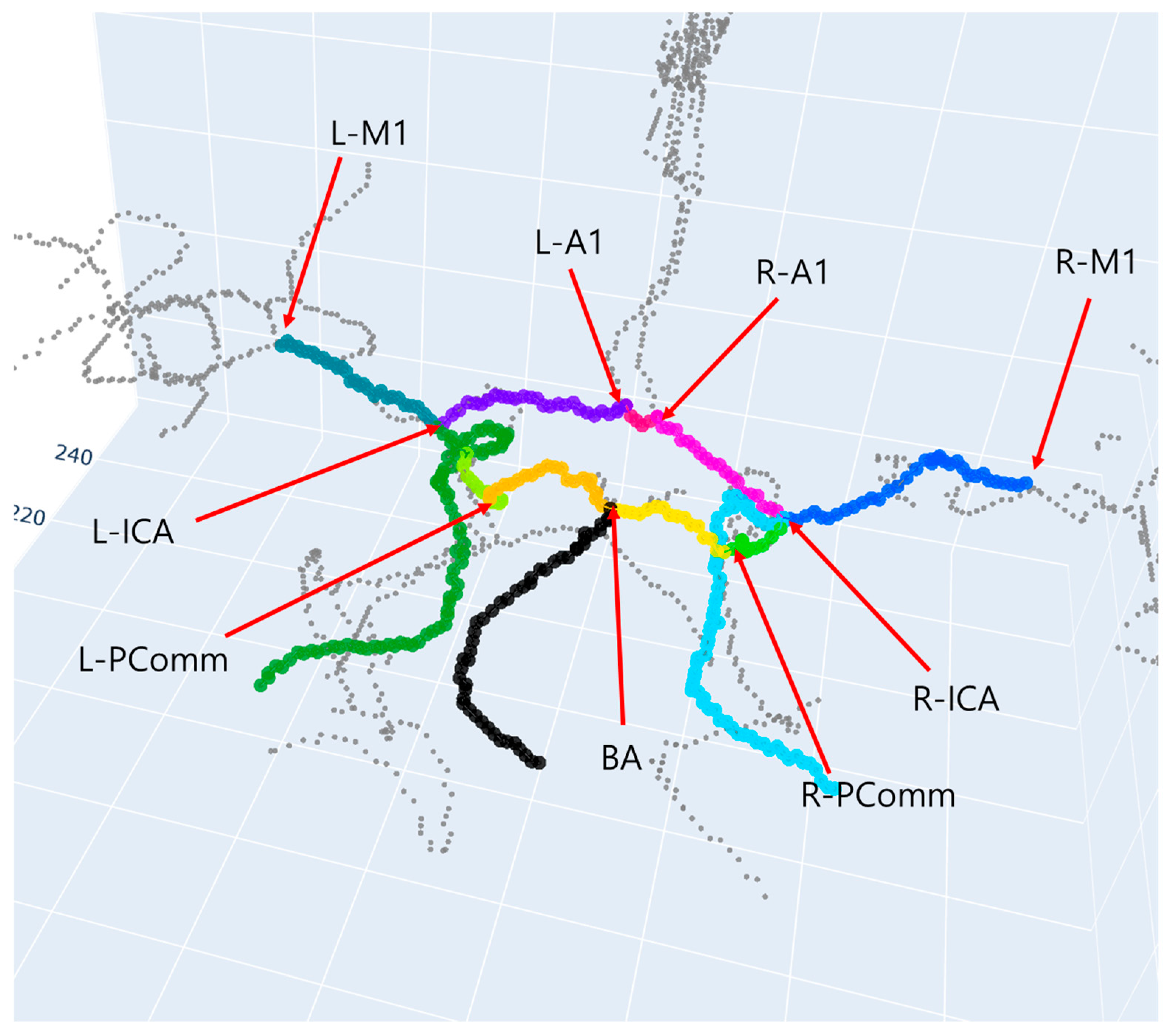
Research has demonstrated a correlation between the geometric characteristics of intracranial arteries and the development of cerebral aneurysms, although age and sex were associated with aneurysms. Cerebral aneurysms often occur at arterial bifurcations in the circle of Willis (CoW) [10]. Studies suggested that the aneurysm was more likely to develop when the angle between bifurcating blood vessels was wider [11,12]. Small vascular diameter at the basilar artery bifurcation was reported to be associated with aneurysms [12]. Another study experimentally demonstrated a correlation between aneurysm formation and the bent angle formed by the planes of the parent artery and the two daughter arteries in the middle cerebral artery bifurcation [13]. In addition, other studies reported differences in vascular geometries between unruptured and ruptured groups [14,15].
To the best of our knowledge, there has been no study focusing on the deep learning prediction of the aneurysm risk based on the vascular structures provided by three-dimensional (3D) imaging of the cerebral arteries. Unlike the studies on detecting and localizing aneurysms based on segmentation models [6,7], our study focuses on finding the relationship between the geometry in the bifurcation and convolutional neural network (CNN) classification-based aneurysm prediction score. Hence, the aims of our study are to predict the vascular geometry risk using a learning-based framework and to evaluate the correlation between AI-based aneurysm prediction and geometric measurements of the bifurcating arteries. Ultimate goals in clinical settings will be to use AI and quickly screen the aneurysmal vascular risks without measurements of vascular tortuosity and branch angles and to apply the techniques to healthy subjects for early diagnosis of vascular risk factors. Moreover, the model outputs with an appropriate threshold can help radiologists to reduce false negatives and identify lesions in patients with unruptured aneurysms for screening purposes.
The structure of this study is as follows: Section 2 provides detailed methodological descriptions of data curation, model development, and performance evaluation. Section 3 compares the results of aneurysm predictions on test data and presents the quantitative vascular analysis results for high- and low-probability score groups. Section 4 discusses our findings and future research directions. Section 5 concludes our work.

2. Methods

This section describes the time-of-flight (TOF) MRA datasets used in our work, the data labeling around the bifurcations of interest, and the development and validation of the deep 3D CNN models. Figure 1 illustrates the processes of the extraction of the 3D patches around the bifurcations, the model development of binary (aneurysm vs. non-aneurysm classes) classifiers based on 3D CNN architectures, and the model predictions on unseen test 3D patch data.

2.1. Data

Two publicly available TOF MRA datasets were considered for this study: (1) the Lausanne University Hospital (LUH) dataset (https://openneuro.org/datasets/ds003949/versions/1.0.1 (accessed on 1 December 2025)) [16] and (2) the Royal Brisbane and Women’s Hospital (RBWH) dataset (https://openneuro.org/datasets/ds005096/versions/1.0.0 (accessed on 1 December 2025)) [17]. Acquisition parameters for the LUH dataset were derived from a variety of imaging protocols with different vendors and magnetic field strengths: repetition time (TR) ranged from 18.3 ms to 39 ms, echo time (TE) ranged from 3.3 ms to 7.0 ms, and voxel spacing ranged from 0.27 to 0.46 mm along either in-plane direction and from 0.5 to 1.0 mm along the slice direction [16]. Similarly, acquisition parameters for the RBWH dataset were obtained from a variety of imaging protocols with different scanner vendors and magnetic field strengths: TR ranged from 18.6 ms to 164.7 ms, TE ranged from 3.5 ms to 6.6 ms, and voxel spacing ranged from 0.41 to 2.04 mm along either in-plane direction and from 0.42 to 20.49 mm along the slice direction [17]. In the LUH dataset, a total of 288 subjects’ image data were available, where 160 subjects were patients with aneurysms and 128 subjects were controls without any sign of aneurysms. After the removal of aneurysms not located in the CoW’s bifurcations, 59 bifurcation regions of interest were extracted and labeled as an aneurysm. In the RBWH dataset, a total of 62 subjects’ image data were available with multiple image acquisitions from several subjects, and 57 bifurcation regions of interest were extracted and labeled as an aneurysm. The data from patients with aneurysms had gray-scale TOF MRA image data as well as aneurysm binary masks. We primarily considered aneurysms located in the bifurcations, shown in Figure 2. We discarded data, which (1) contain aneurysms outside the CoW bifurcations, or (2) show bad image quality including images with artifacts or insufficient field-of-views, or (3) have aneurysms not in the bifurcation regions (e.g., in the middle of an artery), or (4) show bad quality of the centerlines leading to difficulty in identifying the bifurcations. As a result, data from 102 aneurysm patients and from 28 controls were discarded from the LUH dataset, and data from 16 aneurysm patients were discarded from the RBWH dataset. Table 1 shows the numbers of subjects and 3D patches for the aneurysm and non-aneurysm classes in each dataset.

2.2. Data Labeling

Three-dimensional seeded region-growing was performed to segment the arteries [18,19]. The morphology.skeletonize() function of Scikit-Image library [20] was used to obtain 3D centerlines of the arteries [21,22]. The bifurcation location is not simple to identify in a 3D volume of medical images as the identification typically involves slice-by-slice inspection of the 3D volume with mouse scrolling ups and downs through the slices. The Plotly (version 5.13.0) library (Plotly Technologies Inc., Montreal, QC, Canada), available in Python (version 3.10.8), enabled the direct identification of the bifurcation location via mouse-hovering on a skeleton of an artery visualized in 3D. The bifurcation location represented in 3D coordinates and the corresponding anatomical name were typed by the user during Python’s run-time. The ‘aneurysm’ label was assigned to the bifurcation that had the aneurysm lesion. The ‘non-aneurysm’ label was assigned to the bifurcation from the control subjects without cerebral aneurysms. A 3D patch of the 64 × 64 × 64 gray-scale image was obtained by cropping around the bifurcation location as a center. The 3D cropped images, labels, and subject IDs were saved as .pkl files for each bifurcation annotation.
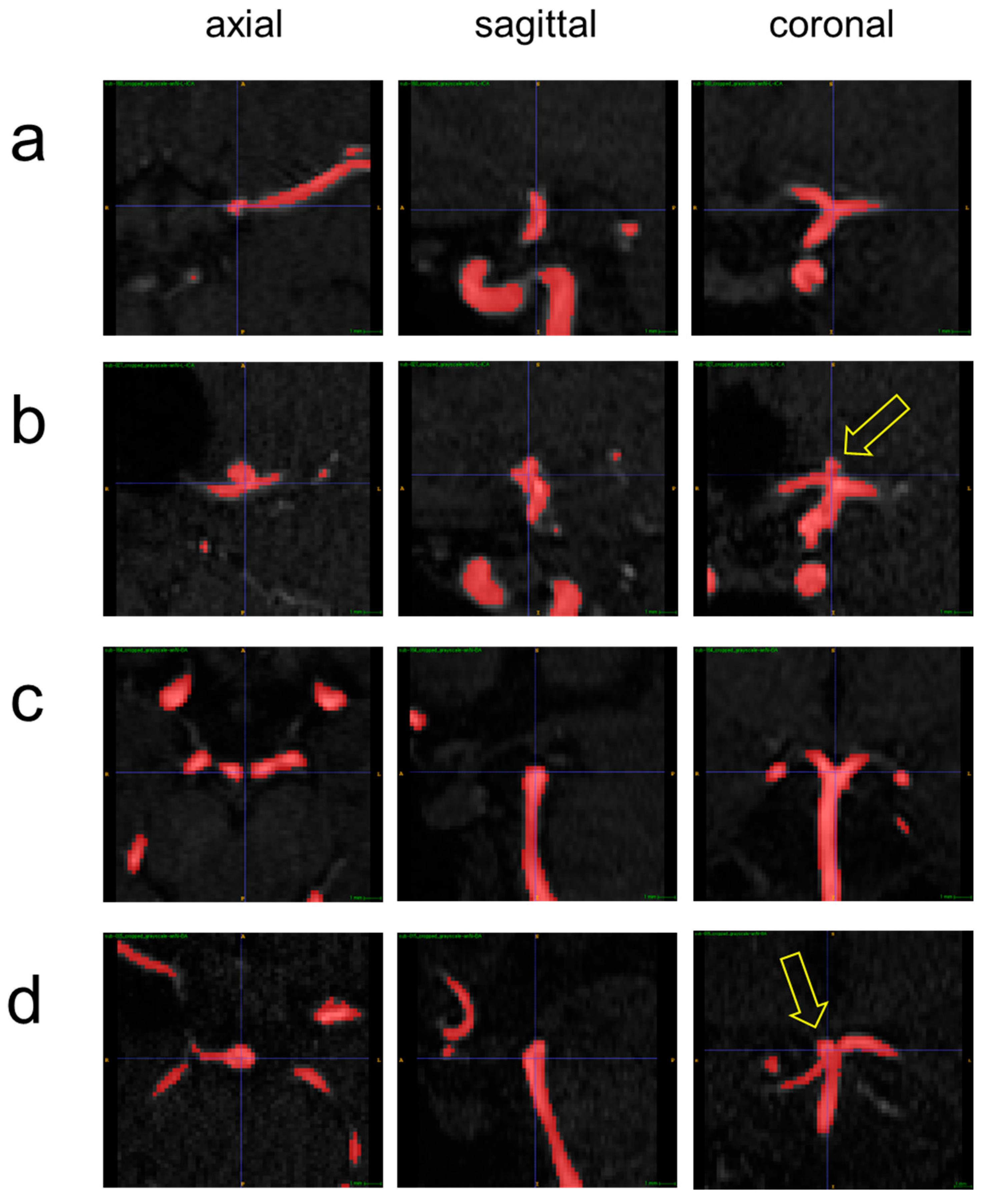
In addition, the 3D cropped gray-scale images and the 3D cropped segmented arterial masks were saved as .nii files. After loading the .nii files on the ITK-SNAP (version 3.8.0) software [23], we conducted a visual inspection of the images and their corresponding arterial masks as well as the 3D rendering of the arteries, and ensured that the bifurcations were centered around the 3D patches. Figure 3 shows representative examples of three orthogonal slices (i.e., axial, sagittal, coronal) in non-aneurysm and aneurysm 3D patches of certain bifurcation regions of interest observed from the ITK-SNAP user interface tool.

2.3. Model Development

Deep learning model development was performed using PyTorch (version 2.8.0) library [24]. The code for 3D CNN model architectures was based on publicly available Python scripts at the website [25]. The data were split into training, validation, and test groups while ensuring that any subject’s data were confined to only one of the three groups. The data split was performed after mixing the subjects from the two datasets. The training/validation/test splitting was performed with the ratio of 3:1:1 subject-wise. When there was no use of data augmentation, the numbers of 3D patches for the training, validation, and test were 336 (aneurysm = 74, non-aneurysm = 262), 129 (aneurysm = 19, non-aneurysm = 110), and 120 (aneurysm = 23, non-aneurysm = 97), respectively.
The 3D patches of the 64 × 64 × 64 dimensions were used as input to 3D CNN classifiers. We compared eight available 3D CNN architectures, including ResNet [26], DenseNet [27], EfficientNet [28], MobileNet [29], and ShuffleNet [30], which are available in [25]. The output was a probability score of being the ‘aneurysm’ class.
We utilized data augmentation, where transformed data are used for the training. Four data augmentation schemes were used: (1) original data only, (2) original data and flip along x, y, and z, (3) original data and translation along x, y, and z, (4) original data, flip along x, y, and z, and translation along x, y, and z. Table 2 shows the numbers of 3D patches for each data augmentation scheme. Data augmentation was applied to both aneurysm and non-aneurysm samples, while preserving class imbalance. For transformation, we utilized the TorchIO library, which provides multiple intensity and spatial transforms for data augmentation and preprocessing in 3D medical images [31]. For data augmentation, we used RandomFlip and RandomAffine classes available in TorchIO. The range for the translation was from −3 to 3. We compared the performance between without and with augmentation. The (x, y, z) translation appears as an appropriate choice for data augmentation, because, in a scenario of automatic bifurcation localization, the localization of the bifurcation point could be subject to errors [10]. Moreover, either L-R, S-I, or A-P flips of the 3D patches would be feasible in unseen test data, and hence we chose RandomFlip for data augmentation.
For hyperparameter tuning, training and validation were performed up to 30 epochs with learning rates of 0.001, 0.0005, and 0.0001 in eight 3D CNN models. During training, batch size was set to 32. For a given learning rate, the model weight parameters were saved at every epoch. During validation, a model to be used on test data was selected based on early stopping. After selection of the learning rate as a result of hyperparameter tuning, three 3D CNN models producing the highest precision recall area under the curve (PR-AUC) were chosen for further training and validation, which were performed up to 50 epochs with early stopping as regularization. The threshold corresponding to the maximum Youden index (i.e., sensitivity + specificity − 1) was also saved in order to be used to calculate the metrics of accuracy, precision, recall, and F1-score for the test data. Since data were imbalanced between the aneurysm and non-aneurysm classes, we specified weights such that the minor ‘aneurysm’ class was assigned to high weight value, and the major ‘non-aneurysm’ class was assigned to low weight value when using the PyTorch’s CrossEntropyLoss function as the loss function.

2.4. Evaluation

The deep 3D CNN models were trained and tested on a Windows PC equipped with 14th Gen Intel® CoreTM i9-14900, 32 GB RAM, and NVIDIA RTX A4000 GPU (16 GB memory). We used the Scikit-learn library [32] to calculate the metrics of PR-AUC, ROC-AUC, accuracy, precision, recall, and F1-score. The evaluation was performed on unseen test data.
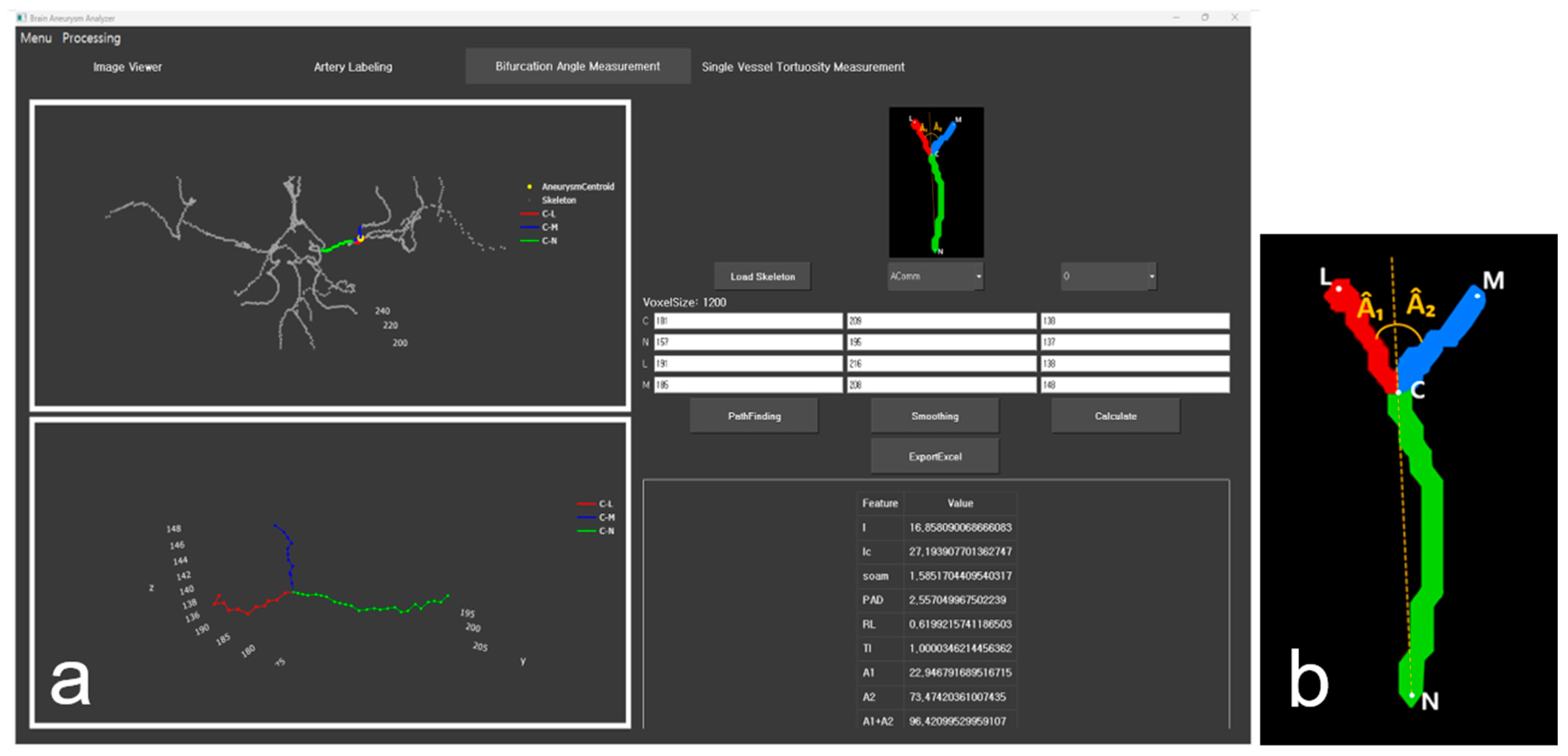
We measured vascular geometry using our custom graphical user interface software (Figure 4a) [33], which was implemented using PyQt library in Python [34]. The arterial centerlines after skeletonization were converted to graph structures using the Skan library [35]. To compute tortuosity metrics such as sum of angle metric (SOAM), we performed spline interpolation for smoothing the centerlines [19]. As shown in Figure 4b, we also computed the angle between the two daughter branches, the angle between the extension line of the parent artery and the one daughter branch, and the angle between the extension line of the parent artery and the other daughter branch.
We dichotomized test samples into high-probability score and low-probability score groups based on the probability score threshold of 0.5. Statistical analysis was performed using Python. An unpaired t-test was performed to compare arterial geometric measurements between high- and low-prediction score groups. The Shapiro–Wilk normality test was used for the high- and low-prediction score groups. A p-value < 0.05 was considered as statistically significant.

3. Results

Table 3 shows the prediction performance of the eight deep 3D CNN models when performing a tuning of the learning rate as a hyperparameter. The maximum number of epochs was set to 30. Data augmentation was not considered. Twenty seed numbers were used to generate twenty different combinations of train/validation/test data sample splits. Overall, the ResNetV2_18 model produced the highest mean PR-AUC score. The second and third best performing models were the ShuffleNet and ResNetV2_50 models, respectively. All three models produced their highest PR-AUC values when the learning rate was set to 0.001. We considered these three models to compare the prediction performances with respect to data augmentation methods.
For the learning rate of 0.001, which produced the highest PR-AUC scores, we trained the three best-performing models (i.e., ResNetV2_18, ResNetV2_50, ShuffleNet) with four different augmentation methods. Twenty seed numbers were used to generate twenty different combinations of training/validation/test data splits. The total training time was 8 h and 9 min, comprising three 3D CNN models trained with four different data augmentation schemes, each repeated across twenty random seeds. Table 4 compares the average per epoch time in training. The ‘no augment’ scheme took the shortest average per epoch time in each of the three models, while the ‘flip and translation’ scheme took the longest average per epoch time. The ShuffleNet models known as a lightweight neural network architecture were the fastest in training with the average per epoch time ranging from 1.09 to 3.82 s.
Table 5 compares three different network models’ prediction performance in test data. Data augmentation tended to improve prediction performances in all three models. In ResNetV2_18, data augmentation with translation only achieved the highest mean values in all metrics except for precision. In ResNetV2_50, data augmentation with flip and translation achieved the highest mean values in all metrics except for recall. In ShuffleNet, data augmentation with translation only achieved the highest mean values in all metrics except for accuracy. Overall, ResNetV2_18 with translation only produced the highest mean scores in accuracy, recall, F1-score, ROC-AUC, and PR-AUC metrics. The overall mean inference time was 0.0037 s per sample.
Table 6 shows the statistical significance test results in pairs of the three best-performing models in terms of PR-AUC on the test dataset. A paired t-test was performed to evaluate statistical significance. All three comparisons resulted in p-values > 0.05, indicating that there are no statistically significant differences in PR-AUCs in any pair of the three models.
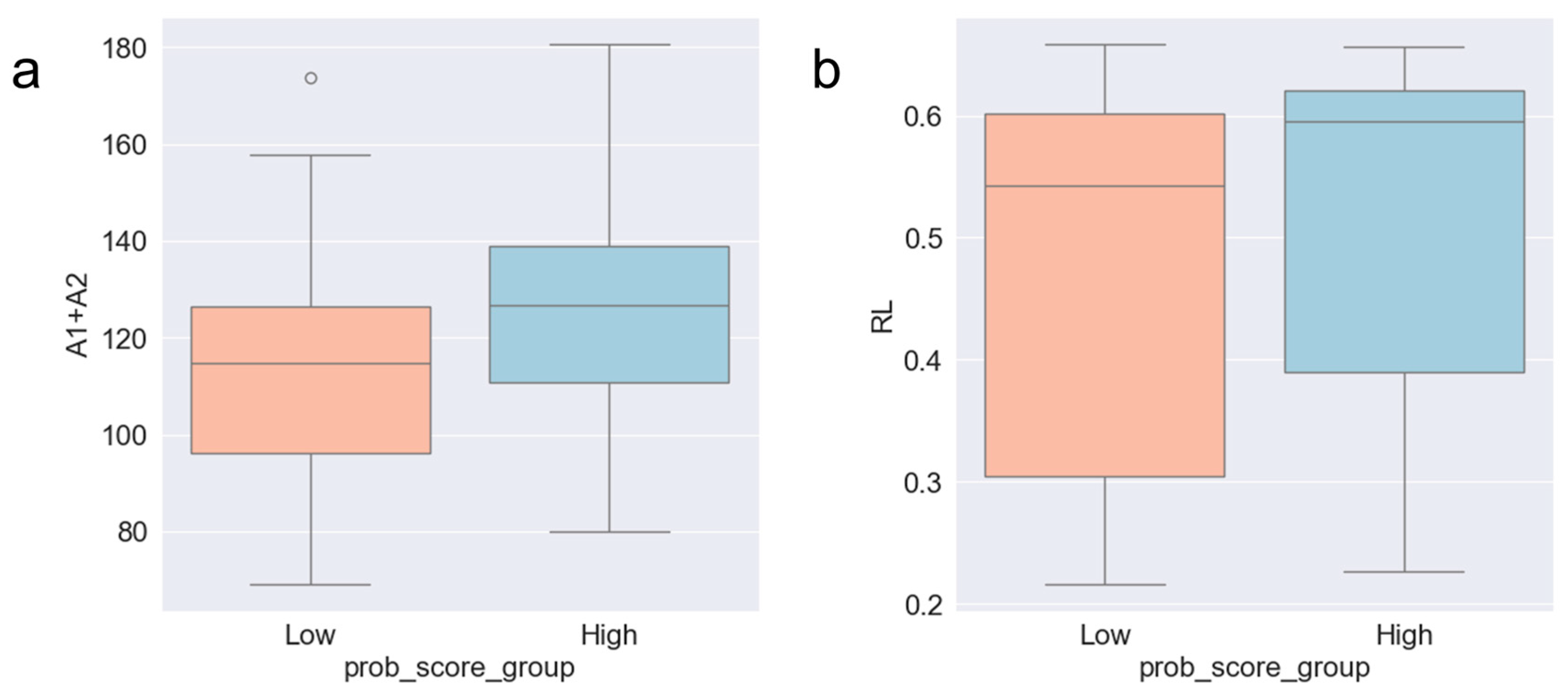
Figure 5 shows the dichotomization analysis results. The bifurcation angle sum (i.e., A1 + A2) values in the low- and high-probability score groups followed normal distributions based on the Shapiro–Wilk test, with the p-values 0.26 for the low-score group and 0.73 for the high-score group. For the bifurcation angle sum feature (i.e., A1 + A2) in Figure 5a, there was a statistically significant difference (t = −2.280, p-value = 0.025) between the low-score and the high-score groups. The relative length (i.e., RL) values in the low- and high-probability score groups did not follow normal distributions based on the Shapiro–Wilk test, with the p-values < 0.0001 for both the low- and high-score groups. For the relative length feature (i.e., RL) in Figure 5b, there was no statistical significance (t = −1.595, p-value = 0.114) between the low-score and the high-score groups. Although not shown in Figure 5, we performed the Shapiro–Wilk test on the sum-of-angles values of the low- and high-probability score groups with the p-values < 0.0001 for both the low- and high-score groups. We also performed a statistical significance test for the SOAM values and found no statistical significance (t = 1.462, p-value = 0.147) between the low-score and the high-score groups.

4. Discussion

We proposed the application of 3D CNN-based classifier models to predict the presence or absence of a cerebral aneurysm in small 3D patches of the 3D TOF MRA data. Several 3D CNN architectures were compared with different learning rates and data augmentation methods. The label annotations relied on the aneurysm lesion masks provided by the two public datasets. The regions of interest for the extraction of 3D patches were the bifurcations of the cerebral arteries near the CoW, where most of the cerebral aneurysm lesions occur. In addition, we compared the arteries’ bifurcation angle measurements with the deep learning models’ aneurysm predictions and found a difference in the angle sum measurement between the high and the low deep learning prediction groups.
In this study, we focused on the aneurysm predictions on the 3D patches of the bifurcation regions of interest as we were concerned with the comparison of geometric measurements in the bifurcations with the deep learning-based predictions. There were other types of aneurysms not located in the bifurcations in the CoW. In particular, it was noted that the LUH dataset had numerous aneurysm cases outside the CoW.
This study dealt with a scenario of class imbalance where the number of the non-aneurysm data was approximately four to five times as many as the number of the aneurysm data. To alleviate the class imbalance issue in the model development, we used the class-weighted loss function to provide a larger penalty on the minority class. Alternatively, one can consider using over-sampling on the minority class and achieving the balance between the two classes. This over-sampling approach appears challenging because the generation of 3D patches with an aneurysm is not straightforward to achieve. It is noted that recent studies demonstrate data augmentation using a synthetic vascular model, which can generate the vascular tree with aneurysms of any shape and size [36]. This would help improve the detection performance.
The deep learning-based aneurysm prediction on the 3D patches with large aneurysms is an easy task because of the noticeable appearance of the large aneurysm, but the presence of the large aneurysm makes it difficult to focus on the vascular geometry, which is essential for feature extraction in deep CNN. The patches in the contralateral hemisphere in the brain are free from the aneurysms, and thus they may be useful for training if the symmetrical configuration of both arteries is assumed. For example, the L-ICA and R-ICA can be assumed to have very similar vascular arrangements in a subject. Alternatively, if the aneurysm itself hinders the learning of the vascular geometry in deep CNN training, one may consider using advanced image processing techniques, such as image inpainting, with an aim to remove the aneurysm lesion. The deep learning-based image inpainting is a very active area of research encompassing medical imaging fields of dental artifact removal in magnetic resonance imaging [37].
In the measurement of the bifurcation angle or arterial tortuosity, some 3D patch data were discarded due to the thin and small size of the arteries. The extraction of the centerlines relied on voxel-based processing, which resulted in missing centerlines, especially in the PComm arteries in our study. Recent topology-based centerline extraction has the potential to increase the number of valid arteries used to calculate the geometry of the arteries [38].
We utilized our custom software tool for geometric analysis of the arteries in the bifurcations. It was noted that in some cases of having very large aneurysms, it was difficult to automatically locate the bifurcation center point due to the big size of the aneurysm. Since a big aneurysm is easily detectable, it was not considered for the evaluation of the relationship between the AI prediction scores and the geometric measurements in the bifurcation regions of interest.
Our study has limitations. First, we did not perform sensitivity analysis by masking aneurysm sacs or using contralateral bifurcations. Considering contralateral bifurcations would be reasonable with the assumption of symmetry in the bifurcations. Such sensitivity analysis may help train CNN models that predict aneurysm risks solely based on pre-aneurysmal arterial geometry. Second, we only included data from patients with aneurysms located at CoW bifurcations. This excluded a large portion of patient data with either aneurysms outside the CoW or aneurysms located in the middle of arteries. Third, we did not perform inter-rater reliability analysis for the bifurcation selection process. In the case of excluding large aneurysm datasets, the evaluation of inter-rater agreement would strengthen geometry-based analysis studies. Fourth, we did not investigate saliency analyses of the CNN architectures, which would enhance the explainability of the CNN models.

5. Conclusions

We have demonstrated a deep learning-based approach to the prediction of aneurysmal risks in the bifurcation regions of interest. The method focused on obtaining training data in small 3D patches around the bifurcation regions of interest in intracranial TOF MRA images. ResNetV2_18 with translation as data augmentation achieved the highest mean PR-AUC and ROC-AUC scores, but the model’s performance was not statistically significant in terms of PR-AUC when compared to the second best model. The group with high AI-predicted aneurysm probability scores demonstrated larger angle sum measurements at the bifurcations. This suggests that deep learning has the potential to screen bifurcations with high aneurysmal risks, without resorting to rigorous and time-consuming procedures of arterial geometry measurements.

Author Contributions

Conceptualization: Y.-C.K.; Data curation: Y.-C.K., J.-M.O., C.-U.Y., J.-W.K., H.L., and Y.L.; Formal analysis: J.-M.O., C.-U.Y., J.-W.K., H.L., and Y.-C.K.; Funding acquisition: Y.-C.K.; Investigation: Y.-C.K.; Methodology: Y.-C.K., J.-M.O., and C.-U.Y.; Project administration: Y.-C.K.; Resources: Y.-C.K.; Software: Y.-C.K., J.-M.O., and C.-U.Y.; Supervision: Y.-C.K.; Validation: C.-U.Y., J.-M.O., J.-W.K., and Y.L.; Visualization: J.-M.O., C.-U.Y.; Writing—original draft: Y.-C.K.; Writing—review and editing: Y.-C.K., C.-U.Y., Y.L., and J.-M.O. All authors have read and agreed to the published version of the manuscript.

Funding

This research was supported by the Regional Innovation System & Education (RISE) program through the Gangwon RISE Center, funded by the Ministry of Education (MOE) and the Gangwon State (G.S.), Republic of Korea (2025-RISE-10-006).

Data Availability Statement

The data supporting the conclusions of this article will be made available by the authors on request.

Conflicts of Interest

The authors declare no conflict of interest.

References

  1. Hackenberg, K.A.M.; Hanggi, D.; Etminan, N. Unruptured Intracranial Aneurysms. Stroke 2018, 49, 2268–2275. [Google Scholar] [CrossRef]
  2. Chalouhi, N.; Hoh, B.L.; Hasan, D. Review of cerebral aneurysm formation, growth, and rupture. Stroke 2013, 44, 3613–3622. [Google Scholar] [CrossRef]
  3. Song, M.; Wang, S.; Qian, Q.; Zhou, Y.; Luo, Y.; Gong, X. Intracranial aneurysm CTA images and 3D models dataset with clinical morphological and hemodynamic data. Sci. Data 2024, 11, 1213. [Google Scholar] [CrossRef] [PubMed]
  4. Jeon, T.Y.; Jeon, P.; Kim, K.H. Prevalence of unruptured intracranial aneurysm on MR angiography. Korean J. Radiol. 2011, 12, 547–553. [Google Scholar] [CrossRef]
  5. Toth, G.; Cerejo, R. Intracranial aneurysms: Review of current science and management. Vasc. Med. 2018, 23, 276–288. [Google Scholar] [CrossRef]
  6. Claux, F.; Baudouin, M.; Bogey, C.; Rouchaud, A. Dense, deep learning-based intracranial aneurysm detection on TOF MRI using two-stage regularized U-Net. J. Neuroradiol. 2023, 50, 9–15. [Google Scholar] [CrossRef]
  7. Heit, J.J.; Honce, J.M.; Yedavalli, V.S.; Baccin, C.E.; Tatit, R.T.; Copeland, K.; Timpone, V.M. RAPID Aneurysm: Artificial intelligence for unruptured cerebral aneurysm detection on CT angiography. J. Stroke Cerebrovasc. Dis. 2022, 31, 106690. [Google Scholar] [CrossRef]
  8. Zhou, Z.; Jin, Y.; Ye, H.; Zhang, X.; Liu, J.; Zhang, W. Classification, detection, and segmentation performance of image-based AI in intracranial aneurysm: A systematic review. BMC Med. Imaging 2024, 24, 164. [Google Scholar] [CrossRef]
  9. Anima, V.; Nair, M.S. On the automated unruptured intracranial aneurysm segmentation from tof-mra using deep learning techniques. IEEE Access 2024, 12, 53112–53125. [Google Scholar] [CrossRef]
  10. Nader, R.; Bourcier, R.; Autrusseau, F. Using deep learning for an automatic detection and classification of the vascular bifurcations along the Circle of Willis. Med. Image Anal. 2023, 89, 102919. [Google Scholar] [CrossRef]
  11. Bor, A.S.; Velthuis, B.K.; Majoie, C.B.; Rinkel, G.J. Configuration of intracranial arteries and development of aneurysms: A follow-up study. Neurology 2008, 70, 700–705. [Google Scholar] [CrossRef] [PubMed]
  12. Zhang, X.J.; Gao, B.L.; Li, T.X.; Hao, W.L.; Wu, S.S.; Zhang, D.H. Association of Basilar Bifurcation Aneurysms with Age, Sex, and Bifurcation Geometry. Stroke 2018, 49, 1371–1376. [Google Scholar] [CrossRef] [PubMed]
  13. Baharoglu, M.I.; Lauric, A.; Safain, M.G.; Hippelheuser, J.; Wu, C.; Malek, A.M. Widening and high inclination of the middle cerebral artery bifurcation are associated with presence of aneurysms. Stroke 2014, 45, 2649–2655. [Google Scholar] [CrossRef] [PubMed]
  14. Dhar, S.; Tremmel, M.; Mocco, J.; Kim, M.; Yamamoto, J.; Siddiqui, A.H.; Hopkins, L.N.; Meng, H. Morphology parameters for intracranial aneurysm rupture risk assessment. Neurosurgery 2008, 63, 185–196; discussion 196–197. [Google Scholar] [CrossRef]
  15. Mocco, J.; Brown, R.D., Jr.; Torner, J.C.; Capuano, A.W.; Fargen, K.M.; Raghavan, M.L.; Piepgras, D.G.; Meissner, I.; Huston, J., III. International Study of Unruptured Intracranial Aneurysms, I. Aneurysm Morphology and Prediction of Rupture: An International Study of Unruptured Intracranial Aneurysms Analysis. Neurosurgery 2018, 82, 491–496. [Google Scholar] [CrossRef]
  16. Di Noto, T.; Marie, G.; Tourbier, S.; Aleman-Gomez, Y.; Esteban, O.; Saliou, G.; Cuadra, M.B.; Hagmann, P.; Richiardi, J. Towards Automated Brain Aneurysm Detection in TOF-MRA: Open Data, Weak Labels, and Anatomical Knowledge. Neuroinformatics 2023, 21, 21–34. [Google Scholar] [CrossRef]
  17. de Nys, C.M.; Liang, E.S.; Prior, M.; Woodruff, M.A.; Novak, J.I.; Murphy, A.R.; Li, Z.Y.; Winter, C.D.; Allenby, M.C. Time-of-Flight MRA of Intracranial Aneurysms with Interval Surveillance, Clinical Segmentation and Annotations. Sci. Data 2024, 11, 555. [Google Scholar] [CrossRef]
  18. Javed, A.; Kim, Y.C.; Khoo, M.C.; Ward, S.L.; Nayak, K.S. Dynamic 3-D MR Visualization and Detection of Upper Airway Obstruction During Sleep Using Region-Growing Segmentation. IEEE Trans. Biomed. Eng. 2016, 63, 431–437. [Google Scholar] [CrossRef]
  19. Yoon, H.S.; Oh, J.; Kim, Y.C. Assessing Machine Learning Models for Predicting Age with Intracranial Vessel Tortuosity and Thickness Information. Brain Sci. 2023, 13, 1512. [Google Scholar] [CrossRef]
  20. Van der Walt, S.; Schönberger, J.L.; Nunez-Iglesias, J.; Boulogne, F.; Warner, J.D.; Yager, N.; Gouillart, E.; Yu, T. scikit-image: Image processing in Python. PeerJ 2014, 2, e453. [Google Scholar] [CrossRef]
  21. Kim, S.O.; Kim, Y.C. Effects of Path-Finding Algorithms on the Labeling of the Centerlines of Circle of Willis Arteries. Tomography 2023, 9, 1423–1433. [Google Scholar] [CrossRef]
  22. Kim, S.O.; Kim, Y.C. An Improved Path-Finding Method for the Tracking of Centerlines of Tortuous Internal Carotid Arteries in MR Angiography. J. Imaging 2024, 10, 58. [Google Scholar] [CrossRef] [PubMed]
  23. Yushkevich, P.A.; Piven, J.; Hazlett, H.C.; Smith, R.G.; Ho, S.; Gee, J.C.; Gerig, G. User-guided 3D active contour segmentation of anatomical structures: Significantly improved efficiency and reliability. Neuroimage 2006, 31, 1116–1128. [Google Scholar] [CrossRef] [PubMed]
  24. Paszke, A.; Gross, S.; Massa, F.; Lerer, A.; Bradbury, J.; Chanan, G.; Killeen, T.; Lin, Z.; Gimelshein, N.; Antiga, L. Pytorch: An imperative style, high-performance deep learning library. In Proceedings of the 33rd International Conference on Neural Information Processing Systems, Vancouver, BC, Canada, 8–14 December 2019. [Google Scholar]
  25. 3D-CNN-PyTorch: PyTorch Implementation for 3dCNNs for Medical Images. Available online: https://github.com/xmuyzz/3D-CNN-PyTorch (accessed on 13 November 2025).
  26. He, K.; Zhang, X.; Ren, S.; Sun, J. Deep residual learning for image recognition. In Proceedings of the IEEE Conference on Computer Vision and Pattern Recognition, Las Vegas, NV, USA, 26 June–1 July 2016; pp. 770–778. [Google Scholar]
  27. Huang, G.; Liu, Z.; Van Der Maaten, L.; Weinberger, K.Q. Densely connected convolutional networks. In Proceedings of the IEEE Conference on Computer Vision and Pattern Recognition, Honolulu, HI, USA, 21–26 July 2017; pp. 4700–4708. [Google Scholar]
  28. Tan, M.; Le, Q. Efficientnet: Rethinking model scaling for convolutional neural networks. In Proceedings of the International Conference on Machine Learning, Long Beach, CA, USA, 10–15 June 2019; pp. 6105–6114. [Google Scholar]
  29. Howard, A.G.; Zhu, M.; Chen, B.; Kalenichenko, D.; Wang, W.; Weyand, T.; Andreetto, M.; Adam, H. Mobilenets: Efficient convolutional neural networks for mobile vision applications. arXiv 2017, arXiv:1704.04861. [Google Scholar] [CrossRef]
  30. Zhang, X.; Zhou, X.; Lin, M.; Sun, J. Shufflenet: An extremely efficient convolutional neural network for mobile devices. In Proceedings of the IEEE Conference on Computer Vision and Pattern Recognition, Salt Lake City, UT, USA, 18–22 June 2018; pp. 6848–6856. [Google Scholar]
  31. Perez-Garcia, F.; Sparks, R.; Ourselin, S. TorchIO: A Python library for efficient loading, preprocessing, augmentation and patch-based sampling of medical images in deep learning. Comput. Methods Programs Biomed. 2021, 208, 106236. [Google Scholar] [CrossRef]
  32. Pedregosa, F.; Varoquaux, G.; Gramfort, A.; Michel, V.; Thirion, B.; Grisel, O.; Blondel, M.; Prettenhofer, P.; Weiss, R.; Dubourg, V. Scikit-learn: Machine learning in Python. J. Mach. Learn. Res. 2011, 12, 2825–2830. [Google Scholar]
  33. Oh, J.; Kim, Y.-C. Software design for quantitative analysis of geometric features of the vessels with cerebral aneurysms in MR angiography 3D images. J. Korean Inst. Next Gener. Comput. 2024, 20, 56–65. [Google Scholar]
  34. Summerfield, M. Rapid GUI Programming with Python and Qt: The Definitive Guide to PyQt Programming; Pearson Education: London, UK, 2007. [Google Scholar]
  35. Nunez-Iglesias, J.; Blanch, A.J.; Looker, O.; Dixon, M.W.; Tilley, L. A new Python library to analyse skeleton images confirms malaria parasite remodelling of the red blood cell membrane skeleton. PeerJ 2018, 6, e4312. [Google Scholar] [CrossRef]
  36. Nader, R.; Autrusseau, F.; L’Allinec, V.; Bourcier, R. Building a Synthetic Vascular Model: Evaluation in an Intracranial Aneurysms Detection Scenario. IEEE Trans. Med. Imaging 2024, 44, 1347–1358. [Google Scholar] [CrossRef]
  37. Xie, K.; Gao, L.; Lu, Z.; Li, C.; Xi, Q.; Zhang, F.; Sun, J.; Lin, T.; Sui, J.; Ni, X. Inpainting the metal artifact region in MRI images by using generative adversarial networks with gated convolution. Med. Phys. 2022, 49, 6424–6438. [Google Scholar] [CrossRef]
  38. Alblas, D.; Vos, I.N.; Lipplaa, M.M.; Brune, C.; van der Schaaf, I.C.; Velthuis, M.R.E.; Velthuis, B.K.; Kuijf, H.J.; Ruigrok, Y.M.; Wolterink, J.M. Deep-learning-based extraction of circle of Willis topology with anatomical priors. Sci. Rep. 2024, 14, 31630. [Google Scholar] [CrossRef]
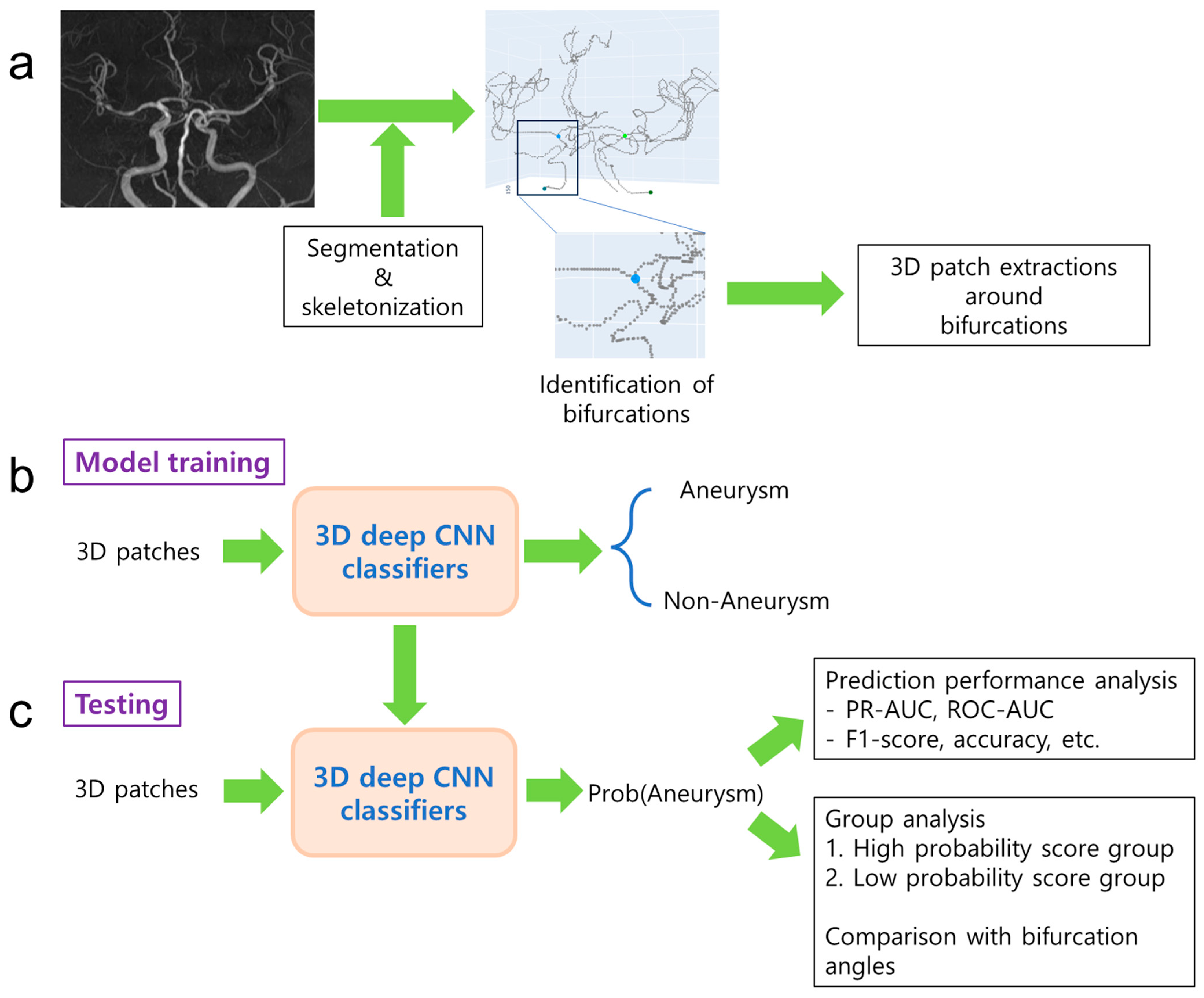
Figure 1. Flowchart of our study. (a) Three-dimensional patch extraction. (b). Model training. (c). Model testing.
Applsci 15 13004 g001
Figure 2. Illustration of bifurcations and their corresponding names. The colors represent arterial centerlines in the circle of Willis.
Applsci 15 13004 g002
Figure 3. Mid-axial, mid-sagittal, and mid-coronal slices of the 3D patches with the dimensions of 64 × 64 × 64. The bifurcations are located at the centers of the 3D patches. (a). Subject A’s L-ICA bifurcation region of interest, with no aneurysm. (b). Subject B’s L-ICA bifurcation region of interest, with aneurysm indicated by the yellow arrow. (c). Subject C’s BA bifurcation region of interest, with no aneurysm. (d). Subject D’s BA bifurcation region of interest, with aneurysm indicated by the yellow arrow.
Applsci 15 13004 g003
Figure 4. Measurements of arterial geometry in the bifurcation region of interest. (a) Our custom graphical user interface tool used for the evaluation of arterial tortuosity and angles between the parent artery and the daughter branches. (b) A zoomed-in illustration of the parent artery (C-N) and the two daughter branches (C-L) and (C-M).
Applsci 15 13004 g004
Figure 5. Comparisons between high-probability score and low-probability score groups. (a) Box plot showing A1 + A2 angle differences in groups. (b) Box plot showing relative length (RL) differences in groups.
Applsci 15 13004 g005
Table 1. The numbers of subjects and patches for the two datasets in training, validation, and test.
DatasetLabel TypeThe Number of SubjectsThe Number of 3D Patches
LUHAneurysm5859
Non-aneurysm100469
RBWHAneurysm4657
Total 204585
Table 2. The numbers of 3D patches for different schemes of data augmentation in training data.
Augmentation MethodThe Number of Training Samples
(1) No augmentation336
(2) Augmentation using flip672
(3) Augmentation using translation672
(4) Augmentation using flip and translation1344
Table 3. Tuning of learning rate on eight CNN models when augmentation was not used. The bolds indicate the highest three mean (standard deviation) values among all the models considered.
Learning RateMetricModel
DenseNet121DenseNet169EfficientNetMobileNetResNetV2_18ResNetV2_34ResNetV2_50ShuffleNet
0.001PR-AUC0.306 (0.123)0.311 (0.060)0.216 (0.051)0.250 (0.070)0.393 (0.106)0.347 (0.085)0.357 (0.095)0.373 (0.114)
0.0005PR-AUC0.332 (0.108)0.315 (0.092)0.217 (0.058)0.258 (0.078)0.351 (0.117)0.331 (0.093)0.349 (0.096)0.347 (0.119)
0.0001PR-AUC0.334 (0.107)0.285 (0.129)0.207 (0.045)0.258 (0.098)0.270 (0.084)0.242 (0.068)0.310 (0.104)0.313 (0.087)
Table 4. Comparison of average per epoch time in training.
ModelAugmentation
Method
Average per Epoch Time in Training (Seconds)
ResNetV2_18No augment3.48
Flip5.16
Translation5.17
Flip and translation8.62
ResNetV2_50No augment5.10
Flip8.05
Translation8.06
Flip and translation13.87
ShuffleNetNo augment1.09
Flip2.00
Translation2.01
Flip and translation3.82
Table 5. Performance evaluation on test data for different schemes of data augmentation. The values are shown in mean (standard deviation).
ModelAugmentation
Method
AccuracyPrecisionRecallF1-scoreROC-AUCPR-AUC
ResNetV2_18No augment0.682 (0.105)0.338 (0.094)0.629 (0.180)0.425 (0.097)0.695 (0.072)0.411 (0.106)
Flip 0.693 (0.115)0.363 (0.137)0.575 (0.161)0.417 (0.083)0.708 (0.084)0.451 (0.097)
Translation 0.698 (0.099)0.364 (0.118)0.655 (0.122)0.454 (0.098)0.735 (0.076)0.472 (0.116)
Flip and translation 0.656 (0.154)0.365 (0.200)0.584 (0.185)0.400 (0.119)0.705 (0.085)0.470 (0.139)
ResNetV2_50No augment0.642 (0.127)0.296 (0.112)0.511 (0.157)0.352 (0.083)0.629 (0.094)0.349 (0.109)
Flip0.629 (0.117)0.292 (0.089)0.595 (0.160)0.376 (0.082)0.667 (0.072)0.386 (0.090)
Translation0.663 (0.098)0.316 (0.142)0.497 (0.180)0.348 (0.098)0.666 (0.065)0.395 (0.088)
Flip and translation0.664 (0.103)0.326 (0.119)0.573 (0.171)0.389 (0.080)0.697 (0.072)0.427 (0.096)
ShuffleNetNo augment0.608 (0.149)0.262 (0.125)0.574 (0.232)0.344 (0.139)0.639 (0.131)0.382 (0.139)
Flip0.619 (0.125)0.270 (0.092)0.528 (0.181)0.341 (0.097)0.626 (0.104)0.355 (0.099)
Translation0.658 (0.133)0.314 (0.105)0.604 (0.205)0.396 (0.125)0.692 (0.101)0.430 (0.140)
Flip and translation0.663 (0.101)0.307 (0.112)0.542 (0.154)0.375 (0.107)0.674 (0.079)0.429 (0.109)
Table 6. Statistical significance test results in terms of PR-AUC among three models.
Model AModel BModel A
PR-AUC
Model B
PR-AUC
p-Value95% Confidence Interval
ResNetV2_18
(translation)
ResNetV2_50
(flip and translation)
0.472 (0.116)0.427 (0.096)0.102[−0.010, 0.100]
ResNetV2_50
(flip and translation)
ShuffleNet
(translation)
0.427 (0.096)0.430 (0.140)0.930[−0.064, 0.059]
ShuffleNet
(translation)
ResNetV2_18
(translation)
0.430 (0.140)0.472 (0.116)0.194[−0.023, 0.108]
Disclaimer/Publisher’s Note: The statements, opinions and data contained in all publications are solely those of the individual author(s) and contributor(s) and not of MDPI and/or the editor(s). MDPI and/or the editor(s) disclaim responsibility for any injury to people or property resulting from any ideas, methods, instructions or products referred to in the content.