Research on Energy Management Strategy for Range-Extended Electric Vehicles Based on Eco-Driving Speed

Abstract

To achieve the optimal energy allocation between the auxiliary power unit (APU) and battery of connected automated range-extended electric vehicle (CAR-EEV), the hierarchical eco-driving control with dynamic game energy management were investigated and the optimization design of APU working mode was carried out from a multi-objective perspective. Initially, the acceleration and speed of the host vehicle were adjusted in real time, based on the driving status of the preceding vehicle, and the ecological driving speed was obtained in the adaptive car-following eco-driving mode. The dynamic game energy management strategy was proposed, leveraging the real-time interactive information between the vehicle and the traffic environment, and intelligently allocating and scheduling the energy flow within the powertrain. Dynamic game optimization was adopted to achieve dynamic decision-making and control optimization on whether to switch the APU operating speed or not. The multi-objective optimization analyses are carried out based on the weight coefficient matrix. The hierarchical dynamic game energy management strategy based on eco-driving speed (HDGEMS) is implemented through dynamic games and exhibits excellent performance. This strategy enables dynamic adjustment of power distribution between the APU and the battery, thereby allowing the APU to operate efficiently under optimal operating conditions. Meanwhile, it effectively reduces secondary charging losses and the dynamic switching time of the APU, and ultimately achieves energy optimization. Eventually, the results of simulation and experimental thoroughly indicated that economy improvement, emission reduction, and battery life enhancement of CAR-EEV were effectively kept in balance under the control of the proposed HDGEMS with intelligent optimization mode. New research ideas and technical directions are provided for the field of EMS, which is expected to promote technological progress in the industry.

1. Introduction

Connected automated range-extended electric vehicles (CAR-EEVs) equipped with intelligent information systems have introduced complexities in their energy management strategies (EMSs) [1]. To address these challenges, extensive research is needed to develop a robust EMS capable of effectively managing multiple energy sources within the hybrid system for reliable power distribution. For the hierarchical eco-driving control, the adaptive car-following eco-driving strategy is an intelligent driving control approach, aiming to enhance driving safety and reduce energy consumption. The dynamic game energy management strategy is a more advanced energy scheduling method that utilizes the real-time interaction information between the vehicle and the traffic environment to intelligently allocate and schedule the energy flow of the power system [2]. For CAR-EEVs, the design of the APU operating mode and the multi-objective optimization (MOO) are the keys to achieving energy savings and emission reductions [3]. Therefore, through the optimized design of the APU operating mode/area, the influence of different operating modes of the APU system on the energy consumption, emissions, and battery health is studied from a multi-objective perspective, which is important for implementing the optimal energy distribution and realizing the comprehensive control effect of robust control in the multi-source V2X information environment [4].

1.1. Review of Literature

The CAR-EEV’s unique configurations with mechanical decoupling, flexible oil–electric distribution, and intelligent information system on board requires designing an optimal EMS for APU mode with V2X multi-source information [5]. APU operating more at the optimal point/area and minimizing rotational speed fluctuations can achieve optimal energy distribution via CAR-EEV advantages, enhancing overall control performance in energy consumption, emissions, and battery health. However, optimized parameters may only match specific driving cycle conditions and possess limited generalization ability [6,7].

In the eco-driving strategy, the fuel economy of CAR-EEV correlates closely with speed distribution as it directly impacts total energy consumption. The latest research shows that combining eco-driving and speed planning can effectively reduce energy consumption [8]. Deep learning-based driving behavior prediction technology has demonstrated strong potential, with driver habits accurately captured to optimize strategies; meanwhile, breakthroughs have been achieved in advanced battery management systems in improving the accuracy of battery life prediction, providing a more reliable basis for energy management. An eco-driving-based dynamic speed planning algorithm was proposed which can quickly control the speed within the speed limit range and enable the car to obtain relatively low energy consumption [9]. In urban areas with continuous signalized intersections, computing a reference speed curve to avoid worthless idling enhances energy savings. Model predictive control (MPC) was used to calculate reference speed in dense traffic, in which vehicles are forced to follow the car in front [10]. CAR-EEV fuel-saving performance hinges on speed distribution, making reasonable speed planning essential for the overall eco-driving strategy. In the domain of eco-driving strategies, hierarchical strategies are relatively common. The hierarchical optimization framework decomposed the hybrid optimization problem into discrete and continuous ones. A multi-step optimal-based decision-making architecture is developed to compute optimal acceleration profiles for adaptive cruise control in V2X-enabled environments [11]. Although studies on eco-driving and driving styles have been conducted, relatively little research exists regarding the relationship between drivers’ driving styles and vehicle eco-driving optimization, especially for eco-driving speeds on long-distance urban roads [12]. From the above analysis, it is evident that in the eco-driving strategy, the fuel economy of CAR-EEV is closely associated with speed distribution. The speed distribution, which determines the total energy demand, is a crucial factor in the strategy [13]. Moreover, as environmental information and driving styles impact the eco-driving strategy, reasonable speed planning should be incorporated.

Many studies focus on macroscopic traffic management and control, using dynamic game algorithms for energy management strategies and multi-objective optimization to enhance vehicle performance on complex roads. As vehicle networking and traffic info interact, establishing a V2X-based game decision method to solve control conflicts is a focus [14]. Game theory has been widely applied in the fields of intelligent transportation and vehicle control to investigate interactions among multiple intelligent agents [15]. In CAR-EEV energy management research, it is extensively applied to travel characteristics, route selection, power distribution, and mode switching. Game theory excels in explaining small spatiotemporal-scale–agent interactions, culminating in more studies in the CAR-EEV field. Fuzzy Markov chains in a game model predictive controller was introduced to predicted candidate vehicle motion [16]. Moreover, the optimization of EMS performance is a typical MOO problem, requiring independent and balanced results [17,18,19]. With the interaction of connected vehicles and traffic environment information, establishing a V2X-based game decision-making method to solve multi-objective control conflicts has become a research hotspot. The proposed EMS utilizes the CAR-EEV configuration to attain optimal energy distribution (minimizing large-span dynamic fluctuations in rotational speed and maximizing operation at the optimal point/area). Besides minimizing system energy consumption and emissions, extending battery life is another optimization goal. Because previous empirical or semi-empirical battery life models were limited to specific business systems and lacked transferability, most battery anti-aging EMSs with discrete solution processes are difficult to implement in vehicle control. A clear SoC reference trajectory is essential for planning battery power distribution to approach the global optimal [20].

Despite the numerous existing studies on eco-driving, driving styles, and energy management strategies, deficiencies in current research still persist. A hierarchical dynamic game energy-management strategy based on eco-driving speed (HDGEMS, EMS_he-dg) was investigated and the optimization design of the APU working mode was carried out from a multi-objective perspective, as proposed. At the upper level, environmental and driver factors directly influence driver behavior and decision-making, contributing to the inability to ensure the accuracy and safety of the eco-driving strategy. Thus, driver behavior characteristics are integrated into the car-following model from environmental and personal aspects, to fulfill the speed planning task. Considering the fuzziness of the reinforcement learning–reward function, imitation learning is adopted as the framework of the car-following model to imitate expert strategies for eco-driving optimization. At the lower level, the achievement of the APU multi-point working mode with dynamic game is focused. This method integrates imitation learning and dynamic game, with the expectation of significantly improving vehicle performance under complex road conditions.

1.2. Motivation and Innovation

In this paper, a dynamic game optimization method based on V2X information is proposed. Promisingly, the proposed EMS_he-dg with dynamic game optimization exhibited a significant multi-objective performance comprehensive balancing ability. The main contributions of this paper are highlighted in the following points. (1) Considering the impact of environmental and driver factors on the accuracy and safety of ecological driving strategies, driver behavior characteristics are integrated into the following model from both environmental and personal perspectives to complete the speed planning task of ecological driving strategies. (2) The APU multi-point working mode with dynamic game is designed and a dynamic game method with future driving prediction is used for APU operating speed-switching working, which is an intelligent decision-making mode that considers V2X information to achieve real-time driving feature identification and quantitative information. (3) A general framework of MOO is proposed for EMS_he-dg, with optimization of battery charge/discharge planning and APU working mode meeingt the MOO requirements of energy conservation, emission reduction, and battery lifespan enhancement. Compared with existing methods, the profit structure of the proposed HDGEMS game model in this study not only takes into account the economic benefits of energy allocation, but also innovatively integrates riding comfort indicators, making energy allocation decisions more aligned with actual driving needs, thereby providing a more accurate basis for power distribution between the APU and the battery and further optimizing energy allocation effects; additionally, the practical scope of imitation learning has been effectively expanded in this study, and by introducing richer historical driving data and real-time feedback information, the model can better adapt to different driving scenarios, achieving improved performance in energy conservation and emission reduction while battery life has been better prolonged.

2. Materials and Methods

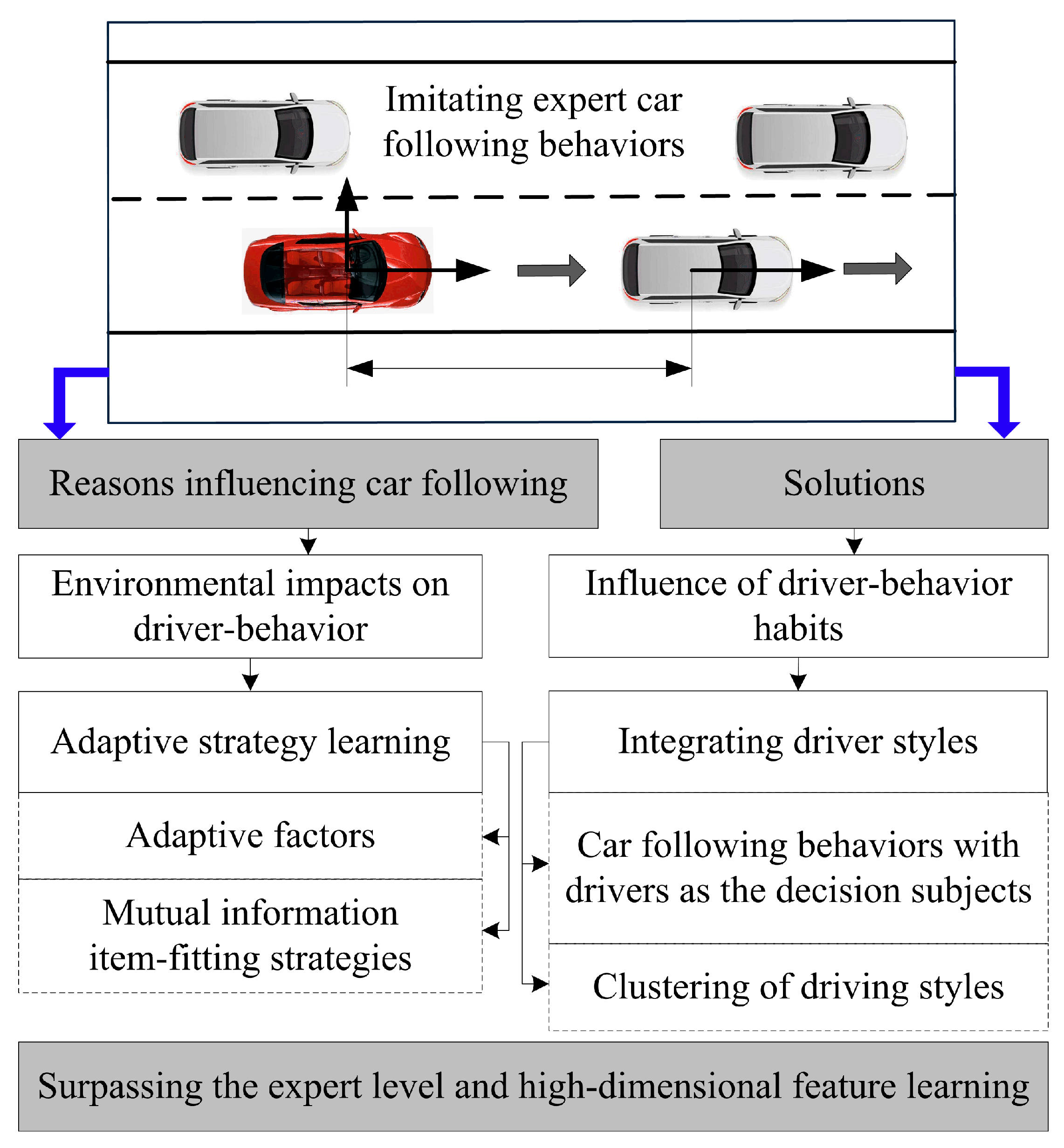
The factors that affect car following can be mainly divided into two aspects. The first is the influence of the environment itself on driver behavior, and the second is the inherent influence of individual driver behavior habits on the following strategy.

2.1. Theoretical Reference

For imitation learning methods, appropriate reward functions do not need to be manually set. Consequently, in complex and ill-defined environments, they outperform reinforcement learning methods. In actual tasks, there may be multiple intentions when drivers are following a vehicle; different drivers have different driving habits, such as aggressive and mild type, which will then lead to difficulties in choosing a reward function. To solve these problems, an adaptive learning strategy and imitation learning method was proposed, which fuses driving styles and enabled the conduction of further research and improvement. Figure 1 illustrates the algorithm flowchart of the adaptive car-following strategy based on imitation learning in this paper.

This section proposes the following model with an adaptive factor for the inherent phenomenon of environmental influence on driver behavior. The main idea is to construct a framework of a GAN network with adaptability based on the basic principle of the GAN network: that is, instead of estimating the reward function, directly learn the strategy of the following model. The formula is as shown in (1):

$$\left\{\begin{array}{l}\underset{\pi }{\min }\underset{D\in {(0,1)}^{s\times A}}{\max }{\mathbb{E}}_{\pi }[\log D(s,a)+{\mathbb{E}}_{\pi E}[\log (1-D(s,a)]-\lambda H(\pi )\\ {H(\pi )}_{\underset{¯}{\underset{¯}{△}}}{\mathbb{E}}_{\pi }[-\log (\left.\alpha \right|s)]\end{array}\right.$$

(1)

where π_E is the expert strategy; π is the strategy that needs to be learned and trained; D is used as a discriminator to distinguish state-action pairs; and H(π) represents causal entropy.

The adaptive strategy is model-free, but needs to be interactively trained with the environment. It treats the environment as a black box and is end-to-end differentiable. Due to internal potential variation factors such as expert level and preferences under different strategies, the generated trajectories will also have significant changes among different individuals. Even the same person when facing the same situation will make different decisions, as well, which leads to the generation of multiple different strategies. In this scenario, construct an expert strategy set: ${\pi }_E=\left\{{\pi }_E^0,{\pi }_E^1,\dots \right.\}$, and redefine the generation process $s_0\sim {\rho }_{0}c\sim p\left(c\right),\pi \sim p(\pi \mid c{)}_0{a}_t\sim \pi \left(a_t\mid s_t\right)$, $s_{t+1}\sim P\left(s_{t+1}\mid a_t,s_t\right)$ of expert trajectories ${\tau }_E$. In this process, an adaptive parameter c is defined, and $p\left(c\right)$ is the prior probability distribution of $c$. The goal of this algorithm is to recover the strategy $\pi (a\mid s,c)$ under the adaptive parameter $c$.

In order to make the adaptive factor more closely fit with the strategy, achieve a degree of interdependence, and make the adaptive factor and the strategy have greater correlation, mutual information is added to the optimization function.

$$I\left(c;\tau \right)=H(c)+{\mathbb{E}}_{c\sim p(c),a\sim \pi (\left.\cdot \right|s,c)}[\log p(\left.c\right|\tau )]$$

(2)

where $I\left(c;\tau \right)$ is the mutual information; H(c) is the entropy of the adaptive parameter c; p(c) is the prior probability distribution of the adaptive parameter c; π(·|s,c) is the probability distribution of actions given the state s and parameter c; τ is the expert trajectory; p(c|τ) is the posterior probability distribution of c given the expert trajectory τ; and $\mathbb{E}$ is the mathematical expectation.

Then add the adaptive factors to the optimization objective function to obtain

$$\underset{{\theta }_{-}\psi }{\mathrm{m}\mathrm{i}\mathrm{n}} \underset{\omega }{\mathrm{m}\mathrm{a}\mathrm{x}} {\mathbb{E}}_{{\pi }_{\theta }}\left[\log D_{\omega }\left(s,a\right)\right]+{\mathbb{E}}_{{\pi }_E}\left[\log \left(1-D_{\omega }\left(s,a\right)\right)\right]-{\lambda }_{1}I\left(c;\tau \right)-{\lambda }_{2}H\left({\pi }_{\theta }\right)$$

(3)

where $\theta \mathrm{a}\mathrm{n}\mathrm{d} \psi$ are the relevant parameters of the strategy to be learned; $\omega$ is the discriminator parameter; $D_{\omega }\left(s,a\right)$ is the discriminator function with parameter $\omega$; ${\pi }_{\theta }$ is the strategy to be learned; and ${\lambda }_1$ and ${\lambda }_2$ are the weight coefficients.

This can make the mixed trajectories generated by experts more clearly organized, but in the calculation process the posterior probability $p\left(c\right|\tau )$ is difficult to calculate. Here the Q value is directly used instead; that is

$$\left\{\begin{array}{l}{L}_1(\pi ,Q)\le I(c;\tau )\\ \underset{\theta \_\psi }{\min } \underset{\omega }{\max } {\mathbb{E}}_{\pi \theta }[\log D_{\omega }(s,a)]+\mathbb{E}[\log (1-D_{\omega }(s,a)]\\ -{\lambda }_1{L}_1(\pi ,Q)-{\lambda }_{2}H({\pi }_{\theta })\end{array}\right.$$

(4)

where L₁(π,Q) is a metric related to the policy π and the Q-value (since the posterior probability p(c|τ) is difficult to calculate, it is used to approximate the mutual information $I\left(c;\tau \right)$).

During vehicle driving, one should not only consider the influence of the driving environment on the model, but should also satisfy the comfort and safety of the driver in the car-following task. In this section, combined with vehicle dynamics itself, the car-following task will be optimized by using driver-style characteristics. Establishing a personalized car-following model requires driving data that can reflect driving styles. For this objective, the data needs to be efficiently classified in accordance with various driving styles. Combined with the inter-vehicle distance and the speed of the proxy vehicle, the reciprocal of time-to-collision (TTCI) is defined as follows:

$$TTCI={\displaystyle \frac{∆v}{d}}$$

(5)

where $∆v$ represents the speed difference between the following vehicle and the leading vehicle and $d$ represents the vehicle distance.

A method of fusing driver style into the following strategy was proposed to make the following model have personalized characteristics and improve the overall following task. This method can effectively solve the multi-objective optimization problem in the following task, mainly including the error between the actual and the expected vehicle distance, reflecting driving style; the relative speed maintaining the following behavior and with the leading vehicle; and the acceleration and deceleration for ensuring comfort. The trajectory data of different driving styles (conservative and aggressive) obtained in the previous section indicate that the differences between the two are reflected in behavioral indicators such as time interval, collision time, speed, and acceleration, which can be used to model and quantify driving styles. In typical follow-up scenarios, drivers of the same style often have similar time intervals, while drivers of different styles have significant differences. The formula for vehicle distance can be expressed as

$$∆d_{des}=v_f{t}_h+d_0$$

(6)

where $v_f$ is the driving speed of the following vehicle and $t_h$ represents time progress. In a conservative driving style, $t_h=3.16s$; in an aggressive driving style, $t_h=1.92s$. $d_0$ represents the safe distance when the car is driving at a very low speed.

According to the basic knowledge of the longitudinal dynamics of the front and rear vehicles, it can be deduced that

$$\left\{\begin{array}{l}x(k+1)=A(k)+Bu(k)\\ y(k)=Cx(k)\\ (k)=[\mathrm{\Delta }d(k)\cdot \mathrm{\Delta }v(k)\cdot v(k)]\\ u(k)=a(k)\\ A=\left[\begin{array}{c}\begin{array}{ccc}1& \mathrm{\Delta }t& 0\end{array}\\ \begin{array}{ccc}0& 1& 0\end{array}\\ \begin{array}{ccc}0& 0& 1\end{array}\end{array}\right]\\ B=\left[\begin{array}{c}-0.5\mathrm{\Delta }{t}^2\\ -\mathrm{\Delta }t\\ \mathrm{\Delta }t\end{array}\right]\end{array}\right.$$

(7)

where k represents the $k$-th time point; $∆t$ is the sampling interval of 0.1 s; $v$ represents the speed of the leading vehicle; and $a$ represents the acceleration of the leading vehicle.

The goal of the vehicle following is for the driver to adjust the vehicle’s speed to that of the leading vehicle, and keep the vehicle distance close to the expected value: that is, $∆d_{err}\left(k\right)\to 0;∆v\left(k\right)\to 0,$ where ∆d_err(k) represents the vehicle distance error and is defined as

$$∆d_{err}\left(k\right)=∆d-∆d_{des}$$

(8)

For the purpose of providing passengers with comfort during vehicle following, the absolute values of $a$ and $j\left(k\right)$ must also be as small as possible; that is, $\left|a\left(k\right)\right|\to 0, \left|j\left(k\right)\right|\to 0$. $j_k$ represents the derivative of $a$, and its formula is as follows:

$$j\left(k\right)={\displaystyle \frac{a\left(k\right)-a\left(k-1\right)}{∆t}}$$

(9)

Solving optimization problems requires satisfying a series of constraints. Firstly, to prevent collision with the preceding vehicle, the distance between vehicles must not be less than the minimum value; secondly, to ensure that subsequent vehicles are in a suitable state, the distance should not exceed the maximum following distance; and finally, the values of velocity a and j(k) should also be limited between the minimum and maximum values. To construct a manageable optimization problem, the cost function can be defined as follows:

$$\begin{array}{ll}J\left(\xi \left(k\right),u\left(k-1\right),\mathrm{\Delta }u\left(k\right)\right)=& \sum _{i=1}^{N_P} {∥\eta \left(k+i∣k\right)-{\mathit{\eta }}_{\mathrm{ref} }\left(k+i∣k\right)∥}_Q^2\\ & +\sum _{i=1}^{N_c-1} \parallel \mathrm{\Delta }u\left(k+i∣k\right){\parallel }_R^2\end{array}$$

(10)

where ${\mathit{\eta }}_{\mathrm{r}\mathrm{e}\mathrm{f}}(k+i\mid k)$ represents the reference vector; $\mathbf{Q}$ and $\mathbf{R}$ are the weighting matrices for control and objectives; and $\mathbf{x}\left(k+i∣k\right)$ and $u(k+i\mid k)$ are the open-loop predicted state and control quantity at time point k. In the following task, it is defined as follows:

$$\begin{array}{cc}\hfill {\mathit{\eta }}_{\mathrm{r}\mathrm{e}\mathrm{f}}\left(k+i∣k\right)& ={\left[\begin{array}{llll}\mathsf{\Delta }{d}_{\mathrm{d}\mathrm{e}\mathrm{s}}\left(k+i∣k\right)& 0& 0& 0\end{array}\right]}^{\mathrm{T}},\hfill \\ \hfill \mathsf{\Delta }u\left(k+i∣k\right)& =j\left(k+i∣k\right)\mathsf{\Delta }t\hfill \\ \hfill \mathbf{Q}& =\left[\begin{array}{llll}1& 0& 0& 0\\ 0& 1& 0& 0\\ 0& 0& 1& 0\\ 0& 0& 0& 1\end{array}\right]\hfill \end{array}$$

(11)

where $\mathbf{R}$ represents a one-dimensional vector with a value of 10.

The optimization objective and constraint conditions of model predictive control are

$$\mathrm{s}.\mathrm{t}. \left\{\begin{array}{l}{d}_0\le \mathsf{\Delta }d\left(k\right)\le d_{\mathrm{m}\mathrm{a}\mathrm{x}},\\ v_{\mathrm{m}\mathrm{i}\mathrm{n}}\le v\left(k\right)\le v_{\mathrm{m}\mathrm{a}\mathrm{x}},\\ a_{\mathrm{m}\mathrm{i}\mathrm{n}}\le a\left(k\right)\le a_{\mathrm{m}\mathrm{a}\mathrm{x}},\\ j_{\mathrm{m}\mathrm{i}\mathrm{n}}\le j\left(k\right)\le j_{\mathrm{m}\mathrm{a}\mathrm{x}}\end{array}\right.$$

(12)

Considering driving style, the aggressive strategy should have safeness and comfortableness; the conservative driving strategy should have greater safeness and comfortableness. The final cost function is defined as

$$\begin{array}{cc}& \hfill F_{following}=\underset{{\theta }_{-}\psi }{min} \underset{\omega }{max} {\mathbb{E}}_{{\pi }_{\theta }}\left[\mathit{log}{D}_{\omega }\left(s,a\right)\right]-{\mathbb{E}}_{\pi E}\left[D_{\omega }\left(s,a\right)\right]\\ \hfill -{\lambda }_0\eta \left({\pi }_{\theta }\right)-{\lambda }_I{L}_I& \left({\pi }_{\theta },Q_{\vartheta }\right)-{\lambda }_{2}H\left({\pi }_{\theta }\right)-{\lambda }_{3}J\left(\xi \left(k\right),u\left(k-1\right),\mathrm{\Delta }u\left(k\right)\right)\hfill \end{array}$$

(13)

Regarding the composition of the dataset, driving data from 100 drivers of different regions, age groups, and driving experiences has been collected. The driving duration covers multiple scenarios: short trips (10–30 min), medium trips (30–60 min), and long trips (over 60 min), with a total of 2300 samples. Analysis of such rich and diverse data enables a more comprehensive capture of differences in driving styles among various drivers. In terms of network architecture, the constructed GAN framework includes a generator with 5 fully connected layers, each followed by a ReLU activation function to introduce nonlinear characteristics and enhance the network’s expressive ability, with a learning rate set to 0.001. The discriminator consists of 4 fully connected layers, also using the ReLU activation function, with a learning rate of 0.0005. This design ensures network complexity while avoiding overfitting. Loss evolution shows that in the early stages of training, the loss decreases rapidly, stabilizes in the later stages, and finally reaches a relatively stable low-loss state. Meanwhile, mean absolute error (MAE) and root mean square error (RMSE) are used as indicators of model accuracy. In the driving style classification task, the MAE reaches 0.15 and the RMSE is 0.2, indicating that the model can classify driving styles relatively accurately, providing a reliable basis for the learning and training of subsequent adaptive strategies.

2.2. Designing of Hierarchical Dynamic Game EMS Based on Eco-Driving Speed

As environmental information and driving styles impact the eco-driving strategy, reasonable speed planning should be incorporated. The upper level involves speed planning design based on car-following behavior, while the lower level is occupied by the energy management strategy optimizer.

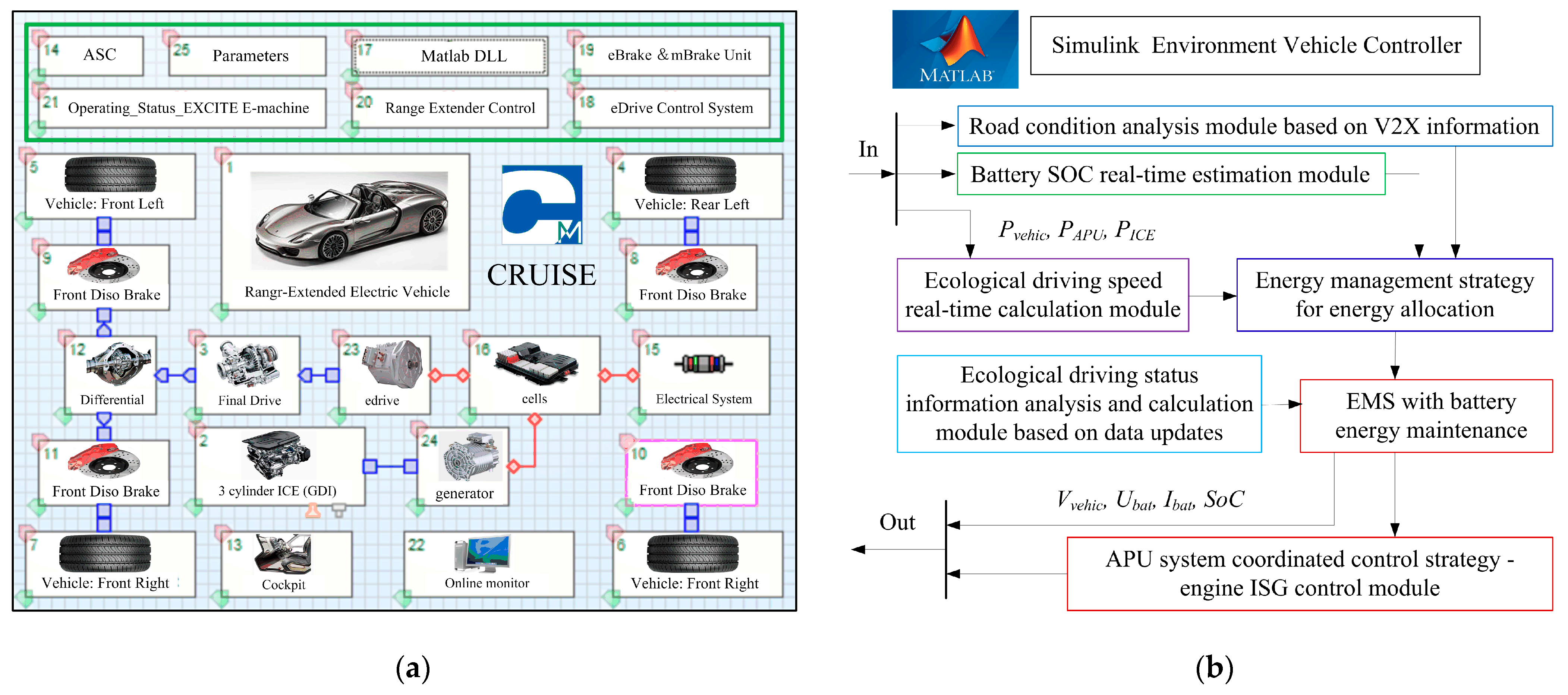
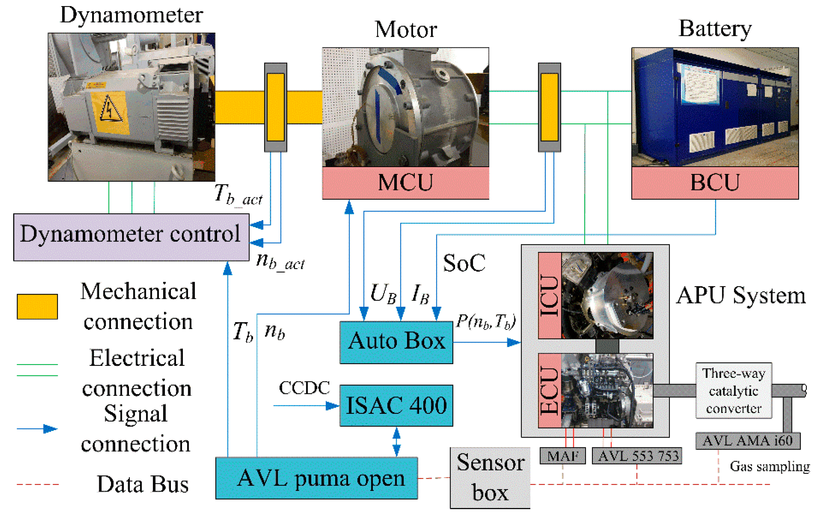
As illustrated in Figure 2, the powertrain of the CAR-EEV is composed of a traction battery, APU, drive motor, mechanical drive mechanism, intelligent information system, and control system. This system was selected by this study as the research object for the design of the EMS.

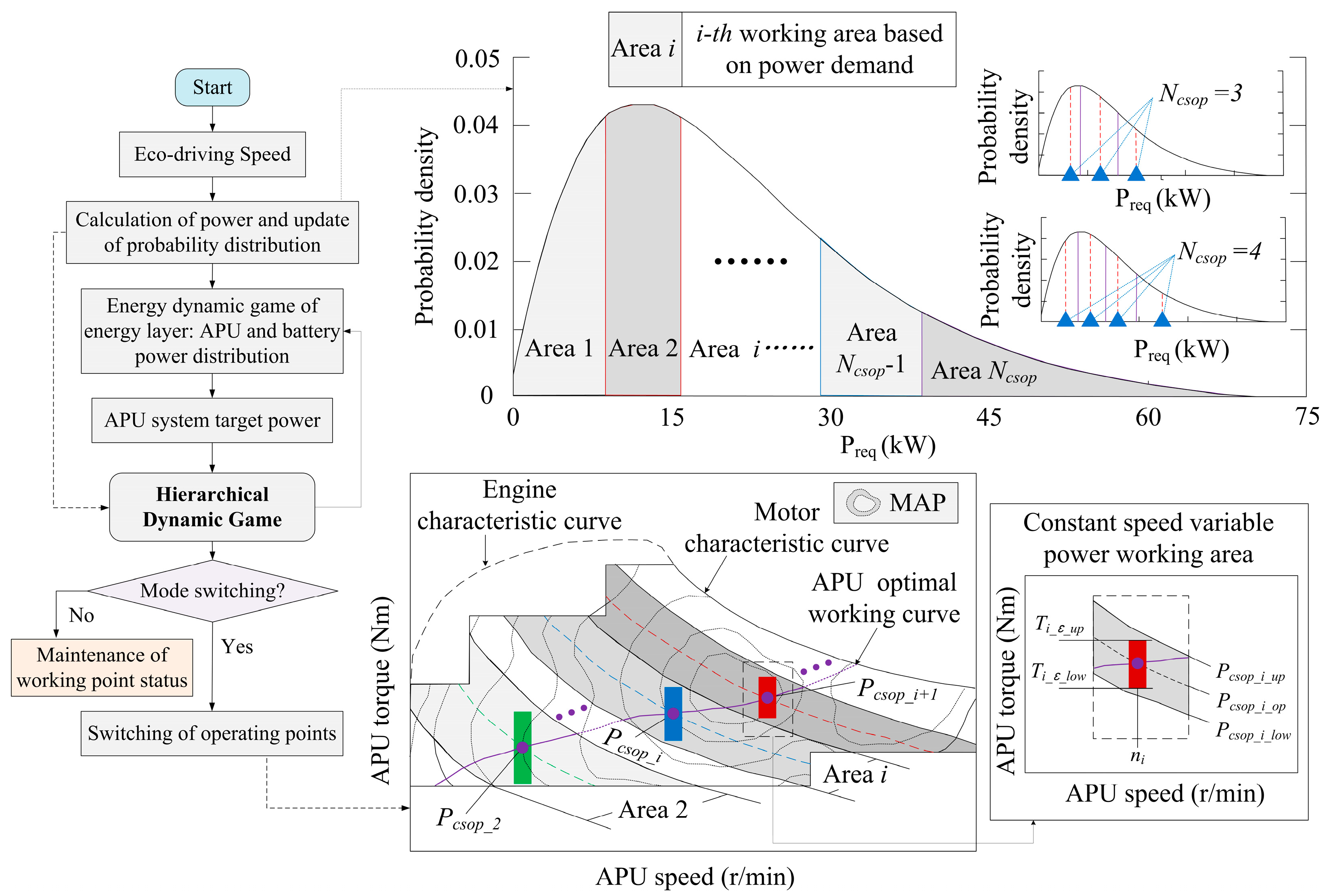
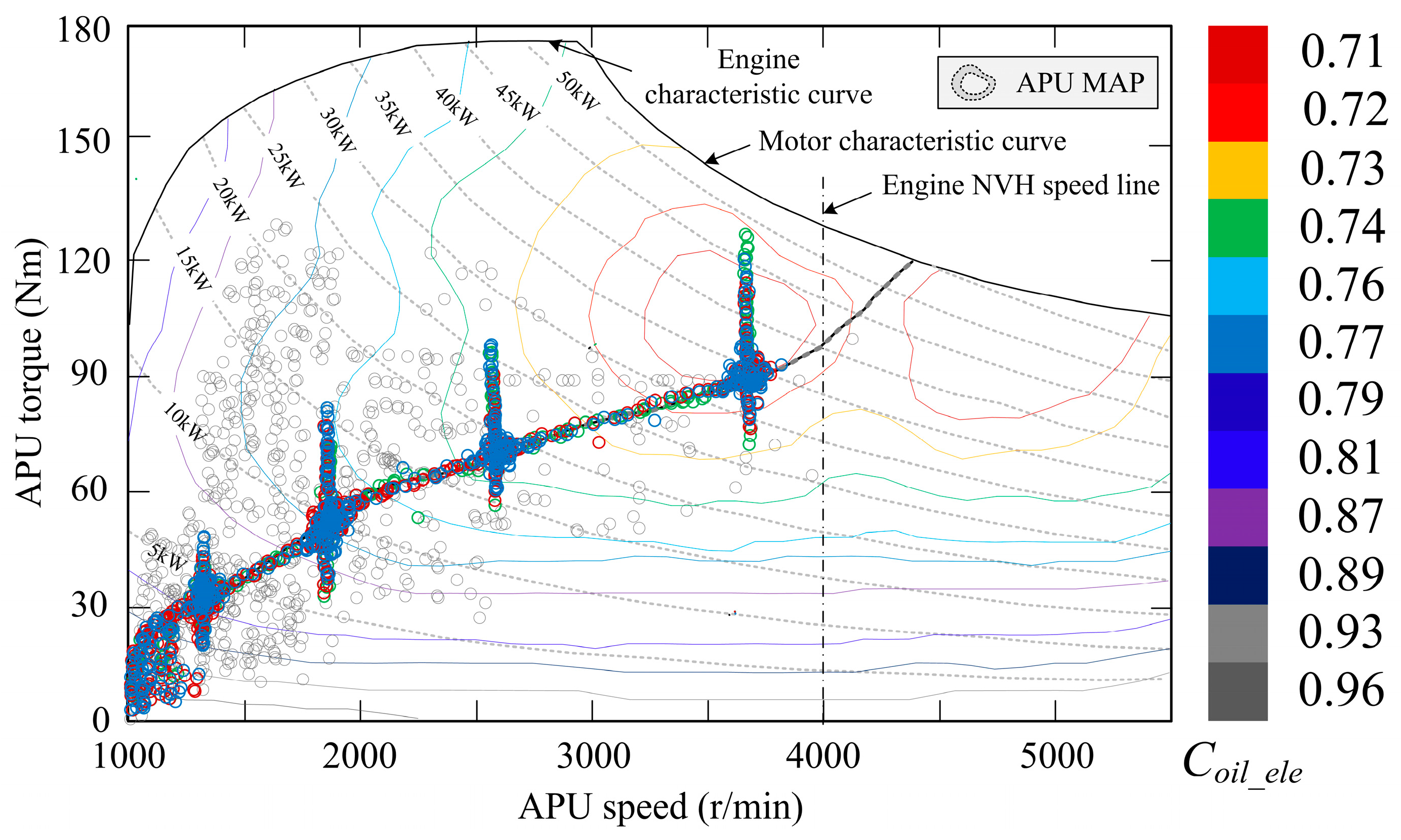
In terms of APU system work-area optimization, there are three types of rule-based APU system power-output forms (work mode/area): namely, fixed-point (constant speed, constant torque), multi-point (constant speed, variable torque) and optimal-curve power following (variable speed, variable torque), as shown in Figure 2. The APU system operates at variable speed and torque on the optimum curve and at constant speed and torque in multi-point mode, both of which allow the APU system to follow the vehicle power requirement. When the operating point speed is considered to be continuous, the APU operating mode changes from single point to multiple points, and the number of operating points increases, to work along the optimal curve, commonly referred to as a power-following strategy. The different operating modes of the APU system can thus be described in terms of the number of APU operating points (N_csop) and the power range (ε_i) at the speed where this operating point is located. Therefore, the operating strategy of the APU system can be structurally described as a decision logic based on N_csop and ε_i: by synergistically optimizing these two dimensional parameters, the system can dynamically switch between fixed-point, multi-point, and power-tracking modes.

The vehicle’s required power P_req is calculated based on the target vehicle speed under the driving cycles, and the distribution range of P_req is statistically analyzed by dividing it into several power ranges. The cumulative power distribution function is obtained as follows:

$$F_p(t)={\displaystyle {\int }_{-\infty }^t{p}_{req}(t)dt}$$

(14)

where F_p(t) is the cumulative power distribution function and p_req(t) is the probability density function of the vehicle’s required power.

The principle of the APU system working area under the power probability density function is shown in Figure 3.

Divide the P_req interval evenly into N_csop sections, with each section corresponding to a constant speed operating point of the APU system. By combining the maximum and minimum power values of the i-th interval and the power fluctuation margin coefficient ε_i, the upper and lower power limits of the APU system at operating speed n_i can be calculated as follows:

$$\left\{\begin{array}{l}{P}_{csop\_i\_up}=P_{csop\_i\_opt}+{\displaystyle \frac{(P_{csop\_i\_\max }-P_{csop\_i\_\min }){\epsilon }_i}{2}}\\ P_{csop\_i\_low}=P_{csop\_i\_opt}-{\displaystyle \frac{(P_{csop\_i\_\max }-P_{csop\_i\_\min }){\epsilon }_i}{2}}\end{array}\right.$$

(15)

$$\mathrm{\Delta }{P}_{i\_\epsilon }=P_{csop\_i\_up}-P_{csop\_i\_low}$$

(16)

$${\epsilon }_i={\displaystyle \frac{\mathrm{\Delta }{P}_{i\_\epsilon }}{P_{csop\_i\_\max }-P_{csop\_i\_\min }}}$$

(17)

where P_{csop_i_max}, P_{csop_i_min,} P_{csop_i_up} and P_{csop_i_low} are the maximum, minimum, upper and lower power in the i-th interval; P_{csop_i_opt} is the power of the APU system operating at the optimal curve; and ε_i is the power fluctuation margin coefficient. ∆P_{i_ε} is the power coverage size. The torque at operating speed n_i in the i-th interval is calculated as follows:

$$\left\{\begin{array}{l}{T}_{i\_\epsilon \_up}={\displaystyle \frac{9550P_{csop\_i\_up}}{n_i}}\\ T_{i\_\epsilon \_low}={\displaystyle \frac{9550P_{csop\_i\_low}}{n_i}}\end{array}\right.$$

(18)

where T_{i_ε_up} and T_{i_ε_low} are the upper and lower torque limits of the APU system operating in the i-th section; the switching thresholds for two adjacent working points are set to

$$\left\{\begin{array}{l}{P}_{i\_cr\_uo}=P_{csop\_i\_\max }\\ P_{i\_cr\_low}=P_{csop\_i\_\min }\end{array}\right.$$

(19)

where P_{i_cr_up} is the APU power threshold when switching between the i-th interval and the i+1-th interval, and P_{i_cr_low} is the APU power threshold when switching between the i-th interval and the i−1-th interval.

Finally, the target power and torque values of the APU real-time operating point are calculated as follows:

$$\left\{\begin{array}{l}{P}_{i\_cr\_up}=P_{csop\_i\_\max }\\ P_{i\_cr\_low}=P_{csop\_i\_\min }\end{array}\right.$$

(20)

$$T_{APU\_act}={\displaystyle \frac{9550 P_{APU\_act}}{n_{APU\_act}}}={\displaystyle \frac{9550 P_{APu\_act}}{n_i}}$$

(21)

where P_{APU_act}, n_{APU_act} and T_{APU_act} are the real-time target output power, speed, and torque values of the APU system, respectively.

The study uses the DP algorithm, which combines the data of engine fuel consumption, emissions, and ISG engine efficiency characteristics to obtain the optimal operating curve of APU system energy-consumption emissions characteristics [6]. Based on this curve, the APU system operating mode/area control strategy is designed.

2.3. Principle of APU Operating Point-Switching Decision Based on Dual Dynamic Game

In order to improve the cognitive intelligence of CAR-EEV vehicle decisions and achieve intelligent vehicle control, in this section the power allocation and the decision as to whether to switch APU operating modes/points are addressed, based on the dynamic game in the context of multi-source V2X information. A feasibility analysis of the APU operating point switch under multi-point modes is also required. If the conditions for switching to the optimal operating point are met, it is necessary to consider whether the APU system can operate continuously for a certain period of time, to better meet the power demand without switching again; because of this conversion, the dual energy source system has better work efficiency after the point is switched [18]. This involves achieving efficient operation of both the APU and battery systems, which enables connected CAR-EEV to engage in multi-step game interactions with V2X, thereby achieving higher system efficiency.

Considering the complexity, non-uniqueness, and coordination of APU multi-point operating modes in the power-following process, an intelligent switching non-cooperative dynamic game decision algorithm is established. Game theory paradigms are used to address potential conflicts between point/mode switches, considering energy consumption, emission reduction, and battery-life friendliness. The detailed modeling of power demand for the powertrain system under complex scenarios is refined into four parts: game benefits that integrate energy-saving and emission reduction, V2X information, reducing battery-capacity decay, and comprehensive performance indicators. Finally, a comprehensive performance index is established, incorporating different weight coefficients and considering vehicle dynamics constraints and road speed limits as the game’s total payoff function or optimization objective. The dynamic game interactive-decision process is unfolded using game trees, and subgame-perfect Nash equilibria for each continuous stage of the game are sought [21]. The potential conflicts during the real-time judgment of APU operating point/mode switches are evaluated. A detailed design of the game-mode switch rule table is developed by combining standardized switching thresholds with whether APU operating-mode switching has been completed. The decision process for the APU system-operating point switching involves current power, target power demand, the span of current speed to target speed (n_i+1−n_i), the demand torque at the current speed, and the span of target torque (T_i+1−T_i). The main factors influencing the speed switching of the APU system include one subjective factor (driving style) and two objective factors (road congestion and battery level). In a multi-source information environment, considering the control target from multiple perspectives, the APU system operating point-switching model is more complex than conventional control modes (based on threshold switching). The most significant difference from conventional operating conditions is the predictability of future driving conditions. Therefore, an intelligent decision system has the opportunity to fully consider the impact of global optimization modes when calculating future power demand and energy management. APU work point-switching strategy based on the dynamic game algorithm is shown in Figure 4. Firstly, it is necessary to determine whether the APU system intends to switch the operating point power: is there a change in the target speed ∆n_i > 0? This is determined by comparing the current APU operating point with the speed difference from the optimal target operating point under power demand to establish the target speed. If the demand for the optimal operating point does not require a speed change, and the operating condition demand duration exceeds a predefined time threshold, it indicates that the target operating point provides sufficient working time and space, and the APU operating point maintains its original working mode. Conversely, if the conditions for game initiation are met, indicating a conflict of interest in whether the APU operating point should switch, a game is initiated. In this case, the dynamic game algorithm of the EMS system is activated. During the game, efforts are made to determine the optimal timing for operating point switching, calculate the payoff function, construct the payoff matrix, solve the optimal strategy combination for the current stage, and choose the target operating speed. Finally, a dynamic game is carried out based on the APU’s multi-point strategy selection, until the termination conditions of the game are met.

The detailed determination processes of the utility functions and the Nash equilibrium for the two participants have been clearly presented, as follows:

$$C_s=\alpha \cdot \max (0,S-S_{\max })+\alpha \cdot \max (0,S_{\min }-S)$$

(22)

$$C_{cycle-\cos t}=\beta \cdot C_{cycle}\cdot {\displaystyle \frac{\left|P_{battery}\right|}{\eta \cdot P_{\max -battery}}}$$

(23)

$$C_{demand}=\gamma \cdot \max (0,P_{demand}-P_{battery})$$

(24)

where C_s is a state-of-charge maintenance cost, S is the current SoC, S_min, S_max are the target SoC range, α is the penalty coefficient for SoC deviation from the target range, η is the charge–discharge efficiency, β is the impact coefficient of charge–discharge cycles on lifespan, and P_max-battery is the maximum output power of the battery. C_cycle is the calculation formula for the per-cycle cost.

Combining the above three costs, the utility function of the battery (U_battery) can be expressed as

$$U_{battery}=-(C_s+C_{cycle-\cos t}+C_{demand})$$

(25)

Procedure for determining the Nash equilibrium: the strategy space of the battery (with different output powers P_battery, whose value range is [0, P_max-battery]) and the strategy space of the APU (with different output powers P_APU, whose value range is [0, P_max-APU]), and whether to switch operating points are specified; for each strategy combination of the battery and APU, the corresponding utility function values U_battery(P_battery, P_APU) and U_APU(P_battery, P_APU) are calculated, and the payoff matrix is constructed. Then, the iterative method is employed to find the Nash equilibrium.

2.4. Multi-Objective Evaluation Model for EMS Considering Energy Consumption Emissions and Battery Life

While the fixed operation of APU at high-efficiency operating points can reduce energy consumption and emissions, this mode of operation can increase battery usage and shorten battery life. The parameter optimization of the HDGEMS design considers 3 primary objectives, and the HDGEMS described in Section 2 is optimized from a multi-objective perspective. The optimization of the APU system operation mode/area is conducted based on the MOO research framework, in this section, in order to verify whether the proposed MOO method can achieve a better balance among energy consumption, emissions, and battery life. The EMS performance index considers three metrics: the oil–electric conversion loss rate (C_{oil_ele}), comprehensive exhaust emissions (E_com), and the battery-capacity loss rate (Q_loss) [22]. The APU serves as one of the energy sources for CAR-EEV, and all fuel consumption and emissions originate from the engine. This section outlines the evaluation criteria used to assess fuel consumption and exhaust emissions, as follows. Since the engine is mechanically linked to the generator in the APU system, solely considering the engine’s oil consumption characteristics fails to accurately represent the vehicle’s overall energy consumption. Taking into account the engine efficiency, the C_{oil_ele} is calculated as follows:

$$C_{oil\_ele}=1-{\displaystyle \frac{360\cdot {\eta }_{ele}}{{\eta }_{oil}\cdot \rho }}$$

(26)

where η_ele is the power-generation efficiency of the generator; η_oil is the efficiency between fuel and the effective power of the engine; and ρ is the calorific value of petrol, which is 4.6 × 10⁷ J/kg. It is evident that C_{oil_ele} defines the energy-transmission loss rate, and a smaller C_{oil_ele} value corresponds to better fuel economy.

The conventional exhaust gases (CO, CH and NO_x) are considered in the APU comprehensive exhaust-emission characteristic function E_com, and the E_com is calculated as follows:

$$E_{com}={\xi }_{CO}{E}_{CO}+{\xi }_{CH}{E}_{CH}+{\xi }_{N{O}_x}{E}_{N{O}_x}$$

(27)

where E_CO, E_CH and E_NOx are CO, CH and NOx emission characteristic functions and ξ_CO, ξ_CH and ξ_NOx are the weight coefficients of E_CO, E_CH and E_NOx, respectively. [ξ_CO, ξ_CH, ξ_NOx]^T = [0.4, 0.3, 0.3]^T.

Undoubtedly, the repeated charge and discharge cycles of the battery storage system will affect the aging speed of the battery. The optimal charging capacity can be achieved by modifying and controlling the charging-current profiles, and the negative impact of current on battery life can be minimized [23]. The battery-capacity loss rate Q_loss is calculated to evaluate the battery-life model.

Due to the limited space of this paper, this research primarily focuses on the application of Q_loss (for simplicity), and detailed experimental information on the fitting and determination of battery-life model parameters can be found in Ref. [23]. In this article, the fitting parameters in this paper are set as Q₁ = 0.495 and Q₂ = 0.379. The operating temperature is also a crucial factor affecting the battery life. In this study, the battery operating temperature is standardized at 25 °C. Finally, the Q_loss is obtained as follows:

$$Q_{loss}={\displaystyle {\int }_0^{T_{cyc}}0.495\times \frac{d{I}_{bat}(t)}{dt}\times \exp \left(0.379\frac{I_{bat}(t)}{A{h}_{cell}}\right)\times N_{cyc}\times DODdt}$$

(28)

where DOD is the depth of discharge (DOD = 0.7); Ah_cell is the cumulative capacity of the battery; I_bat(t) is the battery current; T_cyc is the total cycle time; and N_cyc is the number of cycles.

In engineering practice, determining the preferred solution is critical. In this paper, the linear normalization method is selected for optimal decision, which is a practical and efficient multi-objective normalization optimization method, and can clearly reflect the weight assigned to the optimization objective. In addition, it is necessary to standardize the cost function for each dimension before using the linear normalization method. Furthermore, the three objective functions, C_{oil_ele}, E_com and Q_loss possess different physical connotations. In order to reach the final quantitative decision, these objective functions need to be combined into a one-dimensional cost function. This study adopts a multi-objective normalization method and uses the following normalization formula:

$$X^{(nor)}={\displaystyle \frac{X_p-{X_p}^{(\min )}}{{X_p}^{(\max )}-{X_p}^{(\min )}}}$$

(29)

where X^(nor) is the normalized result of the objective function; X_p is the original data in the Pareto optimal solution set; and X_p^(max) and X_p^(min) are, respectively, the maximum and minimum values of the original data in the Pareto optimal solution set.

The comprehensive optimal performance function of the APU system, called the optimal comprehensive vehicle performance (I_{com_ovp}), is defined as follows:

$$I_{com\_ovp}={\displaystyle \frac{1}{{\omega }_C{C}_{oil\_ele}+{\omega }_E{E}_{com}+{\omega }_Q{Q}_{loss\_batt}}}$$

(30)

where I_{com_ovp} is the comprehensive performance evaluation index; ω_C, ω_E, and ω_Q, respectively, represent the weight coefficients assigned to C_{oil_ele}, E_com, and Q_{batt_loss}.

C_{oil_ele} defines the energy-transmission loss rate, and a smaller C_{oil_ele} value corresponds to better fuel economy. E_com reflects the comprehensive emission level, and a smaller E_com value corresponds to better exhaust quality. Q_{batt_loss} is used to quantify the degree of performance degradation during battery use, including capacity degradation, internal resistance increase, etc., reflecting its remaining usable life. The selection of weight coefficients plays a crucial role in determining the final results. Based on the hierarchical analysis method [24], the multi-objective evaluation matrix is obtained as shown in

Table 1. Multi-objective Evaluation Matrix C_{oil_ele}, E_com and Q_{batt_loss}.

Evaluation Matrix	Coil_ele	Ecom	Qbatt_loss
Coil_ele	1/1	4/1	2/3
Ecom	1/4	1/1	1/4
Qbatt_loss	4/3	7/2	1/1

, and the weight vector result is calculated as [ω_C, ω_E, ω_Q]^T = [0.41, 0.13, 0.46]^T. This result becomes an important reference for the selection of weight coefficients. It should be noted that considering the catalytic conversion effect of the three-way catalyst weakens the relationship between the exhaust-emission level and the direct engine-emission content. Therefore, the weight factor of E_com is relatively small, while the weight factors of C_{oil_ele} and Q_{batt_loss} are comparable. It is worth mentioning that different multi-objective evaluation matrices will produce different weight factors. In this study, the selected weight parameters are [ω_C, ω_E, ω_Q]^T = [0.4, 0.2, 0.4]^T. The source of the matrix elements is determined by inviting experts and combining design experience with the AHP scaling method to compare and score each indicator pairwise, and then calculating the geometric mean to obtain the matrix elements.

3. Results and Discussion

By means of simulation tests and experimental bench tests, the energy management strategy proposed in Section 2 is validated in this section, and the effectiveness of HDGEMS and the proposed MOO method in achieving the optimal balance between energy consumption, emissions, and battery life is confirmed.

3.1. Optimizing the Vehicle Model

The vehicle-dynamics model and the proposed HDGEMS are created in AVL/Cruise (2019) software and MATLAB/Simulink (R2022a) software, respectively; the co-simulation model is shown in Figure 5.

At the initial stage of the simulation, a vehicle dynamics model is established in the AVL/Cruise software, and various vehicle parameters—such as mass, dimensions, and powertrain characteristics—are inputted. Subsequently, the proposed HDGEMS model is constructed in MATLAB/Simulink, including the eco-driving speed module, dynamic game module, and other relevant components. Initial conditions for co-simulation are set, such as initial vehicle speed and initial battery SoC. High-performance workstations are adopted as the hardware for the simulation, which can meet the requirements of massive data calculation and model operation during the co-simulation process. To ensure the accuracy and reliability of the simulation results, key data obtained from the simulation (e.g., vehicle speed and power) are compared and analyzed with the test data of actual vehicles under the same or similar driving scenarios, and the accuracy of the vehicle dynamics model is verified. The results derived from the aforementioned simulation platform are illustrated in Figure 6. The dynamically varying vehicle speed and increasing mileage under eco-driving reproduce the actual driving conditions, and the distribution of the APU system’s operating area under the multi-point strategy reflects its operating status under diverse power demands, which provides critical basis and support for subsequently verifying the balance effect of the HDGEMS and the proposed MOO method among energy consumption, emissions, and battery life.

3.2. Comparative Analysis and Discussion of Experimental Results

To verify the universality and compare the optimal effect of the HDGEMS with the dynamic game algorithm, tests were carried out by simulation to determine the efficiency of the proposed strategy. To test the universality and compare the optimal effectiveness of the HDGEMS, the HDGEMS with the Eco-driving Speed module (EMS_he-dg) and the HDGEMS with the Eco-driving Speed module off (EMS_heoff-dg) are selected for comparative study. The EMS_heoff-dgoff without the Eco-driving Speed module is expressed as a revision strategy (EMS_he-dg), and the HDGEMS without the Eco-driving Speed module (EMS_heoff-dg) and the HDGEMS without the dynamic game (EMS_he-dgoff) were set as control groups. As a result, many more APU power transients can be observed throughout the CS phases, and the detailed results of the optimization of the performance for the different APU operating modes are shown in

Table 2. Test results of performance of the HDGEMS with dynamic game and adaptive adjustment module.

HDGEMS	Module Status		Evaluation Index
	Eco-Driving Speed	Dynamic Game	Coil_ele	Ecom	Qbatt_loss	Icom_ovp
EMSheoff-dgoff	Off	Off	0.727	0.545	12.1%	0.77
EMSheoff-dg	Off	On	0.723	0.538	11.3%	0.81
EMShe-dgoff	On	Off	0.724	0.536	10.8%	0.83
EMShe-dg	On	On	0.718	0.532	9.3%	0.86

Note: all parameters listed in this table (C_{oil_ele}, E_com, Q_{batt_loss}, I_{com_ovp} ) are dimensionless indices.

and Figure 7.

When comparing EMS_heoff-dgoff with EMS_he-dg, the latter always has a visible advantage in terms of APU work-point adaptability. This better adaptability is reflected in three aspects. (1) The APU system is controlled at more efficient and better operating points, due to the real-time control performance of the eco-driving speed algorithms, resulting in better economics. (2) The role of dynamic algorithms in intelligent real-time decision-making of operating point-switching time can enable more power-following points to work in high-efficiency areas, to realize better economic performance, While a higher frequency of operating point switching may elevate energy consumption and emissions, this involves a subtle balance and trade-off. (3) The dual objectives of “power enhancement and fuel consumption reduction” are accomplished by extending battery-discharge cycles. While energy efficiency is enhanced, precise tracking of the battery SoC reference curve is concurrently secured, thereby sustaining current stability. By virtue of an appropriate discharge state, energy loss induced by DOD is effectively mitigated, and battery service life is significantly prolonged. It is noteworthy that, analogous to the EMS_he-dg technology, although some APU operating points and energy distribution modes during cycle advancement are adjusted to optimize the I_{com_ovp} index, electrical energy remains efficiently utilized up to the cycle termination.

3.3. Experimental Results Considering Different Operating Modes of the APU System

As shown in Figure 8, operating-point distribution MAPs for the APU under four strategies are acquired, where the gray, red, and blue hollow circles in the figure denote the operating-point distribution results of the traditional APU system power following modes (EMS_pfm), EMS_heoff-dgoff and EMS_he-dg, respectively.

As shown in

Table 3. Test performance results of the different APU operating modes in HDGEMS.

HDGEMS	APU Operating Modes	Evaluation Index
		Coil_ele	Ecom	Qbatt_loss	Icom_ovp
EMSpfm	power following	0.765	0.653	13.1%	0.66
EMSheoff-dgoff	Ncsop = 3	0.734	0.567	12.5%	0.73
EMShe-dg	Ncsop = 3	0.727	0.542	10.8%	0.77
EMSheoff-dgoff	Ncsop = 4	0.731	0.547	11.5%	0.79
EMShe-dg	Ncsop = 4	0.720	0.518	9.3%	0.81

Note: all parameters listed in this table (C_{oil_ele}, E_com, Q_{batt_loss}, I_{com_ovp}) are dimensionless indices.

, in modes N_csop = 3 and N_csop = 4, the APU system can be operated in the corresponding constant-speed and variable-torque operating regions, according to the strategy rules, to respond to the demand power. The distribution of operating points is uniform, the fluctuation of operating speed is small, and the operating points can be operated closer to the optimal operating curve. The statistical results show that under the EMS_he-dg, 27.1% of the APU’s original operating points are switched to optimal operating points compared to the EMS_heoff-dgoff. The control results regarding energy consumption, emissions, and battery capacity loss are presented in Table 3.

It is clear that the EMS_he-dg strategy is superior to the EMS_heoff-dgoff strategy, giving better control results in terms of energy consumption, emissions, and battery-capacity loss. The overall evaluation index I_{com_ovp} is substantially improved. When the output power of the APU is insufficient to satisfy the vehicle’s demand, the excess electrical energy will be subjected to secondary conversion for battery power supply. By means of regulating the APU operating points via the EMS, the balance between the deviation from the optimal operating point, dynamic operating-point switching, and the achievement of secondary charging can be attained. The primary source of efficiency loss stems from the APU’s deviation from its optimal operating point, rather than the energy loss associated with secondary charging. Through the utilization of speed sequence information related to driving characteristics, the optimal strategy can be achieved. By adopting the dynamic game algorithm based on V2X information and the eco-driving speed module, the distribution of power between the APU and the system of battery can be precisely modulated, which not only allows the APU system to operate stably at its optimal operating point, but also minimizes, to the greatest extent, the losses associated with secondary charging and the dynamic-time overhead incurred during APU-operating point switching.

The control strategy proposed in this paper demonstrates prominent efficacy in energy consumption, emissions, and battery life. As noted in the prior study [25], DP functions not only as the optimal offline benchmark, but also as the optimal control approach, taking I_{com_ovp} as its objective function. Given the discrepancies in units and magnitudes across the various performance indicators, the normalization parameters for these indicators will be computed first, to enable the horizontal comparison of the strategies. The computational methods for these parameters are outlined as follows:

$${\mu }_{ik}={\displaystyle \frac{I_{ik}-{I_{ik}}^{\min }}{{I_{ik}}^{\max }-{I_{ik}}^{\min }}}$$

(31)

where μ_ik is the normalized index of the k-th evaluation index on i-strategy; I_ik is the index value; and I_ik^min and I_ik^max are the minimum and maximum values of the index.

The data employed for the normalization analysis in this study comprises two categories: one refers to the simulation results of the aforementioned strategies, and the other denotes the single-objective data derived from the Pareto solution set. The statistical results post normalization processing are illustrated in the Figure 9. It can be observed from the figure that the HDGEMS scheme proposed in this study demonstrates the most exceptional performance. By employing two independent APU operation modes for comparative analysis, respectively, the disparities in performance can be visualized more distinctly; the results reveal that the performance of the two modes is largely consistent. This suggests that the EMS_he-dg scheme proposed in this study attains a sophisticated balance among the three objectives. This control strategy yields exceptional performance in energy consumption control, emission optimization, and battery-lifespan management. Notably, the substantial mitigation of battery-life degradation enables a significant reduction in the overall vehicle in an economical way.

To explore the degree of influence of different variables on EMS results, thereby identifying the most critical influencing factors and providing directions for subsequent optimization and in-depth research, sensitivity analysis was conducted in the study; the initial battery SoC and APU system power limit were selected as key variables, with multiple different initial SoC levels (specifically, 0.2, 0.4, 0.6, and 0.8) set and other conditions kept unchanged. The results indicate that the initial SoC has a relatively significant impact on energy consumption and battery life: when the initial SoC is low, the APU system needs to start more frequently and output higher power to meet vehicle driving demands, leading to increased energy consumption, while the number of charge–discharge cycles of the battery increases and the degree of deep discharge (DOD) intensifies, accelerating battery aging; conversely, when the initial SoC is high, the startup frequency of the APU system decreases, energy consumption is relatively reduced, and the battery-discharge process is gentler, which is beneficial for extending battery life. However, the impact of initial SoC on emissions is relatively minor, as emissions are mainly related to the operating efficiency and combustion status of the APU system. For the variable of APU system power limit, different power limit values (such as 30 kW, 40 kW, 50 kW, and 60 kW) were set, and simulation results show that the APU system power limit has a significant impact on energy consumption and emissions. When the power limit is low, the APU system cannot provide sufficient energy in response to high power demands, resulting in insufficient vehicle power, which necessitates frequent adjustments to the operating mode and increases energy consumption and emissions; when the power limit is excessively high, the APU system may operate in low-efficiency regions under certain working conditions, which also increases energy consumption and emissions. In terms of battery life, a moderate power limit can reduce the charge–discharge pressure on the battery while meeting vehicle power demands, which is conducive to extending battery life. The speed-adjustment threshold in the eco-driving speed algorithm is also a key variable; simulations were conducted with different threshold settings, and the results show that the threshold directly affects the distribution of operating points and switching frequency of the APU system. A smaller threshold causes more frequent adjustments to the operating points of the APU system, and although this can make the vehicle closer to the eco-driving speed, to a certain extent, it increases the switching frequency of the APU system’s operating points, which may lead to increased energy consumption and emissions. The frequent charge–discharge of the battery can also affect its service life: a larger threshold results in relatively stable operating points of the APU system, but may fail to fully utilize the advantages of the eco-driving speed algorithm, thereby affecting the optimization effect on energy consumption and emissions.

3.4. Implementation of Experimental Test and Its Results

The results demonstrate that performance is significantly affected by different EMSs, and further verification needs to be completed on the AVL test bench. The configuration of the test bench is depicted in Figure 10, while

Table 4. Parameters of the vehicle components of the experimental platform.

Components	Parameters	Value	Components	Parameters	Value
Engine	Maximum power/(kW)	65	Battery	Continuous discharge capacity (C)	2
	Minimum speed/(r/min)	950		Nominal voltage/(V)	320
	Maximum speed/(r/min)	6500		Capacity/(A·h)	25
Generator	Maximum power/(kW)	60	Motor	Peak power/(kW)	75
	Maximum speed/(r/min)	9000		Maximum speed/(r/min)	9000

provides the parameters of the components. It should be noted that to ensure the reliability and repeatability of the results, 10 simulation runs are conducted separately for the cases adopting the HDGEMS, the MOO method, and traditional energy-management strategies, and the average value of the 10 simulation results is calculated to represent the central tendency of the energy consumption, emission, and battery-lifespan indicators.

The specific experimental procedure is as follows: first, the parameters of vehicle and the preset driving cycle (CCDC) are entered into the road-load simulation software. Subsequently, the engine and dynamometer are respectively controlled for speed and torque by the AVL system, to simulate the vehicle’s road load. The P_req calculated in real time incorporates the influencing factors of DC bus voltage and current, comprehensively. Next, the battery SoC is collected by the control system, the HDGEMS is implemented, and the target engine speed and target generator torque are output. Finally, power output is achieved by means of the coordinated control strategy (APU). To verify the power trajectory tracking effect, the calculated power output is used as the target power in the experiment. Due to the differences in the final state of charge among the three strategies, it is unreasonable to directly evaluate the fuel consumption values. The comparison of the 100 km equivalent fuel consumption (Ge) of the three control strategies after adjusting the final SoC (the fuel efficiency under the corrected SoC) is shown

Table 5. Test performance results of the different EMS.

Strategy	Ge (L/100 km)	∆Ge	Coil_ele	∆Coil_ele	Ecom	∆Ecom	Qbatt_loss	∆Qbatt_loss
EMSpfm	4.78	−	0.731	−	0.532	−	14.2%	−
EMSheoff-dgoff	4.33	−9.41%	0.723	−1.09%	0.513	−3.57%	10.8%	−23.9%
EMShe-dg	4.12	−13.8%	0.719	−1.64%	0.508	−4.51%	9.4%	−33.8%

Note: all parameters listed in this table (C_{oil_ele}, ∆C_{oil_ele}, E_com, ∆E_com, Q_{batt_loss}, ∆Q_{batt_loss}) are dimensionless indices.

.

The total consumption of EMS_he-dg is slightly lower than EMS_pfm by about 13.8%, and EMS_he-dg is slightly better than EMS_heoff-dgoff. And it is observed that the fuel consumption results (Ge, C_{oil_ele}) of the three control strategies are comparable. Owing to the fact that the power demand of the EMS_pfm system undergoes dynamic fluctuations and remains relatively high, considerable potential for optimization remains. The experimental results show that there is a significant difference in fuel consumption between the EMS_heoff-dgoff and the EMS_he-dg, indicating that the proposed EMS_he-dg performs well in fuel savings. Compared with the EMS_pfm, the EMS_heoff-dgoff and EMS_he-dg reduced the amount of ecosystem by approximately 3.57% and 4.51%, respectively, demonstrating that the EMS_he-dg can achieve higher emission quality. On the other hand, EMS_pfm has relatively poor emission quality, due to frequent changes in APU operating points. The proposed EMS_he-dg effectively reduces the number of switches by adjusting APU operations to the optimal efficiency range, which is the main reason for its overall consumption reduction. Compared with the EMS_pfm, the EMS_heoff-dgoff and EMS_he-dg significantly reduced Q _loss by approximately 23.9% and 33.8%, respectively. In terms of battery life, when the battery capacity of CAR-EEV drops below 80% of the new battery state, it can be considered as the end of battery life. Under the current proposed configuration, the battery life is approximately 1.8 times longer than traditional rule-based strategies that do not consider V2X information during travel. The experimental results are consistent with the simulation conclusions. In addition, the proposed EMS_he-dg has been optimized by adjusting the APU operating point to reduce battery-capacity degradation rate, thereby further extending battery life. Through a comprehensive analysis of the three aforementioned factors, notable differences are identified between the two strategies. The research outcomes confirm the feasibility of the proposed energy management scheme. With the support of the parameter adjustment module based on MOO, the proposed HDGEMS system facilitates comprehensive optimization of vehicle performance (achieving a favorable balance across multiple objectives), with a significant improvement in overall performance. This research and the optimization approach provide a more practical reference for the design optimization of EMCS.

4. Conclusions

In order to achieve the optimal energy allocation of two energy sources of CAR-EEV from a multi-objective perspective, an HDGEMS is introduced and a dynamic game optimization method based on V2X information is proposed in this paper. It holds pioneering significance in achieving multi-objective optimal energy distribution, and the long-standing challenge that traditional methods struggle with to balance economy, emission reduction, and battery life has been effectively addressed. The proposed HDGEMS showed good performance by implementing a dynamic game- and parameter-adaptive algorithm for the fuzzy algorithm. Through the real-time optimization of ride-comfort evaluation indicators for road conditions, dynamic adjustment of power distribution between the APU and the battery can be realized. This thereby enables the APU to operate efficiently under optimal operating conditions, and ultimately minimizes energy losses during secondary charging and dynamic switching of the APU, to the maximum extent. This model allows the current operating point under APU multi-point modes to engage in multi-step game interactions with the target operating point, thereby achieving greater energy-saving and emission-reduction potential, higher battery operational efficiency, and better longevity characteristics. The results show that when comparing EMS _wdg-wadm with EMS _dg-adm, the latter always has a visible advantage in terms of APU work-point adaptability. The simulation and experimental results indicated that economic improvement, emission reduction, and prolonging the battery life of CAR-EEV were kept in balance effectively, under the control of the proposed HDGEMS, with the intelligent optimization method. The design and the related conclusions obtained from the study lay the research foundation for the implementation of the top-level intelligent mode-switching-based energy management strategy for optimal energy allocation. In terms of data acquisition, the V2X information relied on in the study may be inaccurate or delayed, which impairs the real-time performance and accuracy of the dynamic game-based optimization method. In practical applications, significant differences exist in road conditions and traffic rules across different regions, posing challenges to the universality of the model and making it difficult to achieve optimal energy distribution in all scenarios. For subsequent research, targeted improvements should be made to the data acquisition method and the universality of the model, to address these limitations.