Structural Damage Detection Using Adversarially Calibrated Simulations and Deep Learning from Frequency-Domain Signals

Abstract

Structural Damage Detection is an area that is becoming increasingly important as structure age and become more prone to failure. Early identification of these changes can lead to significant cost savings and potential damage reduction. Conventional data-driven methods typically require large datasets from both damaged and undamaged structural states, which can be difficult or even impossible to collect in real-world situations. Meanwhile, purely model-based techniques often face challenges in accounting for real-time environmental variations and the complexities of structural behavior. To address this limitation, the proposed methodology in this paper employs a hybrid system that utilizes structural models to generate training data for various structural scenarios, using a methodology based on the concepts of Generative Adversarial Networks to find the optimal excitation parameters for the model, aiming to produce response levels as close as possible to those obtained experimentally. This data serves as input for training algorithms to classify the structural condition based on the frequency information of temporal acceleration signals. The results show that the neural-based computational learning techniques are able to achieve efficiency rates above 99% in damage localization and almost 97% in severity estimation over 2 min-long experiments on a four-story lab-scale shear building.

1. Introduction

Structural alteration in slender structures can be attributed to diverse factors, encompassing design and construction issues, operational conditions, severe natural events, and natural aging [1]. In most cases, modifications in structures may be associated with damage and, when damaged, the material properties change, adversely affecting the stiffness, stability and operational life of the structure [2,3]. Traditional damage assessment methods, reliant on periodic visual inspections, often prove inefficient for complex structures, which require highly qualified personnel and unobstructed access to the monitored structural elements [4,5]. Consequently, considerable research efforts have been directed towards the development of automated local and global Structural Health Monitoring (SHM) and Structural Damage Detection (SDD) techniques [6,7]. SHM is a broad and highly interdisciplinary research field that encompasses experimental testing, system identification, data acquisition and management, and the continuous monitoring of environmental and operational conditions over extended periods [8,9]. The most critical component of SHM is damage detection, which is defined as a systematic and automatic process of identifying the existence of a damage, and then localizing and assessing the severity of it [10].

A large number of techniques have been developed to detect, localize, and quantify structural damage in an attempt to make the monitoring process more feasible [7,11,12]. Vibration-based SDD methods are extensively used in the recent literature to evaluate the global performance of the monitored structure [13,14,15]. These methods involve translating the structure’s vibration response, registered through a network of accelerometers, into meaningful metrics that accurately account for the current condition of the structure [16]. A wide variety of vibration-based SDD systems have been developed in the field of structural SHM [17,18,19,20]. The primary objective of these systems is to address the limitations associated with conventional SDD approaches by providing a systematic, feasible, and consistent way of identifying the presence, location, and severity of structural damage based on the vibration response of the monitored structure [21,22,23].

Within vibration-based techniques, a parametric (model-based) or non-parametric (data-based) approach can be adopted [24]. Model-based techniques involve the identification of the structural model at a specific state and its subsequent comparison with the model of the undamaged structure in order to identify and locate the modifications that it suffered [25]. By analyzing the deviations between the identified model and the reference undamaged model, these techniques provide valuable insights into the presence and localization of structural alterations [26,27,28,29]. On the other hand, data-based approach relies on statistical methods to identify damage directly from the measured signals. Unlike model-based techniques that involve comparing structural models, the data-based approach focuses on analyzing the raw data acquired from sensors or measurement devices. Through advanced statistical analysis, such as signal processing techniques, machine learning (ML) algorithms, or pattern recognition methods, the data-based approach aims to extract relevant features or patterns from the measured signals that are indicative of structural damage. By bypassing the need for a detailed structural model, this approach offers the advantage of being more flexible and adaptable to various types of structures, making it suitable for real-time monitoring and detection of damage in complex and evolving structural systems [30,31,32,33,34].

Over the past few decades, computational learning methods have gained significant prominence as an effective tool for addressing structural damage assessment challenges [35]. Consequently, a diverse range of vibration-based SDD systems, encompassing both parametric and non-parametric approaches, have been proposed for civil structures. These computational learning methods have revolutionized the field of SDD by enabling accurate and reliable detection of structural damage through the analysis of vibration data [36,37]. Computational learning algorithms function as classifiers, aiming at discerning different levels of damage by utilizing data characteristics extracted from dynamic responses. By making use of various data processing techniques, these classifiers analyze the extracted features and make informed judgments regarding the severity or extent of structural damage. This approach allows for the automated identification and categorization of damage levels based on the extracted data characteristics, enabling efficient and objective assessment of structural health. A substantial body of research has been devoted to conducting comprehensive analytical and experimental studies aimed at demonstrating the efficacy of ML-based SDD systems, and these systems have been reviewed on multiple instances in recent years [35,38,39,40,41,42], including Deep Learning (DL) methods, which consist of highly complex neural network frameworks capable of automatically learning and extracting intricate features from data [43,44,45,46,47].

Focusing on non-parametric methods, feature extraction remains an important element of the process. This entails the utilization of signal processing techniques to extract damage-indicative features from raw signals. These techniques encompass a range of approaches, including the application of simple statistical measures [48,49], the utilization of principal component analysis [50,51,52], the implementation of wavelet transforms [53], and the option to bypass the feature extraction step altogether and employ raw dynamic data directly as input for the data-based method [16]. By employing these techniques, non-parametric methods enable the extraction and utilization of pertinent information encoded within the raw signals, facilitating the detection and characterization of structural damage. Regarding the specific ML models employed in non-parametric algorithms as classification techniques, a wide range of models has been investigated and applied, including Artificial Neural Networks (ANNs) [53,54,55,56], Singular Value Decomposition (SVD) [57], Support Vector Machines (SVMs) [58,59], polynomial regression [60], or One-Dimension Convolutional Neural Networks (1D-CNNs) [16]. Previous investigations have demonstrated that non-parametric methods excel at distinguishing damage scenarios that cannot be readily attributed to changes in modal parameters [61].

These methods applied to Structural Damage Detection face several limitations and challenges in spite of their flexibility and strong classification abilities [52,55]. A major issue arises from their reliance on feature extraction, as the selection and design of the features can strongly influence the performance and robustness of the method. This can also make the process sensitive to noise levels, signal quality, and preprocessing parameter tuning [57,60], which may affect the stability and reliability of the extracted damage metrics. In addition, although bypassing feature extraction and using raw data has gained attention, these approaches usually require more complex machine learning architectures, increasing computational cost and data requirements.

Most data-driven approaches rely on supervised algorithms, which require labeled data from both damaged and undamaged structural states—a significant limitation given the practical difficulty of obtaining damaged-state measurements. To overcome this issue, this work introduces a hybrid methodology in which an updated structural model is used to simulate undamaged and damaged conditions, providing the necessary datasets for a supervised ML/DL classifier. This strategy eliminates the need for real damage data and avoids complex feature extraction procedures. The main contributions of the method are as follows: (1) the ability to identify both the location and severity of structural damage using vibration signals; (2) the use of ambient, unmeasured excitations during diagnosis, with a heuristic optimization algorithm accurately modeling the system’s energy input; and (3) the generation of all damage scenarios through simulations while still achieving nearly 100% accuracy in damage localization and severity estimation in the examined cases.

The rest of the manuscript is structured as follows. First, Section 2 describes the structure used throughout this work. Then, Section 3 provides details about the proposed SDD hybrid methodology. Subsequently, the experimental results are shown in Section 4. Finally, Section 5 provides some final remarks and conclusions.

2. Case Study

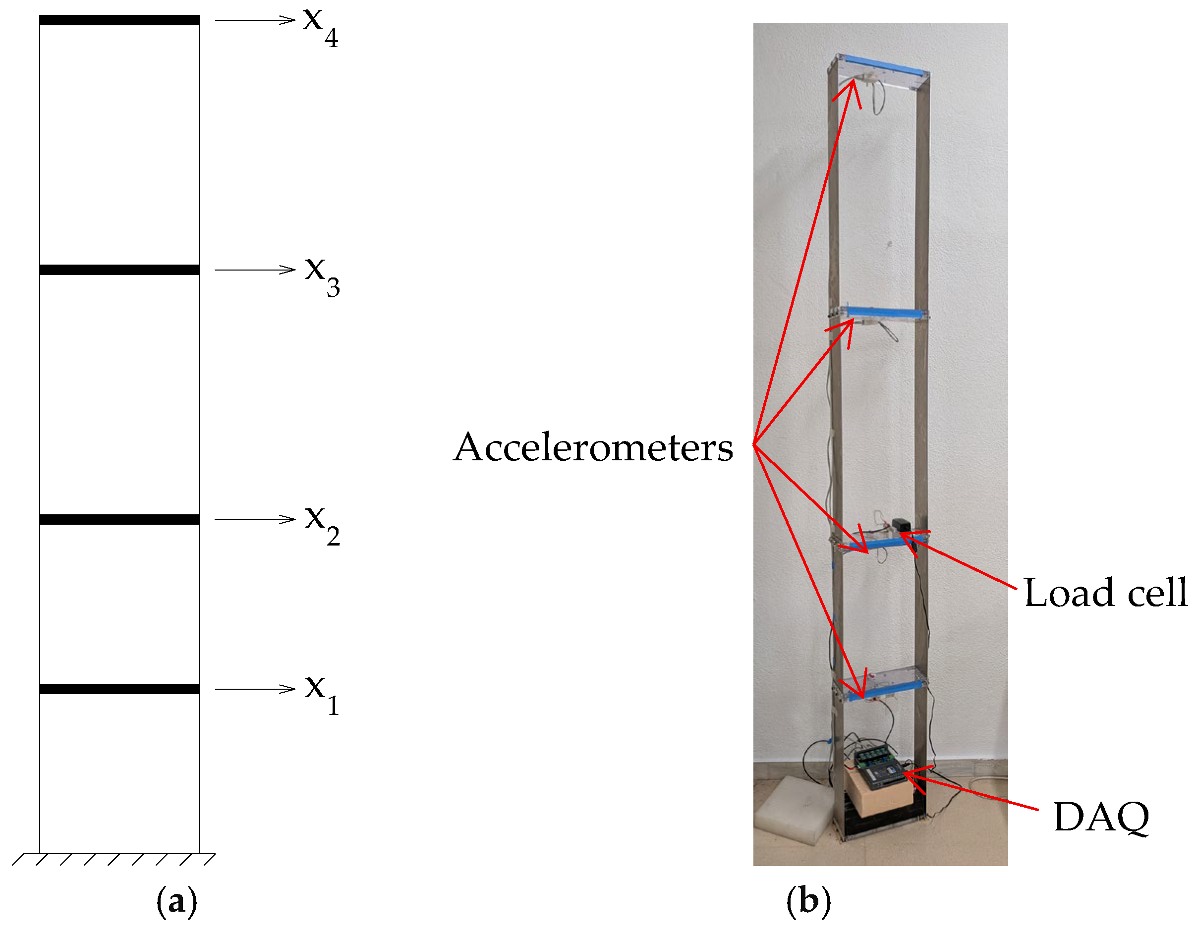
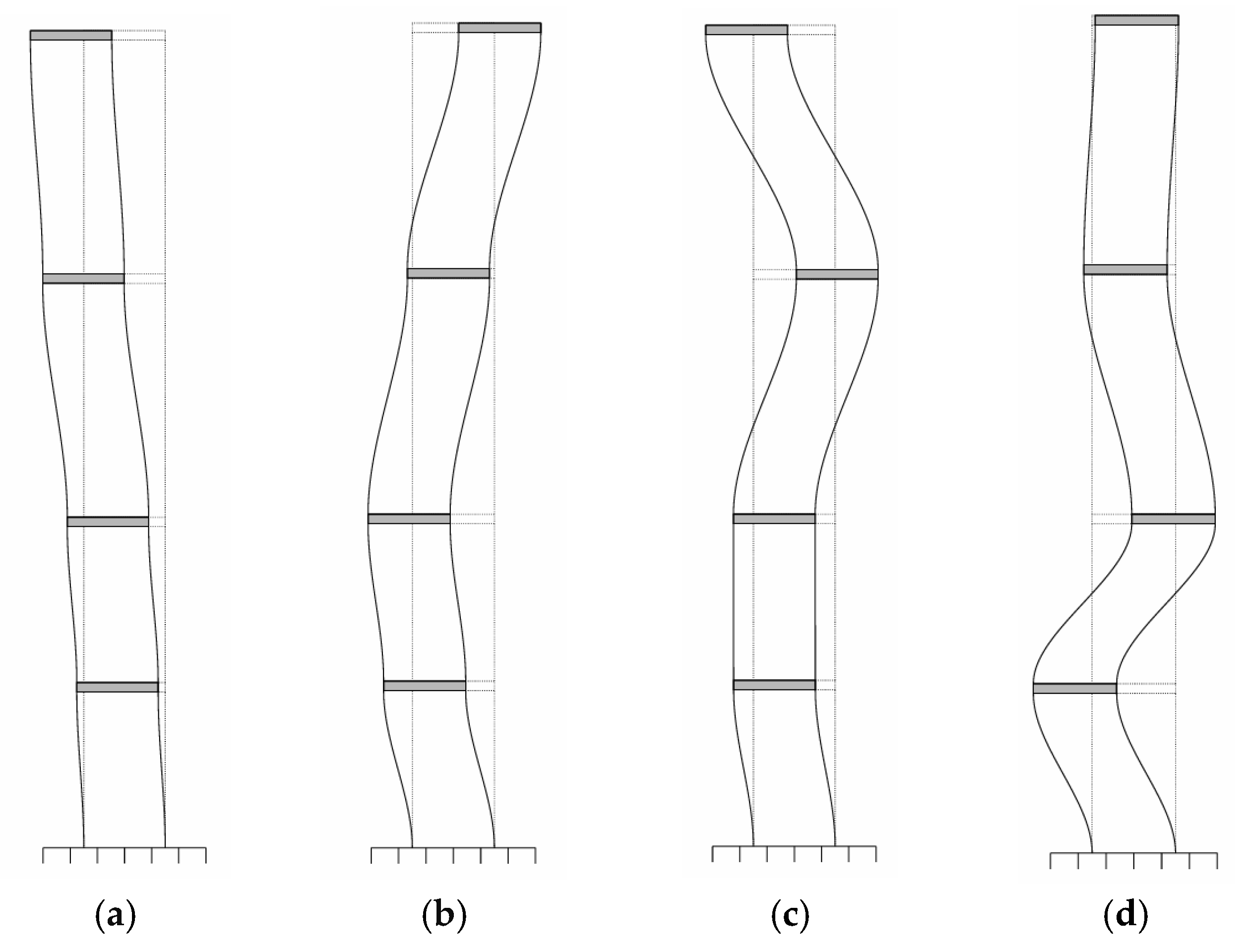
The proposed methodology has been implemented in a laboratory-scale structure consisting of a four-story shear building. Figure 1 shows a conceptual sketch and a picture of the structure under study. It consists of 2 mm thick and 10 cm wide aluminum panels separated by 30 cm, and 10 × 1 × 30 cm methacrylate plates that function as the base of each of the floors. These plates are supported on the aluminum panels with steel screws, on which the magnets that hold the accelerometers are placed. The building is a modular and configurable structure composed of two modules of 0.75 m in height and two others of 0.5 m, resulting in the lumped-mass system depicted in Figure 1. Figure 2 shows the mode shapes of the structure, identified through Experimental Modal Analysis techniques, as explained in Section 3.1. The natural frequencies at which these mode shapes appear depend both on the stiffness (${\mathrm{k}}_{\mathrm{i}}$) and mass (${\mathrm{m}}_{\mathrm{i}}$) of each floor. Any changes in ${\mathrm{k}}_{\mathrm{i}}$ or ${\mathrm{m}}_{\mathrm{i}}$ from the original value are taken as structural changes which, like damage, causes the natural frequencies to change. In this study, structural damage is defined specifically as the changes in the mass of the different floors of the building. Therefore, the damage location procedure consists of identifying the potential change in the mass of some of the floors. Note that, although the stiffness could have been changed (by changing the height of each module, for example), it is much simpler to operate with simple additions of mass of different magnitudes.

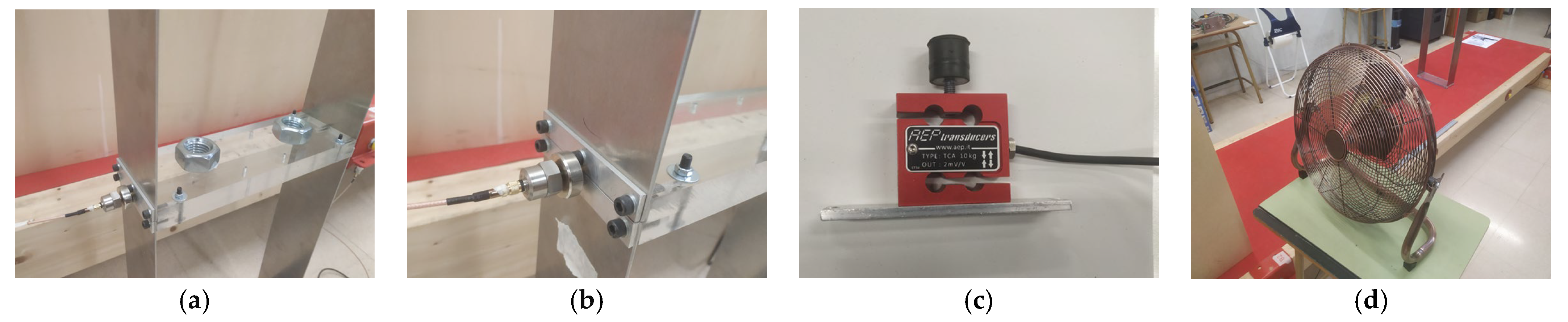
Regarding the experimental work, Figure 3 provides a detailed overview of the experimental equipment used in the study. M45 nuts weighing 190.5 g (Figure 3a) have been used to introduce discrete mass alterations at each floor of the building. The vibrational response of each floor was recorded using a set of four piezoelectric accelerometers, one per floor (Figure 3b). Finally, two different methods were employed to induce energy on the structure. First, a load cell (Figure 3c) was used to provide controlled input forces and identify the properties of the reference structure. Additionally, since SHM systems aim at detecting modifications and damage passively (i.e., without directly interacting with the structure), it is essential to assess the building’s ambient response. To simulate this, a fan (Figure 3d) was used to introduce random, uncontrolled forces, mimicking ambient excitation conditions.

3. Methodology

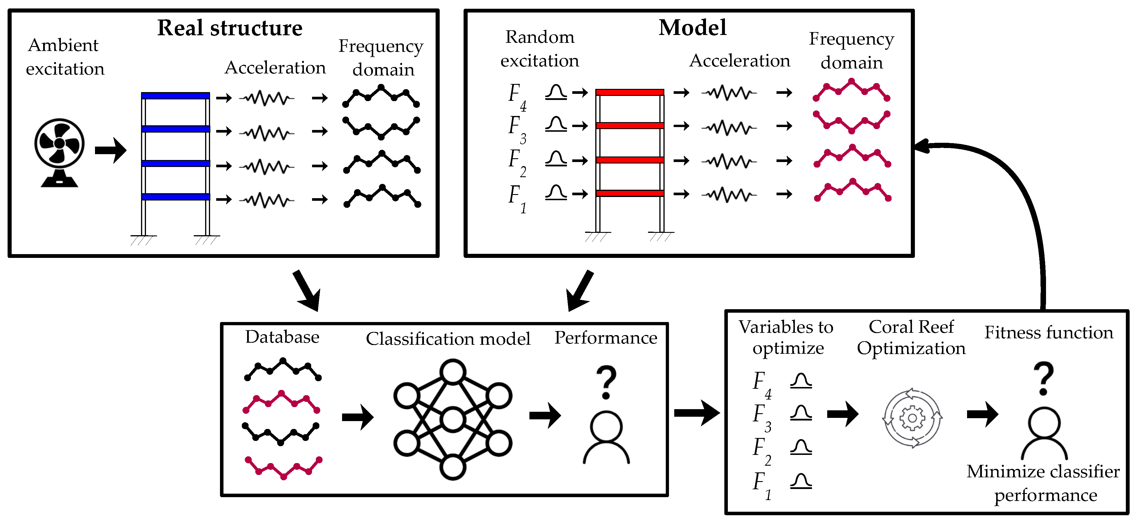
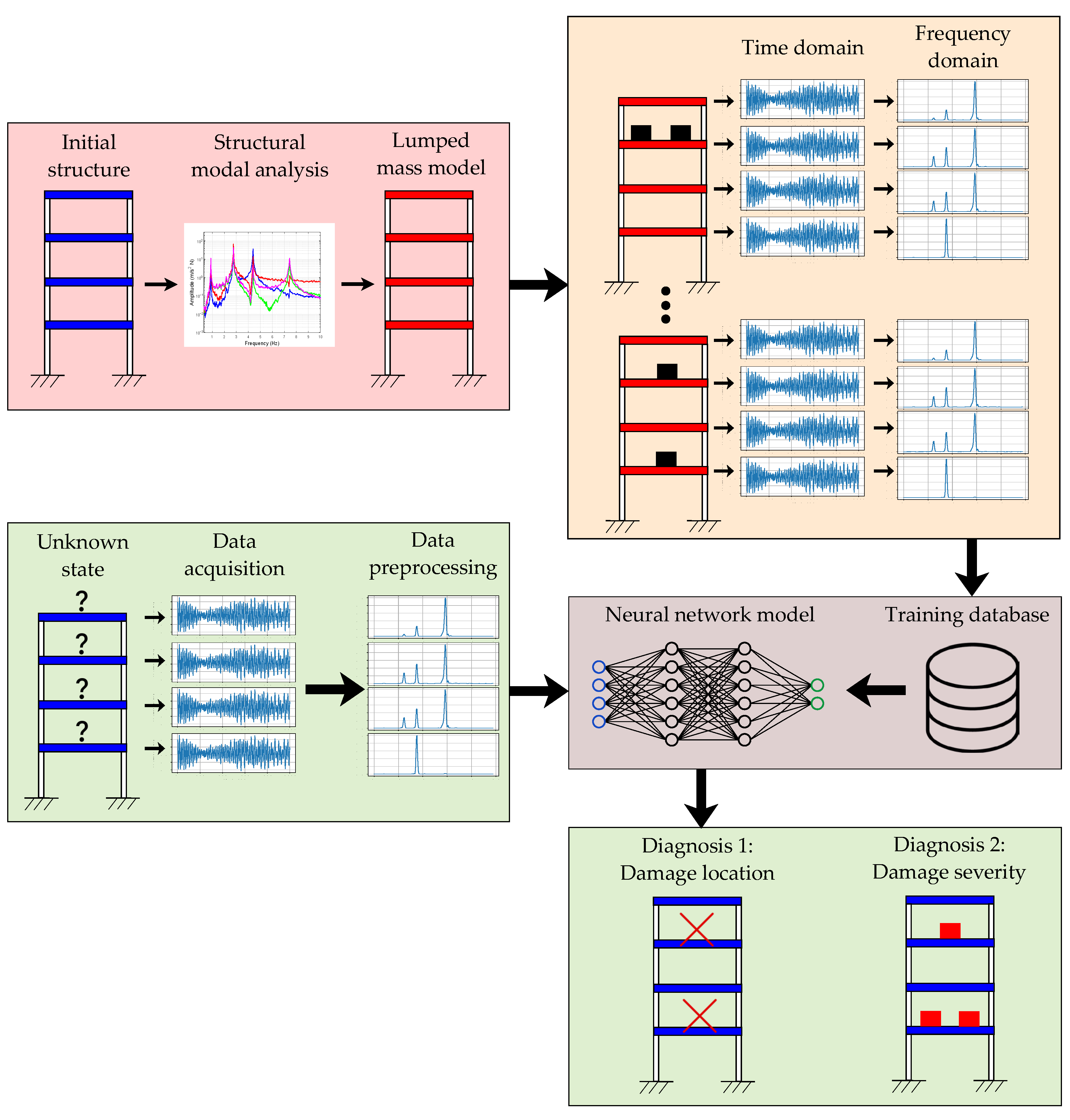
This section describes the proposed hybrid methodology for locating and estimating structural damage. Figure 4 provides an overview of the framework used in this work. This methodology can be divided into four different parts, which are represented by different colors in the figure and are detailed in the following subsections. Section 3.1 is devoted to the identification of the modal properties of the undamaged reference structure and the creation of the subsequent model. Then, once the model is created, different levels of simulated damage are defined, simulations are run, and data are processed in the frequency domain, labeled, and stored in a training database. This procedure is further detailed in Section 3.2. Afterwards, in Section 3.3, two architectures of neural network algorithms are defined and trained to locate and estimate the damage in the simulated structure, after a hyperparameter tuning process is performed. Finally, these neural models are validated with different levels of damage in the real structure (Section 3.4).

3.1. Structure Identification and Model Creation

The structure has been characterized both modally and physically: the modal analysis offers insights into its dynamic behavior, while the physical characterization enables the development of a reduced model for simulations.

The dynamic behavior of the reference structure is identified through an Experimental Modal Analysis (EMA), where the acceleration frequency response functions (FRFs), or accelerances, are measured and processed to estimate both the modal and the physical properties of the structure. An impact modal analysis technique has been used, where energy is induced in the structure using a load cell and its response is measured by a set of four piezoelectric accelerometers, one per floor. Synchronous data acquisition was carried out using a Dewesoft^® data acquisition system, with a sampling frequency of 400 Hz.

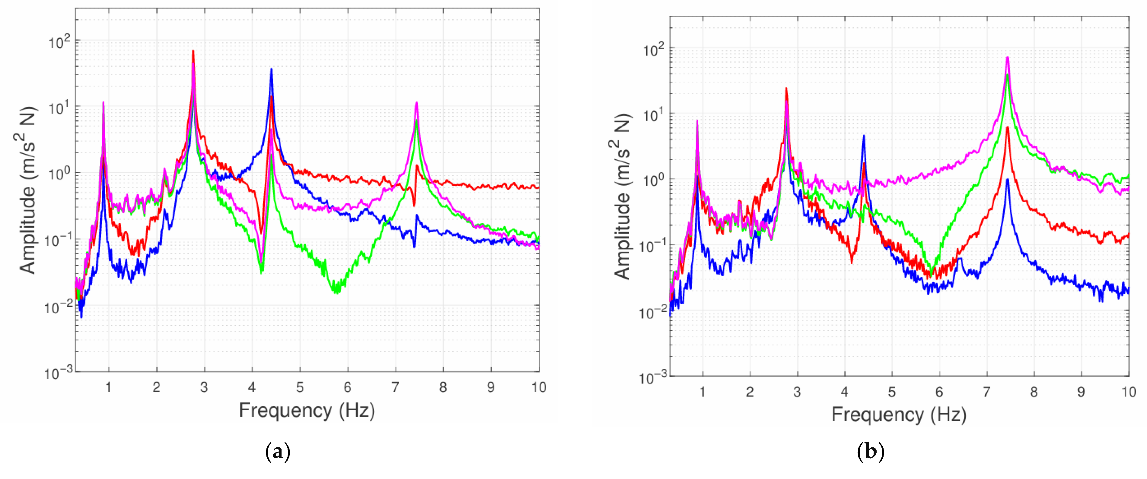
The registered data have been post-processed in order to estimate the experimental FRFs, considering a rectangular window with a size of 32,768 points. Figure 5 shows the measured FRFs, representing the system accelerance between 0 and 10 Hz. The natural frequencies of the reference structure, close to the accelerance peaks, are found at 0.89, 2.78, 4.39, and 7.45 Hz.

The physical parameters of the structure (mass, stiffness, and damping matrices) were obtained through a curve-fitting algorithm, aiming at minimizing the error between the experimental and analytical FRFs.

To determine the analytical accelerances of the system, its state-space representation was used (Equation (1)). In this model, the system input $f\left(t\right)$ represents a vector containing the forces applied to each floor of the structure, while the output $y\left(t\right)$ is a vector of the accelerations measured at each floor. The vector $x\left(t\right)$, composed of the state variables of the structure, is chosen to correspond to the position and velocity of each floor of the structure (Equation (2)).

$$\left\{\begin{array}{c}\dot{x}\left(t\right)=A_{S }x\left(t\right)+B_{S}f\left(t\right)\\ y\left(t\right)=C_{S}x\left(t\right)+D_{S}f\left(t\right)\end{array}\right.$$

(1)

$$x\left(t\right)=\left[\begin{array}{c}q\left(t\right)\\ \dot{q}\left(t\right)\end{array}\right] \mathrm{with} q\left(t\right)=\left[\begin{array}{c}\begin{array}{c}{x}_1\left(t\right)\\ x_2\left(t\right)\end{array}\\ \begin{array}{c}{x}_3\left(t\right)\\ x_4\left(t\right)\end{array}\end{array}\right]$$

(2)

The matrices $A_{S }$, $B_S$, $C_S$, and $D_S$ are selected to satisfy the structure’s equation of motion based on its physical properties (Equation (3)), where $M$, $C,$ and $K$ represent the mass, damping, and stiffness matrices, respectively (Equation (4)). Consequently, these matrices are defined as shown in the equations provided in Equation (5).

$$M\ddot{q}\left(t\right)+C\dot{q}\left(t\right)+Kq\left(t\right)=f\left(t\right)$$

(3)

$$\begin{gathered} M=\left[\begin{array}{cccc}{m}_1& & & \\ & m_2& & \\ & & m_3& \\ & & & m_4\end{array}\right] \\ K=\left[\begin{array}{cccc}{k}_1+k_2& {-k}_2& & \\ {-k}_2& k_2+k_3& {-k}_3& \\ & {-k}_3& k_3+k_4& {-k}_4\\ & & {-k}_4& k_4\end{array}\right] \\ C=\left[\begin{array}{cccc}{c}_1+c_2& {-c}_2& & \\ {-c}_2& c_2+c_3& {-c}_3& \\ & {-c}_3& c_3+c_4& {-c}_4\\ & & {-c}_4& c_4\end{array}\right] \end{gathered}$$

(4)

$$\begin{gathered} A_S=\left[\begin{array}{cc}0& I\\ {-M}^{-1}K& {-M}^{-1}C\end{array}\right]; B_S=\left[\begin{array}{c}0\\ M^{-1}\end{array}\right] \\ {C}_S=\left[\begin{array}{cc}{-M}^{-1}K& {-M}^{-1}C\end{array}\right]; D_S=M-1 \end{gathered}$$

(5)

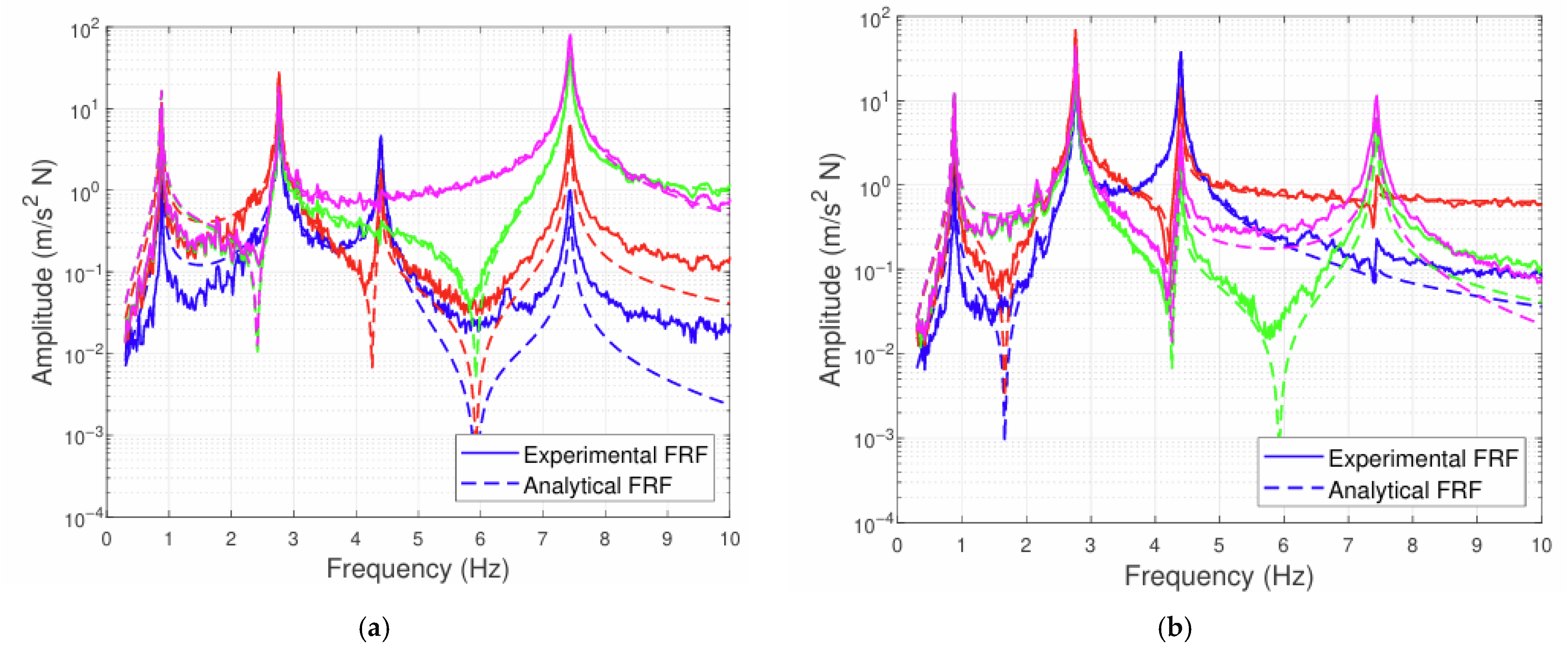
The physical parameters obtained after the curve-fitting process in order to fit the FRFs previously computed are presented in

Table 1. Optimized physical parameters.

Parameters	Values
$m_1$	1.27 kg
$m_2$	1.65 kg
$m_3$	1.94 kg
$m_4$	1.17 kg
$k_1$	643.5 N/m
$k_2$	796.5 N/m
$k_3$	321.4 N/m
$k_4$	310.7 N/m
$c_1$	0.500 Ns/m
$c_2$	0.005 Ns/m
$c_3$	0.094 Ns/m
$c_4$	0.000 Ns/m

for the reference structure (i.e., with no additional mass on any floor). Additionally, Figure 6 illustrates the comparison between the experimental (solid line) and analytical (dotted line) frequency response functions.

3.2. Generation of Training Database

Once the model is developed, it is used to simulate various levels of potential damage, generating a dataset for training the SDD models. First, the way of inducing energy into the structure is established, which represents a critical aspect of the proposed framework. One key advantage of this approach is its ability to classify experimentally measured scenarios without requiring prior experimental training data. Consequently, it is essential that the simulated vibrational data match the experimental data used to validate the system. Therefore, defining the method of excitation is vital, as the time-domain dynamic response can vary significantly depending on how the system is excited—whether through different locations, amplitudes, frequencies, or modes of excitation.

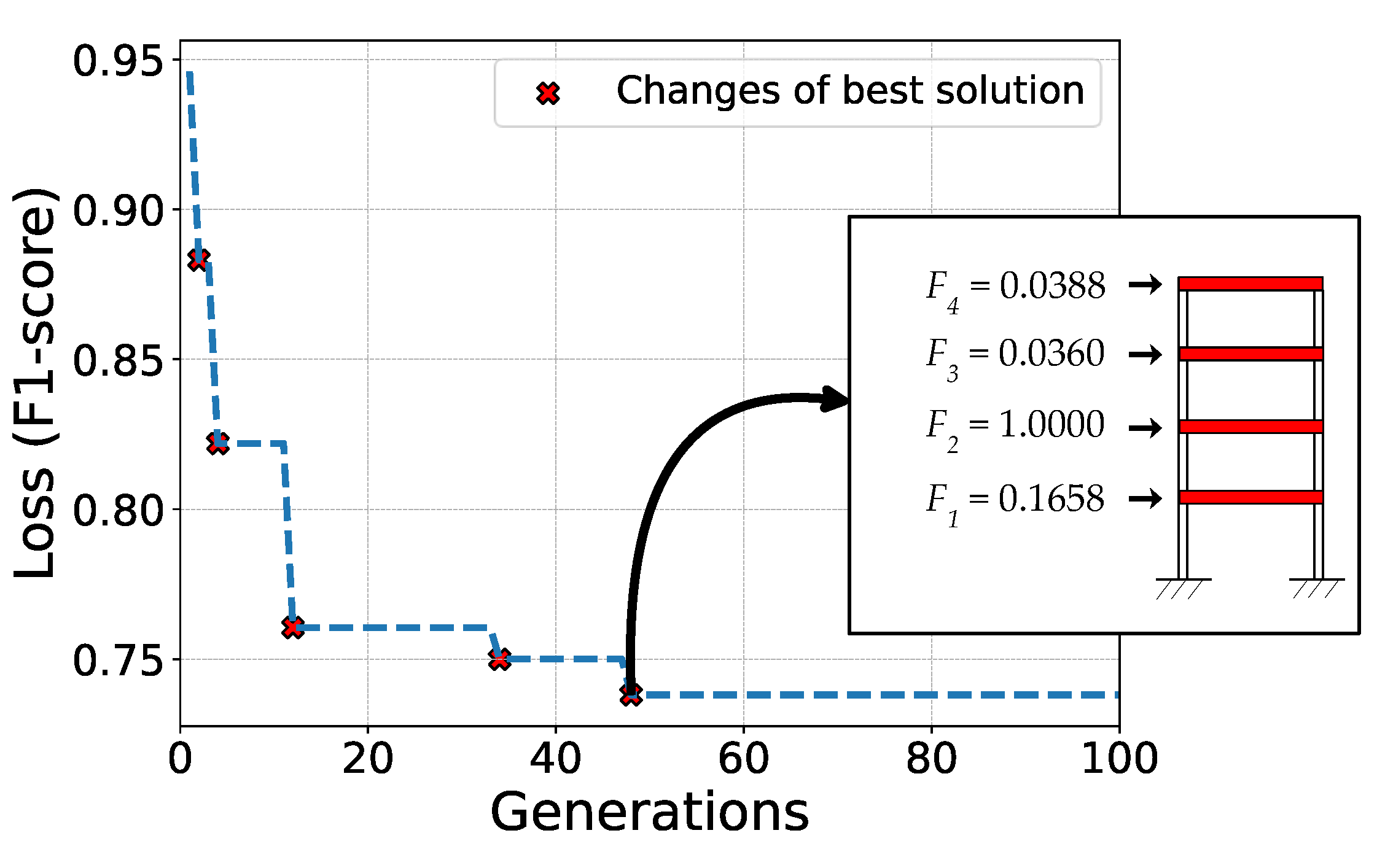
For this purpose, an evolutionary search was conducted to determine the optimal excitation parameters for the model, aiming to produce response levels as close as possible to those obtained experimentally. In experimental cases, the structure was excited using a device with sufficient energy and frequency content to ensure satisfactory results. Similarly, in the model, a random force with a normal distribution centered at 0 N was applied to each floor, with variance levels of $F_1$, $F_2$, $F_3$, and $F_{4 }$ for each of the floors, respectively. The search procedure for the optimal values of these parameters can be observed in Figure 7.

This approach is inspired by the concepts of Generative Adversarial Networks (GANs) [62], which combine a synthetic image generator with a discriminator that distinguishes between real and synthetic images. Through iterative training, both models progressively improve, enabling the generator to produce synthetic images that become increasingly realistic. The philosophy underlying this method aligns perfectly with the objectives of the proposed methodology, in which we aim to optimize the simulation parameters so that the resulting data closely resemble the experimental observations. The problem is addressed using a model to generate simulated data, paired with a neural network that acts as a discriminator to differentiate between real and simulated data. The input parameters of the model are optimized to increase the difficulty for the discriminator in distinguishing simulated data from real data.

A robust evolutionary optimization algorithm was employed: the Coral Reefs Optimization Algorithm with Substrate Layers (CRO-SL). The CRO-SL is a multi-method ensemble approach [63], based on the CRO algorithm [64]. In this multi-method approach, several search operators are applied to a single population, obtaining a powerful evolutionary-based method for optimization problems. The CRO-SL was initially introduced in [64], and the final multi-method ensemble, corresponding to the version used in this paper, was introduced in [65], where a probabilistic dynamic algorithm was proposed. This version of the CRO-SL is free-access, and a Python 3.10 code can be obtained via GitHub, as described in [65].

The fitness function consisted of the following:

• Creating a database with Fast Fourier Transforms (FFTs) belonging to the real undamaged structure and to the model. A 10 min experiment was performed in both cases. FFTs were obtained after slicing the signal into segments of varying lengths between 2 and 10 s. FFTs were computed on a domain between 0.2 and 10 Hz with a resolution of 25 points per Hz. After that, each FFT was normalized between 0 and 1, and the FFTs of each layer were concatenated into a single vector.
• Labeling the data (0 for simulated FFTs and 1 for real FFTs), shuffling the database, and splitting the data between train (80%) and test (20%).
• Training a simple neural network model for solving the binary classification task. The network consisted of three hidden layers with 128, 64, and 32 neurons, respectively, “relu” activation functions, the “adam” optimizer, and “binary crossentropy” as the loss function.
• The F1-score (Equation (6)) for the test data was returned as the fitness value. It is defined as the harmonic mean of precision ($p$, the ratio of correctly predicted positives to all predicted positives) and recall ($r$, the ratio of correctly predicted positives to all actual positives). This metric is widely used to evaluate the quality of binary classification predictions.

$$F_1={\displaystyle \frac{2 p r}{p+r}}$$

(6)

The optimization task was defined as a minimization problem; therefore, the objective is to find a set of input forces that produce FFTs as close as possible to those experimentally acquired, so that the performance of the neural classifier is as low as possible.

Finally, the different alterations of the physical properties in the undamaged structure model are defined so that the system is trained with all the potential scenarios. In the case studied, damage has been considered as discrete mass additions of 0.19 kg, ranging from zero to four masses added per floor. Sixteen possible combinations (24) of damage location have been considered, from the case with any floors damaged to the case with all floors damaged. For each of the 16 combinations, 50 cases of 2 min duration have been simulated, adding a random damage severity on each damaged floor, varying from 1 to 4 masses added. Therefore, a total of 800 simulations (16 combinations × 50 runs each) of 2 min duration have been executed.

The generated acceleration signals are then post-processed as follows:

• Each signal is divided into sets of $W_l$ points, containing information of $W_l$/1000 s, since the sampling frequency of the data acquisition system used to monitor the structure is 1000 Hz.
• Each set is transformed into the frequency domain by computing the FFT of these segments between 0.2 and 10 Hz (since the range of interest will be within these frequencies as observed in the identification of the reference structure). The resolution of these FFTs is parameterized with fr.
• Amplitudes of FFTs are normalized between 0 and 1. This normalization is performed independently for each segment. The FFT magnitudes are scaled by dividing them by the maximum amplitude within that same segment. This ensures that the normalization reflects the local spectral characteristics of each portion of the signal, avoiding biases that could arise from global amplitude differences across segments.
• A label is assigned to each FFT, corresponding to the damage level associated with that case. The codification of the labels consists of a single vector of 4 integer values, one for each floor, where 0 indicates the absence of damage and 1, 2, 3, and 4 correspond to the presence and severity of damage on that specific floor.

3.3. Neural Network Architecture Selection

This section describes the different neural architectures used for conducting the supervised learning task of SDD. Two different tasks are defined, representing the two different diagnoses of the SHM application: The first one consists of identifying and locating structural damage, regardless of the damage severity. The second one represents the estimation of the damage severity of each floor of the structure.

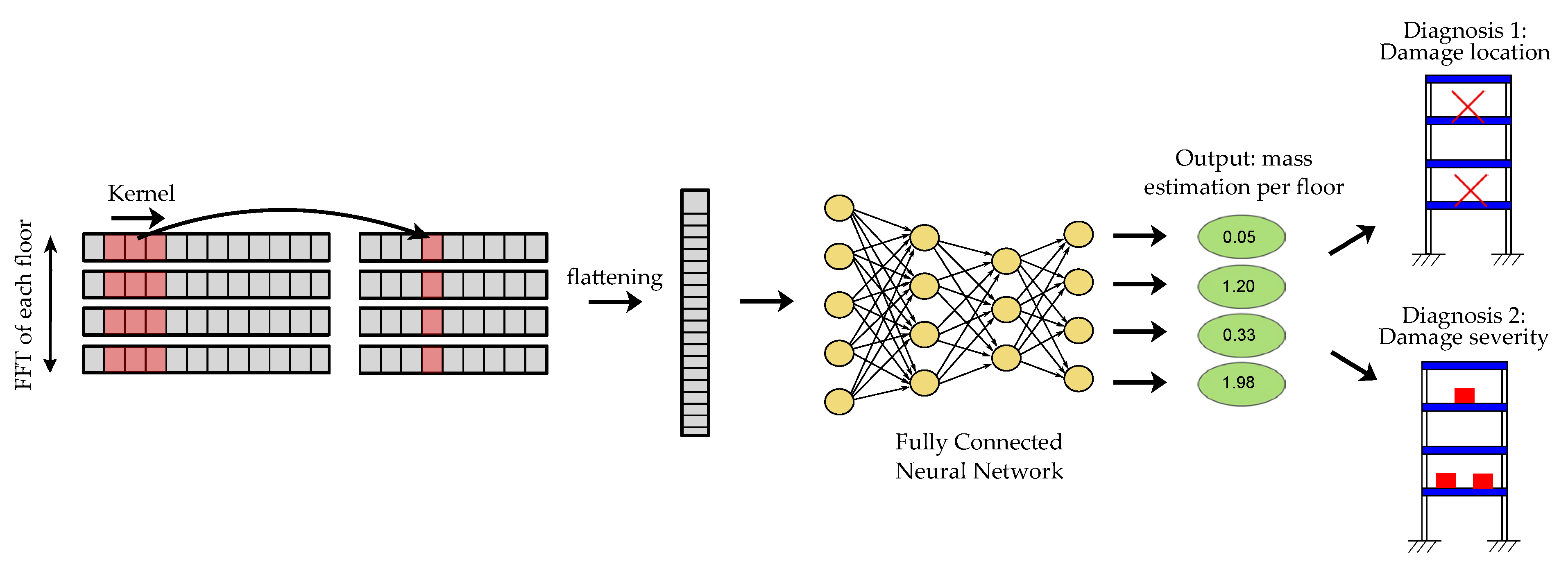
In both frameworks, a single-task neural network is considered. The model is trained to solve a multi-output regression problem, where each output corresponds to the damage severity estimation of each floor. This output is then post-processed to assess for the two diagnoses, by assigning a value of 1 if ${\widehat{y}}_i$ ≥ 0.5 or 0 if ${\widehat{y}}_i$ < 0.5 in the case of damage location, or by rounding to the nearest integer in the case of damage severity. Two different architectures of neural networks have been considered: a Fully Connected Neural Networks (FCNNs) [66] and a 1D-CNN [16].

FCNN refers to a neural network architecture composed of multiple layers: an input layer, one or more hidden layers, and one output layer. Each layer is composed of units called nodes or neurons which are connected to every other node in the neighboring layers by means of weighted links.

Convolutional Neural Networks (CNNs) [16] are a specific type of feedforward neural networks initially developed for tasks related to image processing and computer vision. Convolution layers are responsible for learning the features from input data. They apply and slide a filter over the data. This filter, also known as a kernel, contains learnable weights and biases, and is the equivalent of nodes in a regular neural network layer.

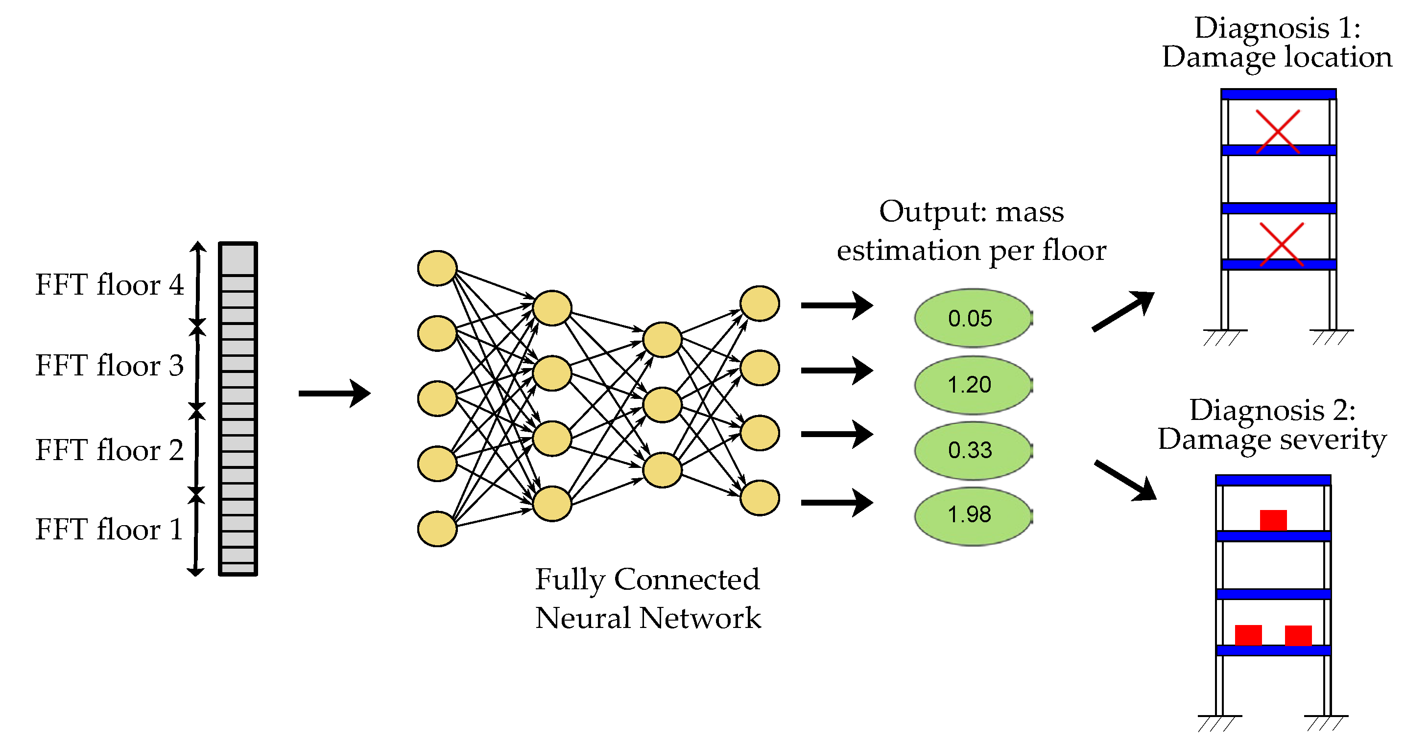
The architecture of both types of neural networks Is depicted In Figure 8 and Figure 9, considering the FCNN and the 1D-CNN architectures, respectively. The main difference resides in the way the data is fed into the network. In the case of the 1D-CNN network, the FFTs of each floor are introduced independently, so that a one-dimensional kernel runs through each of the signals and extracts their main characteristics. This is repeated over a number of layers and with a number of filters per layer (parameters which are determined by a random hyperparameter search). Subsequently, the extracted features are grouped into a single vector and fed to an FCNN. In the case of the FCNN, the FFTs of each floor are concatenated into a single vector, which constitutes the input layer of the neural network. Similarly, the number of layers and neurons per layer is determined by means of a random hyperparameter search, which is detailed below.

3.4. Diagnosis of Real Structure

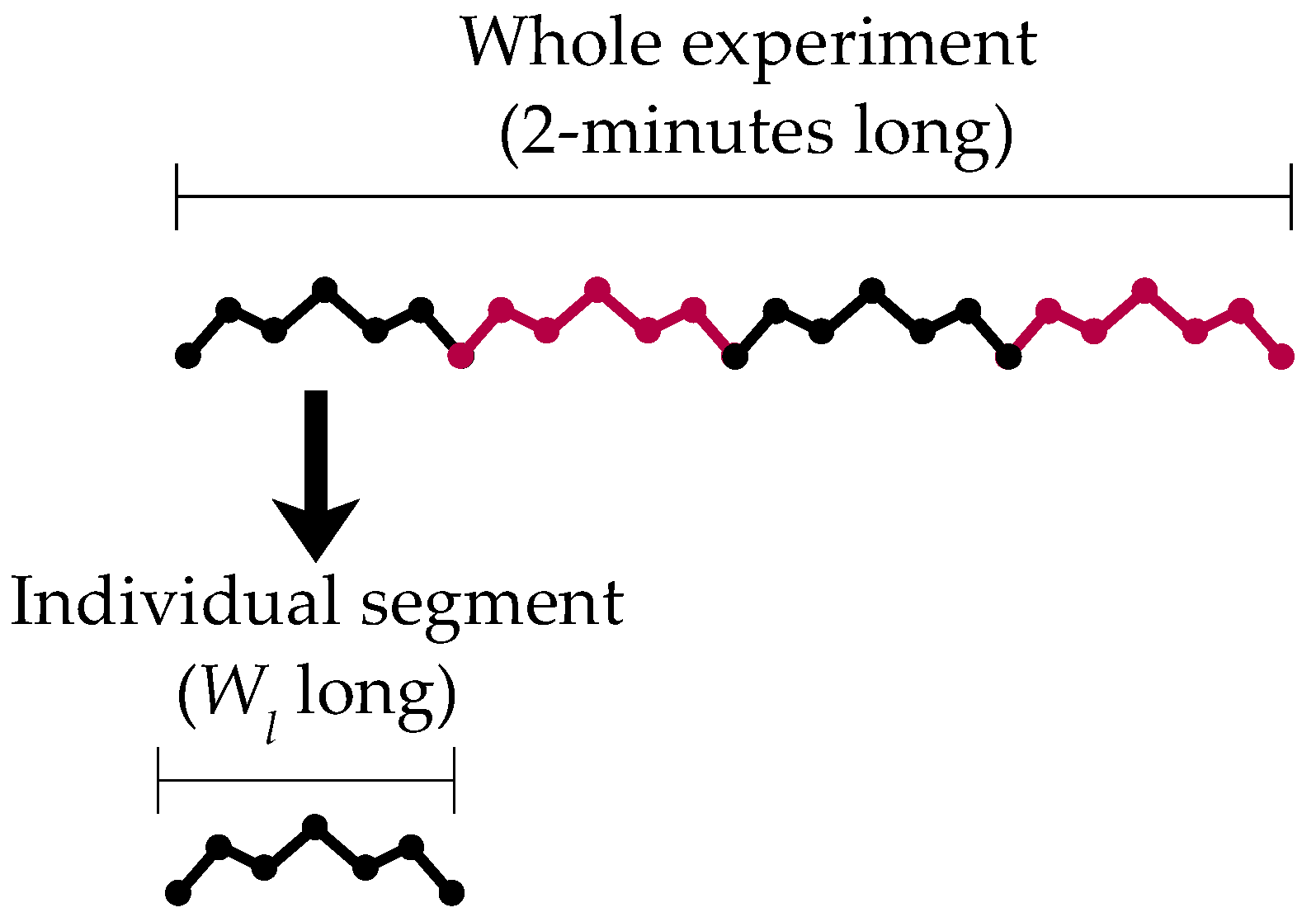
Finally, the network outputs are processed to obtain a diagnosis of the structure’s condition by averaging the outputs for each segment corresponding to the same scenario. For each scenario studied, a 2 min time signal is acquired at a sampling frequency of 1000 Hz, resulting in 120,000 data points. This signal is divided into segments of $W_l$ points, which are then input into the neural network models, yielding a total of 120,000/$W_l$ outputs for each structural condition. Various values of $W_l$ have been considered. Therefore, the diagnosis for a particular scenario is derived by averaging the outputs of each segment. The advantages of segmentation techniques can be found in [67].

4. Results

This section describes the experimental work performed. In the first place, Section 4.1 shows the optimization results for obtaining the optimal excitation levels in the model. Then, Section 4.2 describes the hyperparameter tuning procedure and its results. Finally, Section 4.3 provides the SDD experimental results.

4.1. Diagnosis of Real Structure

The optimal excitation levels for inducing energy into the model were determined after an optimization procedure was run. Random forces with a normal distribution centered at 0 N were applied to each floor, considering variance levels of $F_1$, $F_2$, $F_3$, and $F_4$, respectively. The limits of these variances were set at 0 and 1. The CRO-SL is a multi-method ensemble approach, where several operators are applied to a single population. Four different operators have been employed in this optimization process: BLX-α crossover [68], Differential Evolution [69], Multipoint Crossover [70], and Harmony Search [71]. The population size has been set at 100 individuals, and the algorithm has been run for 100 generations.

Figure 10 shows the results provided by the CRO-SL optimization algorithm, where the evolution of the fitness value is observed throughout the different generations. A decrease in the classification performance is observed from an F1-score of nearly 0.95 to an F1-score below 0.75. The variances provided by the best solution are the ones indicated in the figure, corresponding to 0.1658, 1, 0.036, and 0.0388 for floors 1, 2, 3, and 4, respectively.

4.2. Hyperparameters Considered

This section describes the procedure followed to determine the optimal combination of hyperparameters for each model.

First, 16 damage location cases are defined, ranging from [0, 0, 0, 0] to [1, 1, 1, 1], where a value of 1 indicates the presence of damage on a specific floor. For each case, 50 simulations of 2 min duration are generated, with random damage severity affecting between one and four masses. The input forces used in the simulations are derived from those obtained in Section 4.1.

The list of hyperparameters considered are detailed in

Table 2. Hyperparameters considered (in bold the selected ones).

	Hyperparameter	Potential Values
FCNN architecture	Window length (Wl)	[2000, 3000, 4000, 5000, 6000, 8000, 10,000]
	FFT sample frequency	[10, 20, 30, 40, 50]
	Activation function	[relu, sigmoid]
	Patience	[10, 20, 30, … 120, … 180, 190, 200]
	Loss function	[mae, mse]
	N° of hidden layers	[1, 2, 3, 4, 5, 6]
	Window length (Wl)	[2000, 3000, 4000, 5000, 6000, 8000, 10,000]
1D-CNN architecture	FFT sample frequency	[10, 20, 30, 40, 50]
	Activation function	[relu, sigmoid]
	Patience	[10, 20, 30, … 130, … 180, 190, 200]
	Loss function	[mae, mse]
	# of hidden layers in FCNN	[1, 2, 3, 4]
	# of convolutional layers	[1, 2, 3, 4, 5, 6]
	Kernel size	[2, 3, 4, 5, 6, 7, 8, 9, 10]

for both neural network architectures. These variables contain both processing parameters ($W_l$ and FFT sample frequency), and neural model parameters.

A random search consisting of 100 hyperparameter combinations is conducted for each framework. In each iteration, the dataset is processed using the selected parameters, shuffled, and split into training (70%), test (15%), and validation (15%) sets. The training data is used to fit the model, while the validation set guides hyperparameter tuning and early stopping. Finally, the test set is reserved for evaluating the model’s performance on unseen data, ensuring the generalizability of the results.

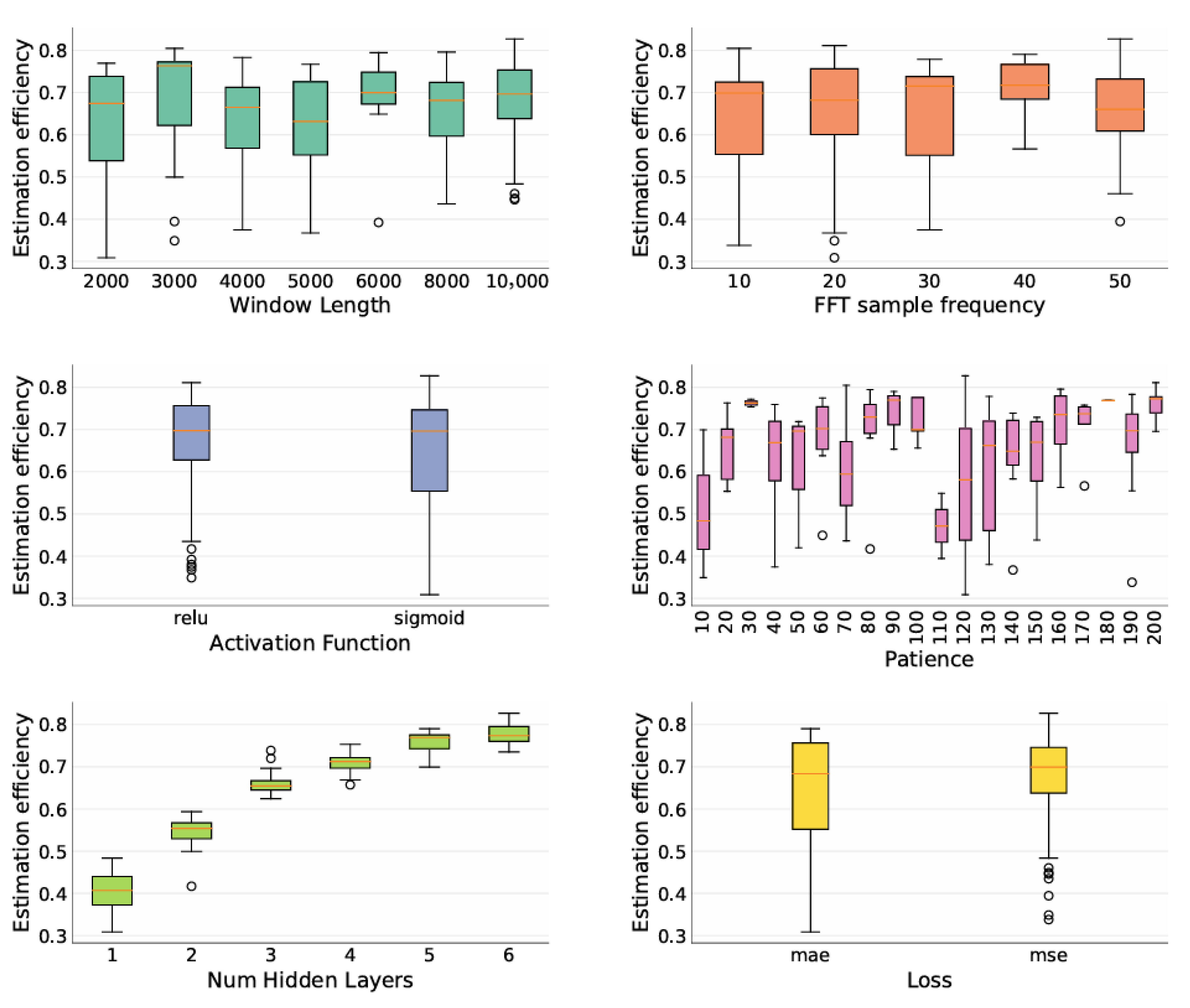
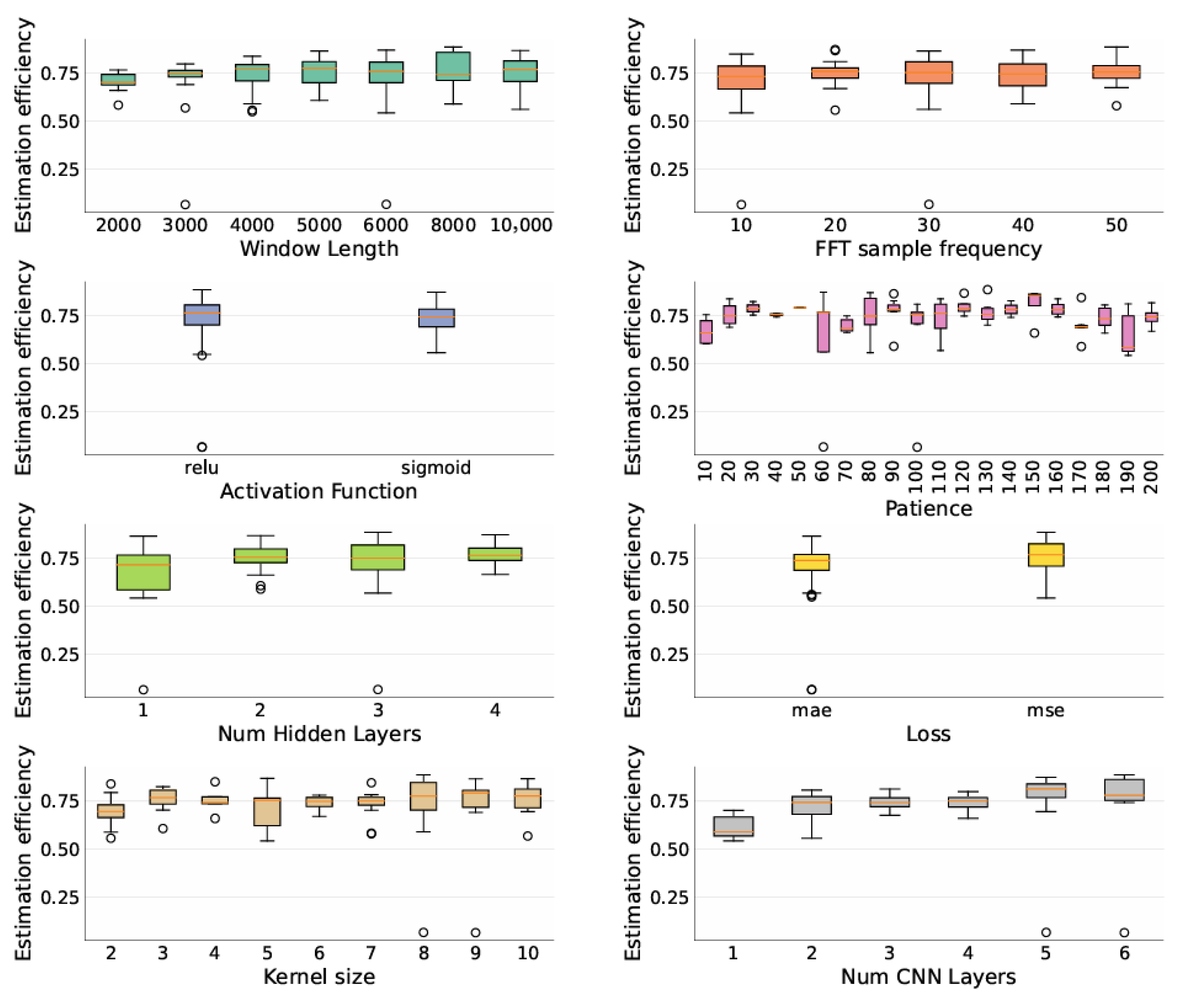
The optimal combination of hyperparameters is selected based on the criterion of estimation efficiency for damage severity. A test case is deemed successful if the damage in all floors is accurately located and quantified. A value of 1 in the estimation efficiency metric indicates that all the test samples are estimated correctly. Figure 11 and Figure 12 show the influence of each parameter on the test error metric for the FCNN and 1D-CNN cases, respectively, showing that the most critical parameters are the number of hidden layers on the FCNN architecture and the number of CNN layers in the 1D-CNN architecture, indicating that a more complex architecture yields better estimation results in both cases. The optimal set of parameters for both architectures is highlighted in bold in Table 2.

4.3. Experimental Results

This section shows the results obtained for the experimental validation process. Fifty-one experiments of 2 min duration were recorded, considering different states of damage location and severity (

Table 3. Experimental damage cases considered.

Exp Number	Damage State	Exp Number	Damage State	Exp Number	Damage State
1	[0 0 0 0]	1	[0 0 3 0]	1	[0 0 1 2]
2	[1 0 0 0]	2	[0 0 0 3]	2	[4 0 0 0]
3	[0 1 0 0]	3	[1 1 1 0]	3	[0 4 0 0]
4	[0 0 1 0]	4	[1 1 0 1]	4	[0 0 4 0]
5	[0 0 0 1]	5	[1 0 1 1]	5	[0 0 0 4]
6	[2 0 0 0]	6	[0 1 1 1]	6	[3 1 0 0]
7	[0 2 0 0]	7	[2 1 0 0]	7	[3 0 1 0]
8	[0 0 2 0]	8	[2 0 1 0]	8	[3 0 0 1]
9	[0 0 0 2]	9	[2 0 0 1]	9	[1 3 0 0]
10	[1 1 0 0]	10	[1 2 0 0]	10	[0 3 1 0]
11	[0 1 1 0]	11	[0 2 1 0]	11	[0 3 0 1]
12	[0 0 1 1]	12	[0 2 0 1]	12	[1 0 3 0]
13	[1 0 1 0]	13	[1 0 2 0]	13	[0 1 3 0]
14	[1 0 0 1]	14	[0 1 2 0]	14	[0 0 3 1]
15	[0 1 0 1]	15	[0 0 2 1]	15	[1 0 0 3]
16	[3 0 0 0]	16	[1 0 0 2]	16	[0 1 0 3]
17	[0 3 0 0]	17	[0 1 0 2]	17	[0 0 1 3]

). As mentioned in Section 3.2, the structure was excited using a small fan (Figure 3d), simulating environmental excitation due to the action of the wind.

Then, once the optimal set of hyperparameters is obtained for each architecture, training data is generated considering 50 simulations of 2 min duration for each of the 16 potential damage location states, with random damage severity between one and four masses, and considering the input forces obtained by simulation in Section 4.1. Subsequently, the neural network models are created and trained with the corresponding parameters, and the experimental SDD performance is assessed. For each task (damage location and severity estimation), two error metrics are considered: one indicating the efficiency of the network to assess the damage state of each individual time segment (of $W_l$ length), and the other indicating the diagnosis of the particular scenario by averaging the outputs of each segment (as discussed in Section 3.4) (Figure 13). In both metrics, the performance is measured as the efficiency $\epsilon$ (Equation (7)), where $C$ stands for the number of correct diagnosis and $T$ stands for the total number of cases. A correct diagnosis is considered only when all the floor states are correctly identified.

$$\epsilon \left(\%\right)=100 {\displaystyle \frac{C}{T}}$$

(7)

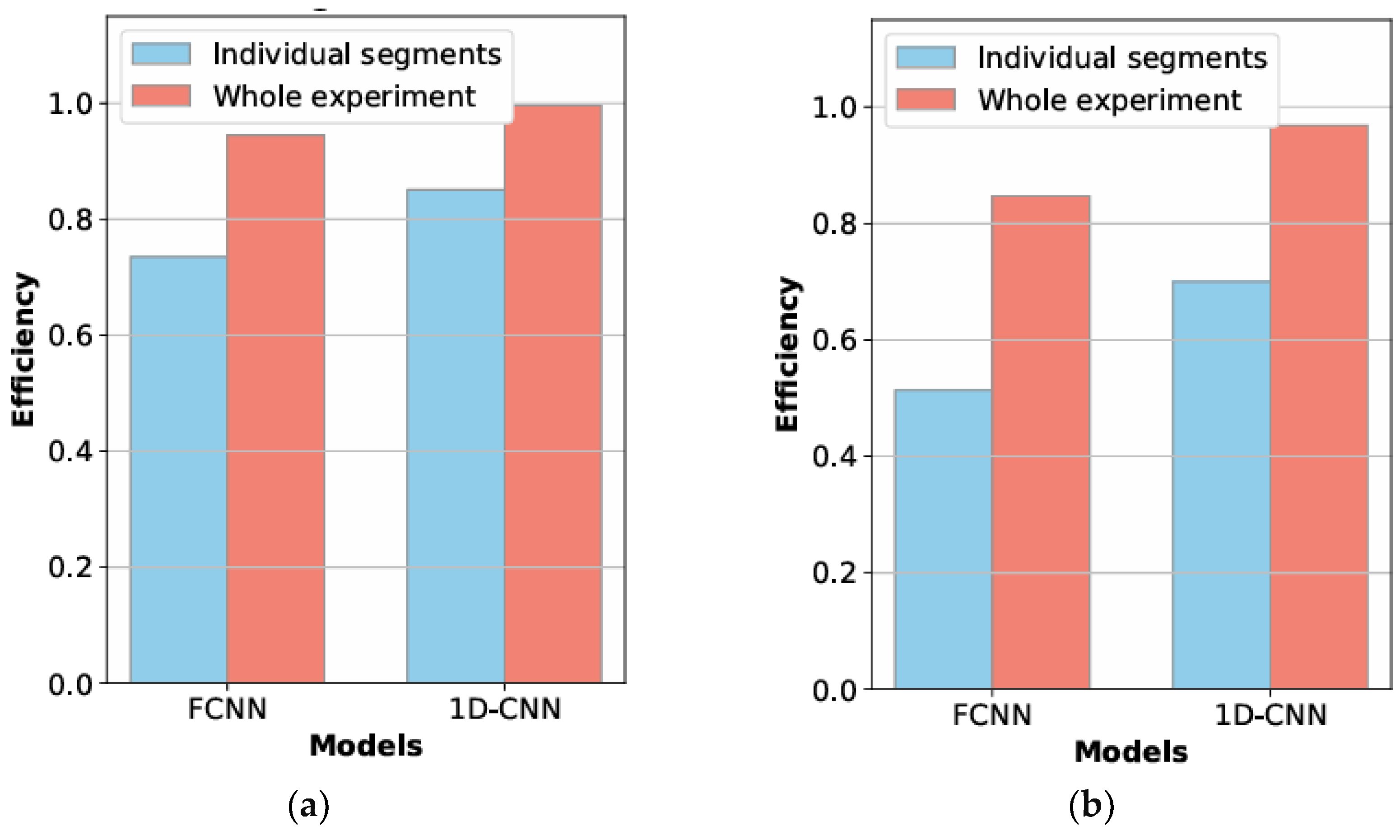
In order to account for the inherent stochastic variability present in both the generation of training data and the training process of the neural network, each model (FCNN and 1D-CNN) is trained five times with different training data. The performance results obtained after all the training runs are shown in

Table 4. Performance results of both neural architectures assessed and for the five different training runs to account for stochastic variability.

	Damage Location		Severity Estimation
	Ind. Segments	Whole Experiment	Ind. Segments	Whole Experiment
FCNN (training run 1)	0.7598	0.9804	0.5106	0.8235
FCNN (training run 2)	0.7230	0.9216	0.5294	0.8824
FCNN (training run 3)	0.7100	0.9020	0.4951	0.8039
FCNN (training run 4)	0.7600	0.9410	0.5250	0.8040
FCNN (training run 5)	0.7230	0.9800	0.5070	0.9220
FCNN (ave ± std)	0.7351 ± 0.0231	0.9451 ± 0.0351	0.5136 ± 0.0139	0.8471 ± 0.0526
1D-CNN (training run 1)	0.8719	1.0000	0.7085	0.9804
1D-CNN (training run 2)	0.8418	1.0000	0.7242	1.0000
1D-CNN (training run 3)	0.8405	1.0000	0.6797	0.9608
1D-CNN (training run 4)	0.8710	0.9800	0.7370	0.9610
1D-CNN (training run 5)	0.8290	1.0000	0.6500	0.9410
1D-CNN (ave ± std)	0.8507 ± 0.0194	0.9961 ± 0.0088	0.6999 ± 0.0353	0.9686 ± 0.0223

. The results obtained demonstrate satisfactory performance in both architectures; however, a significant improvement is evident when using the 1D-CNN framework. In terms of damage localization, the FCNN achieves accuracy rates of approximately 95%, while the 1D-CNN reaches nearly 100%. Additionally, for damage severity estimation, accuracy increases from an average of 85% with the FCNN to 97% with the convolutional network.

It is also possible to observe how, while there is room for improvement when detecting damage in individual segments (10 s in the case of the FCNN framework and 8 s in the case of 1D-CNN) efficiency rates are 74% and 85% in the case of damage location, and 51% and 70% in the case of severity estimation. When diagnosing the structure by averaging over the 2 min duration of each experiment, the results become practically perfect in both tasks.

Figure 14 compares the performance of the FCNN framework over the 1D-CNN framework, demonstrating the superiority of the latter in all cases. It can be concluded that using FFTs as input data is more effectively handled by a convolutional network, as this approach preserves the sequential nature of the data.

5. Conclusions

Hybrid approaches in SDD overcome the limitations of purely data-driven or model-based methods. Data-driven techniques require large datasets that are often unavailable, while model-based methods struggle with real-world variability and complexity. The hybridization not only improves detection accuracy but also ensures a more practical and scalable solution for SHM applications.

In this study, the proposed hybrid methodology demonstrated the effectiveness of combining model-generated training data with neural network-based classification for locating and assessing the damage in a real lab-scale structure. In this process, the following two critical elements are essential: the modal identification of the structure, in order to obtain an accurate model, and the identification of its operating conditions, to account for the possible ways of inducing energy in the model so that the simulated behavior closely resembles that of the real structure. The results show that the integration of neural-based computational learning techniques, fed with frequency-domain information from 8 s duration segments, achieves near-perfect efficiency rates in both damage localization and severity estimation (99.61% and 96.86%, respectively) when diagnosing the damage states of the 51 experimental cases of 2 min duration considered. It was also observed that convolutional networks, which effectively preserve the sequential nature of input data such as FFTs, offer superior performance compared to other architectures such as Fully Connected Neural Networks (FCNNs).

The proposed approach provides the following contributions to the field of Structural Damage Detection (SDD): First, it is capable of detecting damage in a structure, accurately locating the damaged areas and predicting their severity. This capability has been successfully demonstrated and experimentally implemented on a laboratory-scale structure. Second, the method enables the diagnosis of a structural state without requiring complex processing of the measured data, relying solely on the computation of FFTs from 8 s duration segments. Finally, it overcomes one of the main challenges of supervised Structural Health Monitoring (SHM) approaches (namely, the need for training data from both undamaged and damaged structures), by employing training data generated through model-based simulations. However, the main limitation of the proposed approach lies in the detection of different types of damage, which, for the moment, is restricted to detect mass changes.

Future directions for this research are as follows: (1) enhancing the capability to detect the location and severity of various types of damage, including the discrimination between changes in mass and stiffness, and accurately predicting the severity of each type; (2) extending the methodology to more complex structures, where the model must be capable of locating damage within a continuous domain; and (3) implementing the methodology on hardware systems to enable near-real-time damage detection.

References

1. Frangopol, D.M.; Brühwiler, E.; Faber, M.H.; Adey, B. Life-cycle performance of deteriorating structures. Struct. Eng. Int. 2003, 13, 202–204. [Google Scholar] [CrossRef] [Scilit]
2. Stache, M.; Guettler, M.; Marburg, S. A precise non-destructive damage identification technique of long and slender structures based on modal data. J. Sound Vib. 2016, 365, 89–101. [Google Scholar] [CrossRef] [Scilit]
3. Cosenza, E.; Manfredi, G. Damage indices and damage measures. Prog. Struct. Eng. Mater. 2000, 2, 50–59. [Google Scholar] [CrossRef]
4. Agdas, D.; Rice, J.A.; Martinez, J.R.; Lasa, I.R. Comparison of visual inspection and structural-health monitoring as bridge condition assessment methods. J. Perform. Constr. Facil. 2016, 30, 04015049. [Google Scholar] [CrossRef] [Scilit]
5. Cha, Y.-J.; Buyukozturk, O. Structural damage detection using modal strain energy and hybrid multiobjective optimization. Comput.-Aided Civ. Infrastruct. Eng. 2015, 30, 347–358. [Google Scholar] [CrossRef] [Scilit]
6. Farrar, C.R.; Worden, K. An introduction to structural health monitoring. Philos. Trans. R. Soc. A Math. Phys. Eng. Sci. 2007, 365, 303–315. [Google Scholar] [CrossRef] [Scilit]
7. Avci, O.; Abdeljaber, O.; Kiranyaz, S.; Hussein, M.; Gabbouj, M.; Inman, D.J. A review of vibration-based damage detection in civil structures: From traditional methods to machine learning and deep learning applications. Mech. Syst. Signal Process. 2021, 147, 107077. [Google Scholar] [CrossRef] [Scilit]
8. Wahab, M.A.; De Roeck, G. Damage detection in bridges using modal curvatures: Application to a real damage scenario. J. Sound Vib. 1999, 226, 217–235. [Google Scholar] [CrossRef] [Scilit]
9. Diez, A.; Khoa, N.L.D.; Alamdari, M.M.; Wang, Y.; Chen, F.; Runcie, P. A clustering approach for structural health monitoring on bridges. J. Civ. Struct. Health Monit. 2016, 6, 429–445. [Google Scholar] [CrossRef] [Scilit]
10. Farrar, C.R.; Doebling, S.W.; Nix, D.A. Vibration–based structural damage identification. Philos. Trans. R. Soc. London. Ser. A Math. Phys. Eng. Sci. 2001, 359, 131–149. [Google Scholar] [CrossRef] [Scilit]
11. Chesné, S.; Deraemaeker, A. Damage localization using transmissibility functions: A critical review. Mech. Syst. Signal Process. 2013, 38, 569–584. [Google Scholar] [CrossRef] [Scilit]
12. Amezquita-Sanchez, J.P.; Adeli, H. Signal processing techniques for vibration-based health monitoring of smart structures. Arch. Comput. Methods Eng. 2016, 23, 1–15. [Google Scholar] [CrossRef] [Scilit]
13. Montalvao, D.; Maia, N.M.M.; Ribeiro, A.M.R. A review of vibration based structural health monitoring with special emphasis on composite materials. Shock Vib. Dig. 2006, 38, 295–324. [Google Scholar] [CrossRef] [Scilit]
14. Das, S.; Saha, P.; Patro, S. Vibration-based damage detection techniques used for health monitoring of structures: A review. J. Civ. Struct. Health Monit. 2016, 6, 477–507. [Google Scholar] [CrossRef] [Scilit]
15. Cruz, P.J.; Salgado, R. Performance of vibration-based damage detection methods in bridges. Comput.-Aided Civ. Infrastruct. Eng. 2009, 24, 62–79. [Google Scholar] [CrossRef] [Scilit]
16. Abdeljaber, O.; Avci, O.; Kiranyaz, S.; Gabbouj, M.; Inman, D.J. Realtime vibration-based structural damage detection using one-dimensional convolutional neural networks. J. Sound Vib. 2017, 388, 154–170. [Google Scholar] [CrossRef] [Scilit]
17. Fugate, M.L.; Sohn, H.; Farrar, C.R. Vibration-based damage detection using statistical process control. Mech. Syst. Signal Process. 2001, 15, 707–721. [Google Scholar] [CrossRef] [Scilit]
18. Magalhães, F.; Cunha, A.; Caetano, E. Vibration based structural health monitoring of an arch bridge: From automated oma to damage detection. Mech. Syst. Signal Process. 2012, 28, 212–228. [Google Scholar] [CrossRef] [Scilit]
19. Fritzen, C.P. Vibration-based structural health monitoring–concepts and applications. Key Eng. Mater. 2005, 293, 3–20. [Google Scholar] [CrossRef] [Scilit]
20. Fassois, S.D.; Kopsaftopoulos, F.P. Statistical Time Series Methods for Vibration Based Structural Health Monitoring; Springer: Berlin/Heidelberg, Germany, 2013. [Google Scholar]
21. Deraemaeker, A.; Reynders, E.; De Roeck, G.; Kullaa, J. Vibration-based structural health monitoring using output-only measurements under changing environment. Mech. Syst. Signal Process. 2008, 22, 34–56. [Google Scholar] [CrossRef] [Scilit]
22. Shadan, F.; Khoshnoudian, F.; Esfandiari, A. A frequency response-based structural damage identification using model updating method. Struct. Control Health Monit. 2016, 23, 286–302. [Google Scholar] [CrossRef] [Scilit]
23. Yang, Y.; Zhang, Y.; Tan, X. Review on vibration-based structural health monitoring techniques and technical codes. Symmetry 2021, 13, 1998. [Google Scholar] [CrossRef] [Scilit]
24. Moallemi, A.; Burrello, A.; Brunelli, D.; Benini, L. Model-based vs. data driven approaches for anomaly detection in structural health monitoring: A case study. In Proceedings of the 2021 IEEE International Instrumentation and Measurement Technology Conference (I2MTC), Glasgow, UK, 17–20 May 2021; pp. 1–6. [Google Scholar]
25. Nagayama, T.; Spencer, B.; Agha, G.; Mechitov, K. Model-based data aggregation for structural monitoring employing smart sensors. In Proceedings of the Third International Conference on Networked Sensing Systems, Rosemont, IL, USA, 31 May–2 June 2006; pp. 1–8. [Google Scholar]
26. Avendano-Valencia, L.D.; Fassois, S.D. Gaussian mixture random coefficient model based framework for shm in structures with time–dependent dynamics under uncertainty. Mech. Syst. Signal Process. 2017, 97, 59–83. [Google Scholar] [CrossRef] [Scilit]
27. Biliszczuk, J.; Hawryszków, P.; Teichgraeber, M. Shm system and a fem model-based force analysis assessment in stay cables. Sensors 2021, 21, 1927. [Google Scholar] [CrossRef] [Scilit]
28. Moriot, J.; Quaegebeur, N.; Le Duff, A.; Masson, P. A model-based approach for statistical assessment of detection and localization performance of guided wave–based imaging techniques. Struct. Health Monit. 2018, 17, 1460–1472. [Google Scholar] [CrossRef] [Scilit]
29. Qiu, L.; Fang, F.; Yuan, S.; Boller, C.; Ren, Y. An enhanced dynamic gaussian mixture model–based damage monitoring method of aircraft structures under environmental and operational conditions. Struct. Health Monit. 2019, 18, 524–545. [Google Scholar] [CrossRef] [Scilit]
30. Chen, Q.; Cao, J.; Zhu, S. Data-driven monitoring and predictive maintenance for engineering structures: Technologies. implementation challenges, and future directions. IEEE Internet Things J. 2023, 10, 14527–14551. [Google Scholar] [CrossRef] [Scilit]
31. Eltouny, K.; Gomaa, M.; Liang, X. Unsupervised learning methods for data-driven vibration-based structural health monitoring: A review. Sensors 2023, 23, 3290. [Google Scholar] [CrossRef] [Scilit]
32. Niyirora, R.; Ji, W.; Masengesho, E.; Munyaneza, J.; Niyonyungu, F.; Nyirandayisabye, R. Intelligent damage diagnosis in bridges using vibration-based monitoring approaches and machine learning: A systematic review. Results Eng. 2022, 16, 100761. [Google Scholar] [CrossRef] [Scilit]
33. Höll, S.; Humer, C. Deep predictions and transfer learning for simulation driven structural health monitoring based on guided waves. Expert Syst. Appl. 2024, 238, 122133. [Google Scholar] [CrossRef] [Scilit]
34. Rodrigues, M.; Miguéis, V.L.; Felix, C.; Rodrigues, C. Machine learning and cointegration for structural health monitoring of a model under environmental effects. Expert Syst. Appl. 2024, 238, 121739. [Google Scholar] [CrossRef] [Scilit]
35. Flah, M.; Nunez, I.; Chaabene, W.B.; Nehdi, M.L. Machine learning algorithms in civil structural health monitoring: A systematic review. Arch. Comput. Methods Eng. 2021, 28, 2621–2643. [Google Scholar] [CrossRef] [Scilit]
36. Bao, Y.; Li, H. Machine learning paradigm for structural health monitoring. Struct. Health Monit. 2021, 20, 1353–1372. [Google Scholar] [CrossRef]
37. Gardner, P.; Barthorpe, R.; Lord, C. The Development of a Damage Model for the Use in Machine Learning Driven Shm and Comparison with Conventional Shm Methods. In Proceedings of the International Conference on Noise and Vibration Engineering; Katholieke Universiteit Leuven: Leuven, Belgium, 2016; pp. 3333–3346. [Google Scholar]
38. Mishra, M. Machine learning techniques for structural health monitoring of heritage buildings: A state-of-the-art review and case studies. J. Cult. Herit. 2021, 47, 227–245. [Google Scholar] [CrossRef] [Scilit]
39. Worden, K.; Manson, G. The application of machine learning to structural health monitoring. Philos. Trans. R. Soc. A Math. Phys. Eng. Sci. 2007, 365, 515–537. [Google Scholar] [CrossRef] [Scilit]
40. Yuan, F.-G.; Zargar, S.A.; Chen, Q.; Wang, S. Machine learning for structural health monitoring: Challenges and opportunities. In Proceedings of the Sensors and Smart Structures Technologies for Civil, Mechanical and Aerospace Systems 2020, online, 27 April–9 May 2020; Volume 11379, p. 1137903. [Google Scholar]
41. Khazaeli, S.; Ravandi, A.; Banerji, S.; Bagchi, A. The Application of Data Mining and Cloud Computing Techniques in Data-driven Models for Structural Health Monitoring. In Health Monitoring of Structural and Biological Systems 2016; SPIE: Bellingham, WA, USA, 2016; Volume 9805, pp. 653–670. [Google Scholar]
42. Salehi, H.; Burgueño, R. Emerging artificial intelligence methods in structural engineering. Eng. Struct. 2018, 171, 170–189. [Google Scholar] [CrossRef] [Scilit]
43. Toh, G.; Park, J. Review of vibration-based structural health monitoring using deep learning. Appl. Sci. 2020, 10, 1680. [Google Scholar] [CrossRef] [Scilit]
44. Rosafalco, L.; Torzoni, M.; Manzoni, A.; Mariani, S.; Corigliano, A. Online structural health monitoring by model order reduction and deep learning algorithms. Comput. Struct. 2021, 255, 106604. [Google Scholar] [CrossRef] [Scilit]
45. Long, X.; Zhao, S.; Jiang, C.; Li, W.; Liu, C. Deep learning-based planar crack damage evaluation using convolutional neural networks. Eng. Fract. Mech. 2021, 246, 107604. [Google Scholar] [CrossRef] [Scilit]
46. Bono, F.M.; Radicioni, L.; Cinquemani, S.; Bombaci, G. A comparison of deep learning algorithms for anomaly detection in discrete mechanical systems. Appl. Sci. 2023, 13, 5683. [Google Scholar] [CrossRef] [Scilit]
47. Torzoni, M.; Manzoni, A.; Mariani, S. Structural health monitoring of civil structures: A diagnostic framework powered by deep metric learning. Comput. Struct. 2022, 271, 106858. [Google Scholar] [CrossRef] [Scilit]
48. Finotti, R.P.; Cury, A.A.; Barbosa, F.d.S. An shm approach using machine learning and statistical indicators extracted from raw dynamic measurements. Lat. Am. J. Solids Struct. 2019, 16, e165. [Google Scholar] [CrossRef] [Scilit]
49. Chun, P.-J.; Yamashita, H.; Furukawa, S. Bridge damage severity quantification using multipoint acceleration measurement and artificial neural networks. Shock Vib. 2015, 2015, 789384. [Google Scholar] [CrossRef] [Scilit]
50. Dackermann, U.; Li, J.; Samali, B. Dynamic-based damage identification using neural network ensembles and damage index method. Adv. Struct. Eng. 2010, 13, 1001–1016. [Google Scholar] [CrossRef] [Scilit]
51. Dackermann, U.; Smith, W.A.; Randall, R.B. Damage identification based on response-only measurements using cepstrum analysis and artificial neural networks. Struct. Health Monit. 2014, 13, 430–444. [Google Scholar] [CrossRef] [Scilit]
52. Bandara, R.; Chan, T.; Thambiratnam, D. The three-stage artificial neural network method for damage assessment of building structures. Aust. J. Struct. Eng. 2013, 14, 13–25. [Google Scholar] [CrossRef] [Scilit]
53. Liu, Y.-Y.; Ju, Y.-F.; Duan, C.-D.; Zhao, X.-F. Structure damage diagnosis using neural network and feature fusion. Eng. Appl. Artif. Intell. 2011, 24, 87–92. [Google Scholar] [CrossRef] [Scilit]
54. Betti, M.; Facchini, L.; Biagini, P. Damage detection on a three-storey steel frame using artificial neural networks and genetic algorithms. Meccanica 2015, 50, 875–886. [Google Scholar] [CrossRef] [Scilit]
55. Hakim, S.; Razak, H.A.; Ravanfar, S. Fault diagnosis on beam-like structures from modal parameters using artificial neural networks. Measurement 2015, 76, 45–61. [Google Scholar] [CrossRef] [Scilit]
56. Goh, L.; Bakhary, N.; Rahman, A.; Ahmad, B. Prediction of unmeasured mode shape using artificial neural network for damage detection. J. Teknol. 2013, 61, 57–66. [Google Scholar] [CrossRef] [Scilit]
57. Figueiredo, E.; Park, G.; Farrar, C.R.; Worden, K.; Figueiras, J. Machine learning algorithms for damage detection under operational and environmental variability. Struct. Health Monit. 2011, 10, 559–572. [Google Scholar] [CrossRef] [Scilit]
58. Santos, A.; Figueiredo, E.; Silva, M.; Sales, C.; Costa, J. Machine learning algorithms for damage detection: Kernel-based approaches. J. Sound Vib. 2016, 363, 584–599. [Google Scholar] [CrossRef] [Scilit]
59. Hoshyar, A.N.; Rashidi, M.; Yu, Y.; Samali, B. Proposed machine learning techniques for bridge structural health monitoring: A laboratory study. Remote Sens. 2023, 15, 1984. [Google Scholar] [CrossRef] [Scilit]
60. Dipietrangelo, F.; Nicassio, F.; Scarselli, G. Structural health monitoring for impact localisation via machine learning. Mech. Syst. Signal Process. 2023, 183, 109621. [Google Scholar] [CrossRef] [Scilit]
61. Gul, M.; Catbas, F.N. Damage assessment with ambient vibration data using a novel time series analysis methodology. J. Struct. Eng. 2011, 137, 1518–1526. [Google Scholar] [CrossRef] [Scilit]
62. Goodfellow, I.; Pouget-Abadie, J.; Mirza, M.; Xu, B.; Warde-Farley, D.; Ozair, S.; Courville, A.; Bengio, Y. Generative adversarial networks. Commun. ACM 2020, 63, 139–144. [Google Scholar] [CrossRef] [Scilit]
63. Wu, G.; Mallipeddi, R.; Suganthan, P.N. Ensemble strategies for population-based optimization algorithms—A survey. Swarm Evol. Comput. 2019, 44, 695–711. [Google Scholar] [CrossRef] [Scilit]
64. Salcedo-Sanz, S.; Del Ser, J.; Landa-Torres, I.; Gil-López, S.; Portilla-Figueras, J. The coral reefs optimization algorithm: A novel metaheuristic for efficiently solving optimization problems. Sci. World J. 2014, 2014, 739768. [Google Scholar] [CrossRef] [Scilit]
65. Pérez-Aracil, J.; Camacho-Gómez, C.; Lorente-Ramos, E.; Marina, C.M.; Cornejo-Bueno, L.M.; Salcedo-Sanz, S. New probabilistic, dynamic multi-method ensembles for optimization based on the cro-sl. Mathematics 2023, 11, 1666. [Google Scholar] [CrossRef] [Scilit]
66. Alom, M.Z.; Taha, T.M.; Yakopcic, C.; Westberg, S.; Sidike, P.; Nasrin, M.S.; Hasan, M.; Van Essen, B.C.; Awwal, A.A.; Asari, V.K. A stateof-the-art survey on deep learning theory and architectures. Electronics 2019, 8, 292. [Google Scholar] [CrossRef] [Scilit]
67. Tan, L.; Zhang, X.; Zeng, X.; Hu, X.; Chen, F.; Liu, Z.; Liu, J.; Tang, T. LCJ-Seg: Tunnel Lining Construction Joint Segmentation via Global Perception. In Proceedings of the 2024 IEEE 27th International Conference on Intelligent Transportation Systems (ITSC), Edmonton, AB, Canada, 24–27 September 2024; pp. 993–998. [Google Scholar]
68. Herrera, F.; Lozano, M.; Pérez, E.; Sánchez, A.M.; Villar, P. Multiple Crossover per Couple with Selection of the Two Best Offspring: An Experimental Study with the Blx-α Crossover Operator for Real-Coded Genetic Algorithms. In Advances in Artificial Intelligence—IBERAMIA 2002: 8th Ibero-American Conference on AI Seville, Spain, November 12–15, 2002 Proceedings 8; Springer: Berlin/Heidelberg, Germany, 2002; pp. 392–401. [Google Scholar]
69. Ahmad, M.F.; Isa, N.A.M.; Lim, W.H.; Ang, K.M. Differential evolution: A recent review based on state-of-the-art works. Alex. Eng. J. 2022, 61, 3831–3872. [Google Scholar] [CrossRef] [Scilit]
70. Spears, W.M.; De Jong, K.A. An Analysis of Multi-Point Crossover. In Foundations of Genetic Algorithms; Elsevier: Amsterdam, The Netherlands, 1991; Volume 1, pp. 301–315. [Google Scholar]
71. Manjarres, D.; Landa-Torres, I.; Gil-Lopez, S.; Del Ser, J.; Bilbao, M.N.; Salcedo-Sanz, S.; Geem, Z.W. A survey on applications of the harmony search algorithm. Eng. Appl. Artif. Intell. 2013, 26, 1818–1831. [Google Scholar] [CrossRef] [Scilit]
Figure 1. Four-story shear building: (a) lumped-mass model; (b) picture of lab-scale structure.
Applsci 15 12731 g001
Figure 2. Modal shapes of the undamaged structure: (a) first mode; (b) second mode; (c) third mode; (d) fourth mode. Its natural frequencies are found at 0.89, 2.78, 4.39, and 7.45 Hz, respectively.
Applsci 15 12731 g002
Figure 3. Experimental instrumentation: (a) M45 nuts (added mass); (b) Piezoelectric accelerometer; (c) Mutronic load cell; (d) Fan used as shaker.
Applsci 15 12731 g003
Figure 4. Overview of the proposed hybrid methodology for SDD.
Applsci 15 12731 g004
Figure 5. Experimental FRF obtained after the EMA is performed (blue, red, green and pink curves correspond to the first, second, third and fourth floors, respectively). (a) Impact on second floor; (b) Impact on third floor.
Applsci 15 12731 g005
Figure 6. Comparison between experimental and analytical FRF (blue, red, green and pink curves correspond to the first, second, third and fourth floors, respectively). (a) Impact on second floor; (b) Impact on third floor.
Applsci 15 12731 g006
Figure 7. Optimization procedure for determining the simulation parameters.
Applsci 15 12731 g007
Figure 8. Fully Connected Neural Network single output model.
Applsci 15 12731 g008
Figure 9. One-Dimensional Convolutional Neural Network single output model.
Applsci 15 12731 g009
Figure 10. Fit loss evolution.
Applsci 15 12731 g010
Figure 11. Hyperparameter sensitivity analysis for the FCNN architecture.
Applsci 15 12731 g011
Figure 12. Hyperparameter sensitivity analysis for the 1D-CNN architecture.
Applsci 15 12731 g012
Figure 13. Difference between individual segments ( W l ) diagnosis and the whole experiment, computed as the average of all segments.
Applsci 15 12731 g013
Figure 14. Comparison of FCNN and 1D-CNN frameworks for both tasks. (a) Damage location; (b) Severity estimation.
Applsci 15 12731 g014