Article

Optimal Input Design for Fractional-Order System Identification Using an LMI-Based Frequency Error Criterion

by
Wiktor Jakowluk
1,* and
Mirosław Świercz
2
1
Faculty of Computer Science, Bialystok University of Technology, Wiejska 45A, 15-351 Bialystok, Poland
2
Faculty of Electrical Engineering, Bialystok University of Technology, Wiejska 45D, 15-351 Bialystok, Poland
*
Author to whom correspondence should be addressed.
Appl. Sci. 2025, 15(23), 12665; https://doi.org/10.3390/app152312665
Submission received: 10 November 2025 / Revised: 26 November 2025 / Accepted: 27 November 2025 / Published: 29 November 2025
(This article belongs to the Section Robotics and Automation)

Featured Application

An application-oriented input design framework uses an LMI structure to minimize the average input power necessary for fractional-order system identification. This methodology is crucial for Model Predictive Control tasks, as it guarantees the minimum experiment cost required to achieve a specified model accuracy that ensures reliable controller performance.

Abstract

This paper presents a novel approach to optimal input signal design for open-loop fractional-order system identification, using an integer-order approximation of the fractional operators to minimize the average input power. This is obtained by formulating the problem as an LMI (Linear Matrix Inequality) optimization problem with the limitation of achieving at least a specified model accuracy. The ORA (Oustaloup Recursive Approximation) method has been employed to model the fractional-order differentiation operator in discrete integer-order Output Error model form. The optimal input design is executed using finite-dimensional FIR (Finite Impulse Response) filter spectrum parameterization, where the decision variables are calculated through convex optimization. The A-optimality criterion has been used to examine the relationship between the input signal spectrum power and the accuracy of estimated models. Finally, numerical examples illustrate the proposed approach, confirming the method’s suitability for fractional-order system identification.

1. Introduction

The goal of system identification is to develop a precise and reliable dynamic mathematical model of a system, using collected data and existing knowledge. System identification generally involves applying excitation signals to operating processes and then using the resulting experimental data to develop a model of the system [1]. A properly designed input signal leads to a more accurately identified model. Control system identification methods have been widely explored and developed [2,3]. The modeling cost significantly influences real-life control projects, accounting for 75% of the overall expenses [4]. The costs of the identification experiment are related to the experiment’s duration and the characteristics of the input signal. Another cost can be defined as the acceptable level of control performance when implementing a model-based control design. The input design problem, which is application-oriented, is based on some results from the approach proposed by Bombois et al. [5]. The power of a perturbation signal quantifies the cost of the experiment due to an input signal during normal operation conditions [6]. An alternative method for minimizing experimental costs, known as a ‘plant-friendly’ identification experiment, has been proposed in [7,8]. The design of plant-friendly excitation signals closely aligns with the principles of application-oriented system identification. The objective is to achieve a balance between minimizing deviations from normal operating conditions and ensuring sufficient accuracy in the estimated model parameters [8,9]. The concept of a robust plant-friendly input design problem is developed by incorporating constraints on both the input power and the output trajectory. This type of experiment involves applying sequential and robust solution approaches [7]. Techniques for designing input signals in economic, plant-friendly, and application-oriented frameworks, focused on reducing deviations from standard operating conditions, have been discussed in [6,7,10].
Fractional-order systems have garnered increasing attention due to their ability to model complex, real-world phenomena more accurately than traditional integer-order systems [11]. Fractional-order calculus is a generalization of integration and differentiation in which the order of the operation is a non-integer [12]. A novel formulation for optimal input design in the time domain, along with a numerical scheme for the identification of fractional-order systems, has been proposed in [13]. Significant progress in fractional-order system identification has been achieved in the last two decades, primarily through the estimation of non-integer order transfer function coefficients. Methods employing state-variable filters, least-squares, and instrumental variables for continuous-time fractional-order system identification are detailed in [14]. Typically, fractional-order system identification methods operate offline, using the entire experimental dataset to estimate parameters. Online parameter estimation, often required in specific situations, is typically performed in real-time using recursive least-squares or recursive prediction error methods [15]. An important consideration in fractional-order system identification is the order of differentiation, which can be obtained using gradient-based methods [16]. Representing fractional-order system dynamics as an infinite distribution of time constants highlights the critical importance of computation time in real-time applications, where long processing can make algorithms infeasible. Consequently, methods for approximating truncated time windows in fractional-order system identification are desired. Notably, the Long-Memory Prediction Error Method (LMRPEM) allows for the simultaneous estimation of both parameters and differentiation orders [17]. Typically, improving estimation accuracy requires increasing the input signal power, which is undesirable due to increased energy consumption and potential equipment failure [13]. Furthermore, the identification of fractional-order systems faces additional computational challenges. Fractional-order operators are characterized by infinite dimensionality in the time domain, necessitating the use of integer-order approximations. The ORA is a computational strategy that allows transforming a fundamentally difficult fractional-order identification problem into a practically solvable convex optimization problem. The ORA method operates within a specific frequency band (cutoff frequency and gain), effectively truncating the infinite memory to a finite, manageable time window, which is required in real-time applications [11]. Finally, fractional-order systems can act as more precise models for physical systems, while finite-time control serves as a strict performance goal. Studying the link between them allows for designing controllers that guarantee extremely fast and reliable operation in systems with inherent fractional dynamics. For instance, the paper [18] focuses on designing a distributed control strategy that ensures followers track the leader’s state within a pre-specified finite time, regardless of their initial states.
A general methodology for optimal input signal design for continuous-time systems has been presented in [19,20], where the input power minimization is recast as a convex LMI problem. The core technique involves parameterizing the input spectrum using Laguerre basis functions, with constraints applied to guarantee the desired spectral properties. We introduce an innovative framework for optimal input design for the identification of open-loop fractional-order systems, focusing on the minimization of the average input power. This concept integrates the general LMI framework presented in [19] with a direct, practical performance measure. Such a dual problem formulation involves minimizing the input signal power subject to constraints that guarantee at least a specified model accuracy. While the approach for continuous-time systems [20] relies on Laguerre basis functions, our method introduces a novel combination of FIR filter spectrum parameterization with the ORA approximation method. The relationship between input signal power and fractional-order models’ accuracy has been studied using the A-optimality criterion. This enables the effective solution of the fractional-order system identification problem within the convex LMI optimization framework, incorporating application-oriented constraints directly, which constitutes a key methodological difference. The resolution of the power cost necessary for achieving a satisfactory level of accuracy in fractional-order models is of significant importance, notably in Model Predictive Control (MPC) tasks.
The layout of the remainder of the paper is as follows: in Section 2, we present a general problem formulation of system identification. Section 3 explores fractional-order system representations. In Section 4, we describe the optimal input spectrum design. In Section 5, we present several results illustrating the advantages and disadvantages of the proposed approach. Finally, in Section 6, we discuss the results, and in Section 7 draw conclusions.

2. Problem Formulation

The goal of optimal input design is to develop a dynamic system model from open-loop experiments that ensures acceptable performance [6,13]. We concentrate on identifying discrete-time, multivariate, causal, LTI systems. The system is asymptotically stable with an impulse response, the input signal sequence {u(t)} is manipulable, the output signal sequence {y(t)} is measurable, and the system is influenced by an unknown zero-mean white Gaussian noise sequence {e(t)}. The discrete-time true system output response is expressed as
y t = G 0 q , θ 0 u t + H 0 q , θ 0 e 0 t ,
where u(t) ∈ Rm, y(t) ∈ Rp are the input and the measured output signal, e0(t) ∈ Rp represents white Gaussian noise with a mean of zero, and the variance λ0, the time-shift operator is represented by q, and t indicates the experiment duration, i.e., q−1u(t) = u(t − 1). The G0(q) and H0(q) are rational transfer function matrices of the system, with H0(q) stable, monic, and minimum phase, and θ0 represents the system’s true parameter vector. System identification aims to model the system (1), that is
y t = G q , θ u t + H q , θ e t ,
where the transfer functions G(q) and H(q) are parameterized by a vector representing unknown parameters θ ∈ Rn. The estimation of unknown parameters θ of the system model (2) is performed by minimizing the prediction error criterion [15]. The estimated parameter vector, based on N measurements, is denoted θ ^ N .

3. Fractional-Order System Representations

The idea behind fractional-order calculus, applying differentiation and integration to fractional indices, is as old as the calculus describing ordinary differential equations [21]. The continuous fractional-order operator, denoted by α, is described as follows
D t α a = d α d t α R α > 0 1 R α = 0 , a t d τ α R α < 0
where the integration is performed from a to t, α signifies the order of the fractional operator, and R(α) refers to the real part of the fractional-order α. The literature contains different forms of developed fractional differentiation and integration operators [22].
The most common definition is the Riemann-Liouville fractional-order derivative (α > 0) of a function f(t) in the form
D t α a f t = d α f t d t α = 1 Γ m α d d t m a t f τ t τ α + 1 m d τ ,
where Γ(·) stands for Euler’s gamma function, and m 1 < α m ,   m N ,   for   α ( 0 ,   1 . The Caputo definition is another frequently used form of the fractional-order derivative (α > 0)
D t α a f t = d α f t d t α = 1 Γ m α 0 t f p τ t τ α + 1 m d τ ,  
where f m t = d m / d t m f t ,     m 1 < α m .
Fractional mathematical models derive their structure from fractional-order differential equations
k = 0 n a k D t α k y t = k = 0 m b k D t β k u t ,
where the coefficients ak, bk are real numbers. Using the Laplace law to Equation (6) with zero initial conditions, the following transfer function can describe the fractional-order linear time-invariant model
G s = Y s U s = b m s β m + b m 1 s β m 1 + + b 0 s β 0 a n s α n + a n 1 s α n 1 + + a 0 s α 0 .
A fractional-order system is of commensurate-order if its derivative orders (αk, βk) satisfy the condition αk = βk = kq, where q ∈ R+, 0 < q < 1 is the base order and k is an integer [21,22]. The pseudo-order of the system is defined by the number of fractional poles in its transfer function (7). Consequently, a system with a commensurate-order q can be reformulated to yield the pseudo-rational transfer formula H(λ) given by
H λ = k = 0 m b k λ k k = 0 n a k λ k ,
where λ = sq. The reduction in analytical complexity via the commensurate-order and the variable λ can be complemented by a finite-dimensional integer-order model to achieve a practical realization of the fractional operator.
The ability to approximate fractional operators using certain continuous filters is highlighted in [22]. The ORA is employed to approximate fractional-order transfer functions using a rational transfer function representation [11]. For the expected frequency range (ωb, ωh) and the order n, the following formulas provide approximations for fractional-order operators sα (i.e., 0 < α < 1)
s α K k = n n s + ω k s + ω k ,
where gain, zeros, and poles of the filter are obtained from
ω k = ω b ω h ω b k + n + 1 / 2 1 α 2 n + 1 ,
ω k = ω b ω h ω b k + n + 1 / 2 1 + α 2 n + 1 ,       K = ω h α .
Increasing the order n results in more function evaluations and simpler approximation.
When using the ORA filter for fractional-order operators with α ≥ 1, fractional orders should be separated using this strategy
s α = s n s γ ,
where α denotes the order of differentiation, and sγ is approximated according to Equation (9) using the ORA filter method. The pole-zero formulation results in a general n-th order transfer function, expressed by
H s = Y s U s = b 0 s m + b 1 s m 1 + + b m 1 s + b m s n + a 1 s n 1 + + a n 1 s + a n ,
where a and b represent the polynomial coefficients arranged in descending powers of s, with the leading coefficient a0 equal to 1.0. The approximated fractional-order system model can then be converted into a discrete-time polynomial model suitable for parameter estimation [23], expressed as
A q y ( t ) = B q F q u t + C q D q e t ,
where A, B, C, D, and F are defined as polynomials, while q denotes the shift forward operator, and its inverse, q−1, represents a unit time decrement.

4. Optimal Input Design

The core concept of optimal input design in a least costly framework is to find the minimum experimental effort, such as input signal power, that still yields an identified model with acceptable accuracy [5]. The task is to design an excitation signal for the identification experiment such that the resulting model guarantees acceptable control performance when applied in the control design, which is referred to as applications-oriented input design.

4.1. System Identification

For system identification, we assume the open-loop system structure shown in Figure 1.
The input sequence is denoted by u(t), the measured output by y(t), and the white noise by e(t). The transfer functions G and H are parameterized by the vector θ, and q signifies the unit delay operator. The unknown parameters of the model in Equation (2) are estimated using the Predictive Error Method (PEM) [15]. The formulation of the one-step-ahead predictor for model (2) is
y ^ t , θ = H 1 q , θ G q , θ u t + I H 1 q , θ y t .
By representing G and H as rational functions, their parameters are naturally defined as the coefficients of their numerator and denominator polynomials. The input-output relationship can be described by linear difference equations [15]. The one-step-ahead error estimator can be formulated as
ε t , θ = y t y ^ t | θ = H 1 q , θ y t G q , θ u t .
Based on N measurements of the system’s input and output, the estimated vector of model parameters is denoted as θ ^ N and the set of observations, including the measured sequences of output and input signals, is Z N = y t , u t t = 1 N . The evaluation of the parameter values is achieved through the minimization of the quadratic criterion presented as follows
V N θ , Z N = 1 2 N t = 1 N ε t , θ T Λ 1 ε t , θ ,
where Λ denotes the variance matrix associated with zero-mean white noise. The parameter vector estimate is given by
θ ^ N = argmin θ V N θ , Z N .
The estimated parameters asymptotically converge to the true parameter values as the number of measurements grows without bound.

4.2. Application Cost Function

The concept of the application cost function is used to establish a relationship between the plant-model mismatch and the consequent performance degradation. The application cost is a scalar function of θ, denoted as Vapp(θ, ZN). The cost function is selected to have its minimum value when θ = θ0. It is assumed, without loss of generality, that Vapp(θ0, ZN) = 0. Of significance is that if Vapp(θ, ZN) is twice differentiable around θ0, this leads to
V a p p θ 0 , Z N = 0 ,       V a p p θ 0 , Z N = 0 ,       V a p p θ 0 , Z N ¯ 0 .
The maximum allowable performance degradation is defined as
V a p p θ 0 , Z N 1 γ ,
where γ—is a lower bound of some high pre-specified value, ensuring that the probability of the performance degradation cost being less than 1/γ is at least 99% when the identified model is used [24]. Model parameter estimates satisfying inequality (20) belong to the acceptable application performance set Θapp, which is defined as
Θ a p p γ = θ : V a p p θ , Z N 1 γ .
We can construct a local convex approximation of Θapp by using the Taylor series expansion of Vapp(θ, ZN) centered at the point θ0 [24]
Θ a p p γ ε a p p γ = θ : θ θ 0 T V a p p θ 0 , Z N θ θ 0 1 γ .
Consequently, a component of the objective function in optimal input design is to guarantee, with a high degree of probability, that the estimated parameters are acceptable.

4.3. Applications-Oriented Experiment Design

The unknown parameters θ ∈ Rn of the considered system are estimated using the PEM with a quadratic cost function (17), based on N available input-output data samples. As the number of measurements N approaches infinity, the estimated parameters converge to their true values. Generally, a series of random variables is defined as
N θ ^ N θ 0 M θ ^ N θ 0 T ,
where M denotes the Fisher Information Matrix (FIM), its distribution converges to that of a χ2 variable with n degrees of freedom. The system identification set in (22) can be equivalently described using the FIM instead of the Hessian. The averaged FIM, under Gaussian noise conditions, is
M = 1 N t = 1 N E d d θ y ^ t , θ 0 Λ 1 d d θ y ^ t , θ 0 T ,
where E{·} is the expected value of the observed information, Λ−1 denotes the covariance matrix associated with zero-mean white noise. Based on the FIM, A-optimality is employed criterion that minimizes the overall variance of the model’s estimated parameters. The important asymptotic property of PEM (for N → ∞) is that the parameter estimates θ ^ N belong to an α-level confidence ellipsoid [15]
ε S I = θ : θ θ 0 T M θ θ 0 χ α 2 n N ,
where χα2(n) is the α-percentile of the χ2 distribution with n-degrees of freedom. The goal of applications-oriented input design is to create identification experiments such that the resulting estimated model guarantees good control performance. This requires that the estimated parameters θ ^ N belong to the acceptable parameter set Θapp(γ) with high probability. This can be achieved by requiring
ε S I α Θ a p p γ ,
where γ denotes the maximum allowed application performance degradation, and α is the probability of reaching acceptable degradation. The application cost is estimated by a second-order Taylor expansion around the system’s true parameter vector θ0. Then, the resulting application set forms an ellipsoidal region. For a detailed discussion, see [5,24]. Finally, the objective in input design is to reduce the cost of the experiment, such as input power, energy, or the duration of experiments. Because the FIM is an affine function of the input spectrum Φu in open-loop identification [25], constraint (26) can be expressed as LMIs by linearly parameterizing the input spectrum. The frequency-domain application-oriented input design problem can be formulated as
minimize Φ u       Experimental   cost , subject   to       Φ u ω 0 ,       ω ,                                               ε SI α Θ a p p γ .
The optimization problem (27) can be approximated by a convex formulation, allowing for efficient solution [26]. The first constraint in (27) is imposed to reflect the inherent non-negativity of the spectral density of a stationary process. Since the averaged FIM is an affine function of Φu (i.e., the input spectrum), it provides a direct way to control the estimates through input signal spectrum design. Optimizing the input spectrum in problem (27) typically requires computing an infinite number of coefficients cm in (28), which is computationally infeasible without additional structural assumptions. To address this, we employ the finite-dimensional parameterization of the positive part of Φu(ω) [27,28], using the following spectral density
Φ u ω = k = m 1 m 1 c k k e j ω ,
where the scalar basis functions k e j ω k = 0 are proper, stable rational so that k e j ω = k e j ω , and the real coefficients are c k = c k T . The basis function used for model identification is k e j ω = e j ω k . The partial expansion defined by (28) ensures that only the first m factors are used to compute the input spectrum. The decision variables must be chosen appropriately to ensure that (26) represents a spectrum. This can be achieved by applying results from the Positive Real Lemma [25]. Consequently, the optimization problem (27) is an LMI in the decision variables, and the truncated sum (28) gives the input signal spectrum [29].

5. Numerical Experiments

To confirm the effectiveness of applications-oriented input design for both integer and fractional-order system identification, we chose an inertial LTI system. The numerical experiment aims to identify the minimum input signal spectrum power required to ensure that the parameter estimates for both integer and fractional-order models fall within an admissible set of system degradation (21). Experimental studies have been conducted for fractional orders α = 0.9 and α = 1.1—values that lie close to the integer order α = 1.0, allowing for direct comparison with the reference model. Examining fractional-orders near α = 1.0 enables determining if and how the necessity to apply an approximation (e.g., Oustaloup’s) introduces errors and requires greater input signal power when the system is ‘almost’ integer-order. We conducted the experiments using the Moose2 package (version 2) [30], a tool designed for MATLAB (version R2021b). This solver depends on the prior installation of the YALMIP (version 20181012) and SDPT3 (version 4) toolboxes [31,32].

5.1. Integer-Order System Identification for α = 1.0

Let us consider the integer-order inertial system, defined as
G s = k s α T + 1 ,       α = 1.0 ,
where k = 1.0 is the gain of the system, T = 1.0 s denotes the time constant, and α = 1.0 signifies the order of the fractional-order operator. The continuous system (29) has been discretized by applying the Zero-Order Hold method at a sample time of Ts = 0.05 s. The discrete-time output-error (OE) representation of the system (29) is
y t = G 0 q , θ 0 u t + e 0 t ,
With
G 0 q , θ 0 = 0.0487 q 1 1 0.9512 q 1 ,
where e0(t) is a zero-mean white noise with the variance λ0 = 0.1. The model of the true system is estimated using N = 500 input-output data with the sampling period Ts = 0.05 s
G q , θ = θ 1 q 1 1 + θ 2 q 1 ,       θ = θ 1 , θ 2 T .
Considering an arbitrary application degradation value of γ = 100 and the ellipsoidal constraint defined by (25) with χ = χ2(2) = 5.99, which is related to the confidence level of α = 0.95, the problem outlined in Formulas (27) and (28) is given by
minimize Φ u ω 1 2 π π π Φ u ω d ω , subject   to   ε SI α Θ a p p γ ,                                           Φ u ω δ ,       ω ,
where the input signal is shaped using an FIR filter of order m = 20 and δ signifies the input spectrum upper bound power constraint. Figure 2 shows the A-optimal input signal and its spectrum, which have been found for estimating the parameters of model (32) with a power constraint δ = 1 × 100.
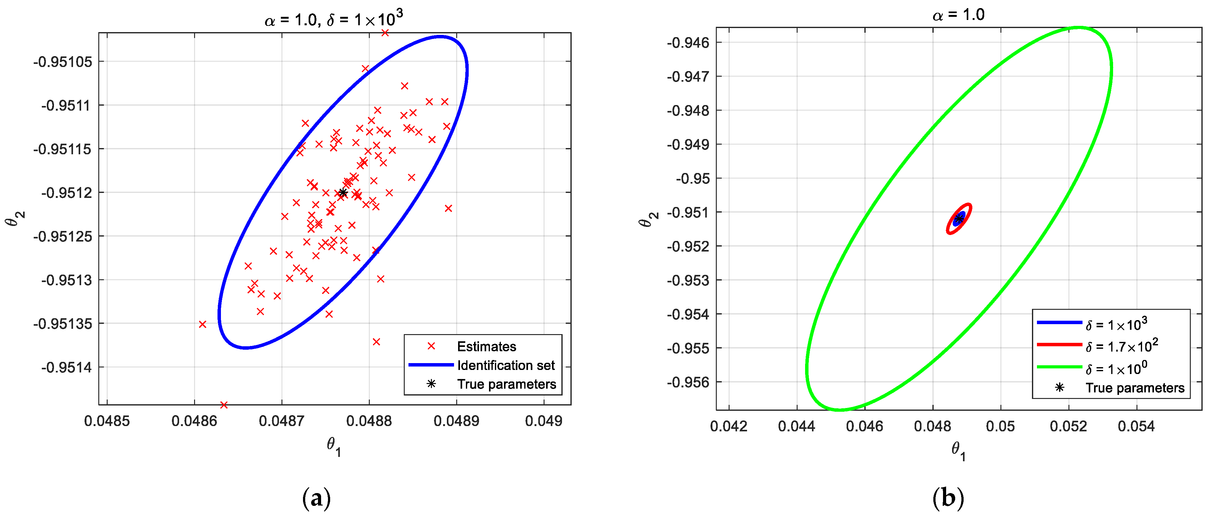
Figure 3 presents the model parameter estimates (32). These have been derived by solving the optimization problem (33) across various values of the input spectrum constraint δ. To identify the parameters of the model (32), we performed 100 independent Monte-Carlo runs.
The system identification set remained within the application set, even with an input spectrum constraint δ = 1 × 100. This has been achieved by assuming a 1% performance degradation with 95% probability. Table 1 shows the mean Absolute Percentage Error (MAPE) for the estimated model parameters, calculated across various input spectrum power constraint values.
Notably, the accuracy of model parameter estimates improves with increased input signal spectrum power when considering the integral-order inertial system. In subsequent experiments, the impact of input signal power on the accuracy of parameter estimates for the fractional-order system is verified.

5.2. Fractional-Order System Identification for α = 0.9

In this section, we focus on fractional-order inertial system identification (29) with α = 0.9 as a key parameter. Using the ORA method for arbitrarily selected bandwidth ω = [10−1, 102] and the order n = 1, we achieved an approximation of the fractional-order operator (9). This result has been converted into a discrete-time output-error (OE) representation (30) with
G 0 q , θ 0 = 0.0156 + 0.0379 q 1 1 0.9397 q 1 ,
We identified the true system’s model using 500 input-output data points, sampled every 0.05 s (Ts = 0.05 s), in the presence of zero-mean white Gaussian noise with variance λ0 = 0.1. The choice of parameters to be estimated is as follows
G q , θ = θ 1 + θ 2 q 1 1 0.9397 q 1 ,       θ = θ 1 , θ 2 T .
Following the conditions outlined in Section 5.1, the application-oriented input design has been performed using formula (33). Figure 4 shows the A-optimal input signal and its spectrum, which have been found for estimating the parameters of model (35) with a power constraint δ = 1 × 10³.
Figure 5 presents the ellipsoidal identification sets obtained using the model (35) by assuming a 1% performance degradation with 95% probability. These have been derived by solving the optimization problem (33) across various values of the input spectrum constraint δ. To estimate the parameters of model (35), we performed 100 independent Monte-Carlo attempts.
The application parameter set no longer meets the criteria of inequality (21) when the input spectrum constraint is δ = 1 × 100. To achieve acceptable accuracy in model parameter estimates, the input spectrum power constraint should be increased. Table 2 presents the calculated MAPEs for the fractional-order model parameters (35), showing how they vary with different input spectrum power constraint values.
To obtain a similar accuracy of the parameter estimates compared to the inertial system (i.e., for α = 1.0), the value of the input signal spectrum power constraint should be increased to the value of δ = 1 × 10³.

5.3. Fractional-Order System Identification for α = 1.1

This section describes a fractional-order inertial system (29) with α = 1.1, representing the order of the system. We estimate the fractional-order operator (9) using the ORA method, under the same assumptions as in the previous section. The discrete-time output-error (OE) model of the system (29) is as follows
G 0 q , θ 0 = 0.0327 0.0262 q 1 1 1.86 q 1 + 0.8663 q 2 ,
To accurately model the system, we applied the identical assumptions as established in the previous part. The parameters to be estimated are
G q , θ = θ 1 + θ 2 q 1 1 1.86 q 1 + 0.8663 q 2 ,       θ = θ 1 , θ 2 T .
We designed the application-oriented input using Formula (33), following the conditions outlined in Section 5.1. Figure 6 displays the A-optimal input signal and its spectrum, which has been obtained for estimating the parameters of the model (37) under a power constraint of δ = 1.7 × 10².
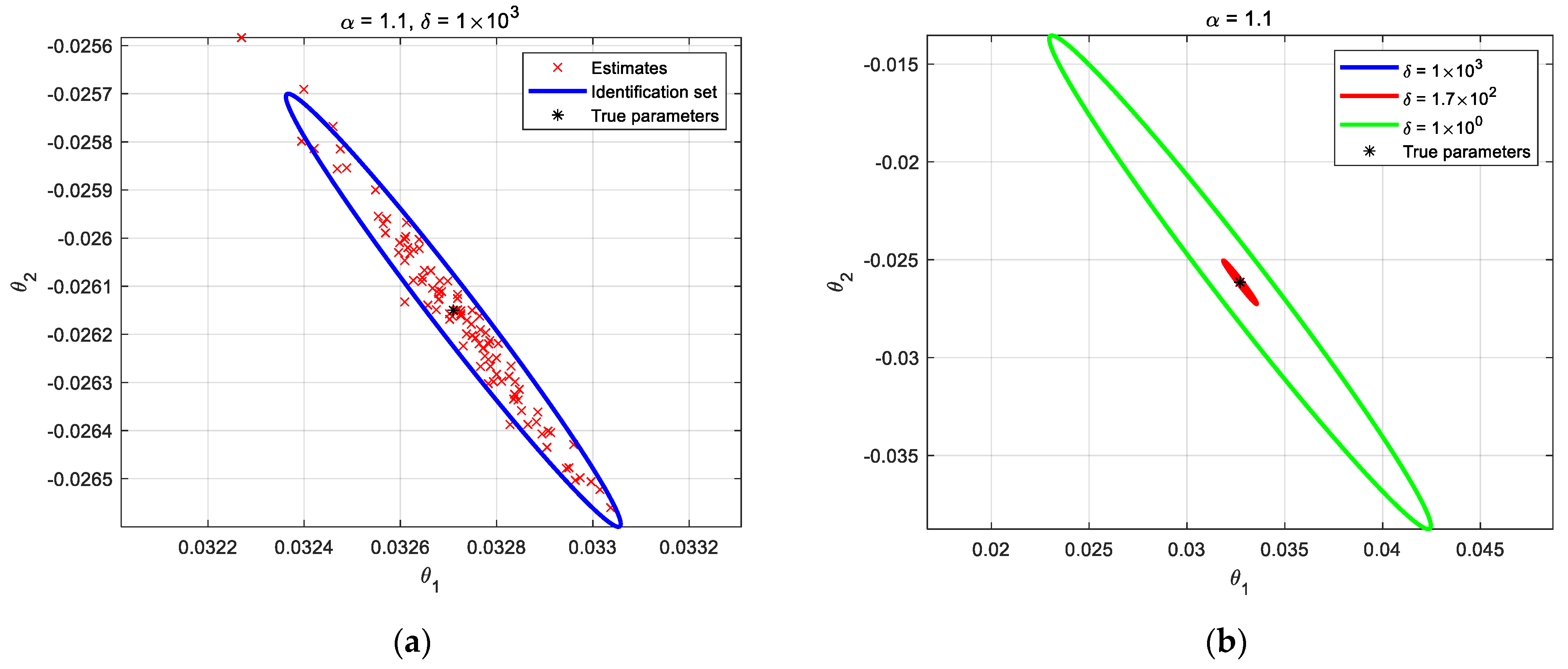
The ellipsoidal identification sets in Figure 7 have been obtained using model (37), under the assumption of a 1% performance degradation with 95% confidence. The derivation involved solving the optimization problem (33) across a range of input spectrum constraints δ. To estimate the parameters of the model (37), we conducted 100 independent Monte-Carlo simulations.
Consistent with the previous situation, the application parameter set violates inequality (21) when the input spectrum constraint is δ = 1 × 100. To obtain sufficiently accurate model parameter estimates, the input spectrum power constraint must be increased. The impact of different input spectrum power constraint values on the MAPEs of the fractional-order model parameters (37) is presented in Table 3.
Increasing the input signal spectrum power constraint to δ = 1.7 × 10² ensures the system identification set remains within the application set. Under these conditions, the parameter estimates show similar accuracy to those of the inertial system (i.e., for α = 1.0).

6. Discussion

The numerical experiments described above aim to determine an approximate input signal power necessary to keep parameter estimates for both integer and fractional-order models within the admissible set of system degradation (21).
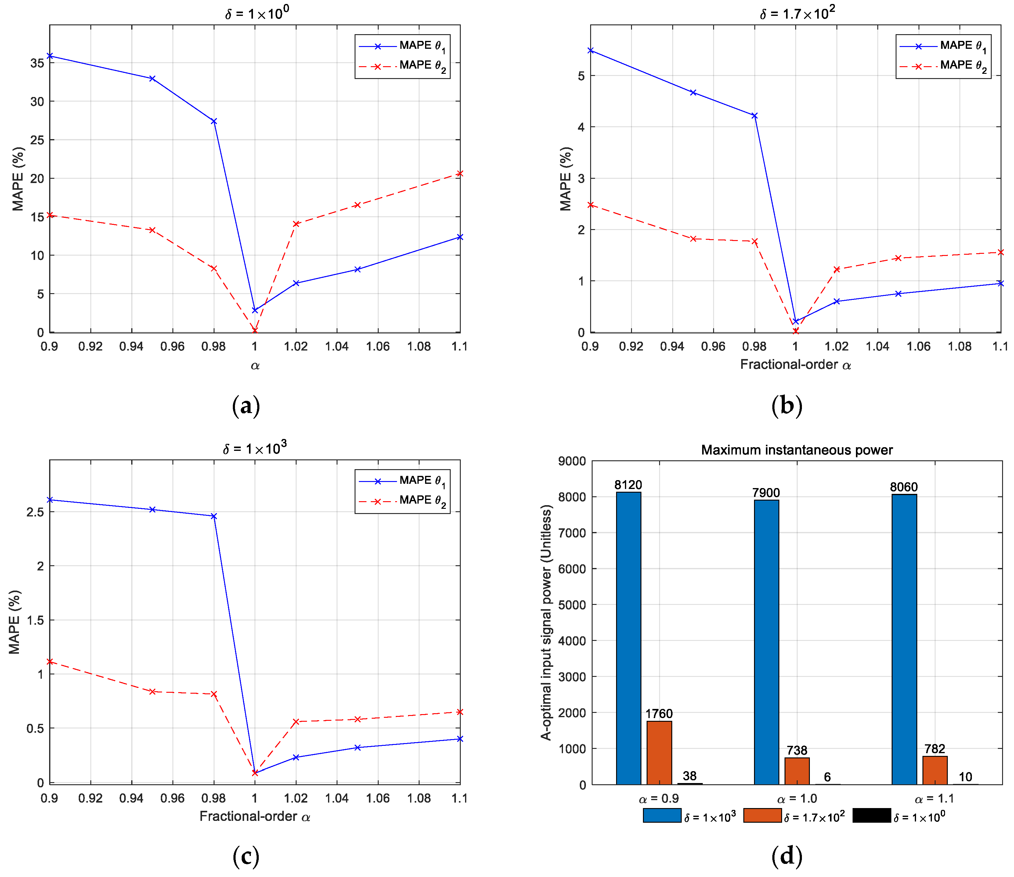
The integer-order inertial system’s identification set remained within the application set, even with a 1.0 × 100 input spectrum constraint (Figure 3). To ensure the identification set remains within the application set for fractional-order systems (i.e., for α = 0.9 and α = 1.1), the input signal spectrum power constraint should be significantly increased. The system identification sets for δ = 1.7 × 10², where these conditions are satisfied, are illustrated in Figure 5 and Figure 7. It can be observed that higher input signal energy leads to more precise parameter estimates in both integer and fractional-order case studies. Figure 8a–c illustrate how the input signal’s spectrum power affects the accuracy of inertial system parameter estimates across various model orders. The integer-order inertial system has yielded the most accurate parameter estimates, as indicated by the smallest MAPEs. As shown in Figure 8d, the maximum instantaneous power of the input signals varied when estimating inertial system parameters for different model orders. The highest instantaneous input signal power has been required to identify the parameters of the fractional-order inertial system, where α = 0.9. The inaccuracy of parameter estimates for the fractional-order models stems from errors introduced during both the ORA and the discretization of continuous-operators.
While fractional-order models have the potential to describe many real-world processes more accurately, their practical implementation through approximations like the ORA method introduces compromises. For the inertial system studied, using approximated fractional-order models often leads to poorer parameter estimates than simpler integer-order models. This is due to inherent issues such as the error from the ORA, limited frequency range, and increased numerical complexity. Despite increasing the frequency range and order of the ORA, the accuracy of the estimated parameters has not improved significantly. The inaccuracy of approximated discrete fractional-order system models stems from the fundamental difference between the infinite-dimensional nature of continuous fractional-order systems and the finite-dimensional representation of discrete systems, along with errors introduced during the discretization process. Fractional-order systems demonstrate memory effects and are highly sensitive to slight changes in input signals or noise. Therefore, achieving accurate parameter estimates typically requires an informative input signal with sufficient energy across the entire frequency spectrum. Poorly designed or noisy input signals are likely to cause significant estimation errors.

7. Conclusions

In this paper, an innovative methodology for designing the optimal input spectrum in open-loop fractional-order system identification is presented. This framework prioritizes the minimization of average input signal power, achieved by combining the established LMI structure with a direct, application-oriented performance measure. The resulting dual optimization problem aims to minimize the input signal power while adhering to constraints that ensure a predefined level of model accuracy. This method uses the recursive ORA method to estimate a fractional-order operator and then estimate the parameters of the resulting integer-order model. To ensure high accuracy of parameter estimates of fractional-order inertial system models, the power constraint of the input signal spectrum should be significantly increased. The validation of the proposed method for identifying approximated fractional-order systems allows us to conclude that a minimal fractional deviation from the integer-order entails a significant increase in the experiment cost in order to maintain its precision.
The method described is limited to open-loop LTI systems. When combined with the ORA, this approach excludes nonlinearities. To address these limitations and ensure comprehensive research, future work should focus on adapting the proposed LMI optimization frameworks for closed-loop identification and developing model order reduction techniques for multidimensional systems. Another promising area for development involves exploring passive identification methods that utilize stochastic phenomena, such as resonance, which could effectively complement the active input design approach discussed.

Author Contributions

Conceptualization, W.J.; methodology, W.J.; software, W.J.; validation, W.J. and M.Ś.; formal analysis, W.J. and M.Ś.; investigation, W.J.; visualization, W.J.; writing—original draft preparation, W.J. and M.Ś. All authors have read and agreed to the published version of the manuscript.

Funding

The present study was supported by grants WZ/WI-IIT/5/2023 (W. Jakowluk) and WZ/WE-IA/5/2023 (M. Świercz) from Bialystok University of Technology and was funded from the research resources provided by the Ministry of Science and Higher Education.

Data Availability Statement

The authors confirm that all data generated or analyzed during this study are included within the entirety of this presented article.

Conflicts of Interest

The authors declare no conflicts of interest.

References

  1. Kalaba, R.; Spingarn, K. Control, Identification, and Input Optimization, 1st ed.; Springer: New York, NY, USA, 2012. [Google Scholar]
  2. Sánchez-Peña, R.S.; Quevedo Casín, J.; Puig Cayuela, V. Identification and Control. The Gap Between Theory and Practice; Springer-Verlag: London, UK, 2007. [Google Scholar]
  3. Ikonen, E.; Najim, K. Advanced Process Identification and Control; Taylor and Francis: Boca Raton, FL, USA, 2019. [Google Scholar]
  4. Gevers, M. Identification for Control: From the Early Achievements to the Revival of Experiment Design. Eur. J. Control 2005, 11, 335–352. [Google Scholar] [CrossRef]
  5. Bombois, X.; Scorletti, G.; Gevers, M.; Van den Hof, P.M.J.; Hildebrand, R. Least costly identification experiment for control. Automatica 2006, 42, 1651–1662. [Google Scholar] [CrossRef]
  6. Annergren, M.; Larsson, C.A.A.; Hjalmarsson, H.; Bombois, X.; Wahlberg, B. Application-oriented input design in system identification: Optimal input design for control. IEEE Control Syst. Mag. 2017, 37, 31–56. [Google Scholar] [CrossRef]
  7. Kumar, A.; Narasimhan, S. Robust plant friendly optimal input design. In Proceedings of the 2013 International Symposium on Dynamics and Control of Process Systems (IFAC), Mumbai, India, 18–20 December 2013. [Google Scholar]
  8. Narasimhan, S.; Rengaswamy, R. Plant friendly input design: Convex relaxation and quality. IEEE Trans. Automat. Contr. 2011, 56, 1467–1472. [Google Scholar] [CrossRef]
  9. Rivera, D.E.; Lee, H.; Braun, M.W. ‘Plant-friendly’ system identification: A challenge for the process industries. In Proceedings of the 2003 Symposium on System Identification (IFAC), Rotterdam, The Netherlands, 27–29 September 2003. [Google Scholar]
  10. Rafajłowicz, E. Optimal Input Signals for Parameter Estimation: In Linear Systems with Spatio-Temporal Dynamics; De Gruyter: Berlin, Germany; Boston, MA, USA, 2022. [Google Scholar]
  11. Oustaloup, A.; Levron, F.; Mathieu, B.; Nanot, F. Frequency-band complex noninteger differentiator: Characterization and synthesis. IEEE Trans. Circuits Syst. I Fundam. Theory Appl. 2000, 47, 25–39. [Google Scholar] [CrossRef]
  12. Stanisławski, R.; Rydel, M.; Latawiec, K.J. Modeling of discrete-time fractional order state space systems using the balanced truncation method. J. Frankl. Inst. Eng. Appl. Math. 2017, 354, 3008–3020. [Google Scholar] [CrossRef]
  13. Jakowluk, W. Optimal Input Signal Design in Control Systems Identification; Publishing House of Bialystok University of Technology: Bialystok, Poland, 2024. [Google Scholar]
  14. Malti, R.; Mayoufi, A.; Victor, S. Experiment design for elementary fractional models. Commun. Nonlinear Sci. Numer. Simul. 2022, 110, 106337. [Google Scholar] [CrossRef]
  15. Ljung, L. System Identification: Theory for the User; Prentice Hall, Inc.: Upper Saddle River, NJ, USA, 1999. [Google Scholar]
  16. Victor, S.; Mayoufi, A.; Malti, R.; Chetoui, M.; Aoun, M. System identification of MISO fractional systems: Parameter and differentiation order estimation. Automatica 2022, 141, 110268. [Google Scholar] [CrossRef]
  17. Victor, S.; Duhe, J.; Melchior, P.; Abdelmoumen, Y.; Roubertie, F. Long memory recursive prediction error method for identification of continuous-time fractional models. Nonlinear Dynam. 2022, 110, 635–648. [Google Scholar] [CrossRef]
  18. Ning, B.; Han, Q.L. Prescribed Finite-Time Consensus Tracking for Multiagent Systems With Nonholonomic Chained-Form Dynamics. IEEE Trans. Autom. Control 2019, 64, 1686–1693. [Google Scholar] [CrossRef]
  19. Abrashov, S.; Malti, R.; Moze, M.; Moreau, X.; Guillemard, F. Optimal input design for continuous-time system identification: Application to fractional systems. In Proceedings of the 2015 Symposium on System Identification SYSID (IFAC), Beijing, China, 19–21 October 2015. [Google Scholar]
  20. Abrashov, S.; Malti, R.; Moreau, X.; Moze, M.; Aioun, F.; Guillemard, F. Optimal input design for continuous-time system identification. Commun. Nonlinear Sci. Numer. Simul. 2018, 60, 92–99. [Google Scholar] [CrossRef]
  21. Stanisławski, R. Fractional dynamical systems: Methods, algorithms and applications. In Studies in Systems, Decision and Control; Kulczycki, P., Korbicz, J., Kacprzyk, J., Eds.; Springer: Cham, Germany, 2022; Volume 402, pp. 3–25. [Google Scholar]
  22. Monje, C.A.; Chen, Y.; Vinagre, B.; Xue, D.; Feliu, V. Fractional Orders Systems and Controls: Fundamentals and Applications; Springer-Verlag: London, UK, 2010. [Google Scholar]
  23. Ljung, L. System Identification Toolbox: User’s Guide; The MathWorks, Inc.: Natick, MA, USA, 2010. [Google Scholar]
  24. Hjalmarsson, H. System identification of complex and structured systems. Eur. J. Control 2009, 15, 275–310. [Google Scholar] [CrossRef]
  25. Jansson, H.; Hjalmarsson, H. Input design via LMIs admitting frequency wise model specifications in confidence regions. IEEE Trans. Autom. Control 2005, 50, 1534–1549. [Google Scholar] [CrossRef]
  26. Boyd, S.; Vandenberghe, L. Convex Optimization; Cambridge Univ. Press: Cambridge, UK, 2004. [Google Scholar]
  27. Li, S.; Deng, Q.; Li, Z.; Hu, W. Control-oriented closed-loop identification and input design in a wireless power transfer system. WPT 2025, 12, e007. [Google Scholar] [CrossRef]
  28. Jakowluk, W.; Świercz, M. Application-oriented input spectrum design in closed-loop identification. Appl. Sci. 2023, 13, 6552. [Google Scholar] [CrossRef]
  29. Jakowluk, W.; Jaszczak, S. Cascade tanks system identification for robust predictive control. Bull. Pol. Acad. Sci. Technol. Sci. 2022, 70, e143646. [Google Scholar] [CrossRef]
  30. Annergren, M.; Larsson, C.A. MOOSE2: Model Based Optimal Input Signal Design Toolbox. Version 2, Sweden, 2015. Available online: https://www.kth.se/is/dcs/research/sysid/moose/moose2-toolbox-1.194509 (accessed on 9 November 2025).
  31. Löfberg, J. YALMIP: A toolbox for modeling and optimization in MATLAB. In Proceedings of the Computer Aided Control System Design Conference, Taipei, Taiwan, 2–4 September 2002. [Google Scholar]
  32. Toh, K.C.; Todd, M.J.; Tütüncü, R.H. On the Implementation and Usage of SDPT3—A Matlab Software Package for Semidefinite-Quadratic-Linear Programming, Version 4.0. In Handbook of Semidefinite, Conic and Polynomial Optimization; Anjos, M.F., Lasserre, J.B., Eds.; Springer: Boston, MA, USA, 2012; pp. 715–754. [Google Scholar]
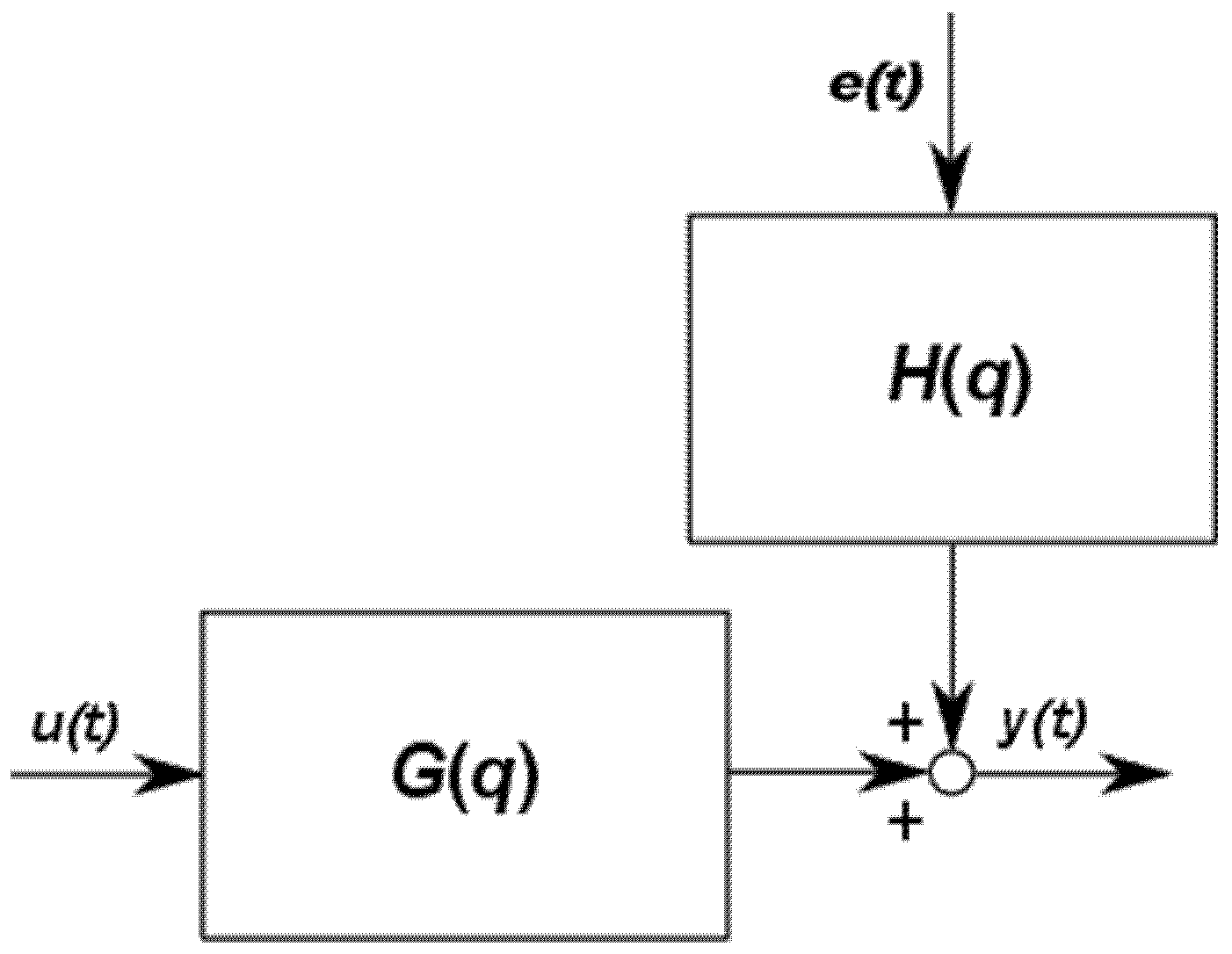
Figure 1. The open-loop system diagram.
Applsci 15 12665 g001
Figure 2. Application-oriented input design for δ = 1 × 100: (a) Refers to the A-optimal input signal energy within a given time interval; (b) Bode plot of the A-optimal input spectrum magnitude and phase.
Applsci 15 12665 g002
Figure 3. (a) The system identification set for constrained A-optimal input design δ = 1 × 10³; (b) The ellipsoidal regions obtained for different A-optimal input design constraints δ.
Applsci 15 12665 g003
Figure 4. Application-oriented input design for δ = 1 × 10³: (a) Refers to the A-optimal input signal energy within a given time interval; (b) Bode plot of the A-optimal input spectrum magnitude and phase.
Applsci 15 12665 g004
Figure 5. (a) The system identification set for constrained A-optimal input design δ = 1 × 10³; (b) The ellipsoidal regions obtained for different A-optimal input design constraints δ.
Applsci 15 12665 g005
Figure 6. Application-oriented input design for δ = 1.7 × 10²: (a) Refers to the A-optimal input signal energy within a given time interval; (b) Bode plot of the A-optimal input spectrum magnitude and phase.
Applsci 15 12665 g006
Figure 7. (a) The system identification set for constrained A-optimal input design δ = 1 × 10³; (b) The ellipsoidal regions obtained for different A-optimal input design constraints δ.
Applsci 15 12665 g007
Figure 8. The impact of input signal power on parameter estimation precision: (ac) MAPE of parameter estimates across varying system orders α; (d) Maximum instantaneous power for various input signal constraints δ.
Applsci 15 12665 g008
Table 1. MAPE for estimated inertial model parameters (i.e., α = 1.0).
δ/θ1 × 1001.7 × 1021 × 103
θ12.842%0.213%0.086%
θ20.225%0.017%0.006%
Table 2. MAPE for estimated inertial model parameters (i.e., α = 0.9).
δ/θ1 × 1001.7 × 1021 × 103
θ135.875%5.485%2.270%
θ216.138%2.479%0.888%
Table 3. MAPE for estimated inertial model parameters (i.e., α = 1.1).
δ/θ1 × 1001.7 × 1021 × 103
θ112.366%0.951%0.401%
θ220.617%1.557%0.653%
Disclaimer/Publisher’s Note: The statements, opinions and data contained in all publications are solely those of the individual author(s) and contributor(s) and not of MDPI and/or the editor(s). MDPI and/or the editor(s) disclaim responsibility for any injury to people or property resulting from any ideas, methods, instructions or products referred to in the content.