Article

Bayesian Network-Driven Demand Prediction and Multi-Trip Two-Echelon Routing for Fleet-Constrained Metropolitan Logistics

School of Economics & Management, Tongji University, Shanghai 200092, China
*
Author to whom correspondence should be addressed.
Appl. Sci. 2025, 15(23), 12609; https://doi.org/10.3390/app152312609
Submission received: 20 October 2025 / Revised: 17 November 2025 / Accepted: 25 November 2025 / Published: 28 November 2025
(This article belongs to the Special Issue Explainable Artificial Intelligence Technology and Its Applications)

Abstract

Urban logistics in metropolitan areas faces mounting pressure to deliver faster while controlling operational costs under strict fleet size constraints. Traditional vehicle routing models assume unlimited vehicle availability, overlooking realistic fleet utilization and spatial-temporal demand imbalances. This paper introduces the fleet-constrained metropolitan logistics problem (FCMLP), a novel framework integrating trunk linehaul scheduling, two-echelon routing, multi-trip operations, and anticipatory fleet positioning. We model the FCMLP as a Markov Decision Process capturing the stochastic and dynamic nature of metropolitan delivery flows. Our solution framework combines interpretable Bayesian Network-based demand forecasting for transparent proactive vehicle relocation decisions, parameterized cost-function approximation for dynamic order-to-linehaul assignment, and Adaptive Large Neighborhood Search for multi-trip vehicle routing. Computational experiments on synthetic instances and real-world data from a major e-commerce platform in Jakarta demonstrate 20–26% total cost reduction. Multi-trip operations alone reduce fleet size by 23%, while interpretable predictive relocation further improves performance by 7% through a 20% reduction in emergency deployments. The framework’s interpretability enhances operator trust and facilitates practical adoption, offering logistics platforms a path to improve vehicle utilization through operational efficiency and transparent predictive intelligence without expanding fleet size.

1. Introduction

The rapid growth of e-commerce has transformed urban logistics operations in metropolitan areas worldwide. With global parcel volumes growing over 50% annually, logistics providers face mounting pressure to deliver faster while managing operational costs. This challenge is particularly acute in densely populated metropolitan regions, where multiple cities interconnect through complex transportation networks. While major e-commerce platforms have established sophisticated logistics networks, they face increasing pressure to optimize fleet utilization as vehicle acquisition and maintenance represent substantial capital investments. The dynamic nature of e-commerce demand, with characteristic spatial-temporal imbalances across urban districts, further complicates efficient resource allocation and necessitates intelligent fleet management strategies.
Efficient fleet utilization has emerged as a critical operational priority. While existing literature often assumes unlimited vehicle availability, practical operations require careful management of fleet resources. For large operators, optimizing fleet size yields significant cost savings and environmental benefits. For small and medium-sized providers, working within fixed fleet constraints is necessity-driven by capital limitations. This convergence creates a universal need for strategies maximizing existing vehicle asset productivity. The challenge extends beyond static optimization to encompass dynamic adaptation, where predictive capabilities and proactive resource positioning become essential for maintaining service quality while ensuring transparent reasoning that operators can understand and trust.
Two-echelon distribution structures, commonly adopted in metropolitan areas, feature parcels flowing from suppliers to city hubs, then to satellite facilities, before final customer delivery. This hub-satellite-customer structure enables consolidation for efficient middle-mile transport and deploys smaller vehicles for congested urban streets. The two-echelon vehicle routing problem (2E-VRP) has been comprehensively reviewed by Sluijk et al. [1]. By placing reload points near customer clusters, satellites dramatically reduce reload time, synergistically enabling multi-trip routing where vehicles complete multiple pickup and delivery cycles within operational periods.
Multi-trip mechanisms offer powerful solutions for improving fleet efficiency. By relaxing traditional “one vehicle, one route per day” assumptions, the Multi-Trip Vehicle Routing Problem (VRPMT) enables operators to serve more customers with existing fleets, as surveyed by Cattaruzza et al. [2]. Recent research has integrated multi-trip operations into two-echelon models [3,4]. However, implementing multi-trip operations within metropolitan logistics presents complex coordination challenges requiring sophisticated planning that considers vehicle capacity, time windows, and dynamic fleet repositioning, with effectiveness relying on providing clear operational decision explanations.
This paper addresses these challenges by proposing an integrated optimization framework for metropolitan logistics that maximizes vehicle utilization through multi-trip strategies and predictive fleet management. We formalize this as the fleet-constrained metropolitan logistics problem (FCMLP), modeling it as a Markov Decision Process (MDP) that captures stochastic order arrivals and sequential decision-making. Our approach integrates interpretable Bayesian Network-based demand prediction for proactive relocation, parameterized Cost Function Approximation (CFA) for dynamic order assignment, and Adaptive Large Neighborhood Search (ALNS) for multi-trip routing. To the best of our knowledge, this is the first work integrating (i) explicit fleet constraints in two-echelon multi-trip frameworks; (ii) interpretable Bayesian Network-based prediction for proactive relocation; (iii) dynamic order-to-linehaul assignment with multi-trip delivery under stochastic demand; and (iv) unified MDP formulation capturing component interactions.
The main contributions are (1) formulating the FCMLP with explicit fleet constraints and multi-trip operations while incorporating interpretable predictive analytics; (2) developing an adaptive MDP-based framework coordinating Bayesian Networks for demand prediction, parameterized cost functions for order assignment, enhanced ALNS for multi-trip routing, and hierarchical Bayesian optimization; and (3) demonstrating through experiments on synthetic instances and real-world Jakarta e-commerce data that multi-trip operations achieve 22.6% fleet reduction and 20.5% cost reduction, with proactive relocation providing additional benefits.
The paper is organized as follows: Section 2 reviews relevant literature. Section 3 defines the problem and mathematical formulation. Section 4 details our solution methodology. Section 5 presents computational experiments. Section 6 discusses findings and future research.

2. Literature Review

Modern metropolitan logistics complexity demands sophisticated optimization frameworks. This review analyzes three critical streams: (1) multi-trip vehicle routing under fleet constraints; (2) two-echelon vehicle routing with multi-trip capabilities; and (3) dynamic stochastic dispatching. We systematically examine these domains to identify significant gaps at their intersection.

2.1. Multi-Trip Vehicle Routing Under Fleet Constraints

The VRPMT relaxes single-tour constraints, allowing vehicles to perform subsequent trips after reloading. Cattaruzza et al. [2] provide foundational VRPMT formulation overviews. Recent research increasingly recognizes explicit fleet constraints as operators optimize fleet size. Hernandez et al. [5] demonstrated significant fleet reductions through multi-trip strategies. Zhen et al. [6] extended this to multi-depot settings with release dates, combining features "seldom considered simultaneously."
Strategic fleet planning integration has emerged as crucial. Fermín Cueto et al. [7] divide problems into strategic (depot allocation, fleet sizing) and operational planning for robustness. Chen et al. [8] address heterogeneous fleets under budget constraints, showing 17.54% cost reduction. Karademir et al. [9] demonstrate multi-trip benefits in integrated water-land transportation. Pan et al. [10] incorporate time-dependent speeds through adaptive large neighborhood search.
However, these studies remain limited to single-echelon networks or static planning, unable to capture unique fleet utilization opportunities that two-echelon structures provide through satellites near customer clusters.

2.2. Two-Echelon Routing with Satellite Reload Points

Two-echelon systems enable first-echelon consolidation and second-echelon agility. Sluijk et al. [1] comprehensively review 2E-VRP literature. Satellites near customer clusters reduce reload time versus single-echelon systems, making multiple trips economically attractive. Grangier et al. [11] pioneered two-echelon multi-trip VRP with satellite synchronization.
Satellite concepts evolved beyond traditional transshipment. Enthoven et al. [12] introduce parcel lockers as covering locations. Li et al. [13] address bi-synchronization at origin and destination satellites. Dos Santos et al. [14] use lockers with occasional couriers for last-mile flexibility. Dahimi et al. [15] innovate with mobile satellites serving dual vehicle-transshipment roles.
Multi-trip integration advances include Dumez et al. [3] allowing first-echelon multi-trips with reverse flows, and Lehmann & Winkenbach [4] focusing on second-echelon multi-trips. Tadaros & Kyriakakis [16] handle hierarchical multi-switch systems. Gutierrez et al. [17] incorporate time-dependent travel times. Zamal et al. [18] merge first and last-mile operations. Şahin & Yaman [19] explicitly address limited fleet size in two-echelon systems. Guo et al. [20] study front warehouse models with transshipment constraints.
Despite structural sophistication, these models assume static demand and rarely treat fleet constraints as primary objectives.

2.3. Dynamic and Stochastic Dispatch Under Fleet Limitations

Dynamic modeling addresses uncertainty through Markov Decision Processes. Crainic et al. [21] address capacity planning through stochastic bin packing. Ghilas et al. [22] combine stochastic demands with scheduled lines.
Real-time dispatching requires sophisticated strategies. Klapp et al. [23] formulate Dynamic Dispatch Waves Problems where reactive optimization reduces costs while improving coverage. Van Heeswijk et al. [24] use approximate dynamic programming for urban consolidation centers.
Advanced methodologies handle continuous-time operations. He et al. [25] adapt Dynamic Discretization Discovery for retail distribution. Medina et al. [26] integrate long-haul and local planning. Zamal et al. [27] present Stochastic Dynamic Order-Assignment using MDPs with cost function approximation. Sluijk et al. [28] formulate chance-constrained 2E-VRP. Recent spatiotemporal prediction advances show promise: Cai et al. [29] develop JointSTNet for traffic forecasting; Beni Prathiba et al. [30] propose Digital Twin-enabled optimization achieving 30% congestion reduction.
However, these frameworks focus on information flow without explicitly modeling fixed fleet constraints. When fleet is limited, objectives shift from cost minimization to maximizing scarce resource throughput.

2.4. Bayesian Networks for Supply Chain Risk and Demand Prediction

Bayesian networks provide transparent probabilistic frameworks for uncertainty in supply chains. Garvey et al. [31] model networked risk dependencies. Extensions include: Hosseini et al. [32] integrate DTMC with DBNs for supplier ripple effects; Liu et al. [33] address data scarcity via robust DBNs; Liu et al. [34] employ signomial programming for multi-echelon assessment. For extreme scenarios, Hosseini & Ivanov [35] develop multi-layer BNs for pandemics; Liu et al. [36] propose structure-variable DBNs for viability adaptation. Operations applications include: Attar et al. [37] enable what-if analysis; Harikrishnakumar & Nannapaneni [38] explore quantum BNs for demand prediction; Liu et al. [39] introduce risk-averse DBNs; Liang et al. [40] employ BNs for adaptive eco-cruising control.
Existing BN work emphasizes strategic assessment or stand-alone prediction; few studies operationalize interpretable BN posteriors for real-time resource allocation under fleet constraints.

2.5. Research Gap

Analysis reveals significant gaps at the confluence of multi-trip routing, two-echelon structures, and dynamic-stochastic operations. While individual elements have been studied, no framework provides integrated solutions capturing interdependencies. Furthermore, BN interpretability advantages are seldom operationalized for proactive fleet management. Our research bridges this gap by introducing FCMLP as a unified framework integrating explicit fleet constraints, multi-trip operations within two-echelon networks, dynamic stochastic order arrivals, interpretable BN-based prediction for proactive allocation, and transparent decision-making building operator trust. Table 1 summarizes differences between prior work and this study.

3. Model

This section presents the mathematical formulation of the FCMLP introduced above. We begin with a detailed description of the system components and operational characteristics, followed by the formulation as a Markov Decision Process (MDP) following the framework introduced by Powell [41]. A complete list of notation is provided in Supplementary Materials S1.

3.1. Problem Description

The FCMLP considers logistics operations across multiple cities z Z within a metropolitan area, where predictive analytics and proactive resource management are essential for maintaining service quality under fleet constraints. The core challenge extends beyond traditional reactive routing to encompass anticipatory decision-making: leveraging interpretable machine learning models to predict spatial-temporal demand patterns and proactively repositioning idle vehicles before demand materializes.
Each stochastic and dynamic order o O is characterized by demand size q o , pickup location p o at ( X p o , Y p o ) in origin city z o fm , and delivery location d o at ( X d o , Y d o ) in destination city z o lm . Both locations have hard time windows [ E p o , L p o ] and [ E d o , L d o ] , respectively.
The logistics system employs two-echelon vehicle routing within each city. First-echelon vehicles with capacity Q z 1 operate between hubs and satellites, while second-echelon vehicles with capacity Q z 2 handle final distribution from satellites to customers. Each city z maintains a limited fleet of | V z 2 | homogeneous second-echelon vehicles distributed across satellites. This fleet size is a strategic decision variable balancing operational costs against service requirements. Routing decisions are made independently within each city.
Vehicle operations require service time φ at each customer/supplier location and reload time ρ at satellites for multi-trip operations, after which vehicles are immediately available for subsequent trips. Second-echelon vehicles start each trip from their current satellite location, which can change over time through proactive relocation. Pre-scheduled linehaul services L connect city hubs with departure time t ¯ , capacity Q , fixed cost F , and variable cost U per unit weight.
The dynamic nature of metropolitan demand creates significant spatial–temporal imbalances across satellites. To address this, we incorporate side information I k , including historical patterns, temporal features, and area characteristics. This feeds into an interpretable Bayesian Network predicting future demand distribution, enabling proactive vehicle relocation that positions resources where they will be needed rather than where they were last used.
To maximize limited fleet productivity, vehicles perform multiple trips within the planning horizon T = [ 0 , T ] . Strategic satellite placement near customer clusters reduces reload-related travel compared to central depot returns, making multi-trip operations economically viable.
Operating costs include daily fixed cost c z fixed per regular vehicle and variable cost c z var per distance unit. When the regular fleet cannot meet time windows, emergency vehicles are deployed at significantly higher costs ( c em , fixed and c em , var ), creating the fundamental trade-off between fleet size and emergency deployment frequency.
The objective is to determine (1) the optimal second-echelon fleet size | V z 2 | for each city and (2) a real-time operational policy coordinating order-to-linehaul assignments and multi-trip routing to minimize the total expected cost over the planning horizon.
Key Assumptions:
1.
Unlimited First-Echelon Fleet Size: The number of first-echelon vehicles operating between hubs and satellites is assumed to be unlimited. This reflects the fundamental difference in operational characteristics between the two echelons: first-echelon vehicles operate on predictable routes between fixed facilities (hubs and satellites) with consolidated loads, enabling efficient capacity planning and flexible fleet adjustment through third-party logistics providers or on-demand vehicle leasing. This assumption transforms the dynamic first-echelon routing into a sequence of independent static optimization problems, where each epoch’s routing decisions are made without tracking vehicle states or availability constraints. In contrast, second-echelon vehicles must navigate dynamic customer-specific routes with strict time windows, requiring dedicated local resources and specialized knowledge of the service area.
2.
Fixed Second-Echelon Fleet During Operations: The second-echelon fleet size remains constant throughout the operational period. Vehicle acquisition and disposal decisions cannot be made in real-time due to capital investment lead times and labor contracts.
3.
Deterministic Travel Times: Travel times between locations are known and constant. While this simplification is common in strategic fleet sizing problems and aligns with standard VRP literature, we partially capture real-world traffic variations through time-dependent linehaul capacity adjustments during peak (80% capacity) and off-peak (120% capacity) periods. This approach balances model tractability with operational realism for the core fleet sizing and multi-trip coordination challenges.
4.
No Split Deliveries: Each order must be handled entirely by a single vehicle. This maintains operational simplicity and package tracking integrity, reflecting standard practice in parcel delivery operations.
5.
Predictable Demand Patterns: Order arrivals exhibit spatial-temporal patterns that can be learned from historical data and side information. While individual orders remain stochastic, aggregate demand at the satellite level shows sufficient regularity to enable meaningful predictions through our Bayesian Network approach.
6.
Relocation Time Windows: Vehicle relocations can only occur during idle periods and must be complete before the vehicle’s next anticipated assignment. This ensures that proactive positioning does not interfere with active service commitments.
These assumptions balance model realism with analytical tractability, focusing on the critical challenge of maximizing limited second-echelon fleet utilization through integrated multi-trip strategies and predictive fleet management in two-echelon metropolitan logistics networks.

3.2. Markov Decision Process

This section formulates the problem as a hierarchical optimization problem. In the first stage, we determine the second-echelon fleet sizes for each city. In the second stage, we model the operational decisions as an MDP given the fixed fleet sizes.
Stage 1—Strategic Fleet Sizing: Before the operational period begins, determine the second-echelon fleet size | V z 2 | for each city z Z . This decision incurs a fixed daily operating cost C fleet ( | V z 2 | ) that includes driver wages, insurance, and maintenance. Specifically,
C fleet ( | V z 2 | ) = z Z c z fixed · | V z 2 |
Stage 2—Operational Decisions: Given the fleet sizes from Stage 1, we model the dynamic operational decisions as an MDP. The system is observed at discrete decision epochs k K : = { 0 , , K } , occurring at equidistant time intervals δ between all epochs.
State Variable: At each decision epoch k, the system state captures both operational status and predictive information to enable proactive fleet management. The state variable S k S is defined as
S k = ( t k , o k fm , o k mm , t k mm , o k lm , t k lm , L z k , v k , I k )
where the components are organized into the following three categories:
Temporal and Order Information:
  • t k T is the current time at decision epoch k.
  • o k fm is a vector of order indices ready for first-mile pickup in each city.
  • o k mm and t k mm are vectors of orders awaiting middle-mile linehaul shipment and their arrival times at origin hubs.
  • o k lm and t k lm are vectors of orders awaiting last-mile delivery and their arrival times at destination hubs.
  • L z k denotes the set of linehauls departing after time t k from city z.
Vehicle Status Information:
  • v k = { ( γ v current , s t a t u s v , t v avail ) } v V z 2 , z Z represents the status of second-echelon vehicles, where the following apply:
    -
    γ v current G z is the current satellite location of vehicle v.
    -
    s t a t u s v { i d l e , r o u t i n g , r e l o c a t i n g } is the operational status.
    -
    t v avail is the time when the vehicle becomes available for new assignments.
Side Information for Predictive Analytics:
  • I k = { I γ k } γ G contains satellite-specific side information, where each I γ k = ( H γ k , A γ , N γ k nd , E γ k ) includes the following:
    -
    H γ k R + : historical average demand at satellite γ for similar time periods over the past few days.
    -
    A γ { Type 1 , Type 2 , Type 3 } : satellite area classification.
    -
    N γ k nd Z + : number of pending next-day orders currently assigned to satellite γ .
    -
    E γ k { 0 , 1 } : binary indicator for special events near satellite γ .
This enhanced state representation enables the system to leverage historical patterns and current operational status for anticipatory decision-making, particularly for proactive vehicle positioning based on predicted demand surges.
Decision Variables: The decision x k X ( S k ) comprises the following three key components for each city z:
1.
Order Assignment: Binary variables a ^ o z k { 0 , 1 } indicating if order o o k fm o k mm is assigned to linehaul L z k .
2.
Vehicle Dispatch and Routing: Selecting subset o k r o k fm o k lm and determining multi-trip routes for available second-echelon vehicles, with binary variables y ^ r z k { 0 , 1 } indicating if route r z k is executed.
3.
Proactive Vehicle Relocation: To address predicted demand imbalances across satellites, the system can proactively relocate idle vehicles. Binary variables r ^ v γ z k { 0 , 1 } indicate whether idle vehicle v is relocated from its current satellite to satellite γ in city z at epoch k. These relocation decisions are subject to the following operational constraints:
  • Each idle vehicle can be relocated to at most one destination: γ G z r ^ v γ z k 1 , v V z idle .
  • Only vehicles with s t a t u s v = i d l e are eligible for relocation.
  • Relocations occur only between satellites within the same city: r ^ v γ z k = 0 if γ G z where v V z 2 .
  • To prevent cascading relocations, vehicles relocated in the previous epoch cannot be relocated again: if γ r ^ v γ , z , k 1 = 1 , then γ r ^ v γ z k = 0 .
Immediate Cost Function: The cost incurred at epoch k given state S k and decision x k comprises four components,
C ( S k , x k ) = c ^ k A C + c ^ k R C + c ^ k E C + c ^ k R L C
where the cost components are defined as follows:
  • c ^ k A C is the linehaul assignment cost,
    c ^ k A C = z Z L z k F w ^ z k + o o k l L z k q o U a ^ o z k
    where o k l = o k fm o k mm represents all orders eligible for linehaul assignment, and w ^ z k { 0 , 1 } indicates whether linehaul is used.
  • c ^ k R C is the regular vehicle routing cost,
    c ^ k R C = z Z r z k R z k 2 c z var · d i s t ( r z k ) · y ^ r z k
    where R z k 2 is the set of second-echelon routes in city z at epoch k, and d i s t ( r z k ) denotes the total distance of route r z k .
  • c ^ k E C is the emergency transportation cost,
    c ^ k E C = o O k violated ( c em , fixed + c em , var · d i s t o e m )
    where O k violated is the set of orders that cannot be served within time windows by the regular fleet, and d i s t o e m is the emergency vehicle travel distance for order o.
  • c ^ k R L C is the proactive relocation cost, representing the operational expense of repositioning vehicles between satellites,
    c ^ k R L C = z Z v V z idle γ G z c z var · d i s t ( γ v current , γ ) · r ^ v γ z k
    where V z idle = { v V z 2 : s t a t u s v = i d l e } represents the set of currently idle vehicles in city z, and d i s t ( γ v current , γ ) is the distance between the vehicle’s current satellite and the target satellite.
The routing decision must satisfy the following constraints for fleet size and multi-trip operations:
r z k R z k 2 y ^ r z k | V z 2 | , z Z
For multi-trip operations, vehicles can perform multiple routes within the planning horizon, subject to time feasibility constraints. A vehicle v can be assigned to a route r only if
s r t v avail , r R v k , v V z 2
where R v k is the set of feasible routes for vehicle v at epoch k, and s r is the start time of route r. The end time of route r, denoted as e r , includes the travel time between all nodes in the route plus the service time φ at each customer or supplier location visited. After completing route r, vehicle v becomes available at time
t v avail = e r + ρ
where ρ is the reload time at the satellite. Furthermore, all routes must be completed within the planning horizon
e r T , r R z k 2
When Equations (8), (9), (10), and (11) cannot accommodate all orders within their time windows, the excess orders in O k violated must be served by emergency vehicles at significantly higher costs. This cost differential—with c em , fixed > > c z fixed and c em , var > c z var —creates the fundamental trade-off: larger regular fleets reduce expensive emergency deployments but increase daily fixed costs, while smaller fleets save on fixed costs but may trigger frequent costly emergency vehicle usage.
Additionally, vehicle operations must respect location constraints
γ v i = γ v current , v V z 2 , new trips T v i
where γ v i is the departure satellite for vehicle v’s i-th trip. This ensures vehicles can only start new trips from their current location.
For vehicle relocation, the following constraints apply:
γ G z r ^ v γ z k 1 , v V z idle , z Z
ensuring each idle vehicle is relocated to at most one satellite per epoch.
The relocation must complete before the vehicle’s next potential assignment,
t k + d i s t ( γ v current , γ ) speed t v next , v : r ^ v γ z k = 1
where t v next is the earliest time the vehicle might be needed based on predicted demand.
Exogenous Information: The exogenous information variable W k + 1 ( S k , x k ) captures the arrival of new orders o k + 1 new in the system at decision epoch k + 1 .
Transition Function: The transition function S k + 1 = S M ( S k , x k , W k + 1 ) describes the system’s evolution, with vehicle status updates now incorporating relocation decisions,
v k + 1 = U v ( v k , x k , t k + 1 , { r ^ v γ z k } )
where U v updates vehicle locations based on completed routes and relocation decisions. Specifically, if r ^ v γ z k = 1 , then
  • γ v current γ (update satellite assignment).
  • t v avail t k + d i s t ( γ v old , γ ) speed (update availability time).
  • s t a t u s v relocating during transit, then idle upon arrival.
The status transition follows a two-stage process:
  • At epoch k, when relocation is initiated, the following apply:
    -
    Vehicle remains physically at origin satellite: γ v current unchanged.
    -
    Status updates to prevent new assignments: s t a t u s v relocating .
    -
    Availability time set based on travel time: t v avail t k + τ r e l o c ( γ v current , γ ) .
  • At subsequent epoch, when t k t v avail , the following apply:
    -
    Vehicle arrives at destination: γ v current γ .
    -
    Status returns to idle: s t a t u s v idle .
    -
    Vehicle becomes available for routing from new location.
where τ r e l o c ( γ 1 , γ 2 ) = d i s t ( γ 1 , γ 2 ) speed represents the travel time between satellites.
Objective Function: The proposed framework seeks to find optimal fleet sizes and an operational policy that minimizes the expected total cost
min { | V z 2 | } z Z , π Π z Z C fleet ( | V z 2 | ) + E k K C ( S k , X π ( S k ) ) | S 0 , { | V z 2 | }
This two-stage stochastic optimization problem captures the essential trade-offs in fleet-constrained metropolitan logistics as follows:
  • First Stage (Strategic Fleet Sizing): The term z Z C fleet ( | V z 2 | ) represents the total fleet operating costs across all cities, where C fleet ( | V z 2 | ) = c z fixed · | V z 2 | scales linearly with the number of second-echelon vehicles. This captures the fixed daily costs including driver wages, insurance, and maintenance that must be committed before operations begin.
  • Second Stage (Operational Decisions): The expectation term E [ k K C ( S k , X π ( S k ) ) ] represents the expected cumulative operational costs over the planning horizon under policy π . At each epoch k, the immediate cost C ( S k , x k ) comprises the following four components as defined in Equation (3):
    -
    Linehaul assignment costs c ^ k A C for middle-mile transportation.
    -
    Regular vehicle routing costs c ^ k R C for first and second-echelon operations.
    -
    Emergency transportation costs c ^ k E C when regular fleet capacity is exceeded.
    -
    Proactive relocation costs c ^ k R L C for anticipatory vehicle repositioning.
  • Stochastic Nature: The expectation is taken over the stochastic order arrival process W k + 1 , which captures the uncertainty in demand patterns across time and space. The policy π must adapt to these realizations while working within the constraints imposed by the first-stage fleet size decisions.
This formulation reveals the fundamental challenge: insufficient fleet capacity leads to frequent expensive emergency deployments (high c ^ k E C ), while excess capacity results in unnecessary fixed costs (high C fleet ). The optimal solution balances these competing pressures by determining both the right fleet size and an adaptive operational policy that maximizes the productivity of the chosen fleet through intelligent routing, multi-trip operations, and proactive repositioning.

4. Solution Method

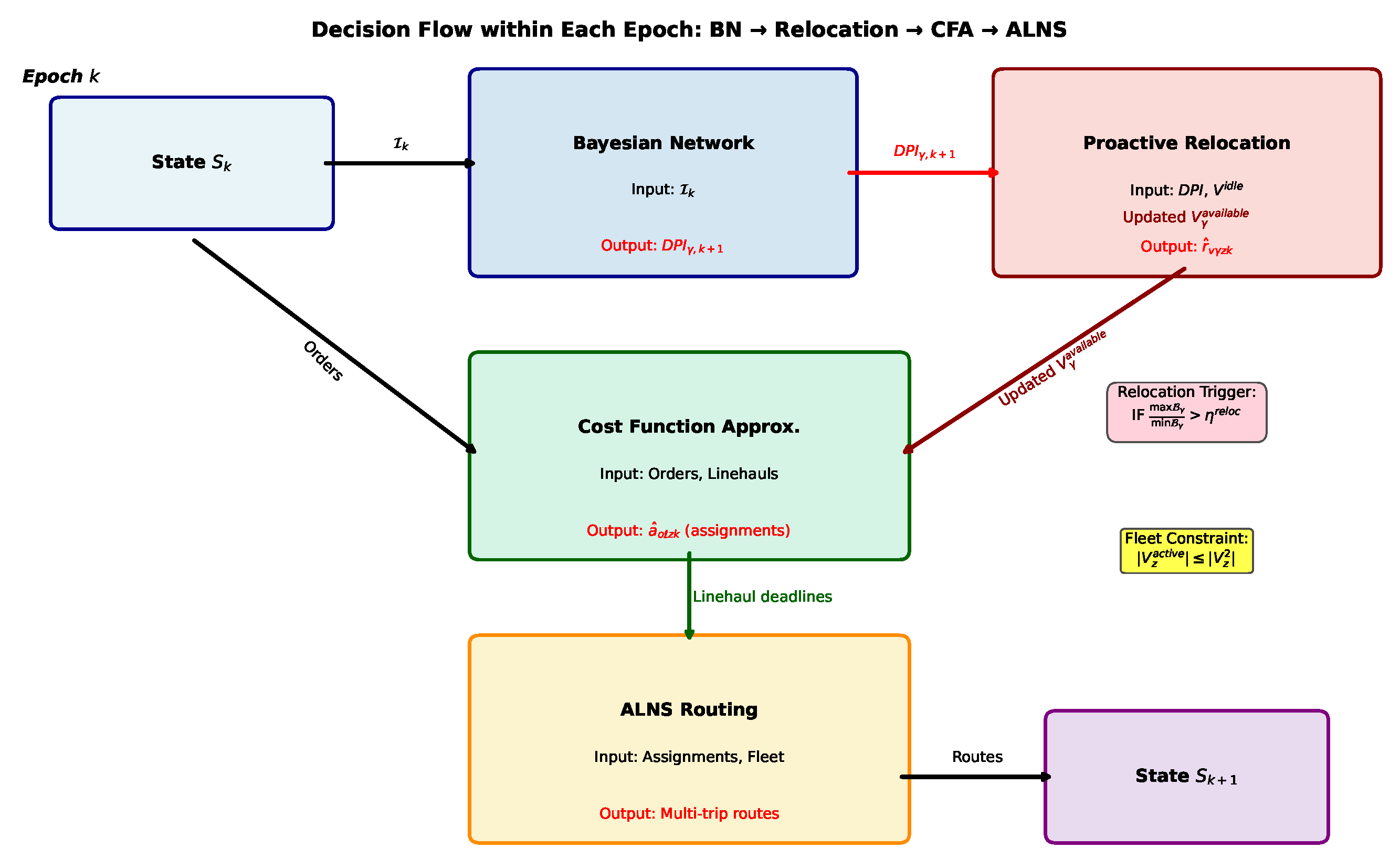
The MDP formulation of the FCMLP requires a solution approach that balances computational tractability with interpretable, proactive decision-making. Figure 1 illustrates the overall system architecture integrating predictive analytics (Bayesian Network, BN) with operational optimization (CFA and ALNS) to support proactive fleet management and efficient multi-trip routing under hard fleet constraints. Figure 2 depicts the integrated decision process within each epoch: the BN predicts spatial–temporal demand, vehicles are proactively relocated, and hierarchical optimization through CFA and ALNS determines order-to-linehaul assignments and two-echelon routes. This modular pipeline keeps real-time decisions computationally manageable while grounding them in transparent predictions.
We use a Bayesian Network for demand prediction because it provides interpretable conditional dependencies that operators can inspect and adjust, while naturally representing prediction uncertainty through probability distributions. The Cost Function Approximation (CFA) of Zamal et al. [27] enables real-time order-to-linehaul decisions by decomposing the stochastic problem into tractable deterministic subproblems parameterized by a few policy coefficients. Adaptive Large Neighborhood Search (ALNS) is adopted for routing due to its robustness on rich VRP variants and its destroy-and-repair paradigm, which is well suited to exploring trip consolidation and reassignment opportunities in multi-trip, two-echelon settings.
Overall, our approach consists of four interconnected components: (i) an interpretable BN for demand prediction using side information, (ii) a proactive vehicle relocation strategy driven by predicted demand imbalances, (iii) a CFA-based policy for dynamic order-to-linehaul assignment, and (iv) an ALNS-based solver for two-echelon routing with multi-trip operations under dynamically adjusted fleet distributions. The remainder of this section details these components and their interactions within the MDP framework.

4.1. Demand Prediction and Proactive Vehicle Relocation

This section presents our approach for leveraging side information through an interpretable Bayesian Network to predict demand patterns and make proactive relocation decisions. This predictive-proactive framework represents the key innovation that transforms reactive fleet management into anticipatory resource allocation.

4.1.1. Bayesian Network for Demand Prediction

We employ a Bayesian Network (BN) to model the probabilistic dependencies between side information and future demand patterns at each satellite.
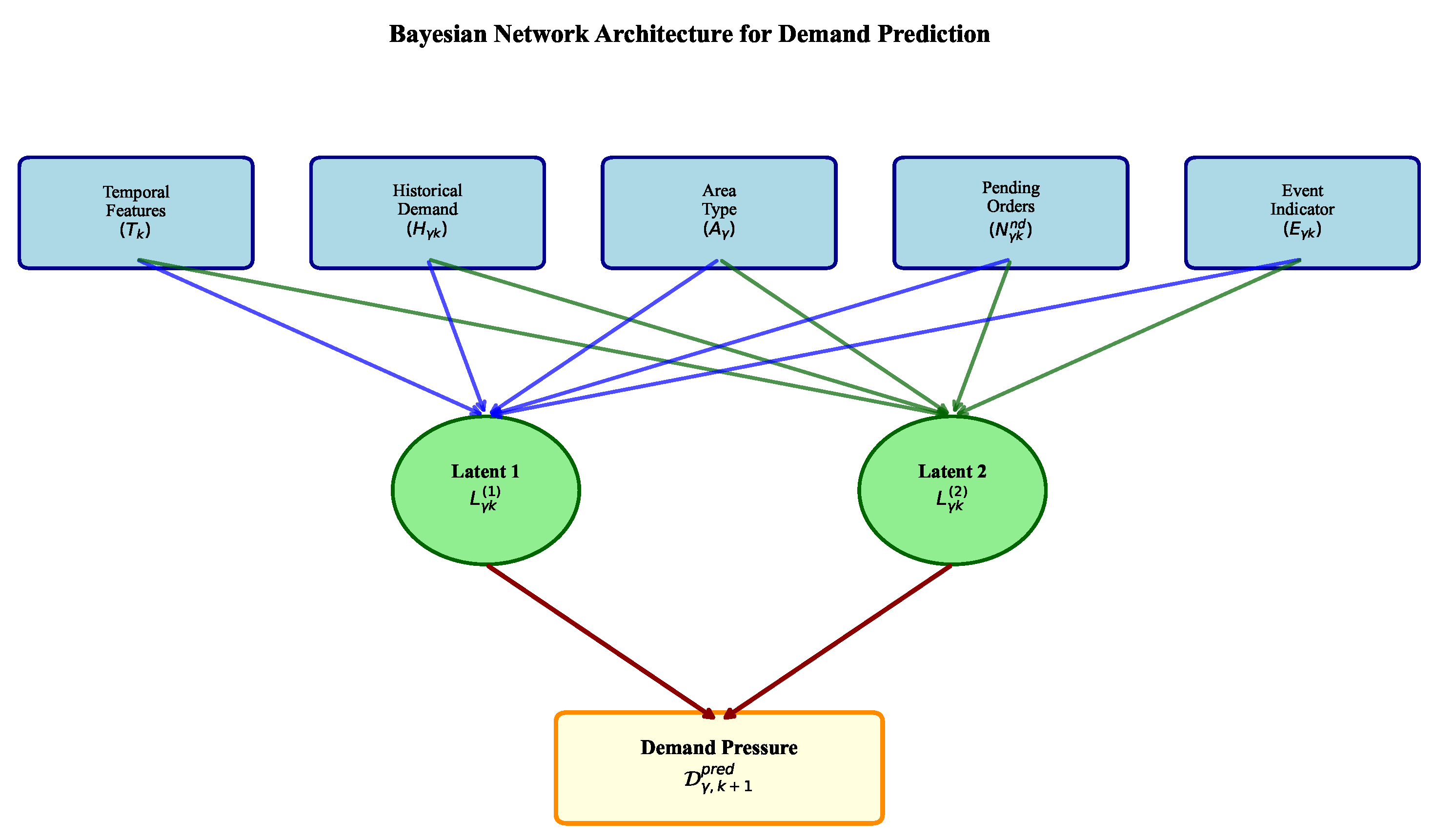
As shown in Figure 3, the network uses a three-layer hierarchical architecture with observable variables (temporal features, historical demand, area type, pending orders, and event indicators) as inputs, two latent variables capturing abstract demand drivers, and predicted demand pressure levels as outputs. The network parameters are learned from historical data using maximum likelihood estimation with Laplace smoothing.
For operational decision-making, the probabilistic output is converted into a continuous Demand Pressure Index (DPI),
DPI γ , k + 1 = κ L · P ( D γ , k + 1 pred = Low ) + κ M · P ( D γ , k + 1 pred = Medium ) + κ H · P ( D γ , k + 1 pred = High )
where weights κ L = 0.2 , κ M = 0.5 , and κ H = 0.8 reflect the relative operational impact of each demand level. The BN provides interpretability through influence analysis and contrastive explanations, enabling operators to understand and trust the relocation decisions. Full technical details, including the probability model, parameter learning procedures, and interpretability mechanisms, are provided in Supplementary Materials S2.

4.1.2. Proactive Relocation Strategy

Based on BN predictions, we implement a threshold-based relocation strategy that balances responsiveness with stability. At each decision epoch k, the strategy evaluates demand-supply imbalances and triggers relocations when beneficial.
Demand-Supply Imbalance Metric: For each satellite γ , we compute the predicted imbalance
B γ k = DPI γ , k + 1 max ( | V γ available | , 1 )
where | V γ available | is the number of idle vehicles currently at satellite γ .
System-Wide Imbalance Assessment: We evaluate the system-wide demand distribution to identify relocation opportunities
Imbalance Ratio = max γ G z B γ k min γ G z B γ k
Relocation is triggered when this ratio exceeds the threshold η reloc .
Relocation Optimization: When triggered, vehicles are relocated to minimize the expected system imbalance while accounting for relocation costs
min v V z idle γ G z c z var · d i s t ( γ v current , γ ) ξ · Δ B γ ( v ) · r ^ v γ z k
where Δ B γ ( v ) represents the improvement in system-wide imbalance from relocating vehicle v to satellite γ ,
Δ B γ ( v ) = B γ k DPI γ , k + 1 | V γ available | + 1 + B γ v current , k DPI γ v current , k + 1 max ( | V γ v current available | 1 , 1 )
Subject to operational constraints,
γ G z r ^ v γ z k 1 , v V z idle ( each vehicle relocated at most once )
| V γ available | v : γ v current = γ γ γ r ^ v γ z k ν , γ G z ( minimum service level )
t k + d i s t ( γ v current , γ ) speed t v next , v , γ : r ^ v γ z k = 1 ( time feasibility )
Explanation Generation: Each relocation decision is accompanied by an interpretable explanation as follows:
“Vehicle V12 relocated from Satellite A to Satellite B because of the following:
  • Predicted demand at B is HIGH (78% confidence) due to evening residential deliveries and 2 pending next-day orders.
  • Satellite B has only 2 available vehicles vs. predicted need for 5–6.
  • Satellite A has LOW predicted demand (82% confidence) with 4 excess vehicles.
  • Relocation distance 12 km, arrival before 14:30 peak period.”

4.1.3. Initial Fleet Distribution

At the beginning of the planning horizon ( k = 0 ), vehicles must be allocated across satellites to provide balanced coverage. The initial distribution considers both residual next-day orders from the previous operational period and historical demand patterns
| V γ 2 ( 0 ) | = | V z 2 | · w nd · N γ nd + w hist · H ¯ γ base γ G z ( w nd · N γ nd + w hist · H ¯ γ base ) + ϵ γ
where the following apply:
  • N γ nd represents pending next-day orders at satellite γ .
  • H ¯ γ base is the historical average morning demand for the satellite.
  • w nd = 0.7 and w hist = 0.3 are weights prioritizing immediate needs over historical patterns.
  • ϵ γ { 0 , 1 } allocates remaining vehicles after floor operation to highest-priority satellites.
This initial distribution ensures that the total fleet size constraint γ G z | V γ 2 ( 0 ) | = | V z 2 | is satisfied while providing coverage aligned with anticipated demand patterns.

4.2. Cost Function Approximation for Linehaul Assignment

At each decision epoch k, we assign orders o z k l = o z k fm o z k mm to available linehauls using a parameterized Mixed Integer Programming (MIP) formulation, known as Cost Function Approximation (CFA), where the city index z is now explicitly included to denote city-specific order sets (extending the notation o k l from Section 3). Here, o z k fm represents first-mile orders awaiting pickup in city z at epoch k, and o z k mm represents middle-mile orders already at the hub awaiting linehaul assignment. The CFA approach focuses on middle-mile transportation between city hubs, anticipating the effectiveness of vehicle routing operations that occur before and after linehaul transport.
To enable effective coordination between linehaul assignment and vehicle routing, we define several critical time points for each order. The latest delivery start time ( t o ldst ) represents when a vehicle must depart from the destination hub to meet the delivery time window, accounting for travel to the satellite, reload time, and final delivery. The latest linehaul departure time ( t o lldt ) identifies the last feasible linehaul that can deliver the order on time. For first-mile orders assigned to specific linehauls, the latest and earliest pickup start times ( t o lpst and t o epat ) determine the temporal constraints for pickup operations, considering synchronization requirements and time windows. These temporal concepts, formally defined in Supplementary Materials S2, establish the feasibility boundaries for order-to-linehaul assignments and subsequent routing decisions.
To capture the spatial and temporal variations in our dynamic system, we extend the notation from Section 3 to include city and time indices where appropriate. For instance, the linehaul capacity Q is extended to Q z k to reflect potential capacity variations across different cities z and time epochs k. Similarly, fixed costs F and variable costs U become F z k and U z k , and order weights q o become q o z k to account for city-specific and time-dependent characteristics. This notation extension allows us to model the heterogeneous operational conditions across different cities and time periods in the metropolitan logistics network.

4.2.1. Modified Assignment Cost with Slack Time

The concept of slack time is introduced to represent the temporal flexibility available for first-mile pickup and last-mile delivery operations. Slack time represents the buffer between when an order could theoretically complete its pickup/delivery operations and when it must complete them to meet linehaul schedules and customer time windows. Greater slack time provides more routing flexibility in both origin and destination cities, which can help reduce time window violations and the need for emergency vehicle deployments.
For each order o assigned to linehaul departing at time t ^ o , we define origin slack as the time buffer at the origin hub and destination slack as the time buffer at the destination hub. The modified assignment cost incorporating slack time is then given by
c ˜ o z k c f a = q o z k U z k α [ ( s o origin ) ε + ( s o dest ) ε ]
where q o z k is the weight of order o in city z at epoch k, U z k is the cost per unit weight for linehaul in city z at epoch k, α 0 is a weight parameter controlling the importance of slack time, ε 1 is an exponent that modulates the impact of slack time, and s o origin and s o dest represent the origin and destination slack times, respectively (detailed calculations in Supplementary Materials S2). When α = 0 , we recover pure cost minimization. Positive values of α encourage assignments that provide more operational flexibility for routing.

4.2.2. Deterministic Assignment Formulation

The linehaul assignment problem at epoch k is formulated as
min z Z L z k F z k w ^ z k + o o z k l L z k c ˜ o z k c f a a ^ o z k
s . t . o o z k l q o z k a ^ o z k Q z k w ^ z k , L z k , z Z
L ˜ o z k a ^ o z k = 1 , o o z k l , z Z
a ^ o z k , w ^ z k { 0 , 1 }
where F z k is the fixed cost for utilizing linehaul in city z at epoch k, w ^ z k is a binary variable indicating whether linehaul is utilized in city z at epoch k, a ^ o z k is a binary variable for order-to-linehaul assignment, Q z k is the capacity of linehaul in city z at epoch k, and L ˜ o z k L z k represents the subset of time-feasible linehauls for order o.
This deterministic formulation balances immediate costs with the temporal flexibility needed for efficient vehicle routing operations, improving overall system performance while maintaining computational tractability.

4.3. Parameterized Adaptive Large Neighborhood Search

This section presents our solution approach for the vehicle routing component of the FCMLP. The routing decisions must be made in real-time at each decision epoch k, taking as input the linehaul assignments determined by the CFA module and producing executable vehicle routes that respect fleet constraints and enable multi-trip operations.
The interface between the CFA and routing modules is carefully designed to maintain computational tractability while ensuring operational feasibility. The CFA module provides two critical inputs to the routing algorithm: (1) the assignment decisions a ^ o z k that specify which orders are assigned to which linehauls, and (2) the implied deadlines for first-mile pickups based on the assigned linehaul departure times. These assignments establish hard constraints that the routing algorithm must respect, creating a hierarchical decision structure where tactical linehaul decisions guide operational routing decisions.
Throughout this section, we maintain the city-specific and time-specific notation introduced in the CFA formulation. For instance, operational parameters such as linehaul capacities are denoted as Q z k rather than Q , reflecting the heterogeneous operational conditions across different cities and time periods in the metropolitan logistics network. Additionally, we define the ready-for-routing order set o z k R as a subset of orders requiring immediate routing attention, with the specific selection criteria detailed in the dispatching policy.

4.3.1. Algorithm Overview and Positioning

We employ a parameterized Adaptive Large Neighborhood Search (ALNS) algorithm triggered at each decision epoch to solve the fleet-constrained two-echelon vehicle routing problem with multi-trip operations. Extending Zamal et al. [18]’s static framework and building upon Zamal et al. [27]’s dynamic order assignment principles, we incorporate a parameterized dispatching policy where parameter β controls route planning activation timing, balancing routing efficiency with service responsiveness throughout the planning horizon.
The ALNS operates within our broader Markov Decision Process (MDP) framework, serving as the routing optimization module. At each decision epoch k, the algorithm receives a set of orders o z k R that have been deemed ready for routing based on the dispatching policy. These orders may include both first-mile pickups and last-mile deliveries, with their linehaul assignments (and corresponding deadlines) already determined by the Cost Function Approximation (CFA) module described in Section 4.2. The integration of multi-trip capabilities allows our ALNS to maximize fleet utilization under the hard constraint of limited vehicle availability.
Before executing the ALNS algorithm, the dynamic order data undergoes preprocessing to transform it into a static problem instance suitable for optimization. This conversion normalizes all temporal data relative to the current decision epoch t k , ensuring that each ALNS execution begins at time t = 0 while maintaining consistency with the broader dynamic system. The detailed preprocessing steps are provided in Supplementary Materials S2.

4.3.2. Parameterized Dispatching Policy

The dispatching policy determines which orders from the system state should be included in the ready-for-routing set o z k R at each decision epoch. This policy operates on the post-relocation fleet distribution, ensuring that routing decisions account for the proactively positioned vehicles. The policy is governed by a core parameter β , which represents a time buffer threshold.
o z k R = { o o z k : min ( t o lpst t k , t o ldst t k ) < β }
where t o lpst and t o ldst are the latest pickup start time and latest delivery start time defined in Section 4.2. The dispatching mechanism is thus triggered if there exists at least one order satisfying this temporal urgency criterion.
Small β values dispatch only urgent orders with limited routing flexibility, while large values enable frequent dispatching with greater consolidation opportunities. When regular fleet routing fails, emergency vehicles ensure service commitments at significantly higher cost, incentivizing efficient regular routing.
The dispatching policy operates on the post-relocation fleet distribution, ensuring that routing decisions account for the proactively positioned vehicles. Vehicles marked as “relocating” (i.e., s t a t u s v = relocating ) are excluded from the available vehicle set until their relocation completes at t v avail . This temporal coordination ensures that routing decisions are based on accurate vehicle availability.
The value of β interacts with the relocation decisions: aggressive relocation (low η r e l o c ) pairs well with conservative dispatching (high β ) to allow relocated vehicles time to reach their destinations, while conservative relocation (high η r e l o c ) can accommodate aggressive dispatching (low β ) since vehicles remain near their original positions. This interaction is captured in our hierarchical Bayesian optimization framework.

4.3.3. Core ALNS Framework

The ALNS follows a standard destroy-and-repair framework adapted for fleet-constrained multi-trip operations. The algorithm employs both small and large destroy operations, with small operations focused on local improvements and large operations for diversification. In each iteration, a destroy operator removes a subset of customers from the current solution, followed by a repair operator that reinserts these customers while respecting operational constraints.
The algorithm incorporates a three-tier hierarchy for customer insertion: (1) insertion into available vehicles, (2) creation of new trips for active vehicles if feasible, and (3) use of emergency vehicles as a last resort. This hierarchy ensures maximum utilization of the regular fleet before resorting to expensive emergency options. The acceptance mechanism employs simulated annealing with geometric cooling, balancing exploration and exploitation throughout the search process.
The objective function minimizes the total operational cost
f ( s o l ) = z Z r R z k 1 c r + v V z active c R v + c z fleet · | V z active | + o O k violated c o emergency
where c r denotes the total routing cost for route r and c R v represents the total routing cost for vehicle v across all its trips.
For multi-trip second-echelon routes, the route cost c R v for vehicle v includes all trip-specific components
c R v = i = 1 m v j = 1 n i d i s t h j 1 i , h j i · c z var + d i s t h n i i , γ v i · c z var
where d i s t i , j denotes the distance between locations i and j.
Large destroy operations result in unconditional acceptance to ensure diversification, while the standard simulated annealing mechanism balances exploitation and exploration throughout the search process.
The complete set of destroy operators (10 variants) and repair operators (8 variants), along with their detailed implementation, data structures for multi-trip representation, and parameter settings, are provided in Supplementary Materials S2. The algorithm’s integration with the dynamic system ensures that each static optimization contributes to the overall dynamic objectives while maintaining computational tractability for real-time operations.

4.4. Hierarchical Bayesian Optimization for Fleet Sizing and Operational Parameters

The joint optimization of fleet sizes and operational parameters presents a challenging mixed-integer stochastic optimization problem. We develop a hierarchical Bayesian optimization framework that decomposes the problem into strategic fleet sizing at the outer level and operational parameter tuning at the inner level.

4.4.1. Problem Decomposition

Let x = ( V 2 , χ ) denote the complete decision vector, where V 2 = ( | V 1 2 | , | V 2 2 | , , | V | Z | 2 | ) represents the fleet sizes and χ = ( α , β , ε , η r e l o c , ξ ) denotes the operational parameters. The objective function can be expressed as
f ( x ) = f ( V 2 , χ ) = z Z c z fixed · | V z 2 | + E [ C operational ( χ | V 2 ) ]
This structure suggests a hierarchical optimization
V 2 * = arg min V 2 V z Z c z fixed · | V z 2 | + min χ X E [ C operational ( χ | V 2 ) ]

4.4.2. Outer Level: Fleet Size Optimization

At the outer level, we model the minimum achievable total cost for each fleet configuration as a Gaussian Process. The next fleet configuration is selected by maximizing the Probability of Improvement (PI) acquisition function.

4.4.3. Inner Level: Operational Parameter Optimization

For each fleet configuration V 2 , we optimize operational parameters using standard Bayesian optimization with normalized parameter space and PI acquisition function.

4.4.4. Knowledge Transfer Mechanism

A key advantage of the hierarchical framework is the ability to transfer knowledge between similar fleet configurations. When initiating the inner optimization for a new fleet configuration V new 2 , we leverage the optimization history from previously evaluated configurations.
For each previously evaluated configuration V j 2 with optimal parameters χ j * , we compute a similarity weight
w j = exp ς z Z | V z , new 2 | | V z , j 2 | Δ z 2
where ς controls the influence decay rate and Δ z normalizes the fleet size differences. The initial parameter estimate for the new configuration is:
χ init = j w j χ j * j w j
This warm-start strategy significantly reduces the number of inner iterations required for convergence.

4.4.5. Implementation Details

The hierarchical optimization alternates between outer (10–15 iterations) and inner levels (15–25 evaluations each), with each configuration evaluated using M = 10 simulation runs. Early iterations use fewer inner evaluations for rapid exploration, while later iterations refine promising configurations, ensuring efficient convergence within practical computational limits.

5. Computational Experiments

This section presents computational experiments to evaluate the performance of our fleet-constrained metropolitan logistics problem (FCMLP) framework. We assess the effectiveness of multi-trip operations under fleet constraints and analyze the trade-offs between fleet size, operational costs, and service quality through both controlled simulation experiments and real-world case studies. Particular emphasis is placed on evaluating the impact of our Bayesian Network-based demand prediction and proactive vehicle relocation strategies.

5.1. Experimental Setup

We implement our solution framework in Python and conduct all computational experiments on a system with an AMD Ryzen 5 5600X 6-Core Processor (3.70 GHz) and 16 GB of RAM. For solving the mixed-integer programming formulations in our Cost Function Approximation module, we employ IBM ILOG CPLEX 22.1.1.0 as the optimization solver. All code is implemented in Python 3.9 with NumPy for numerical computations and multiprocessing libraries for parallel simulation runs. The datasets are available in GitHub repository: https://github.com/xyyao1116/FCMLP (accessed on 24 November 2025).

5.1.1. System Configuration and Test Instances

We construct a metropolitan logistics network comprising interconnected cities, each with one central hub at coordinates (50, 50) and two satellites positioned 20–30 units away in opposite directions on a 100 × 100 UTM grid. This two-echelon architecture balances consolidation efficiency with last-mile delivery flexibility.
The system operates over a 10 h planning horizon (600 min) divided into 10 hourly decision epochs. Orders arrive uniformly with weights between one and four units and differentiated service commitments: same-day orders require pickup within 3 h and delivery 2–5 h after arrival, while next-day orders allow pickup until minute 420 and concentrated morning delivery (540–600 min). Daily order volume ranges from 150 to 200 per city.
Vehicle fleets operate with distinct capacities: first-echelon vehicles (75 units) shuttle between hubs and satellites with unlimited availability, while second-echelon vehicles (10 units) handle urban delivery with fleet size as a decision variable. Operations include 15 min satellite reload times and 5 min customer service times, with trips capped at 180 min.
The linehaul system incorporates temporal variations: peak hours (0–120, 480–600 min) reduce capacity to 80% and increase costs/travel times to 120%; off-peak hours (240–360 min) expand capacity to 120% with 80% costs/times; regular hours maintain baseline parameters. This captures metropolitan freight dynamics without demand-based adjustments.
Cost parameters reflect operational realities: regular vehicles incur 150 units daily fixed cost plus 2 units/km variable cost; emergency deployments cost 500 units fixed plus 5 units/km variable. These differentials drive the fleet size versus emergency deployment trade-off. Table 2 summarizes all configuration parameters.

5.1.2. Experimental Design

We conduct experiments in two phases. Phase 1 employs controlled simulations using a 2 × 3 factorial design with hub configurations (two or three hubs) and demand scenarios: More Next-Day (MND: 25% same-day, 75% next-day), Balanced (BAL: 50–50%), and More Same-Day (MSD: 75% same-day, 25% next-day). Phase 2 validates our framework using 14 days of operational data from a major e-commerce platform in Jakarta, comparing against their current Latest Departure Schedule (LDS) heuristic.

5.1.3. Solution Methods

We compare three variants to isolate the impact of our contributions:
OF-ST (Optimized Fleet, Single-Trip): Adapts Zamal et al. [27]’s framework by adding fleet constraints while restricting vehicles to single trips. This baseline jointly optimizes fleet size and operational parameters ( α , β , ε ) without multi-trip capabilities.
OF-MT (Multi-Trip): Enables multi-trip operations with the same optimization framework, allowing vehicles to perform multiple delivery cycles.
OF-MT-R (Multi-Trip with Relocation): Adds Bayesian Network demand prediction and proactive vehicle relocation to OF-MT, using the same fleet size but repositioning idle vehicles based on predicted demand.
All methods use identical Bayesian optimization with 10 iterations evaluating 30-day simulations each. The hierarchical framework optimizes fleet sizes | V z 2 | [ 10 , 30 ] and operational parameters: slack weight α [ 0 , 1 ] , dispatching threshold β [ 30 , 180 ] min, slack exponent ε [ 1 , 3 ] , and relocation threshold η reloc [ 1.5 , 4.0 ] and balance weight ξ [ 0.5 , 2.0 ] for OF-MT-R only. All methods use a Probability-of-Improvement acquisition function, initialized with a small random design.

5.2. Simulation Results

5.2.1. Overall Performance Comparison

Table 3 summarizes the optimized fleet sizes and total costs across all test instances, highlighting the systematic advantages of multi-trip operations and the incremental benefits of proactive relocation.
The results reveal substantial performance improvements through multi-trip operations, with further gains from proactive relocation. Across all scenarios, OF-MT achieves an average fleet reduction of 22.6% (from 64.3 to 49.8 vehicles) while reducing total costs by 20.5%. The addition of proactive relocation in OF-MT-R, while maintaining the same fleet size as OF-MT, delivers an additional 6.7% cost reduction and reduces emergency rates from 6.5% to 5.2% on average.
The cost reduction pattern varies with demand characteristics. MSD scenarios show the highest absolute cost improvements, while the relative benefit of relocation is most pronounced in BAL scenarios, where the mix of same-day and next-day orders creates more complex demand patterns that benefit from anticipatory positioning. The average daily relocation frequency increases with same-day demand proportion, ranging from 3.2 to 4.5 relocations in MND scenarios and 8.4 to 10.3 in MSD scenarios, reflecting the greater spatial-temporal variability in urgent delivery requirements.

5.2.2. Impact of Proactive Relocation

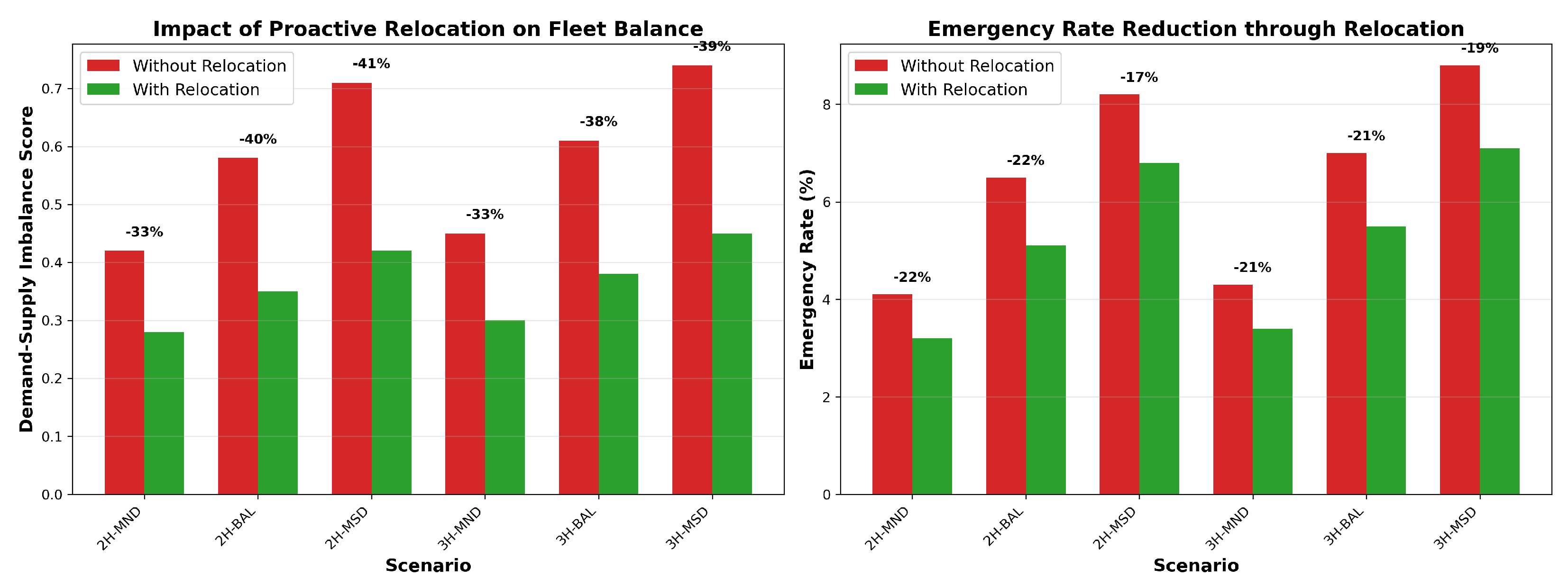
Figure 4 illustrates the effectiveness of proactive relocation in balancing fleet distribution and reducing emergency vehicle deployments across different scenarios. Left panel shows the average standard deviation of demand-supply imbalance scores across satellites. Right panel displays the percentage of orders requiring emergency vehicles. Percentages above bars indicate the relative improvement achieved through relocation.
The proactive relocation strategy demonstrates consistent effectiveness in reducing demand-supply imbalances across all scenarios. Without relocation (OF-MT), the imbalance scores range from 0.42 to 0.75, indicating significant disparities in vehicle availability relative to demand across satellites. The implementation of BN-based prediction and proactive relocation (OF-MT-R) reduces these imbalances by 33–41%, with the most substantial improvements observed in MSD scenarios where demand patterns are most volatile.
The reduction in imbalance directly translates to improved service reliability. Emergency rates decrease by 17–22% across all scenarios when relocation is enabled, with the largest absolute reductions occurring in high-demand scenarios. This improvement stems from the system’s ability to anticipate demand surges and preposition vehicles accordingly, reducing instances where local fleet capacity is overwhelmed. The effectiveness is particularly notable given that no additional vehicles are added—the same fleet size achieves superior performance through better spatial distribution.

5.2.3. Fleet Reduction Analysis

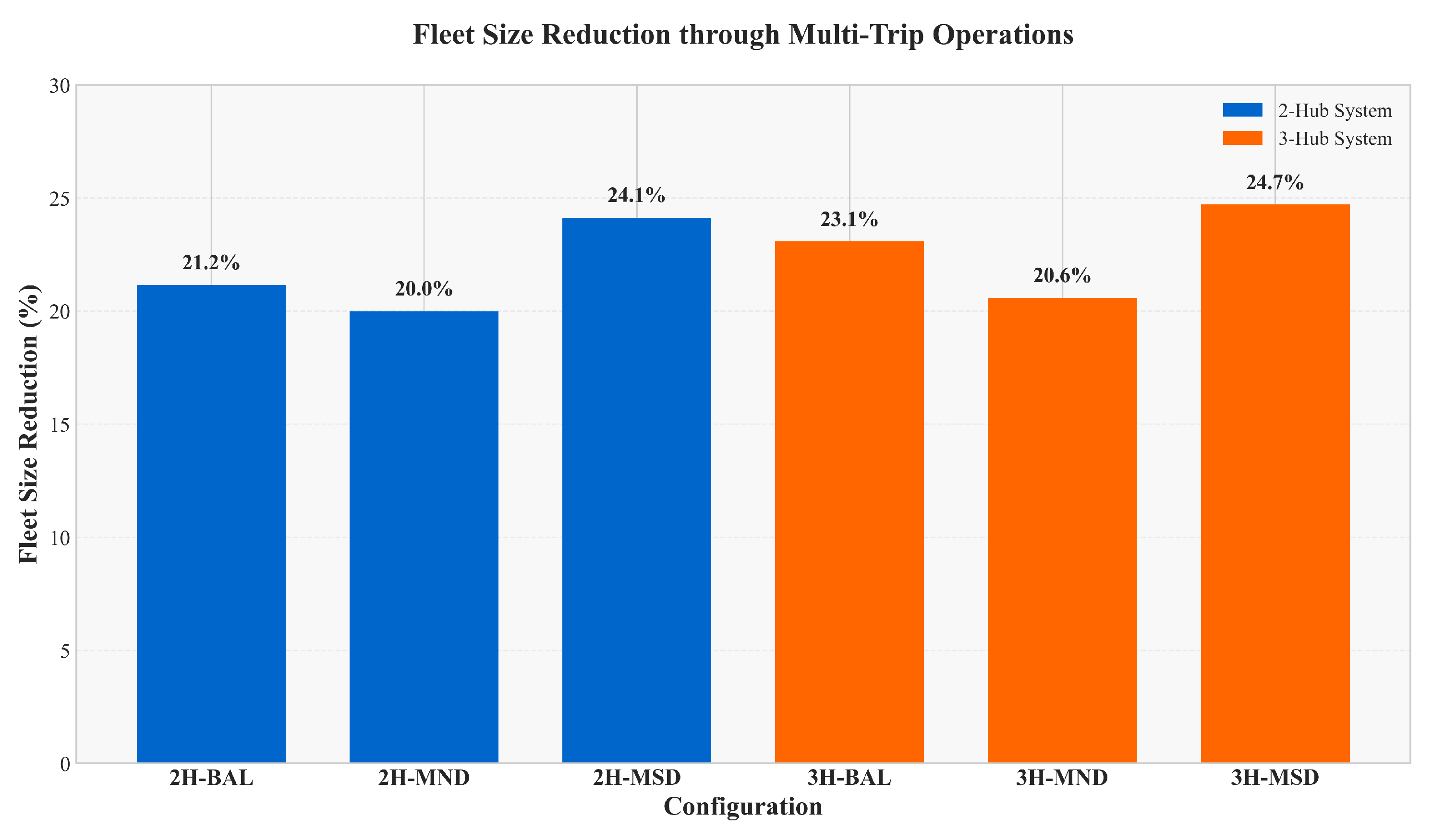
Figure 5 illustrates the fleet size reduction achieved through multi-trip operations across different demand scenarios.
The fleet reduction pattern exhibits clear demand dependency. MSD scenarios achieve the highest fleet reductions (24.1% for 2-hub, 24.7% for 3-hub), as the urgency of same-day deliveries aligns well with the increased vehicle circulation enabled by multi-trip operations. Conversely, MND scenarios show smaller reductions (20.0% for 2-hub, 20.6% for 3-hub), as next-day orders’ concentrated morning delivery windows limit opportunities for vehicle reuse. The consistent reduction across different hub configurations suggests that multi-trip benefits are robust to network scale variations.

5.2.4. Cost Structure Analysis

Table 4 decomposes the total cost savings into component categories, revealing how multi-trip operations and proactive relocation impact different cost drivers.
The cost decomposition reveals several key insights. Routing costs dominate the total (67.1–81.0%), making their reduction through efficient operations particularly impactful. The introduction of proactive relocation (OF-MT-R) reduces routing costs by an additional 2.3–3.9% compared to OF-MT, demonstrating that better vehicle positioning leads to shorter travel distances. Emergency costs show the most dramatic improvement with relocation, decreasing by 27–32% relative to OF-MT. While relocation incurs additional costs (averaging 670–2147 units across scenarios), these are vastly outweighed by the savings in emergency deployments and routing efficiency. The combined linehaul and relocation costs in OF-MT-R remain below 3.5% of total costs across all scenarios, confirming the economic viability of the proactive strategy.

5.2.5. Relocation Pattern Analysis

Table 5 provides detailed insights into the temporal distribution and effectiveness of proactive relocations throughout the operational day.
The temporal analysis reveals sophisticated relocation patterns aligned with demand dynamics. Afternoon periods (200–400 min) consistently show the highest relocation frequency across all scenarios, coinciding with the preparation for evening delivery peaks. The Bayesian Network demonstrates robust predictive performance with accuracy ranging from 72.5% to 87.1%, with higher accuracy in afternoon periods when demand patterns are more established. Notably, BN accuracy improves with demand complexity—MSD scenarios achieve 4–8% higher accuracy than MND scenarios, suggesting that the model effectively learns from the richer spatial-temporal patterns in same-day heavy operations.
Cost savings from relocations show a clear correlation with both relocation frequency and BN accuracy. Each relocation generates average savings of 1500–2000 cost units, with higher values in complex demand scenarios. The return on investment is substantial: relocation costs average 100–150 units per move, yielding benefit–cost ratios exceeding 10:1 in all scenarios.

5.2.6. Temporal Relocation Patterns

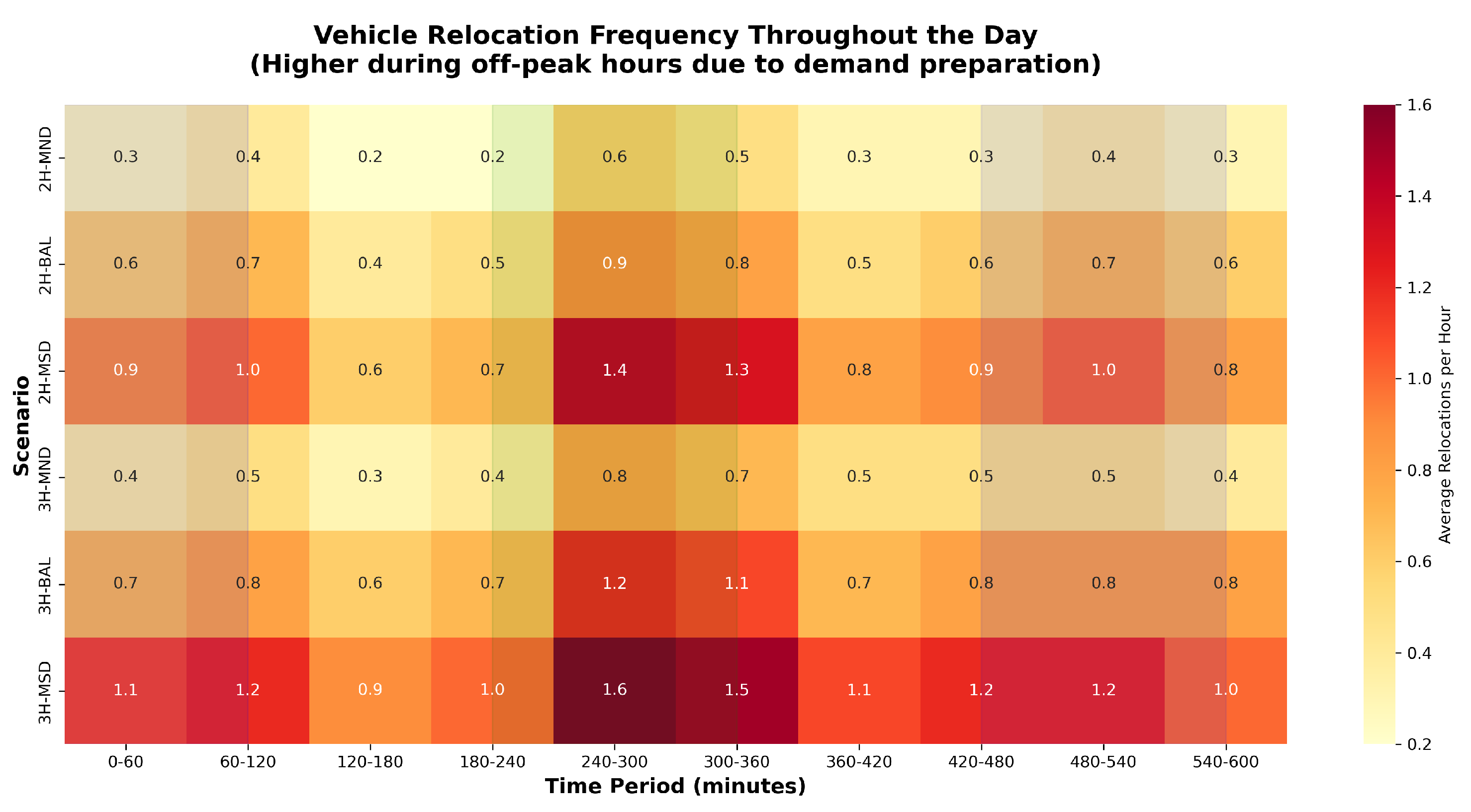
Figure 6 visualizes the hourly distribution of vehicle relocations across different scenarios and time periods, revealing how the system adapts its proactive positioning strategy to anticipated demand patterns.
The heatmap reveals distinct temporal patterns in relocation activity. The most intense relocation periods occur during hours 240–360 (off-peak afternoon), when the system prepares for evening delivery rushes by repositioning vehicles from low-demand to high-demand satellites. MSD scenarios exhibit the highest relocation intensity (up to 1.6 relocations per hour), reflecting the continuous spatial rebalancing required for same-day deliveries. Conversely, MND scenarios show more concentrated relocation patterns, primarily during mid-day periods when preparing for next-morning deliveries. This temporal intelligence demonstrates the system’s ability to anticipate future demand based on historical patterns and current order flows.

5.2.7. Multi-Trip Utilization Patterns

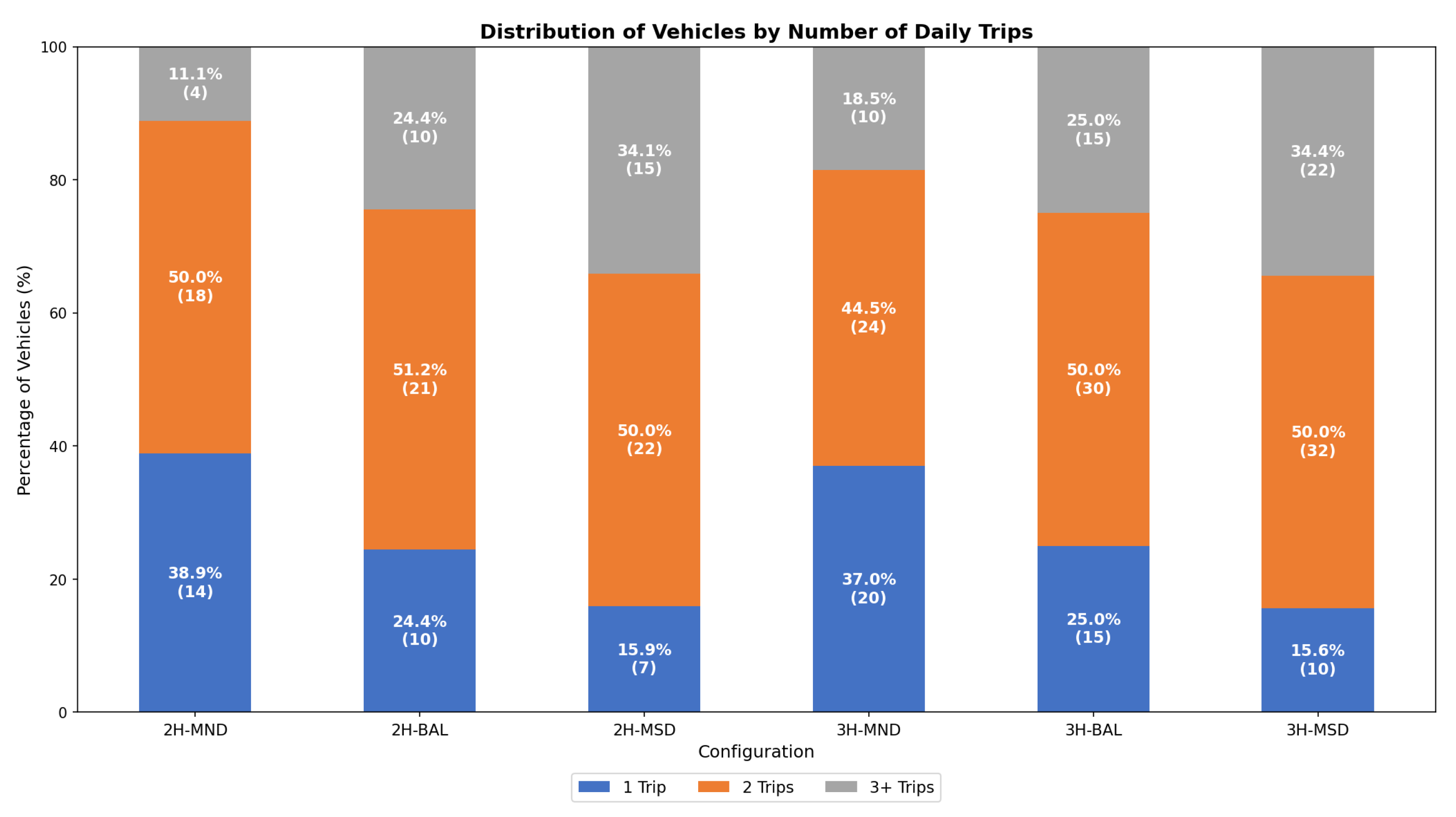
Figure 7 shows the distribution of vehicles by number of trips performed, demonstrating how the system leverages multi-trip capabilities under different operational conditions.
The trip distribution reveals how proactive relocation enhances multi-trip utilization. While OF-MT shows standard utilization patterns, OF-MT-R demonstrates a shift toward higher trip counts, particularly in the 3+ trip category. This improvement is most pronounced in BAL and MSD scenarios, where proactive positioning enables vehicles to capture additional delivery opportunities that would otherwise be missed due to poor initial positioning. The enhanced utilization contributes to the cost reductions observed in OF-MT-R without requiring additional vehicle resources.

5.2.8. Optimized Parameter Analysis

Table 6 presents the optimized operational parameters for each configuration, revealing how the system adapts to different demand patterns and operational strategies.
The parameter optimization reveals systematic adaptations across different operational strategies. The relocation parameters in OF-MT-R show interesting patterns: the threshold η reloc decreases with demand complexity (3.2–3.5 for MND down to 2.0–2.2 for MSD), indicating more aggressive relocation in volatile environments. Conversely, the balance weight ξ increases with same-day proportion (0.7–0.8 for MND up to 1.1–1.2 for MSD), suggesting greater willingness to invest in repositioning when demand urgency is high. These parameter adaptations demonstrate the system’s ability to self-tune based on operational characteristics.

5.3. Sensitivity Analysis

Impact of Fleet Size on Operational Strategy

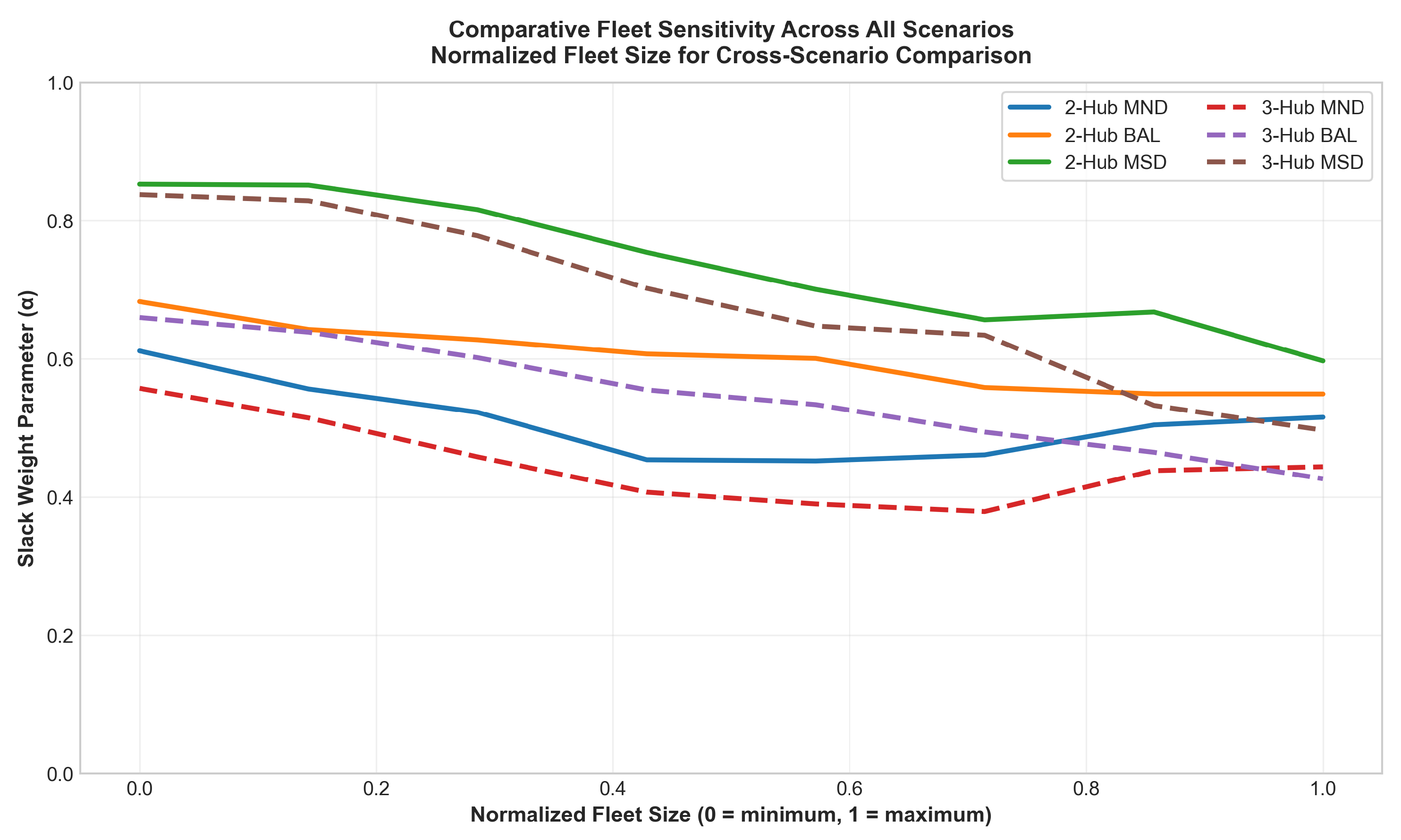
To understand the relationship between resource constraints and operational strategies, we analyze how the optimal slack weight parameter α varies with fleet size. Figure 8 illustrates this relationship across different operational modes.
The sensitivity analysis reveals an inverse relationship between fleet size and the importance of slack time in assignment decisions. As fleet size decreases from 30 to 10 vehicles per city, the optimal α value increases from approximately 0.4 to 0.8, indicating that constrained fleets require greater temporal flexibility to maintain service quality. This pattern is more pronounced for multi-trip operations (OF-MT and OF-MT-R), where the slope is steeper, suggesting that temporal coordination becomes critical when combining limited resources with vehicle reuse strategies. Notably, OF-MT-R shows the steepest slope, indicating that proactive relocation further amplifies the importance of temporal flexibility in resource-constrained environments.

5.4. Case Study

5.4.1. Dataset Description

We validate our approach using operational data from a major e-commerce platform’s logistics network in the Jakarta Metropolitan Area. To enable direct comparison with our simulation experiments, we organize the real-world data into the same 2 × 3 factorial design as follows:
  • Time period: 14 operational days.
  • Network configurations: 2-hub and 3-hub systems.
  • The demand scenarios are as follows:
    -
    More Next-Day (MND): 25% same-day, 75% next-day orders.
    -
    Balanced (BAL): 50% same-day, 50% next-day orders.
    -
    More Same-Day (MSD): 75% same-day, 25% next-day orders.
  • Order volume: 2000–3000 orders per configuration.
  • Current operation: Latest Departure Schedule (LDS) heuristic with predetermined fleet allocation.
Each hub configuration operates with co-located hub-satellite facilities, reflecting the common practice of integrating transshipment points with distribution centers in dense urban environments. The 2-hub system covers the central metropolitan area, while the 3-hub system extends coverage to peripheral regions. Order characteristics and operational parameters match those used in our simulation experiments, ensuring consistent evaluation conditions.

5.4.2. Performance Comparison

Table 7 compares our approaches against the company’s current system, demonstrating the practical impact of our optimization framework.
The real-world validation demonstrates even stronger performance improvements than simulation results. Our OF-MT-R approach maintains the same fleet size as OF-MT (39.1% reduction from current LDS) while achieving an additional 10.3% cost reduction through proactive relocation. Most significantly, emergency rates drop from 13.4% (LDS average) to 9.3% with OF-MT-R, a 42.8% reduction that substantially improves service reliability.
The superior real-world performance stems from several factors. The current LDS system operates with conservative rules that fail to exploit multi-trip opportunities and lacks dynamic adaptation to demand patterns. Real-world demand exhibits stronger spatial-temporal clustering than our uniformly distributed simulation demand, creating more opportunities for effective vehicle relocation. Additionally, the BN model effectively learns location-specific demand patterns from historical data, achieving prediction accuracies of 78–86% in the real-world setting compared to 72–87% in simulations.

6. Conclusions

This section synthesizes the key insights from our computational experiments and examines their implications for fleet-constrained metropolitan logistics. We analyze the performance drivers of our approach, assess its computational characteristics, and acknowledge the limitations that guide future research directions.

6.1. Key Findings

Our comprehensive experiments reveal four critical insights into fleet-constrained metropolitan logistics:
First, the integration of Bayesian Network-based demand prediction with proactive vehicle relocation delivers substantial operational improvements without requiring additional fleet resources. The OF-MT-R approach achieves 6.7% cost reduction and 20% emergency rate reduction compared to OF-MT in simulations, with even greater benefits (10.3% cost reduction, 21.2% emergency rate reduction) in real-world applications. These improvements demonstrate that predictive analytics can effectively substitute for physical assets in logistics operations.
Second, multi-trip operations deliver substantial efficiency gains when properly implemented, achieving 20.5% cost reduction and 22.6% fleet reduction in controlled simulations, with even greater improvements (49.5% cost reduction when combined with relocation) in real-world applications. These benefits stem from the fundamental synergy between two-echelon architecture and multi-trip strategies—satellites positioned near customer clusters dramatically reduce reload time compared to central depot returns, making multiple trips economically viable even under tight time constraints.
Third, the effectiveness of both multi-trip operations and proactive relocation exhibits strong demand dependency. Same-day heavy scenarios achieve the highest improvements, as urgent, continuously arriving orders create natural opportunities for vehicle circulation and benefit most from anticipatory positioning. The system demonstrates systematic adaptation through parameter tuning, with relocation thresholds decreasing and balance weights increasing as demand urgency rises. Our demand prediction analysis based on the interpretable Bayesian Network further reveals how temporal and spatial features jointly drive these improvements, providing a structured explanation for the observed performance differences across scenarios.
Fourth, successful implementation requires fundamental shifts in operational parameters and management philosophy. Our analysis shows that systems must increase emphasis on temporal flexibility, adopt earlier dispatching triggers, and embrace dynamic fleet distribution based on predictive insights. The interpretability of the Bayesian Network enables operators to understand and trust relocation decisions, facilitating the transition from reactive to proactive logistics management.

6.2. Computational Performance

Our framework demonstrates strong computational performance within metropolitan logistics operational constraints. The hourly decision epochs provide sufficient time for problem instances with 150–200 orders, with our implementation requiring 5–10 min. The hierarchical Bayesian optimization converges within 10–15 outer iterations, each inner optimization completing in under 25 evaluations. The modular architecture enables parallel processing across cities, meeting real-time requirements for typical operations, while larger networks may benefit from decomposition strategies.

6.3. Limitations and Future Directions

While our results demonstrate significant benefits, several limitations warrant acknowledgment. Our deterministic travel time assumption simplifies routing but may underestimate congestion impacts. The prohibition of split deliveries maintains operational simplicity but sacrifices potential efficiency gains. The fixed satellite assignment policy reflects practical constraints but reduces flexibility. Additionally, our Bayesian Network operates at satellite-level aggregation, which limits demand prediction granularity and may omit finer spatial patterns; finer-grained predictions could enable more precise positioning.
Future research could address these limitations through stochastic travel time modeling, relaxing split delivery constraints for specific order types, developing distributed optimization for larger networks, and enhancing demand prediction granularity through hierarchical or higher-resolution models to support more fine-grained relocation decisions. The modular architecture facilitates such extensions without restructuring the entire framework, providing a practical foundation for advancing fleet-constrained metropolitan logistics.

Supplementary Materials

The following supporting information can be downloaded at https://www.mdpi.com/article/10.3390/app152312609/s1, Supplementary Materials S1: Complete list of notation used in this paper; Supplementary Materials S2: Technical details including Bayesian Network implementation details and ALNS algorithm details.

Author Contributions

Conceptualization, M.L.; methodology, L.S.; software, X.Y.; validation, L.S.; writing—original draft, X.Y.; supervision, M.L. All authors have read and agreed to the published version of the manuscript.

Funding

This work was supported by the National Natural Science Foundation of China (NSFC) under Grant 72071144.

Institutional Review Board Statement

Not applicable.

Informed Consent Statement

Not applicable.

Data Availability Statement

The datasets used in this study are available at: https://github.com/xyyao1116/FCMLP (accessed on 24 November 2025).

Acknowledgments

The authors are grateful for the valuable comments from the editor and reviewers.

Conflicts of Interest

The authors declare that they have no known competing financial interests or personal relationships that could have appeared to influence the work reported in this paper.

References

  1. Sluijk, N.; Florio, A.M.; Kinable, J.; Dellaert, N.; Van Woensel, T. Two-echelon vehicle routing problems: A literature review. Eur. J. Oper. Res. 2023, 304, 865–886. [Google Scholar] [CrossRef]
  2. Cattaruzza, D.; Absi, N.; Feillet, D. Vehicle routing problems with multiple trips. Ann. Oper. Res. 2018, 271, 127–159. [Google Scholar] [CrossRef]
  3. Dumez, D.; Tilk, C.; Irnich, S.; Lehuédé, F.; Olkis, K.; Péton, O. A matheuristic for a 2-echelon vehicle routing problem with capacitated satellites and reverse flows. Eur. J. Oper. Res. 2023, 305, 64–84. [Google Scholar] [CrossRef]
  4. Lehmann, J.; Winkenbach, M. A matheuristic for the Two-Echelon Multi-Trip Vehicle Routing Problem with mixed pickup and delivery demand and time windows. Transp. Res. Part C Emerg. Technol. 2024, 160, 104522. [Google Scholar] [CrossRef]
  5. Hernandez, F.; Feillet, D.; Giroudeau, R.; Naud, O. Branch-and-price algorithms for the solution of the multi-trip vehicle routing problem with time windows. Eur. J. Oper. Res. 2016, 249, 551–559. [Google Scholar] [CrossRef]
  6. Zhen, L.; Ma, C.; Wang, K.; Xiao, L.; Zhang, W. Multi-depot multi-trip vehicle routing problem with time windows and release dates. Transp. Res. Part E Logist. Transp. Rev. 2020, 135, 101866. [Google Scholar] [CrossRef]
  7. Fermín Cueto, P.; Gjeroska, I.; Solà Vilalta, A.; Anjos, M.F. A solution approach for multi-trip vehicle routing problems with time windows, fleet sizing, and depot location. Networks 2021, 78, 503–522. [Google Scholar] [CrossRef]
  8. Chen, E.; Zhou, Z.; Li, R.; Chang, Z.; Shi, J. The multi-fleet delivery problem combined with trucks, tricycles, and drones for last-mile logistics efficiency requirements under multiple budget constraints. Transp. Res. Part E Logist. Transp. Rev. 2024, 187, 103573. [Google Scholar] [CrossRef]
  9. Karademir, C.; Beirigo, B.A.; Atasoy, B. A two-echelon multi-trip vehicle routing problem with synchronization for an integrated water- and land-based transportation system. Eur. J. Oper. Res. 2025, 322, 480–499. [Google Scholar] [CrossRef]
  10. Pan, B.; Zhang, Z.; Lim, A. Multi-trip time-dependent vehicle routing problem with time windows. Eur. J. Oper. Res. 2021, 291, 218–231. [Google Scholar] [CrossRef]
  11. Grangier, P.; Gendreau, M.; Lehuédé, F.; Rousseau, L.-M. An adaptive large neighborhood search for the two-echelon multiple-trip vehicle routing problem with satellite synchronization. Eur. J. Oper. Res. 2016, 254, 80–91. [Google Scholar] [CrossRef]
  12. Enthoven, D.L.J.U.; Jargalsaikhan, B.; Roodbergen, K.J.; uit het Broek, M.A.J.; Schrotenboer, A.H. The two-echelon vehicle routing problem with covering options: City logistics with cargo bikes and parcel lockers. Comput. Oper. Res. 2020, 118, 104919. [Google Scholar] [CrossRef]
  13. Li, H.; Wang, H.; Chen, J.; Bai, M. Two-echelon vehicle routing problem with satellite bi-synchronization. Eur. J. Oper. Res. 2021, 288, 775–793. [Google Scholar] [CrossRef]
  14. Dos Santos, A.G.; Viana, A.; Pedroso, J.P. 2-echelon lastmile delivery with lockers and occasional couriers. Transp. Res. Part E Logist. Transp. Rev. 2022, 162, 102714. [Google Scholar] [CrossRef]
  15. Dahimi, A.; Lurkin, V.; Mohammadi, M.; Van Woensel, T. A two-echelon vehicle routing problem with mobile satellites and multiple commodities. Eur. J. Oper. Res. 2025, 326, 124–140. [Google Scholar] [CrossRef]
  16. Tadaros, M.; Kyriakakis, N.A. A Hybrid Clustered Ant Colony Optimization Approach for the Hierarchical Multi-Switch Multi-Echelon Vehicle Routing Problem with Service Times. Comput. Ind. Eng. 2024, 190, 110040. [Google Scholar] [CrossRef]
  17. Gutierrez, A.; Labadie, N.; Prins, C. A Two-echelon Vehicle Routing Problem with time-dependent travel times in the city logistics context. EURO J. Transp. Logist. 2024, 13, 100133. [Google Scholar] [CrossRef]
  18. Zamal, M.A.; Schrotenboer, A.H.; Van Woensel, T. The two-echelon vehicle routing problem with pickups, deliveries, and deadlines. Comput. Oper. Res. 2025, 179, 107016. [Google Scholar] [CrossRef]
  19. Şahin, M.K.; Yaman, H. A Branch and Price Algorithm for the Heterogeneous Fleet Multi-Depot Multi-Trip Vehicle Routing Problem with Time Windows. Transp. Sci. 2022, 56, 1636–1657. [Google Scholar] [CrossRef]
  20. Guo, S.; Hu, H.; Xue, H. A Two-Echelon Multi-Trip Capacitated Vehicle Routing Problem with Time Windows for Fresh E-Commerce Logistics under Front Warehouse Mode. Systems 2024, 12, 205. [Google Scholar] [CrossRef]
  21. Crainic, T.G.; Gobbato, L.; Perboli, G.; Rei, W. Logistics capacity planning: A stochastic bin packing formulation and a progressive hedging meta-heuristic. Eur. J. Oper. Res. 2016, 253, 404–417. [Google Scholar] [CrossRef]
  22. Ghilas, V.; Demir, E.; Van Woensel, T. A scenario-based planning for the pickup and delivery problem with time windows, scheduled lines and stochastic demands. Transp. Res. Part B Methodol. 2016, 91, 34–51. [Google Scholar] [CrossRef]
  23. Klapp, M.A.; Erera, A.L.; Toriello, A. The Dynamic Dispatch Waves Problem for same-day delivery. Eur. J. Oper. Res. 2018, 271, 519–534. [Google Scholar] [CrossRef]
  24. Van Heeswijk, W.J.A.; Mes, M.R.K.; Schutten, J.M.J. The Delivery Dispatching Problem with Time Windows for Urban Consolidation Centers. Transp. Sci. 2019, 53, 203–221. [Google Scholar] [CrossRef]
  25. He, Y.; Hewitt, M.; Lehuédé, F.; Medina, J.; Péton, O. A continuous-time service network design and vehicle routing problem. Networks 2023, 83, 300–323. [Google Scholar] [CrossRef]
  26. Medina, J.; Hewitt, M.; Lehuédé, F.; Péton, O. Integrating long-haul and local transportation planning: The Service Network Design and Routing Problem. EURO J. Transp. Logist. 2019, 8, 119–145. [Google Scholar] [CrossRef]
  27. Zamal, M.A.; Schrotenboer, A.H.; Van Woensel, T. End-to-end logistics in metropolitan areas: A stochastic dynamic order-assignment and dispatching problem. Transp. Res. Part B Methodol. 2025, 199, 103249. [Google Scholar] [CrossRef]
  28. Sluijk, N.; Florio, A.M.; Kinable, J.; Dellaert, N.; Van Woensel, T. A Chance-Constrained Two-Echelon Vehicle Routing Problem with Stochastic Demands. Transp. Sci. 2023, 57, 252–272. [Google Scholar] [CrossRef]
  29. Cai, D.; Chen, K.; Lin, Z.; Li, D.; Zhou, T.; Leung, M.-F. JointSTNet: Joint Pre-Training for Spatial-Temporal Traffic Forecasting. IEEE Trans. Consum. Electron. 2025, 71, 6239–6252. [Google Scholar] [CrossRef]
  30. Beni Prathiba, S.; Ram Krishnamoorthy, S.; Soundari Kannan, K.; Selvaraj, A.K.; Ranganayakulu, D.; Fang, K.; Gadekallu, T.R. Digital Twin-Enabled Real-Time Optimization System for Traffic and Power Grid Management in 6G-Driven Smart Cities. IEEE Internet Things J. 2025, 12, 29164–29175. [Google Scholar] [CrossRef]
  31. Garvey, M.D.; Carnovale, S.; Yeniyurt, S. An analytical framework for supply network risk propagation: A Bayesian network approach. Eur. J. Oper. Res. 2015, 243, 618–627. [Google Scholar] [CrossRef]
  32. Hosseini, S.; Ivanov, D.; Dolgui, A. Ripple effect modelling of supplier disruption: Integrated Markov chain and dynamic Bayesian network approach. Int. J. Prod. Res. 2020, 58, 3284–3303. [Google Scholar] [CrossRef]
  33. Liu, M.; Liu, Z.; Chu, F.; Chu, C. A new robust dynamic Bayesian network approach for disruption risk assessment under the supply chain ripple effect. Int. J. Prod. Res. 2021, 59, 265–285. [Google Scholar] [CrossRef]
  34. Liu, M.; Tang, H.; Chu, F.; Ding, Y.; Zheng, F.; Chu, C. A signomial programming-based approach for multi-echelon supply chain disruption risk assessment with robust dynamic Bayesian network. Comput. Oper. Res. 2024, 161, 106422. [Google Scholar] [CrossRef]
  35. Hosseini, S.; Ivanov, D. A multi-layer Bayesian network method for supply chain disruption modelling in the wake of the COVID-19 pandemic. Int. J. Prod. Res. 2022, 60, 5258–5276. [Google Scholar] [CrossRef]
  36. Liu, M.; Liu, Z.; Chu, F.; Zheng, F.; Dolgui, A. Dynamic structural adaptation for building viable supply chains under super disruption events. Transp. Res. Part B Methodol. 2025, 195, 103190. [Google Scholar] [CrossRef]
  37. Attar, S.F.; Mohammadi, M.; Pasandideh, S.H.R. A Bayesian network approach to production decisions by incorporating complex causal factors. J. Manag. Sci. Eng. 2025, in press. [Google Scholar] [CrossRef]
  38. Harikrishnakumar, R.; Nannapaneni, S. Forecasting bike sharing demand using quantum Bayesian network. Expert Syst. Appl. 2023, 221, 119749. [Google Scholar] [CrossRef]
  39. Liu, M.; Liu, Z.; Chu, F.; Zheng, F.; Chu, C. Risk-averse dynamic Bayesian network for supply chain risk evaluation under ripple effects and risk dispersion. IFAC-PapersOnLine 2025, 59, 733–738. [Google Scholar] [CrossRef]
  40. Liang, Y.; Dong, H.; Li, D.; Song, Z. Adaptive eco-cruising control for connected electric vehicles considering a dynamic preceding vehicle. eTransportation 2024, 19, 100299. [Google Scholar] [CrossRef]
  41. Powell, W.B. Reinforcement learning and stochastic optimization: A unified framework for sequential decisions. Quant. Financ. 2022, 22, 2151–2154. [Google Scholar] [CrossRef]
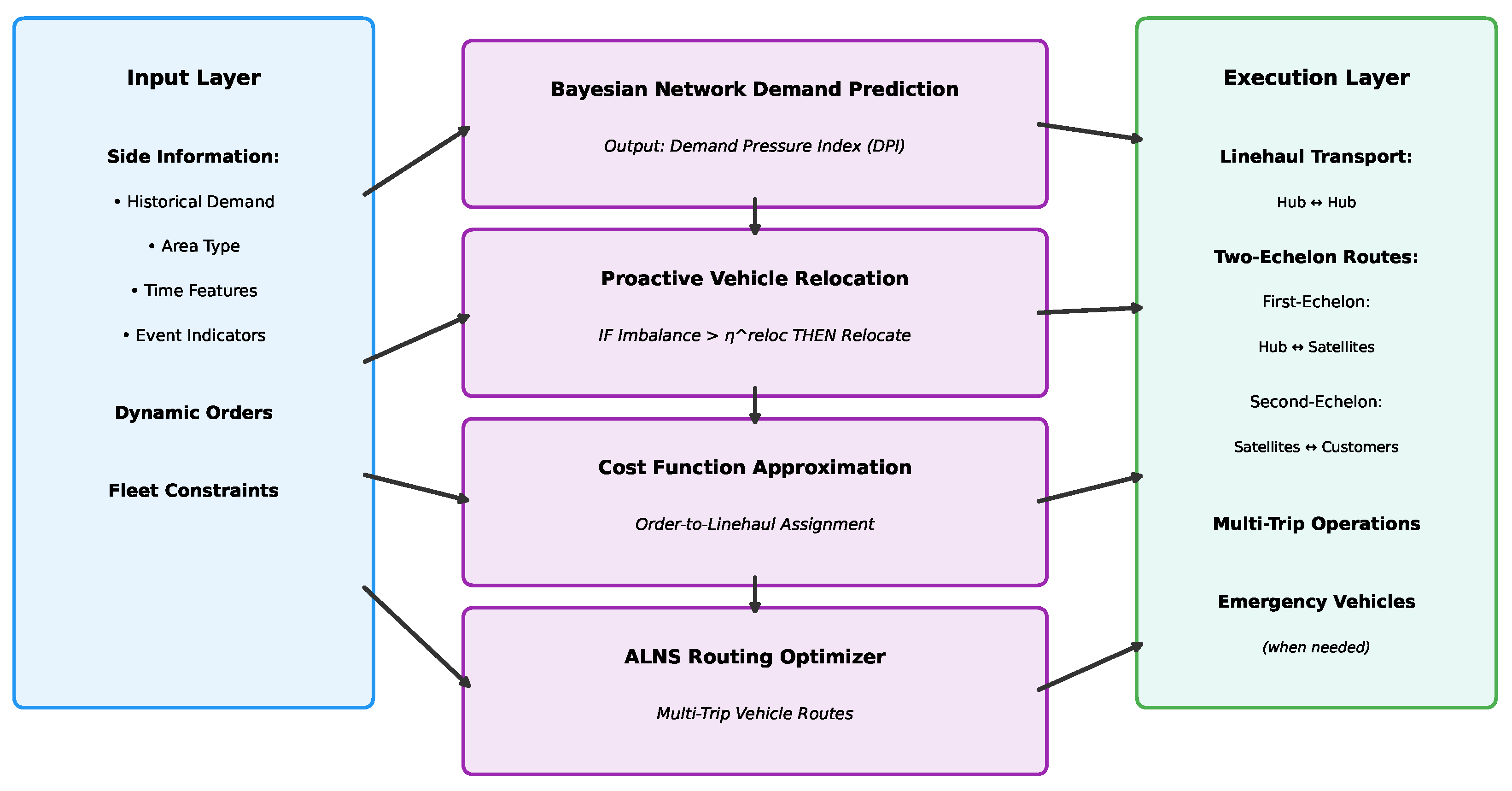
Figure 1. System architecture of the fleet-constrained metropolitan logistics problem.
Applsci 15 12609 g001
Figure 2. MDP decision process flow.
Applsci 15 12609 g002
Figure 3. Bayesian Network architecture for satellite-level demand prediction.
Applsci 15 12609 g003
Figure 4. Impact of proactive relocation on demand-supply imbalance and emergency rate reduction.
Applsci 15 12609 g004
Figure 5. Fleet size reduction achieved by multi-trip operations across different demand scenarios.
Applsci 15 12609 g005
Figure 6. Vehicle relocation frequency throughout the day. Darker colors indicate higher relocation activity. The heatmap shows average relocations per hour across 30 simulation days, demonstrating how relocation intensity varies with scenario complexity and time of day.
Applsci 15 12609 g006
Figure 7. Distribution of vehicles by number of trips performed daily.
Applsci 15 12609 g007
Figure 8. Relationship between fleet size and optimal slack weight parameter α .
Applsci 15 12609 g008
Table 1. Comparison of related literature and our study.
LiteratureProblem CharacteristicsEnvironmentOperational FeaturesAnalyticsModelSolution
Method
2EMTFCE2EDESERTMABNPDPA
Multi-Trip Vehicle Routing
Hernandez et al. [5] MIPB&P
Zhen et al. [6] MIPPSO/GA
Fermín Cueto et al. [7] MIPRobust
Pan et al. [10] MIPALNS
Two-Echelon Vehicle Routing
Dumez et al. [3] MIPMatheuristic
Lehmann Winkenbach [4] MIPMatheuristic
Karademir et al. [9] MIPLBBD
Grangier et al. [11] MIPALNS
Şahin Yaman [19] MIPB&P
Dynamic and Stochastic Dispatching
Ghilas et al. [22] SPSAA
Klapp et al. [23] MIPHeuristic
Van Heeswijk et al. [24] MDPADP
Zamal et al. [27] MDPCFA+ALNS
Sluijk et al. [28] CC-SPCG
Bayesian Networks
Garvey et al. [31] BNSimulation
Hosseini et al. [32] DBN-DTMCAnalytical
Liu et al. [33] R-DBNSA
Liu et al. [34] R-DBNSP
Hosseini Ivanov [35] ML-BNSimulation
Liu et al. [36] SV-DBNDC
Attar et al. [37] BNLearning
Harikrishnakumar Nannapaneni [38] QBNQuantum
Liu et al. [39] RA-DBNQCQP
Our workMDP+BNCFA+ALNS
Legend: 2E: Two-Echelon; MT: Multi-Trip; FC: Fleet Constraints; E2E: End-to-End Integration; DE: Dynamic Environment; SE: Stochastic Environment; RT: Real-Time Decision; MA: Metropolitan Area Focus; BN: Bayesian Network; PD: Predictive Demand; PA: Proactive Actions; MIP: Mixed Integer Programming; MDP: Markov Decision Process; SP: Stochastic Programming; CC-SP: Chance-Constrained Stochastic Programming; B&P: Branch-and-Price; ALNS: Adaptive Large Neighborhood Search; CFA: Cost Function Approximation; ADP: Approximate Dynamic Programming; LBBD: Logic-Based Benders Decomposition; SAA: Sample Average Approximation; CG: Column Generation; DBN: Dynamic Bayesian Network; R-DBN: Robust DBN; ML-BN: Multi-Layer BN; QBN: Quantum BN; RA-DBN: Risk-Averse DBN; SV-DBN: Structure-Variable DBN; DTMC: Discrete-Time Markov Chain; SA: Simulated Annealing; QCQP: Quadratically Constrained Quadratic Programming; DC: Decomposition-and-Clustering.
Table 2. System configuration parameters.
Parameter CategoryConfiguration
Geographic Layout
City structure1 hub + 2 satellites per city
Coordinate system [ 0 , 100 ] × [ 0 , 100 ] UTM grid
Hub locationCity center ( 50 , 50 )
Satellite distance from hub20–30 units
Temporal Parameters
Planning horizon (T)600 min (10 h)
Decision epoch interval ( δ )60 min
Number of epochs (K)10
Order arrival window [ 0 , 600 ] min (uniform)
Order Characteristics
Daily order volume per city150–200 orders
Order weight1–4 units (uniform random integer)
Same-day pickup window [ t arrival , t arrival + 180 ] min
Same-day delivery window [ t arrival + 120 , t arrival + 300 ] min
Next-day pickup window [ t arrival , 420 ] min
Next-day delivery window [ 540 , 600 ] min
Vehicle Specifications
First-echelon capacity ( Q 1 )75 units
First-echelon fleet sizeUnlimited
Second-echelon capacity ( Q 2 )10 units
Second-echelon fleet sizeTo be optimized
Reload time ( ρ )15 min
Service time ( φ )5 min
Maximum trip duration180 min
Cost Parameters
Fixed cost ( c fixed )150 per vehicle per day
Variable cost ( c var )2 per km
Emergency fixed cost ( c em , fixed )500 per deployment
Emergency variable cost ( c em , var )5 per km
Linehaul Configuration
   Peak hours (0–120, 480–600 min)
   Capacity72 units (80% of baseline)
   Travel time108–130 min (120% of baseline)
   Fixed/variable cost90–108/12–14.4 (120% of baseline)
   Off-peak hours (240–360 min)
   Capacity108 units (120% of baseline)
   Travel time72–86 min (80% of baseline)
   Fixed/variable cost60–72/8–9.6 (80% of baseline)
   Regular hours (120–240, 360–480 min)
   Capacity90 units (baseline)
   Travel time90–108 min (baseline)
   Fixed/variable cost75–90/10–12 (baseline)
Table 3. Overall performance comparison across three approaches.
HubsScenarioOF-STOF-MTOF-MT-R
FleetCostER (%)FleetCostER (%)FleetCostER (%)Reloc/DayImb
2MND45185,3243.236156,8754.136149,2313.23.20.28
BAL52198,6575.841158,9266.541148,7895.15.80.35
MSD58216,4827.544167,7748.244154,0726.88.40.42
3MND68278,5433.554231,1924.354219,6323.44.50.30
BAL78298,3166.260232,6877.060216,3985.57.20.38
MSD85319,6248.064243,3748.864223,0837.110.30.45
Average64.3249,4915.749.8198,4716.549.8185,2015.26.60.36
vs. OF-ST---−22.6%−20.5%+14.0%−22.6%−25.8%−8.8%--
vs. OF-MT------0%−6.7%−20.0%--
Note: Fleet represents total second-echelon vehicles across all cities. ER denotes Emergency Rate (percentage of orders requiring emergency vehicles). Cost values are daily averages over a 30-day simulation. Imb represents the average standard deviation of B γ k across satellites. Reloc/Day is the average number of vehicle relocations per day.
Table 4. Cost component analysis across all scenarios and approaches.
ScenarioComponentOF-STOF-MTOF-MT-R
FleetRoutingEmergLHFleetRoutingEmergLHFleetRoutingEmergLH+Reloc
2H-MNDAmount6750141,854672035005400118,564861034265400115,87958564096
% of Total3.676.63.61.93.475.65.52.23.677.63.92.7
2H-BALAmount7800142,56712,18035106150113,72613,65034746150110,54298284269
% of Total3.971.86.11.83.971.68.62.24.174.36.62.9
2H-MSDAmount8700146,03215,75035186600112,55417,22034006600108,12612,5464800
% of Total4.067.57.31.63.967.110.32.04.370.28.13.1
3H-MNDAmount10,200217,31811,02554578100182,56713,54553808100177,86592076460
% of Total3.778.04.02.03.579.05.92.33.781.04.22.9
3H-BALAmount11,700217,36619,53054209000178,33222,05053059000172,14615,8766376
% of Total3.972.96.51.83.976.79.52.34.279.57.32.9
3H-MSDAmount12,750219,77425,20054009600171,27427,72053469600164,53219,4047547
% of Total4.068.87.91.73.970.411.42.24.373.78.73.4
Note: Fleet represents fixed vehicle costs; Routing includes first- and second-echelon variable costs; Emerg denotes emergency vehicle costs; LH is linehaul transportation cost; LH+Reloc combines linehaul and proactive relocation costs. Percentages show each component’s share of total cost.
Table 5. Detailed relocation impact analysis.
HubsScenarioMetricTime PeriodDaily Avg
MorningAfternoonEvening
(0–200)(200–400)(400–600)
2MNDRelocations0.81.21.23.2
BN Accuracy (%)72.578.375.675.5
Cost Savings1823245623656644
BALRelocations1.52.32.05.8
BN Accuracy (%)76.282.179.479.2
Cost Savings29874123302710,137
MSDRelocations2.53.42.58.4
BN Accuracy (%)81.385.782.983.3
Cost Savings42345867360113,702
3MNDRelocations1.01.81.74.5
BN Accuracy (%)74.279.577.176.9
Cost Savings24563897320711,560
BALRelocations1.83.02.47.2
BN Accuracy (%)77.883.480.980.7
Cost Savings39875431387116,289
MSDRelocations3.24.32.810.3
BN Accuracy (%)82.787.184.284.7
Cost Savings56757234438220,291
Table 6. Optimized operational parameters across three approaches.
MethodHubsScenarioCore ParametersRelocation
α β ε η reloc ξ
OF-ST2MND0.2591582.2
BAL0.4061202.0
MSD0.551991.8
3MND0.2011622.3
BAL0.3501312.1
MSD0.5071061.9
OF-MT2MND0.4541351.8
BAL0.6071181.9
MSD0.754892.0
3MND0.4071481.7
BAL0.5551231.8
MSD0.702971.9
OF-MT-R2MND0.4541351.83.20.8
BAL0.6071181.92.51.0
MSD0.754892.02.01.2
3MND0.4071481.73.50.7
BAL0.5551231.82.80.9
MSD0.702971.92.21.1
Table 7. Real-world dataset performance comparison.
HubsScenarioLDS (Current)OF-STOF-MTOF-MT-R (Ours)
FleetCostER (%)FleetCostER (%)FleetCostER (%)FleetCostER (%)
2MND180856,20012.5135599,3408.2108489,4689.5108456,3277.2
BAL195918,54015.8150642,97810.1120514,38211.8120472,2308.9
MSD215987,45018.5165691,21511.8130529,30013.2130476,37010.3
3MND2601,286,40013.2195900,4808.7155738,39310.1155687,2467.8
BAL2851,377,90016.5220964,53010.8175750,82312.3175683,2499.5
MSD3101,475,64019.22401,032,94812.5190784,67413.8190702,29410.8
Average Improvement over LDS:
OF-ST: −23.5% fleet, −30.0% cost, −35.2% emergency rate
OF-MT: −39.1% fleet, −43.8% cost, −24.5% emergency rate
OF-MT-R: −39.1% fleet, −49.5% cost, −42.8% emergency rate
Disclaimer/Publisher’s Note: The statements, opinions and data contained in all publications are solely those of the individual author(s) and contributor(s) and not of MDPI and/or the editor(s). MDPI and/or the editor(s) disclaim responsibility for any injury to people or property resulting from any ideas, methods, instructions or products referred to in the content.