A Digital Twin of River Experiment Infrastructure Based on a 3D Game Engine and Validation of Water Flow with a Real-Scale Experiment

Abstract

Reproducing the fluid dynamics of rivers is a challenging task that involves considering various factors such as water level and flow velocity. Although numerical modeling research has been performed in this field, the intricacy of establishing these models can vary considerably based on the numerical techniques applied. Hence, this study aims to validate the effectiveness of fluid flow reproduction technology based on game engines, highlighting its real-time performance. In particular, a prototype of the digital twin (DT) of the River Experiment Center, a full-scale hydraulic experimental facility, was constructed using the Unreal Engine 5 game engine, emphasizing visibility and real-time reproduction. Fluid Flux, based on shallow-water equations and 2D height fields, was utilized to reproduce flow results, and a comparative validation was conducted using the experimental data obtained from full-scale empirical tests. The findings validated the practicality of replicating real flow patterns, even with a simplified fluid simulation aimed at reproducibility and real-time efficiency. However, specific factors must be considered for public usage such as managing rivers and urban floods. The results indicate that graphics-based flow reproduction technology can more easily integrate with other fields. Moreover, the ability to reproduce events in real time and employ visual effects is essential for efficient disaster response.

1. Introduction

A digital twin (DT) is a virtual representation of a physical system that supports decision-making through system analysis and simulation, including real-time data processing. Recently, real-world systems are increasingly being replicated in virtual environments across various fields [1,2]. The analysis and implementation of DT applications were relatively limited owing to technical limitations. However, recent technological advancements have made it possible to develop DT models that can accurately replicate various real-world systems [3]. Currently, DTs can provide indirect access to remote sites that are challenging to reach due to spatial constraints and support various interpretations and predictions of extreme flood and climate change scenarios [4,5]. In particular, DTs developed based on computational fluid dynamics (CFD) for analyzing fluid flow are being applied in various fields, such as assessing the potential for natural ventilation in cities, evaluating airflow patterns for ventilation pathway planning, and analyzing opportunities for natural ventilation in urban areas [6,7]. In river environments, which are interconnected systems influenced by natural processes and human activities, complex phenomena such as extreme floods, droughts, and pollutant dispersion occur due to climate change. Understanding and managing these complexities is essential for sustainable development and improving the quality of life [8,9]. Consequently, researchers are attempting to reproduce the complexity of river environments in virtual spaces [10]. However, virtually reproducing the constantly varying fluid dynamics of rivers is a complex process that requires the consideration of numerous constraints, including the water level, flow velocity, structures, and ecological habitats. While previous numerical modeling studies have been conducted with this objective, the complexity of constructing such models varies significantly based on the numerical methods used.

In DTs, flow representation encompasses various aspects of fluid dynamics and environmental parameters in a comprehensive and intuitive manner. Therefore, effective visualization is crucial for conveying the CFD results to city planners, policymakers, the general public, and other stakeholders [2]. Specialized fluid simulation technologies have been developed for approximately 30 years in the field of computer graphics for real-time reproduction and visualization [11]. Reeves [12] introduced particle systems to model a class of fuzzy objects. Subsequently, both grid-based and particle-based approaches have been used in computer graphics for fluid simulation. Muller (2003) [11] applied Smoothed Particle Hydrodynamics (SPH) to represent realistic fluid motion, where pressure forces are computed by interpolating local density between particles using smoothing kernel functions.

Stam [13] proposed a technique that integrates grid-based shallow-water equations (SWE) with 2D height fields to achieve efficient and stable fluid simulation. This method, which uses height map-based fluid simulation to describe the evolution of a 2D velocity field, has become increasingly significant in computer graphics technology in the 2000s [14]. Later, Hagen et al. [15] introduced the finite volume method, enabling SWE to be solved on GPUs to simulate water flow over irregular terrain. Subsequently, triangular mesh patches were created and refined to represent breaking waves, with surface tension added to SWE to simulate water flow over arbitrary surfaces [16,17]. The divergence terms were ignored, synchronous grids were used, and flow functions were employed for modeling larger bodies, such as rivers, loosely coupled with a 2D Navier–Stokes equation and pipe models, to simplify the analysis [18,19].

Unlike fluid analysis in engineering fields that requires precise analytical values, computer graphics prioritize real-time reproduction and visibility, often sacrificing some physical accuracy. Therefore, this study aims to validate the potential of game engine-based fluid flow reproduction technology, emphasizing real-time performance. To this end, a prototype of the DT of the River Experiment Center (DT of REC), a full-scale hydraulic experimental facility, was constructed using the Unreal Engine 5 (UE5) game engine, which emphasizes visibility and real-time reproduction. Fluid Flux, based on SWE and 2D height fields, was utilized to reproduce the flow results, and a comparative validation was conducted using experimental data from full-scale empirical tests. Unlike typical gaming applications, the accuracy of flow implementation must be verified when a project is intended for public purposes and practical applications.

2. Materials and Methods

2.1. Overview of Fluid Simulation

Typically, two approaches are used to analyze the fluid flow: the Lagrangian approach, which examines particle motion, and the Eulerian approach, which focuses on fluid flow at fixed points. The Navier–Stokes equations, a set of partial differential equations, are typically used as governing equations to describe fluid evolution over time. The following governing equation is used for analyzing incompressible fluids such as water (Equation (1)):

$${\displaystyle \frac{\partial \overrightarrow{\mathit{v}}}{\partial t}}=-\left(\overrightarrow{\mathit{v}}·\nabla \right)\overrightarrow{\mathit{v}}-{\displaystyle \frac{1}{\rho }}\nabla \mathrm{p}+\mathsf{\upsilon }{\nabla }^2\overrightarrow{\mathit{v}}+\overrightarrow{\mathit{f}},$$

(1)

where $\rho$ denotes the fluid density, $\overrightarrow{v}$ denotes the velocity field vector, $\mathrm{p}$ denotes the fluid pressure, $\mathsf{\upsilon }$ denotes the viscosity, $\nabla$ denotes the gradient operator, and $\overrightarrow{\mathit{f}}$ denotes external forces. The Eulerian approach analyzes the Navier–Stokes equations by dividing the flow domain into a mesh or grid. Based on the spatial discretization method, it can be classified as the finite difference method (FDM), finite volume method (FVM), or finite element method (FEM). FDM and FVM have been primarily used for fluid numerical calculations [20]. In particle motion analysis, each particle has physical properties such as velocity, pressure, and temperature, thereby eliminating the need for preprocessing tasks such as mesh generation. However, to obtain stable physical results that capture the vivid real-time reproduction of simulations, several particles are required due to the influence of kernel functions that affect particles based on their distances [11]. Essentially, when simulating a phenomenon, a trade-off exists between accuracy and real-time performance. In particular, although engineering fields require precise analytical values, media, and game production prioritize visibility and real-time reproduction, typically compromising on the physical accuracy. In grid-based fluid analysis used in graphics, which emphasizes real-time reproduction, the following distinctions are observed [13,21]: (1) the numerical significance of object surfaces interacting with fluids is reduced, enabling the usage of square grids aligned with GPU memory structures; (2) the Navier–Stokes equation is decomposed and accumulated into external force, advection, viscosity, and pressure terms for calculation; (3) the advection term, which transfers velocity across the grid, uses a semi-Lagrangian approach, which is more stable in preserving physical quantities. In the particle-based approach, we used a hybrid method combining particles and grids owing to the drawback of requiring a significant number of particles, focusing on real-time reproduction rather than solution accuracy. The SPH method is a representative example [22].

This study utilized Fluid Flux (Version 2.0), a tool within UE5 (Version 5.1.1), one of the most prominent game engines, which can implement a 2D shallow water fluid simulation-based water system. Fluid Flux simulation is based on SWE, which simplifies the full Navier–Stokes equations to represent the liquid surface as a 2D height field [21,23]. As gravity acts along the y-axis, the vertical coordinate of the water surface, the fluid simulation is represented on the x-z 2D plane, and SWE is expressed as follows to represent the conservation of mass and momentum [21,23]. Equations (2) and (3) represent a simplified form of the shallow water equations (SWE) in non-conservative form, where the material derivative is used to describe the local changes in the flow depth and velocity over time. These forms are particularly suited for real-time simulation, where numerical stability is prioritized over strict conservation:

$${\displaystyle \frac{Dh}{Dt}}=-h\nabla ·\mathit{v},$$

(2)

$${\displaystyle \frac{D\mathit{v}}{Dt}}=-g\nabla \mathsf{\eta }+a^{ext},$$

(3)

where h denotes the water depth, $\mathsf{\eta }$ denotes the water surface coordinate (terrain on the bottom+h), $v$ denotes the horizontal velocity on the x and z axes, $v=(u,w)$ denotes the horizontal velocity vector on the x and z axes, and $a^{ext}$ denotes the external acceleration. In this method, the force driving fluid movement is based on the difference in groundwater level between the adjacent cells, generating a velocity map corresponding to the rate of height change and considering the water surface as a 2D grid. Subsequently, elements that cannot be represented by the height field, such as high-speed flows, breaking waves, waterfalls, and interactions with rigid and soft objects, are converted into spray, mist, and foam particles. Here, particles are considered as simple, non-interacting point masses that exchange mass and momentum with the height field fluid, thereby reducing the computational load required in grid-based methods and enabling real-time reproduction [11,24]. Fluid Flux uses a raster-based approach where surface elevation and flow velocity are updated per grid cell using local height differences. The solver updates the velocity field frame-by-frame without solving for pressure, thus avoiding the computational burden of implicit solvers. This approach favors stability and responsiveness over exact conservation, which is acceptable in visualization-driven applications. Unlike traditional CFD solvers that use finite-volume or finite-element methods with double-precision arithmetic, Fluid Flux applies a frame-based semi-implicit update scheme using float or half-float precision to prioritize responsiveness and real-time rendering. Pressure is not directly solved; instead, flow is driven by differences in the adjacent height values.

The simulation operates in the following sequence:

-

Terrain Input: A DSM from drone photogrammetry is rasterized and loaded into UE5 as a landscape height map.

-

Initialization: Water level and boundary conditions (inflow/outflow) are assigned.

-

Numerical Update: At each frame, water depth and velocity fields are updated based on Equations (2) and (3).

-

Visual Output: The flow is rendered using materials that convert velocity and height to visual effects (e.g., foam, mist, ripples).

2.2. Introduction of the River Experiment Center and Full-Scale Experiment Validation of Flow Reproduction

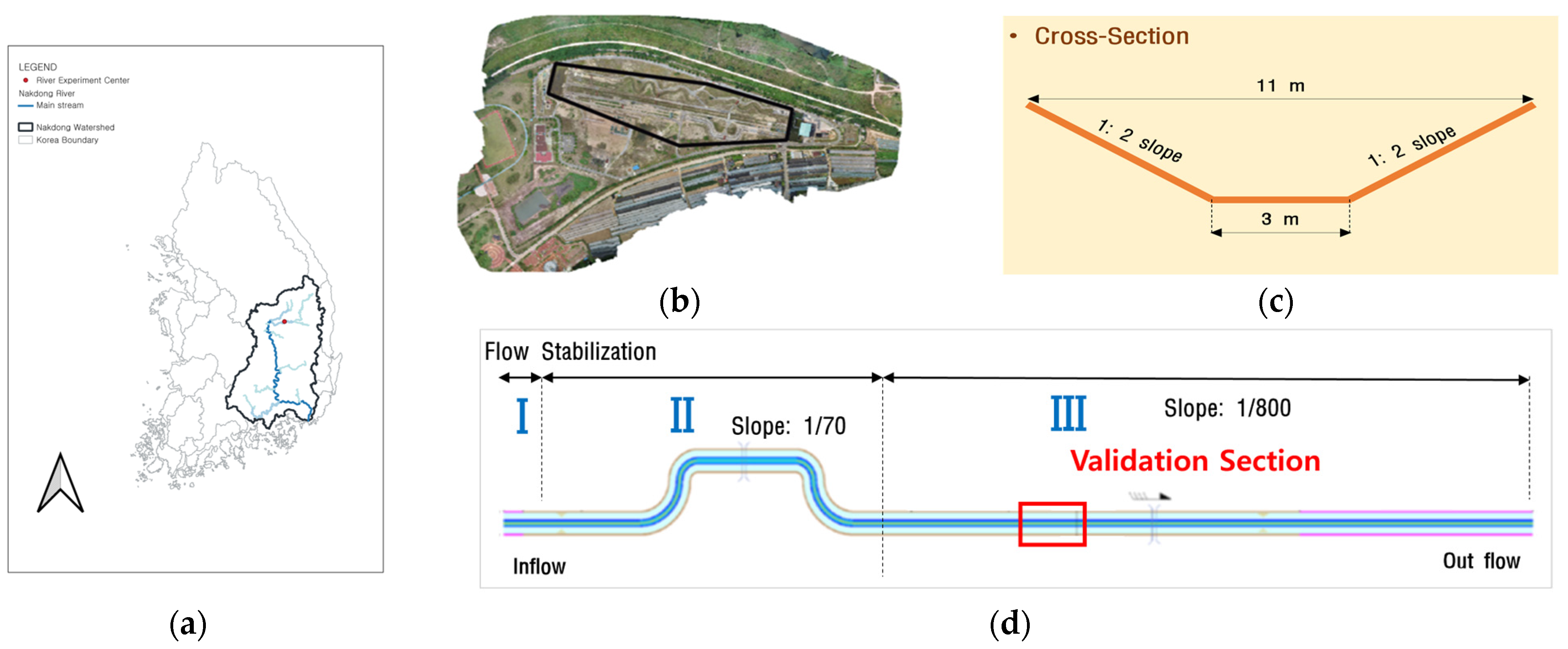
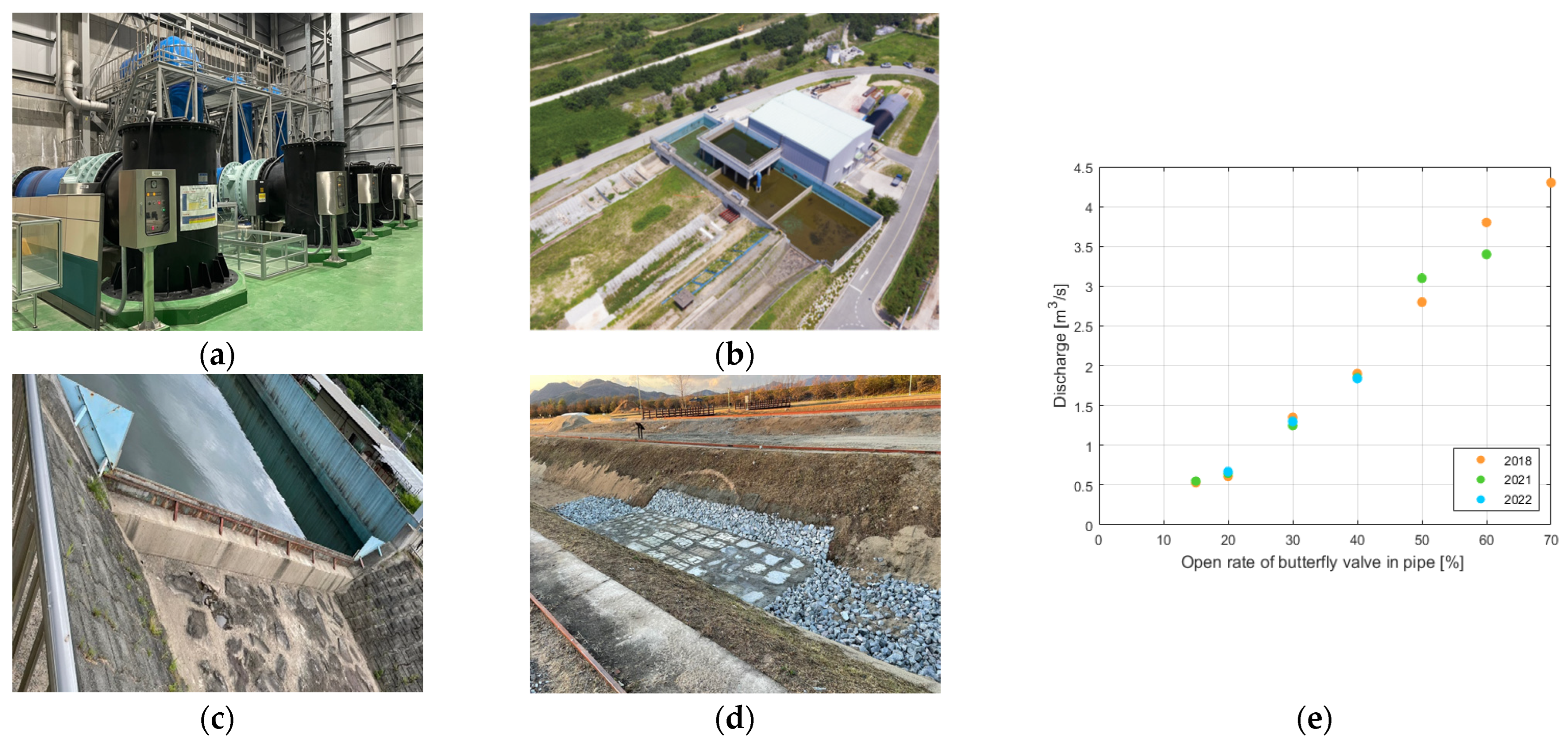
In this study, we selected the River Experiment Center of the Korea Institute of Civil Engineering and Building Technology, located in Andong, Gyeongbuk, Republic of Korea, as the research site for full-scale hydraulic experiments (Figure 1a,b). This facility comprises three channels, each approximately 600 m long, designed to stimulate small to medium-sized rivers. The flow reproduction validation in this study was conducted in channel A1, which comprises the specifications depicted in Figure 1c,d.

The River Experiment Center is located near the main Nakdong River. Water from Nakdong River is directly drawn into the facility, where up to 10 m³/s of water can be supplied to each channel through four pumps. In channel A1, where the flow validation experiment was conducted, a knife weir was used to ensure a stable water supply to the channel. Water was pumped into a high reservoir, and the flow rate was controlled through pipes connected to the main reservoir (see Figure 2a–c). This study verified the practical applicability of a DT by comparing the reproduced water flow under various flow conditions in the DT-generated terrain with the actual measurement results. In the full-scale experiment, the flow rates were categorized into three conditions (valve opening rates of 30%, 40%, and 60%) by adjusting the butterfly valve opening rate of the pipe connecting the high reservoir and the main reservoir (Figure 2b). Additionally, part of the movable sandy section of the channel was constructed as a fixed bed and designated as a standard cross-section for measurement to ensure reliable measurement results (Figure 2d; validation section in Figure 1d).

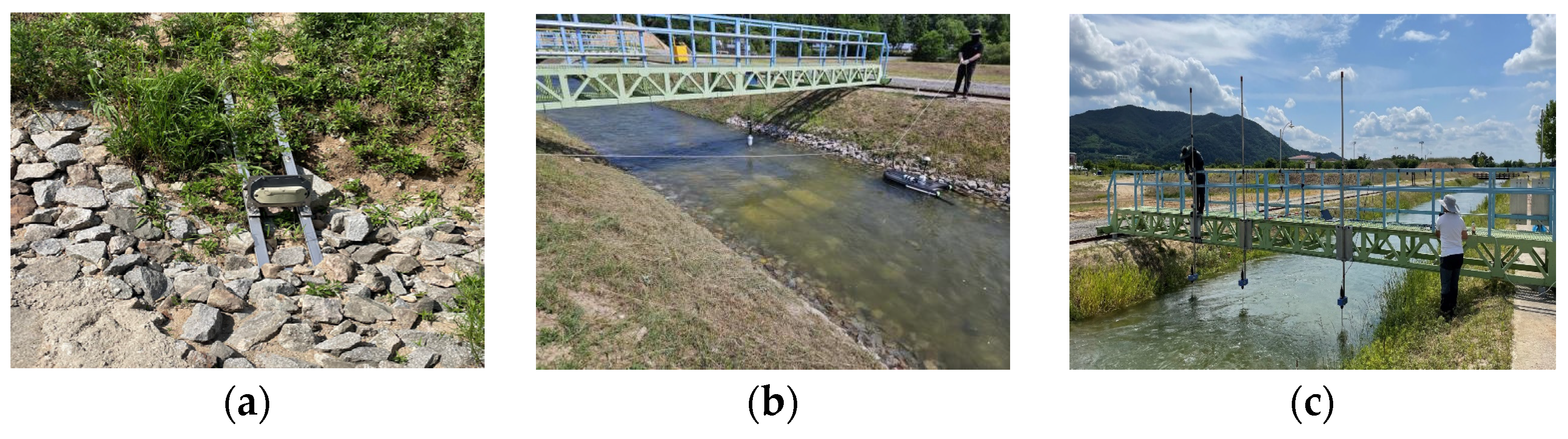
The validation experiments were continuously conducted in channel A1 of the River Experiment Center to verify the flow rates based on the butterfly valve opening rate. An increase in the opening rate presents a greater increase in the flow rate due to the nature of the butterfly valve. Figure 2e includes data from different years (2018, 2021, and 2022), demonstrating that this valve opening–discharge relationship has remained consistent across multiple calibration experiments conducted under similar conditions. For flow characteristic measurements, we utilized several methods to assess the depth, velocity, and flow rate. We employed Acoustic Doppler velocimetry (ADV) for 3D point-based velocity measurements using ultrasonic Doppler technology. For flow rate measurement, we used the acoustic Doppler current profiler (ADCP), which operates based on the Doppler effect. Additionally, we employed the workhorse horizontal ADCP (H-ADCP) model SL-3000 by SonTek (San Diego, CA, USA). This model provides index velocity derived from lateral velocity distributions and calculates the flow rate based on the input terrain and depth data. Using an ADCP (River Surveyor M9) for the validated cross-section, the measurements were repeated 19 to 31 times per condition. As ADCP cannot measure velocity in the upper and lower sections, the unmeasured sections were interpolated using a 1/6 power function based on the measured data. Additionally, we used DischargeKeeper by Seba (Kaufbeuren, Germany), which enables flow rate calculation by measuring the surface velocity and water level based on images. This device uses the surface structure image velocimetry (SSIV) technique, which estimates the velocity from the observable surface features such as ripples and waves, and obtains the vertical velocity profile using a roughness-dependent mixing length model, from which the flow rate is calculated [25,26]. Furthermore, the ground control points (GCPs) within the camera field were utilized for camera calibration, local filtering, and error velocity vector correction. The water level data were enhanced by inputting data from external analog and digital water level sensors, resulting in more accurate water level measurements.

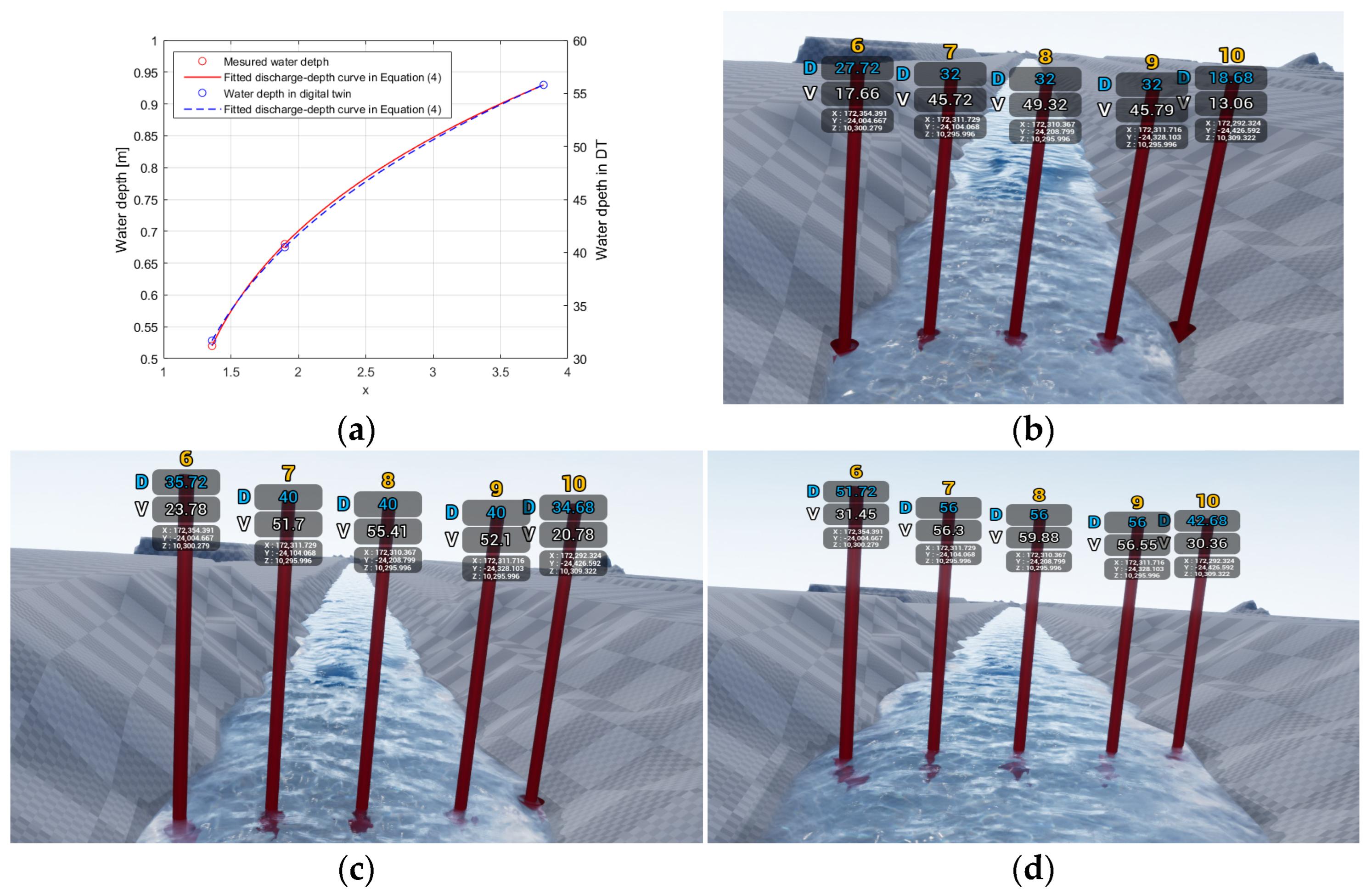
As explained in the next section, it is challenging to precisely distinguish between the three flow rate conditions in the full-scale experiment owing to the different representation methods for velocity and water depth in game engine reproductions. Consequently, we first established a water level-flow rate curve using a common water level-flow rate formula based on the actual flow rates for valve opening rates of 30%, 40%, and 60% and the measured depths at the standard cross-section (Figure 2d).

$$Q=a\times h^C$$

(4)

Here, Q denotes the flow rate, h denotes the water depth, and a and b denote the proportional and exponential constants, respectively. Subsequently, a flow rate-water level curve was generated for the reproduced water depth in the DT using the same formula, which concurs with the previously established curve to present the relationship between the reproduced and measured water depths. Lastly, we compared the velocity based on the relationship between the reproduced and measured water depths in the DT of REC.

3. Results

3.1. Precision Data Construction for the River Experiment Center and Terrain Reproduction Within the Digital Twin

As the simulated flow is reproduced based on UE5′s terrain system, accurately constructing the actual terrain is crucial. In UE, the terrain can be created using the landscape system, and digital elevation models (DEMs), which are typically used as terrain data in the raster format, can be converted to G-16 heightmap format for terrain generation. Although the terrain can be generated with DEMs of resolutions below 10 m, higher-resolution DEMs are required for accurate terrain reproduction [27]. In this study, we captured a total of 3477 images over an area of approximately 0.495 km², including the vicinity of the River Experiment Center, using an Inspire 2 drone (Zenmuse X5S, SZ DJI Technology Co., Ltd., Shenzhen, China). We deployed a total of 8 GCPs to obtain DEM and orthophoto using the structure obtained using the motion (SfM) technique (

Table 1. GCPs for Structure from Motion.

Name	Accuracy	Error			Projection Error	Marked Image
	XY/Z [m]	X (m)	Y (m)	Z (m)	Y (pixel)	Z (m)
GCP 1	0.02/0.02	0.008	−0.012	−0.018	0.639	58
GCP 2	0.02/0.02	0.000	−0.024	0.075	0.644	139
GCP 3	0.02/0.02	−0.007	0.023	−0.048	0.363	77
GCP 4	0.02/0.02	0.001	−0.002	0.003	0.676	42
GCP 5	0.02/0.02	0.063	−0.03	−0.006	0.545	109
GCP 6	0.02/0.02	−0.029	0.02	0.023	0.737	120
GCP 7	0.02/0.02	−0.017	−0.003	0.003	0.392	84
GCP 8	0.02/0.02	−0.009	0.018	−0.041	0.357	41

).

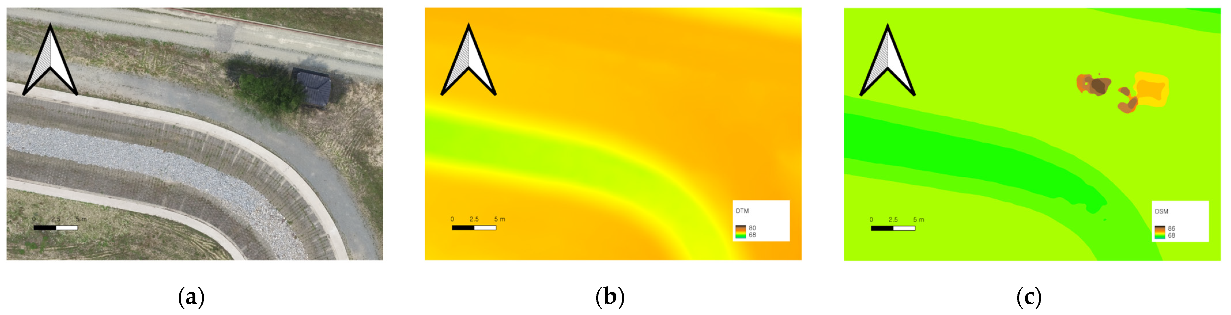
A total of 3473 images were used to generate the composite image, with an average ground sampling distance of 2.78 cm, representing the distance between the centers of two consecutive pixels. The root mean square error (RMSE) for georeferencing was 0.026 m. The digital surface model (DSM) obtained from the SfM technique using actual images is based on the heights of various structures and vegetation present on the terrain, rather than only on the terrain elevation (Figure 3).

Although various methods can be used to convert DSM to a digital terrain model (DTM), the converted DTM does not contain accurate height information [28]. In the DSM, objects such as bridges and vegetation located above the channel are recognized as part of the terrain. However, as Fluid Flux employs top-down rendering, this can vary significantly from the actual flow reproduction. Additionally, owing to the various applications of the developed DT of REC, such as simulating floods and analyzing changes in flow due to structures, it enabled users to edit the terrain directly and continuously update it with new DEMs. For the DT of the REC prototype, a high-resolution DEM was used based on the composite image results, and only the minimum area containing the three channels of the REC was reproduced for flow reproduction purposes (black polygon in Figure 1b).

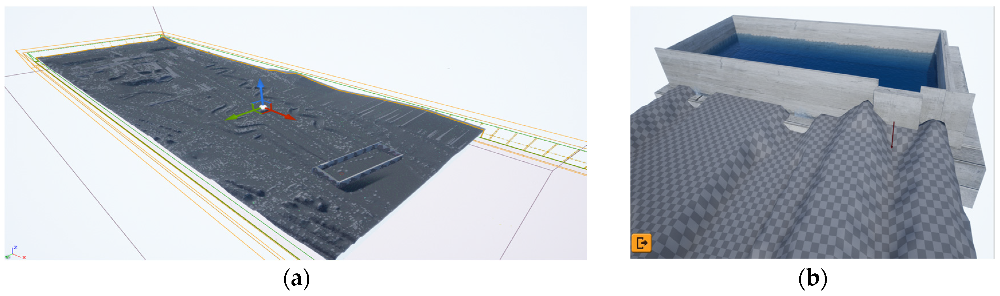
In Unreal Engine 5, the landscapes comprise multiple square components, which serve as the basic units for rendering, collision detection, and simulation interactions. Each component is generated with a defined resolution and detail level, which affects both the visual fidelity and simulation performance of the terrain. A landscape component comprises one or more sections, and each section comprises a grid of quads, with each quad defined by four corner vertices forming a square tile [27]. These tiles collectively define the surface geometry of the terrain through height values stored in a heightmap texture. In this study, the area selected for simulation spans approximately 71,004.8 m². The UE5 terrain reconstruction comprises 480 landscape components, each with 2 × 2 sections and 127 × 127 quads per component. This presents an effective terrain resolution of 8129 × 3811 pixels across the entire simulation domain (Figure 4).

This level of detail was selected to achieve a balance between the simulation accuracy and computational efficiency. A higher terrain resolution presents finer representation of the elevation gradients and hydraulic features, which is essential for accurately modeling the flow behavior over small-scale topographic variations. However, increasing the resolution also requires greater memory and processing resources, especially in real-time rendering environments like UE5. The selected resolution ensures that the key topographic features of the experimental flume are preserved while maintaining stable real-time performance.

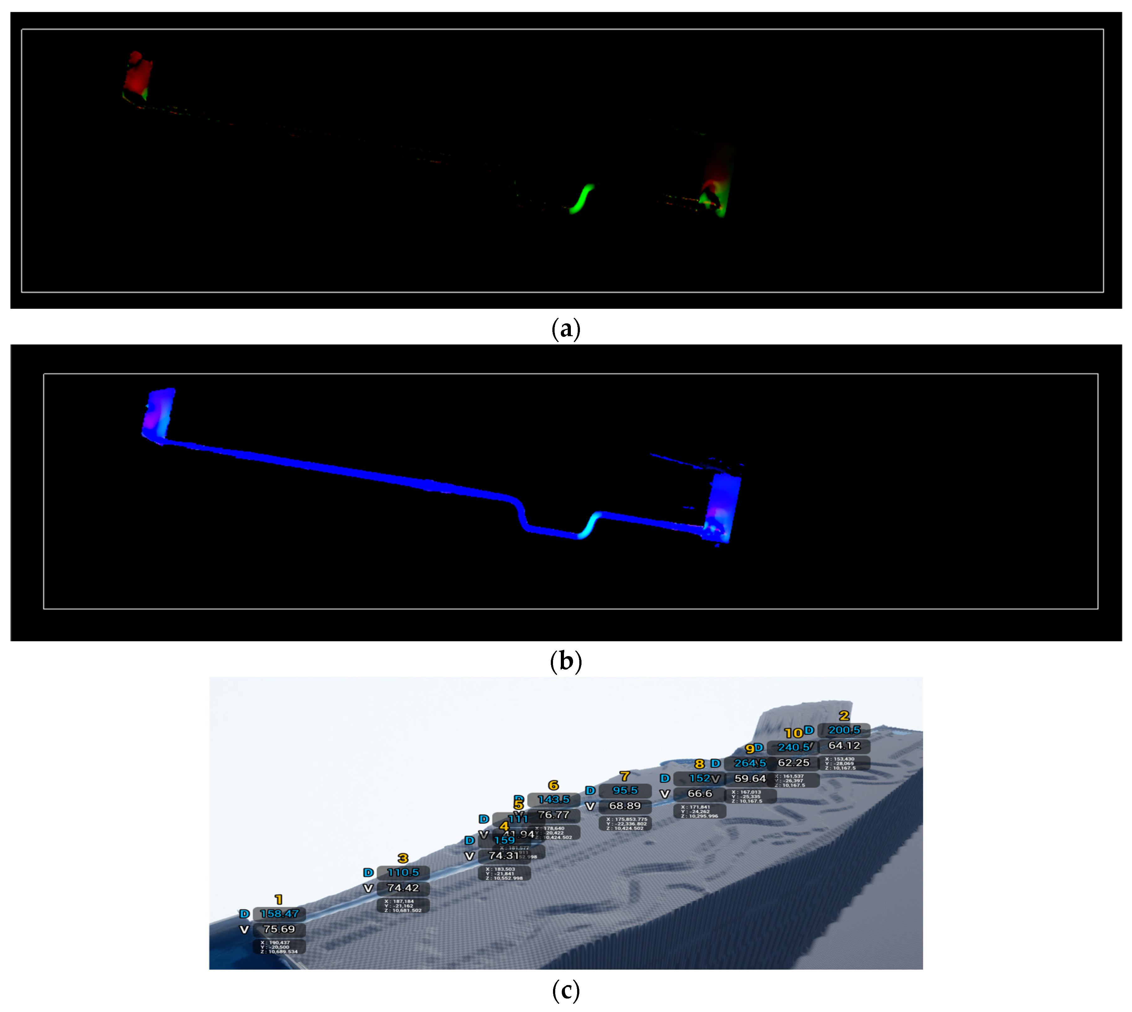
To reproduce the water flow, a reservoir was created as the point where water is generated (emitter position), and a sink point was established at the bottom of the channel for fluid removal. The DT was designed with an adjustable gate set as an open boundary as it is challenging to supply water to the reservoir using pumps owing to the pump efficiency and the overall water supply system. The water amount generated inside the reservoir could be adjusted, enabling direct control of the flow supplied to the channel (Figure 4b). We primarily aim to validate the flow reproduction results of the DT of REC using Fluid Flux by comparing them with the actual flow, using water depth and velocity as the flow characteristic factors for validation. As UE employs an internal world coordinate system, accurately reproducing the actual location information is challenging, and Fluid Flux cannot numerically represent the actual fluid velocity. Therefore, to visualize the simulated flow field, a mesh was generated using the terrain vertex data previously reconstructed from drone-based photogrammetry. This mesh was used to represent water depth and flow velocity by encoding the values into an RGB color model. Specifically, the blue (B) channel was used to indicate water depth, with darker blues corresponding to deeper water. A dedicated material layer was applied in UE5/Fluid Flux to construct this height-based depth map. To visualize horizontal velocity, the red (R) and green (G) channels were used to represent flow speed in the x (streamwise) and z (transverse) directions, respectively. In this way, directional flow components could be intuitively understood through color variation across the mesh. The resulting composite image (Figure 5) provides a pixel-wise visualization of flow characteristics directly mapped from numerical results to rendered output.

Subsequently, the red and green values (range: 0–255) for the x and z directions were adjusted to a range of 0–100 by converting to vector length values within the blueprint. The speed from the converted vector length values was represented as follows:

$$\left|V\right|=\sqrt{x^2+y^2},$$

(5)

Within the DT of the empirical experiment facility, flow reproduction enables the verification of the depth (D) and velocity (V) values at the desired locations. The UE world coordinates (x, y, z) of the locations representing the depth and velocity are also available (Figure 5c). Key simulation parameters such as the time step (1/60 s), simulation resolution (2048 × 2048), and simulation scale (1.0) were set and post-processing effects and ray tracing were disabled, while Lumen was enabled at medium quality. All simulations were performed on a high-performance workstation equipped with an Intel^® Core™ i9-9960X CPU @ 3.10 GHz, 256 GB DDR4 RAM, and an NVIDIA GeForce RTX 3090 GPU (Santa Clara, CA, USA).

3.2. Full-Scale Experiment Results and Flow Reproduction

In the full-scale experiment conducted for the comparison of flow velocities between the reproduced flow in the DT of REC and actual measured velocities, various measurement methods were employed (Figure 6).

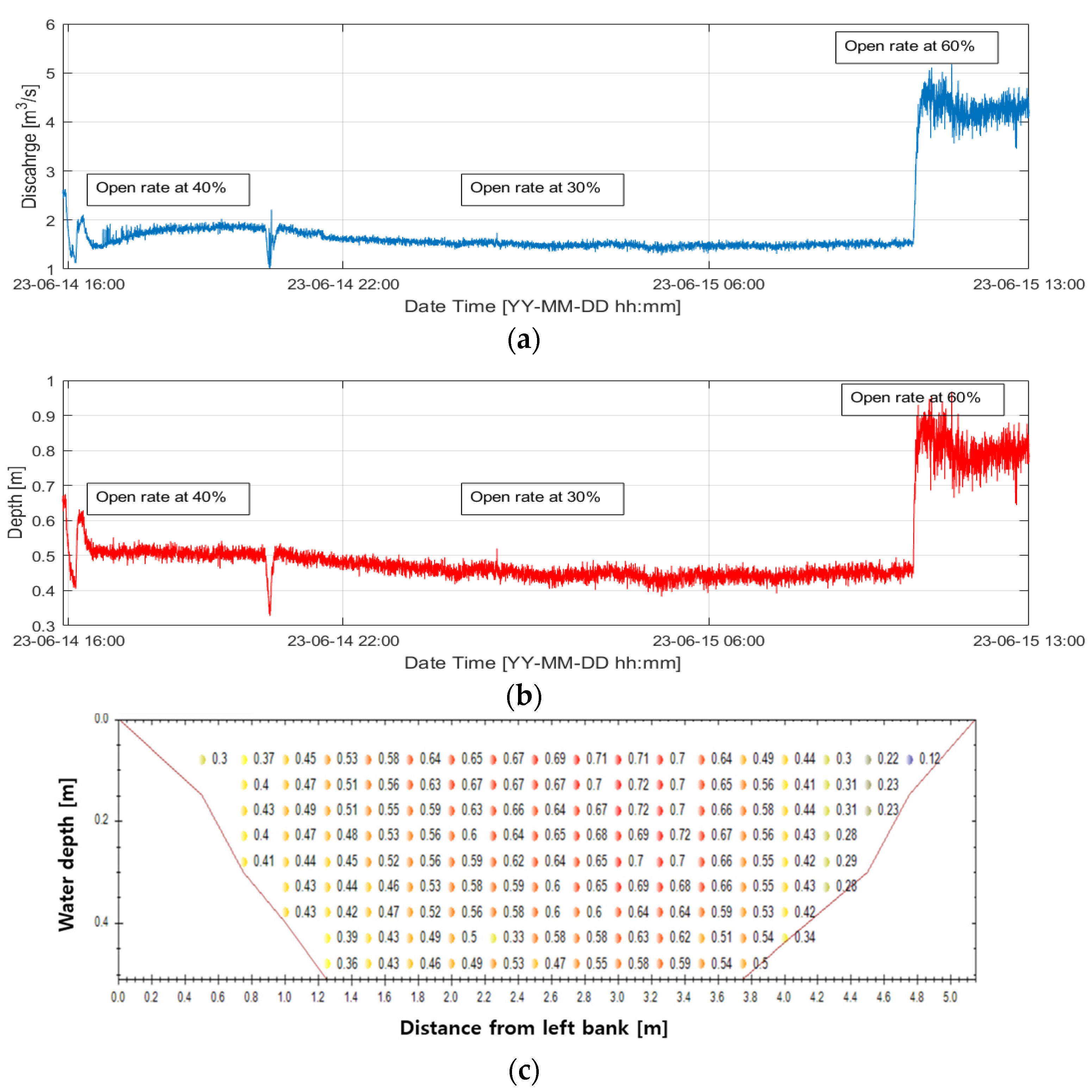
The H-ADCP (SL-3000 was installed in a fixed position; it calculates the flow rate based on the index velocity obtained from the lateral velocity distributions and pre-input terrain and depth data (Figure 6a). However, as H-ADCP does not measure the entire cross-section, it was considered to be less accurate than other devices and was used to monitor the continuous flow supply during the experiment (Figure 7a).

For the valve opening rates of 30% and 60%, we performed detailed measurements across the entire cross-section using ADV, and ADV data were averaged over 10 s at 25 Hz (~250 samples per point) to ensure stability. Additionally,

Table 2. Measured water velocity, water depth, and discharge by ADV, ADCP, and DischargeKeeper.

	Valve Opening Rate 30%			Valve Opening Rate 40%			Valve Opening Rate 60%
	Average Velocity [m/s]	Depth [m]	Flow Rate [m/s]	Average Velocity [m/s]	Depth [m]	Flow Rate [m3/s]	Average Velocity [m/s]	Depth [m]	Flow Rate [m3/s]
ADV	0.51	-	1.21	-	-	-	0.78	-	3.81
ADCP (M9)	0.53	0.51	1.35	0.63	0.68	1.98	0.79	0.92	3.82
DischargeKeeper	0.58	-	1.31	0.65	-	2.02	0.81	-	3.98

presents the results from the portable ADCP and DischargeKeeper for 30%, 40%, and 60% valve opening rates. Here, velocity represents the average cross-sectional velocity and depth represents the depth at the center of the cross-section. Although each measurement device has some margin of error, the results did not significantly vary from the previously established valve opening rate-flow rate relationship. As mentioned earlier, it is difficult to match the exact flow values for the valve opening rates of 30% and 60% of the pipe pumps supplying water from the high to the main reservoir. Therefore, the flow, measured depth, and relationship curve between flow and reproduced depth within the DT were aligned as closely as possible to reproduce the flow based on the relationship between the reproduced and measured depths (Figure 8a).

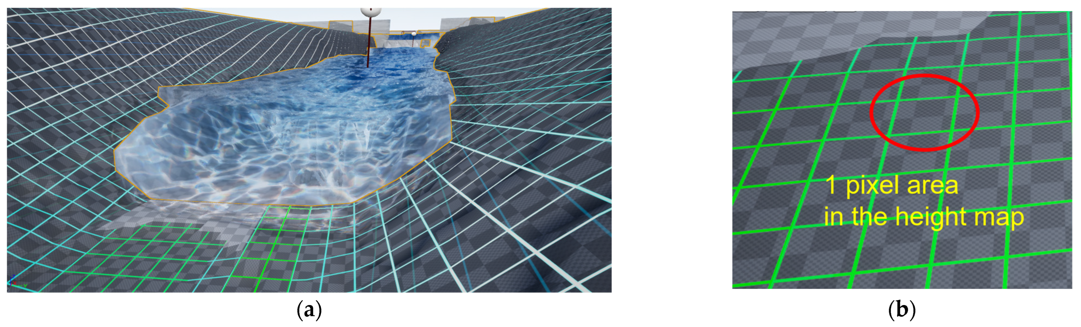
The discrepancy between the actual flow-measured depth and the reproduced depth in the DT was attributed to the depth data represented in the scaled ranges within the height map rather than at a single pixel level. Essentially, this difference was attributed to the discrepancy between the resolution of the height map where the depth data were stored, along with the actual resolution in UE.

3.3. Comparison of Full-Scale Experiment Results and Flow Reproduction Results (Velocity Distribution)

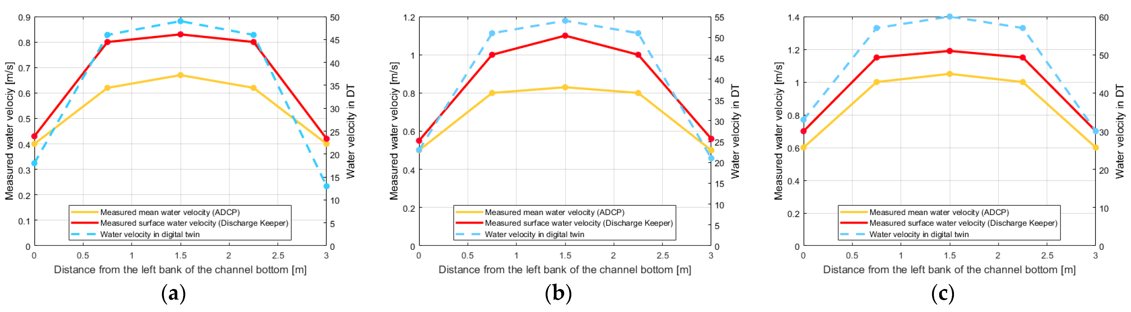
For the DT reproduction results based on depth for the valve opening rates of 30%, 40%, and 60% discussed in Section 3.2, velocity validation was performed at five locations spaced 0.75 m apart on the left bank at a 3 m distance from the channel bottom along the cross-section. In particular, the depth-averaged velocity from ADCP, surface velocity from DischargeKeeper, and velocity reproduced in the DT obtained using Equation (2) were compared at each location (Figure 9). To ensure reliable comparison, the transient phase of the simulation—characterized by initial flow instability—was excluded. Only the results from the stabilized period, after the system reached a quasi-steady state, were used for validation against experimental data.

In all the cases, the reproduced velocity in the DT increased as it approached the center of the channel. Notably, the reproduced velocity in the DT appeared to be closer to the surface velocity. This is likely because, after simulating the flow using the 2D height map and SWE, the calculated flow direction and speed were applied to particles for realistic reproduction, similar to SSIV, which also tracked the flow using the observable features such as ripples, waves, and surface patterns. Additionally, as the flow rate conditions increased, the difference between the actual measured surface velocity and reproduced velocity increased, likely because factors such as wind, which affect actual surface velocity, were not considered in the reproduced velocity.

4. Discussion

In this study, we constructed a DT of an empirical hydraulic experiment facility using terrain information implemented in Unreal Engine 5 (UE5) and Fluid Flux, which simulates flow based on a 2D height map and the SWE. The DT flow simulation was validated against full-scale experimental measurements of water velocity and depth. The results demonstrated that, even with a simplified fluid solver focused on reproducibility and real-time performance, key flow features such as lateral velocity distribution and flow-depth relationships can be replicated to a satisfactory degree. While real-time reproduction and vivid visualization are important, accurate values for water depth and velocity are also critical. However, to ensure scientific robustness and applicability to real-world river and urban flood management, several limitations and challenges must be considered. One key limitation is the use of top-down rendering in Fluid Flux, which restricts accurate representation of complex hydraulic features such as bridge piers, floodplain vegetation, and urban structures like culverts and sewer systems. This simplification may lead to loss of local flow detail that is critical for flood hazard assessment. Moreover, the simulation accuracy is constrained by the resolution of the height map and mesh. As shown in Figure 10, terrain resolution degrades at larger spatial scales. A mesh sensitivity analysis—currently absent from this work—is required to better understand the trade-off between computational cost and predictive accuracy. We identify this as an important direction for future research.

In addition, the normalized velocity range (0–100) introduces non-negligible uncertainty, especially when comparing reproduced results with physical measurements. The simulation also lacks multi-depth velocity stratification, as Fluid Flux models the flow as a surface-level phenomenon. This limits its suitability for applications requiring vertical flow structure analysis, such as sediment transport or pollutant dispersion. Nevertheless, the DT successfully captured the surface velocity trends observed in the field, particularly when compared to surface-sensitive devices like DischargeKeeper. This demonstrates that real-time, visually enhanced simulation systems can complement conventional CFD tools, particularly in contexts such as stakeholder engagement, emergency preparedness training, and rapid scenario testing. Future research will focus on extending the framework to handle unsteady flows, sediment dynamics, and inundation modeling. We also plan to integrate real-time sensor networks and forecasting systems to support responsive DT applications. Furthermore, the platform’s accessibility and visual clarity position it as a powerful educational and decision-support tool for river management and urban planning.

5. Conclusions

In this study, a prototype DT of the River Experiment Center (REC), an empirical hydraulic experiment facility, was constructed using Unreal Engine 5. The Fluid Flux tool, which simulates fluid flow based on a 2D height field and the SWE, was employed to reproduce the water flow in real time with visual clarity. The resulting simulation was validated using full-scale experimental data under three valve opening conditions (30%, 40%, 60%). The terrain model was generated using drone imagery and GCPs, reconstructed via Pix4D, and implemented in UE5 with a resolution of 8129 × 3811 over an area of approximately 71,004.8 m². To evaluate the simulated flow, flow-depth relationship curves were constructed for each experimental condition, allowing comparison with the depth values reproduced in the DT. Moreover, lateral velocity profiles across the channel were compared, and the reproduced flow captured the trend of increased surface velocity toward the channel center. Notably, the reproduced flow showed stronger agreement with surface velocity measurements from DischargeKeeper than with depth-averaged velocities from ADCP, likely due to the visual particle system in Fluid Flux resembling the surface-based detection mechanism of DischargeKeeper. The results indicate that even a simplified simulation framework based on a game engine can successfully reproduce key flow characteristics and support practical interpretation. However, the study is currently limited by the scale of experimental comparison, focusing on a single validation section. Future comparisons with high-fidelity CFD models may help quantify and reduce uncertainty, enabling more rigorous assessment. Nevertheless, this study is one of the first to validate the feasibility of real-time, graphics-based fluid flow simulation using experimental data, and demonstrates its potential for interdisciplinary applications. In particular, it highlights the utility of game engine-based DTs in providing visually intuitive, responsive, and flexible platforms for river simulation. Future research will focus on extending simulation capabilities to include unsteady flow, sediment transport, and urban flood scenarios. In addition, the integration of this DT platform with real-time sensor networks and forecasting systems will be explored. This system also has potential as an educational and stakeholder engagement tool in the context of river and floodplain management. Ultimately, the primary goal of this study is not only to demonstrate the feasibility of game engine-based flow reproduction but also to emphasize the significance of outlining its limitations, future research directions, and potential applications in practical settings such as disaster response and interdisciplinary river management.

In summary, while accuracy is fundamental in hydrodynamic modeling, real-time responsiveness and visual clarity are equally important in applications such as disaster response and stakeholder communication. With ongoing advancements in GPU/CPU performance and simulation technologies, real-time flow modeling using graphics-based tools can complement traditional CFD by enhancing accessibility, speed, and interdisciplinary integration.

References

1. Rasheed, A.; San, O.; Kvamsdal, T. Digital twin: Values, challenges and enablers from a modeling perspective. IEEE Access 2020, 8, 21980–22012. [Google Scholar] [CrossRef] [Scilit]
2. Mitkov, R.; Pantusheva, M.; Petrova-Antonova, D.; Naserentin, V.; Logg, A. The role of computational fluid dynamics within city digital twins: Opportunities and challenges. ISPRS Ann. Photogramm. Remote Sens. Spat. Inf. Sci. 2024, 10, 131–136. [Google Scholar] [CrossRef] [Scilit]
3. Ketzler, B.; Naserentin, V.; Latino, F.; Zangelidis, C.; Thuvander, L.; Logg, A. Digital twins for cities: A state of the art review. Built Environ. 2020, 46, 547–573. [Google Scholar] [CrossRef] [Scilit]
4. Henriksen, H.J.; Schneider, R.; Koch, J.; Ondracek, M.; Troldborg, L.; Seidenfaden, I.K.; Kragh, S.; Bøgh, E.; Stisen, S. A new digital twin for climate change adaptation, water management, and disaster risk reduction (HIP digital twin). Water 2022, 15, 25. [Google Scholar] [CrossRef] [Scilit]
5. Tarpanelli, A.; Bonaccorsi, B.; Sinagra, M.; Domeneghetti, A.; Brocca, L.; Barbetta, S. Flooding in the Digital Twin Earth: The case study of the Enza River levee breach in December 2017. Water 2023, 15, 1644. [Google Scholar] [CrossRef] [Scilit]
6. Chung, D.H.J.; Choo, M.-L.L. Computational fluid dynamics for urban design: The prospects for greater integration. Int. J. Archit. Comput. 2011, 9, 33–53. [Google Scholar] [CrossRef] [Scilit]
7. Tong, Z.; Luo, Y.; Zhou, J. Mapping the urban natural ventilation potential by hydrological simulation. Build. Simul. 2021, 14, 351–364. [Google Scholar] [CrossRef] [Scilit]
8. Kang, W.; Jang, E.K.; Yang, C.Y.; Julien, P.Y. Geospatial analysis and model development for specific degradation in South Korea using model tree data mining. Catena 2021, 200, 105142. [Google Scholar] [CrossRef] [Scilit]
9. Kang, W.; Lee, D.H. Experimental study of seepage in levee with transverse structure and water barrier. Geom. Nat. Hazards Risk 2024, 15, 2300811. [Google Scholar] [CrossRef] [Scilit]
10. Park, D.; You, H. A digital twin dam and watershed management platform. Water 2023, 15, 2106. [Google Scholar] [CrossRef] [Scilit]
11. Müller, M.; Charypar, D.; Gross, M. Particle-based fluid simulation for interactive applications. In Proceedings of the 2003 ACM SIGGRAPH/Eurographics Symposium on Computer Animation, San Diego, CA, USA, 26–27 July 2003; ACM Digital Library: New York, NY, USA, 2003; pp. 154–159. [Google Scholar]
12. Reeves, W.T. Particle systems—A technique for modeling a class of fuzzy objects. In Seminal Graphics: Pioneering Efforts That Shaped the Field; ACM Press: New York, NY, USA, 1998; pp. 203–220. [Google Scholar]
13. Stam, J. Real-time fluid dynamics for games. In Proceedings of the Game Developer Conference, San Jose, CA, USA, 4–8 March 2003; CRC Press: San Francisco, CA, USA, 2003; Volume 18. [Google Scholar]
14. Layton, A.T.; van de Panne, M. A numerically efficient and stable algorithm for animating water waves. Vis. Comput. 2002, 18, 41–53. [Google Scholar] [CrossRef] [Scilit]
15. Hagen, T.R.; Hjelmervik, J.M.; Lie, K.A.; Natvig, J.R.; Ofstad Henriksen, M.O. Visual simulation of shallow-water waves. Simul. Modell. Pract. Theor. 2005, 13, 716–726. [Google Scholar] [CrossRef] [Scilit]
16. Thurey, N.; Muller-Fischer, M.; Schirm, S.; Gross, M. Real-time breaking waves for shallow water simulations. In Proceedings of the Pacific Conference on Computer Graphics and Applications, Maui, HI, USA, 29 October–2 November 2007; IEEE Computer Society: Los Alamitos, CA, USA, 2007; pp. 39–46. [Google Scholar]
17. Wang, Z.L.; Geng, Y.F. Two-dimensional shallow water equations with porosity and their numerical scheme on unstructured grids. Water Sci. Eng. 2013, 6, 91–105. [Google Scholar]
18. Burrell, T.; Arnold, D.; Brooks, S. Advected river textures. Comput. Animat. Virtual Worlds 2009, 20, 163–173. [Google Scholar] [CrossRef] [Scilit]
19. Yu, Q.; Neyret, F.; Bruneton, E.; Holzschuch, N. Scalable real-time animation of rivers. Proc. Eurographics 2009, 28, 239–248. [Google Scholar] [CrossRef] [Scilit]
20. Chen, F.; Sondak, D.; Protopapas, P.; Mattheakis, M.; Liu, S.; Agarwal, D.; Di Giovanni, M. Neurodiffeq: A python package for solving differential equations with neural networks. J. Open Source Softw. 2020, 5, 1931. [Google Scholar] [CrossRef] [Scilit]
21. Chentanez, N.; Müller, M. Real-time simulation of large bodies of water with small scale details. In Symposium on Computer Animation; The Eurographics Association: Eindhoven, The Netherlands, 2010; pp. 197–206. [Google Scholar]
22. Desbrun, M.; Gascuel, M.P. Smoothed particles: A new paradigm for animating highly deformable bodies. In Computer Animation and Simulation; Springer: Vienna, Austria, 1996; pp. 61–76. [Google Scholar]
23. Chentanez, N.; Müller, M.; Kim, T.Y. Coupling 3D Eulerian, heightfield and particle methods for interactive simulation of large scale liquid phenomena. IEEE Trans. Vis. Comput. Graph. 2015, 21, 1116–1128. [Google Scholar] [CrossRef] [Scilit]
24. Hu, Y.; Fang, Y.; Ge, Z.; Qu, Z.; Zhu, Y.; Pradhana, A.; Jiang, C. A moving least squares material point method with displacement discontinuity and two-way rigid body coupling. ACM Trans. Graph. 2018, 37, 150. [Google Scholar] [CrossRef] [Scilit]
25. Absi, R. A roughness and time dependent mixing length equation. Doboku Gakkai Ronbunshuu B 2006, 62, 437–446. [Google Scholar] [CrossRef] [Scilit]
26. Muste, M.; Fujita, I.; Hauet, A. Large-scale particle image velocimetry for measurements in riverine environments. Water Resour. Res. 2008, 44. [Google Scholar] [CrossRef] [Scilit]
27. Epic Games Inc. Terrains from DEMs; 13 November 2023. Available online: https://docs.unrealengine.com/udk/Three/TerrainsFromDEMs.html (accessed on 17 November 2025).
28. Julzarika, A.; Harintaka. Free global DEM: Converting DSM to DTM and ITS applications. Int. Arch. Photogramm. Remote Sens. Spat. Inf. Sci. 2019, 42, 319–325. [Google Scholar] [CrossRef] [Scilit]
Figure 1. (a) Location of Andong River Experiment Center where the game engine-based flow reproduction validation experiment was conducted, (b) the entire section targeted for reproduction, (c) cross-sectional specifications of the experimental channel, and (d) overall specifications of the channel.
Applsci 15 12507 g001
Figure 2. Infrastructure for full-scale experiments at Andong River Experiment Center: (a) pump facility, (b) high and main reservoirs, (c) knife weir, (d) fixed bed standard cross-section, (e) Discharge by butterfly valve opening rate.
Applsci 15 12507 g002
Figure 3. Difference between DSM and DTM in the drone survey results of the River Experiment Center: (a) orthophoto; (b) DTM; (c) DSM.
Applsci 15 12507 g003
Figure 4. (a) Terrain reproduction result based on DSM, and (b) constructed reservoirs and gates for flow control.
Applsci 15 12507 g004
Figure 5. (a) R, G velocity map associated with x and z direction speeds rendered as a target, (b) B height map associated with depth using R, G values, (c) final reproduced depth (D) and velocity (V) within the DT.
Applsci 15 12507 g005
Figure 6. Devices used for velocity measurement: (a) workhorse horizontal ADCP, (b) River-Surveyor M9, and (c) acoustic Doppler velocimeter.
Applsci 15 12507 g006
Figure 7. Cross-sectional flow measurement results: (a) discharge monitoring results from H-ADCP, (b) depth monitoring results from H-ADCP, and (c) measurement results for 30% butterfly valve opening rate using ADV.
Applsci 15 12507 g007
Figure 8. Flow reproduction results within the DT of the experimental facility: (a) comparison between reproduced and measured depth, (b) reproduction result for 30% butterfly valve opening rate, (c) reproduction result for 40% butterfly valve opening rate, and (d) reproduction result for 60% butterfly valve opening rate.
Applsci 15 12507 g008
Figure 9. Comparison between reproduced velocity in DT and measured velocity: (a) 30% valve opening rate, (b) 40% valve opening rate, and (c) 60% valve opening rate.
Applsci 15 12507 g009
Figure 10. (a) A water surface created using water height texture data, and (b) an area of a single pixel projected onto the height map texture.
Applsci 15 12507 g010