Article

A Novel Hybrid Framework for Stock Price Prediction Integrating Adaptive Signal Decomposition and Multi-Scale Feature Extraction

1
Department of Information Systems, City University of Hong Kong, Tat Chee Avenue, Kowloon, Hong Kong
2
Department of Computer Science, City University of Hong Kong, Tat Chee Avenue, Kowloon, Hong Kong
3
Department of Logistics and Maritime Studies, Hong Kong Polytechnic University, Hung Hom, Kowloon, Hong Kong
4
Department of Management, City University of Hong Kong, Tat Chee Avenue, Kowloon, Hong Kong
*
Author to whom correspondence should be addressed.
Appl. Sci. 2025, 15(23), 12450; https://doi.org/10.3390/app152312450
Submission received: 18 October 2025 / Revised: 12 November 2025 / Accepted: 13 November 2025 / Published: 24 November 2025
(This article belongs to the Special Issue Advanced Methods for Time Series Forecasting)

Abstract

To address the issue of low prediction accuracy due to the inherent high noise and non-stationary characteristics of stock price series, this paper proposes a novel stock price prediction framework (CVASD-MDCM-Informer) that integrates adaptive signal decomposition with multi-scale feature extraction. The framework first employs a CVASD module, which is a variational mode decomposition (VMD) method adaptively optimized by a porcupine optimization (CPO) algorithm, to decompose the original stock price series into a series of intrinsic mode functions (IMFs) with different frequency characteristics, effectively separating noise and multi-frequency signals. Subsequently, the decomposed components are input into a prediction network based on Informer. In the feature extraction phase, this paper designs a multi-scale dilated convolution module (MDCM) to replace the standard convolution of the Informer, enhancing the model’s ability to capture short-term fluctuations and long-term trends by using convolution kernels with different dilation rates in parallel. Finally, the prediction results of each component are integrated to obtain the final predicted value. Experimental results on three representative industry datasets (Information Technology, Finance, and Consumer Staples) of the US S&P 500 index show that, compared to several advanced baseline models, the proposed framework demonstrates significant advantages in multiple evaluation metrics such as MAE, MSE, and RMSE. Ablation experiments further validate the effectiveness of the two core modules, CVASD and MDCM. The study indicates that the framework can effectively handle complex financial time series, providing a new solution for stock price prediction.

1. Introduction

Stock market data is characterized by high noise, non-stationarity, and non-linearity, which makes predicting future trends from historical prices a significant yet challenging task in financial research [1]. The prediction of stock prices is directly related to risk mitigation, asset allocation, and investment decisions, serving as a critical basis for market analysis by investors and regulators [2,3]. However, stock prices are influenced by numerous factors such as macroeconomic conditions, policy changes, and market sentiment, exhibiting large fluctuations and elusive patterns [4]. In the context of this paper, we define the challenge of ‘high noise’ from a signal processing perspective, referring to the high-frequency, non-stationary, and irregular fluctuations that co-exist with and obscure the underlying medium-term cycles and long-term trends. Traditional statistical models, which assume linearity and stationarity, are suitable for small-scale, low-noise scenarios but have limited applicability to the large-scale, non-stationary, and noisy stock price series encountered in reality [5]. Consequently, identifying models capable of handling noise and capturing non-linear dynamics has become a key focus of recent research.
Early stock price prediction primarily relied on traditional time series models such as ARIMA/ARMA. These models, based on linear regression and differencing, can handle stationary series but perform inadequately on complex non-linear patterns [6]. Subsequently, machine learning methods like Support Vector Machines (SVM) and Random Forests were introduced. While they offer advantages in non-linear modeling, they require manual feature engineering and struggle to extract long-term dependencies from large-scale sequences [7]. In recent years, deep learning models have demonstrated powerful feature extraction capabilities. Notably, Recurrent Neural Networks (RNNs) and Long Short-Term Memory (LSTM) networks can capture long-term dependencies in time series through gating mechanisms, effectively mitigating the vanishing gradient problem [8].
Following the success of the Transformer architecture in natural language processing, attempts have been made to apply it to long-sequence time-series forecasting. The Transformer captures long-range dependencies via a self-attention mechanism, but its computational complexity grows quadratically with sequence length, making it difficult to apply directly to long sequences [9]. To address this, the Informer model introduced the ProbSparse self-attention mechanism and a self-attention distilling technique, reducing the complexity to O ( L log L ) and significantly improving the efficiency of long-sequence forecasting [10]. However, Transformer and its variants still face two primary limitations. First, directly using the original series, which mixes these different components, can impede model learning. Numerous studies have shown that raw financial data contains significant high-frequency noise and components of different frequencies (e.g., short-term volatility, long-term trends), and feeding this mixed signal directly into deep models reduces learning efficiency [11]. Our goal is not to model the noise itself (as in stochastic models like gBm), but to separate it from the predictable signal components. Consequently, many studies have started to combine signal decomposition techniques (e.g., EMD, CEEMDAN, VMD) with deep learning, adopting a “decomposition-prediction-ensemble” paradigm to break down complex series into simpler sub-series before forecasting [12]. Second, the expressive power of the feature extraction module is limited. The convolution units embedded in models like Informer typically use one-dimensional convolutions with fixed receptive fields to generate queries, keys, and values, making it difficult to simultaneously capture both rapid fluctuations and slow trends at different time scales. Although recent research has proposed multi-scale dilated convolution architectures that use varying dilation rates to perceive multi-scale information concurrently [13], such techniques have not yet been widely applied in the domain of financial time series forecasting.
To address the aforementioned limitations, this paper proposes a novel stock price prediction framework, CVASD-MDCM-Informer, which integrates adaptive signal decomposition with multi-scale feature extraction. The core idea of this model lies in its “decomposition-prediction-ensemble” paradigm. First, the model utilizes a Conditional Optimization-based VMD Adaptive Signal Decomposition (CVASD) module to process the original stock price series. We employ Variational Mode Decomposition (VMD) because, compared to Empirical Mode Decomposition (EMD), it has a more solid mathematical foundation and can effectively avoid the mode mixing problem [14]. To overcome the challenge of empirically setting VMD’s key parameters—the number of modes K and the penalty factor α —this paper introduces an improved Conditional Optimization (CPO) algorithm for automatic searching. CPO balances global and local search capabilities, promising to achieve superior decomposition results compared to existing algorithms like the Grasshopper Optimization Algorithm or GMPSO [15]. In the feature extraction stage, we design a Multi-scale Dilated Convolution Module (MDCM) to replace the one-dimensional convolutional layers that generate queries, keys, and values in the original Informer. This module leverages different dilation rates within its convolutional kernels to capture short-term, medium-term, and long-term dependencies in parallel while maintaining a low parameter count [13], thereby effectively capturing both local fluctuations and long-term trends in the stock price series and enriching the feature representation. Finally, the model aggregates the prediction results from each decomposed mode to obtain the final forecast.
The main contributions of this work are as follows:
  • We propose a novel stock price prediction framework that fuses adaptive signal decomposition with multi-scale feature extraction. By combining VMD, CPO-based parameter optimization, and multi-scale dilated convolutions, the framework significantly enhances long-sequence forecasting capabilities.
  • We are the first to apply the Conditional Optimization (CPO) algorithm to optimize VMD parameters. By automatically searching for the number of modes and the penalty factor, CPO resolves the issue of empirical parameter setting in traditional VMD and achieves superior decomposition performance on complex financial series.
  • We design a Multi-scale Dilated Convolution Module (MDCM). This module utilizes different dilation rates to construct multi-scale receptive fields, substantially strengthening Informer’s ability to capture features at various time scales.
  • Extensive experiments on real-world stock market data validate the superiority of the proposed model. Compared to baseline models, CVASD-MDCM-Informer demonstrates significant improvements in prediction accuracy, stability, and computational efficiency.
The remainder of this paper is organized as follows: Section 2 reviews the relevant literature on deep learning for time series forecasting and the ‘decomposition-ensemble’ paradigm. Section 3 provides a detailed methodological breakdown of our proposed framework, including the Informer backbone, the CPO-VMD optimization (CVASD) process, and the Multi-scale Dilated Convolution Module (MDCM). Section 4 describes the experimental setup, datasets, baseline models, and presents a comprehensive analysis of the comparative and ablation study results. Finally, Section 5 concludes the paper, discusses the study’s limitations, and outlines directions for future work.

2. Related Work

2.1. Deep Learning in Time Series Forecasting

2.1.1. RNN/LSTM-Based Models

Recurrent Neural Networks (RNNs) such as Long Short-Term Memory (LSTM) and Gated Recurrent Unit (GRU) excel at processing temporal relationships, and are capable of capturing long-range dependencies and mitigating the vanishing gradient problem through their gating mechanisms [16]. Research has shown that LSTM achieves high accuracy in stock price prediction, outperforming traditional methods, particularly in handling long-term dependencies and non-linearities [1]. However, the primary drawback of RNN architectures is their difficulty in capturing dependencies in extremely long sequences, their slow training speed, and the degradation of learning performance as sequence length increases due to gradient propagation issues [17].

2.1.2. Transformer-Based Models

The Transformer, which uses a self-attention mechanism to capture global dependencies within a sequence, has achieved tremendous success in natural language processing and computer vision. For long-sequence forecasting tasks, Informer proposed the ProbSparse self-attention and self-attention distilling strategies, reducing the time complexity to O ( L log L ) and significantly enhancing the efficiency of long-sequence prediction [10]. Nevertheless, the original Transformer architecture suffers from limitations such as high computational complexity, large memory consumption, and slow step-by-step decoding, making it challenging to apply directly to long-sequence forecasting [9]. To address these issues, researchers have proposed several improved models:
  • Autoformer: Decomposes the input series into trend and seasonal components and captures periodic information using a stacked auto-correlation mechanism for long-term time series forecasting [18].
  • FEDformer: Combines seasonal-trend decomposition with frequency domain analysis, introducing a frequency-enhanced module that enables the Transformer to capture global properties in the frequency domain while reducing computational complexity to a linear level [19].
  • Other Models: Models such as LogSparse Transformer, Longformer, and Reformer employ sparse or local attention strategies to reduce time complexity [10].
Although these models have made progress in efficiency or performance, they generally assume high-quality input sequences and have limited capability in handling high-noise, non-stationary financial data. Furthermore, their internal feature extraction modules often use one-dimensional convolutions, making it difficult to capture multi-scale features.

2.2. The Decomposition–Ensemble Paradigm

2.2.1. Signal Decomposition Techniques

To handle the noise and complex frequency components in financial time series, many studies employ signal decomposition methods to break down the original series into several relatively stationary sub-series. Empirical Mode Decomposition (EMD) iteratively identifies local extrema to extract Intrinsic Mode Functions (IMFs). However, this method is sensitive to noise and sampling, often leading to mode mixing. The improved CEEMDAN (Complete Ensemble Empirical Mode Decomposition) mitigates mode mixing by adding symmetric noise and has been widely applied in financial forecasting [20]. In contrast, Variational Mode Decomposition (VMD) proposes the simultaneous decomposition of all modes by solving a variational model to determine the central frequency of each mode. This method has a solid theoretical foundation, can accurately separate harmonic components with close frequencies, and suppresses mode mixing. Therefore, VMD has become the mainstream choice for financial time series decomposition in recent years. Ref. [16] pointed out that VMD can decompose stock price series into multiple smooth IMFs, thereby reducing data complexity and minimizing noise interference.

2.2.2. Hybrid Prediction Models

Given the challenges of noise and complex frequency components, a ‘decomposition–ensemble’ paradigm has become a highly effective and mainstream approach in financial forecasting. This paradigm operates on a simple principle: first, use a decomposition method (like VMD or EMD) to split the complex, noisy original series into several simpler, more stationary sub-series (e.g., IMFs). Then, use one or more prediction models to forecast each sub-series individually. Finally, aggregate the individual forecasts to reconstruct the final prediction.
Numerous studies have validated this approach. For example, ref. [16] employed VMD to decompose stock data before feeding it into an LSTM (part of a VMD–TMFG–LSTM model), demonstrating improved accuracy by simplifying the learning task. Similarly, ref. [21] found that training an LSTM on VMD-processed series yielded superior performance and stability compared to using the raw series. This principle extends beyond VMD; other works combining EMD/CEEMDAN with models like CNNs and Transformers have also achieved remarkable results in related fields such as energy and traffic forecasting [22]. These works collectively establish a strong precedent: reducing data complexity and separating noise from signal before prediction is a critical step for enhancing the performance of deep learning models on volatile time series.

2.3. Intelligent Optimization of VMD Parameters

The effectiveness of VMD decomposition is highly dependent on the choice of the number of modes K and the penalty factor α . Manual tuning is time-consuming and often fails to find the optimal combination. Therefore, researchers have proposed using metaheuristic algorithms to automatically optimize VMD parameters. The literature [23] indicates that algorithms such as the Grasshopper Optimization Algorithm (GOA), Cuckoo Search Algorithm (CSA), and Genetic Mutation Particle Swarm Optimization (GMPSO) can effectively search for the optimal parameter combination, thereby improving decomposition quality. The application of GMPSO-VMD in bearing fault diagnosis demonstrated that using particle swarm mutation can avoid getting trapped in local optima, with minimum envelope entropy serving as the fitness function to select the best parameters [24].
Other research has explored methods like the Snake Optimizer Algorithm, Beluga Whale Optimization, and Artificial Bee Colony to optimize the number of modes and the penalty factor of VMD, proposing application-specific fitness functions such as maximum kurtosis or minimum instantaneous frequency error. These works show that using intelligent algorithms to optimize VMD parameters can significantly enhance the effectiveness of signal decomposition, thus providing more reliable inputs for subsequent prediction models.
In summary, existing research has revealed the challenges in financial time series forecasting and has proposed various methods combining deep learning with signal decomposition. Building on this foundation, this paper further innovates by integrating CPO-optimized VMD with multi-scale dilated convolutions, aiming to enhance the accuracy and generalization capability of stock price prediction.

3. Methodology

The prediction framework proposed in this paper uses Informer as its backbone, adopting its efficient encoder-decoder architecture and ProbSparse self-attention mechanism. To address the inherent high-noise and multi-scale characteristics of financial time series, we introduce two key modifications to the original Informer model:
(1)
CPO-VMD Adaptive Signal Decomposition (CVASD) Module: Prior to data input, we first apply a rolling decomposition to the original stock price series using a Variational Mode Decomposition (VMD) method optimized by the Crested Porcupine Optimizer (CPO). This module decomposes the complex original series into a set of Intrinsic Mode Functions (IMFs), each possessing distinct frequency characteristics. This process effectively separates trends and fluctuations occurring at different time scales. These components are then fed individually into the subsequent network for prediction, which effectively reduces noise interference and enhances the model’s ability to capture detailed features.
(2)
Multi-scale Dilated Convolution Module (MDCM): To more comprehensively extract temporal features from each decomposed component series, we replace the standard one-dimensional convolutional layers in the Informer’s encoder with a Multi-scale Dilated Convolution Module (MDCM). This module employs three parallel convolutional kernels with different dilation rates, enabling it to simultaneously capture short- and long-term dependencies across various receptive fields, and enhances the model’s feature representation capabilities through feature fusion.
(3)
Differentiation from Built-in Decomposition Transformers: It is important to distinguish our “decomposition–prediction–ensemble” paradigm from Transformer variants that embed a fixed trend/seasonal split (e.g., Autoformer [18]). Autoformer’s in-network decomposition is highly effective for series with pronounced periodicity (such as energy consumption or meteorology). In contrast, financial time series are dominated by high noise, nonstationarity, regime shifts, and irregular volatility rather than stable seasonality. To address this, the proposed CVASD module leverages CPO-optimized VMD to adaptively partition the input into frequency-based Intrinsic Mode Functions (IMFs), effectively separating high-frequency noise from medium-term oscillations and low-frequency trends. The subsequent MDCM then performs multi-scale, dilation-based feature extraction on each IMF, producing component-aware representations that align better with the heterogeneous, nonstationary structure of financial data than a general-purpose trend/seasonal decomposition.
Through these modifications, the model first performs a refined ‘decomposition-and-reconstruction’ processing of the signal, significantly enhancing its capacity to model the complex dynamics of financial time series. The overall architecture of the proposed model is illustrated in Figure 1.

3.1. The Informer Model

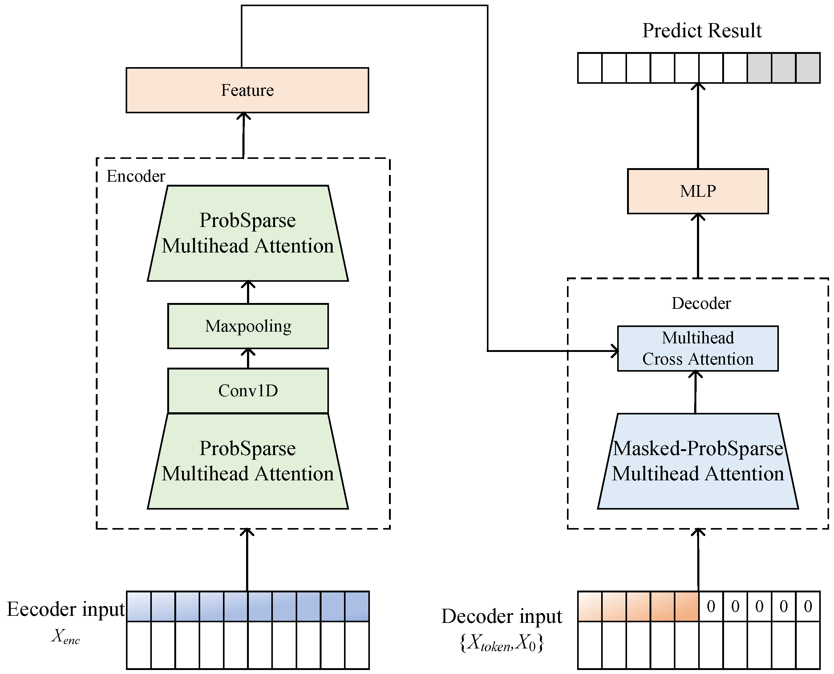
The Informer model is an enhancement of the Transformer model. It utilizes a Transformer-based encoder architecture but incorporates a ProbSparse Self-Attention mechanism, which reduces the computational time complexity and significantly shortens computation time. It also introduces a self-attention distilling mechanism, which adds one-dimensional convolutional and max-pooling layers to each self-attention block to further reduce the computational overhead. Furthermore, Informer employs a generative-style decoder that performs a single forward pass to generate all predicted outputs at once for long sequences, thereby greatly increasing the prediction speed for long time series. The architecture of the Informer is shown in Figure 2.

3.1.1. ProbSparse Self-Attention Mechanism

(1) The formula for the dot-product attention in the traditional self-attention mechanism is:
Attention ( Q , K , V ) = Softmax Q K d V
where Q is the matrix of query vectors, K is the matrix of key vectors, V is the matrix of value vectors, and d is the dimension of the input features.
(2) The traditional self-attention mechanism has a quadratic complexity, which leads to long computation times for long sequences. To address this issue, the ProbSparse self-attention mechanism defines the sparsity measurement for the i-th query by approximating the KL-divergence, dropping the constant term:
M ( q i , K ) = ln j = 1 L k e q i K j d 1 L k j = 1 L k q i K j d
where the first term is the Log-Sum-Exp (LSE) of the dot products of q i with all keys K j , and the second term is their arithmetic mean.
(3) By selecting only the queries with the highest sparsity scores to participate in the subsequent computation, the final attention is calculated as:
Attention ( Q , K , V ) = Softmax Q ¯ K d V
where Q ¯ is the matrix composed of the selected high-sparsity queries.

3.1.2. Self-Attention Distilling

To further reduce the computational overhead, the Informer encoder adds a one-dimensional convolutional layer and a max-pooling layer after each self-attention layer for a “distilling” operation:
X j + 1 = MaxPool ( ELU ( Conv 1 d ( [ X j ] AB ) ) )
where X j + 1 represents the output of the distilling operation from layer j to layer j + 1 , [ · ] AB denotes the output of the attention block, Conv1d is a one-dimensional convolution operation, ELU is the activation function, and MaxPool is the max-pooling operation.
When the convolutional layer distills features from the current layer to the next, the feature map is compressed to half its original length, further reducing computational costs while preserving the dominant features.

3.1.3. Generative-Style Decoder

Using a generative-style decoder, all output data points are generated in a single step, which significantly improves prediction efficiency. The input to the decoder is constructed as follows:
X de = Concat ( X token , X 0 ) R ( L token + L y ) × d model
where X de is the input vector for the decoder, X token R L token × d model is the start token, and X 0 R L y × d model is a placeholder for the target sequence to be predicted (typically filled with zeros).

3.2. CPO-Based VMD Parameter Optimization

To effectively address the non-stationarity and high-noise characteristics of stock price series, this paper adopts the “decomposition-prediction-ensemble” paradigm as the first step of its core strategy. Specifically, we employ Variational Mode Decomposition (VMD) to preprocess the original signal. However, the performance of VMD is highly dependent on its key parameters—the number of decomposed modes K and the quadratic penalty factor α —which are traditionally set based on experience or trial-and-error, making it difficult to guarantee optimality. To this end, this section proposes an adaptive VMD parameter optimization scheme based on the Crested Porcupine Optimizer (CPO) to ensure the effectiveness and robustness of the signal decomposition.

3.2.1. Variational Mode Decomposition (VMD) Principle

VMD is an advanced, adaptive, and non-recursive signal processing technique. Its core idea is to construct and solve a constrained variational problem to decompose a real-valued input signal x ( t ) into a series of discrete modal components u k ( t ) (i.e., Intrinsic Mode Functions, IMFs) with specific sparsity properties. Each mode u k is assumed to be an AM-FM signal that is compact around a center frequency ω k .
The optimization objective of VMD is to find K modal components such that the sum of their estimated bandwidths is minimized, subject to the constraint that the sum of these modes accurately reconstructs the original signal. This constrained variational problem is formulated as follows:
min u k , ω k k = 1 K t δ ( t ) + j π t u k ( t ) e j ω k t 2 2 s . t . k = 1 K u k ( t ) = x ( t )
where u k and ω k are the sets of K modal components and their respective center frequencies; t denotes the partial derivative with respect to time t; δ ( t ) is the Dirac delta function; j is the imaginary unit; and ∗ represents the convolution operation.
To solve the above problem, the constrained variational problem is transformed into an unconstrained one by introducing a quadratic penalty factor α and a Lagrange multiplier λ ( t ) . The augmented Lagrangian function L is defined as:
L ( u k , ω k , λ ) = α k = 1 K t δ ( t ) + j π t u k ( t ) e j ω k t 2 2 + x ( t ) k = 1 K u k ( t ) 2 2 + λ ( t ) , x ( t ) k = 1 K u k ( t )
This optimization problem can be solved iteratively using the Alternating Direction Method of Multipliers (ADMM). The modal components u ^ k , center frequencies ω k , and the Lagrange multiplier λ ^ are alternately updated in the frequency domain until a convergence criterion is met. The iterative update formulas are as follows:
u ^ k n + 1 ( ω ) = x ^ ( ω ) i k u ^ i n ( ω ) + λ ^ n ( ω ) 2 1 + 2 α ( ω ω k n ) 2 ω k n + 1 = 0 ω | u ^ k n + 1 ( ω ) | 2 d ω 0 | u ^ k n + 1 ( ω ) | 2 d ω λ ^ n + 1 ( ω ) = λ ^ n ( ω ) + τ x ^ ( ω ) k = 1 K u ^ k n + 1 ( ω )
where · ^ denotes the Fourier transform, and τ is an update parameter.

3.2.2. CPO-VMD Parameter Optimization Process

Although VMD has theoretical advantages, its decomposition effectiveness is extremely sensitive to the parameters K and α . To achieve adaptive parameter optimization, this paper introduces the Crested Porcupine Optimizer (CPO) algorithm. CPO is a metaheuristic algorithm that simulates the defensive behavior of crested porcupines against predators. It performs an efficient search in the solution space by simulating two mechanisms: the “scent strategy” (global exploration) and the “physical strategy” (local exploitation). This algorithm is characterized by its strong global search capability, fast convergence speed, and a reduced tendency to become trapped in local optima.
As illustrated in Figure 3, we formulate the VMD parameter search as an optimization task. The specific process is as follows:
  • Define the Fitness Function: We select Sample Entropy as the fitness function. Sample Entropy is a key metric for measuring the complexity of a time series; a smaller value indicates stronger regularity and lower noise levels. An ideal VMD decomposition should produce a series of stationary and physically meaningful modal components, which typically have low Sample Entropy values. Therefore, we set the average Sample Entropy of all modal components as the optimization objective. That is, the goal of the CPO algorithm is to find a set of parameters ( K , α ) that minimizes this fitness function.
  • Execute CPO Optimization: Within a predefined parameter range (e.g., K [ 2 , 10 ] , α [ 400 , 4000 ] ), the CPO algorithm searches for the optimal parameter combination by iteratively updating the population’s positions.
  • Sliding Decomposition Strategy: A critical aspect of our methodology is to strictly prevent data leakage. We perform CPO-VMD decomposition using a sliding window approach. While our model’s input sequence length (seq_len) is 96, we found that VMD requires a longer sequence for stable decomposition. Therefore, to generate the input for time t (which requires data from t 95 to t), we perform the decomposition on a longer preceding window of 960 time steps (i.e., the interval [ t 960 + 1 , t ] ). Crucially, from the resulting K decomposed IMFs (each of length 960), we only extract the final 96 time steps (the interval [ t 95 , t ] ) to serve as the input for the Informer network. This rolling decomposition ensures that at no point does the model use future information. For example, to predict from time 961, we decompose the series from time 1 to 960, and use the IMF segments from time 865 to 960 as input. This design assumes a ‘warm-up’ period of data (960 − 96 = 864 steps) is available before the first prediction.
Through this process, we find the most suitable decomposition parameters for each input sequence. To balance computational efficiency and specificity, we optimized these parameters per industry on the training set. We selected a representative company from each sector (e.g., AAPL for Information Technology, AFL for Financials, and ADM for Consumer Staples) to find a unified set of parameters for that sector. The parameters used in this study are as follows:
  • Information Technology:  K = 4 , α = 1111
  • Financials:  K = 4 , α = 1536
  • Consumer Staples:  K = 3 , α = 1625
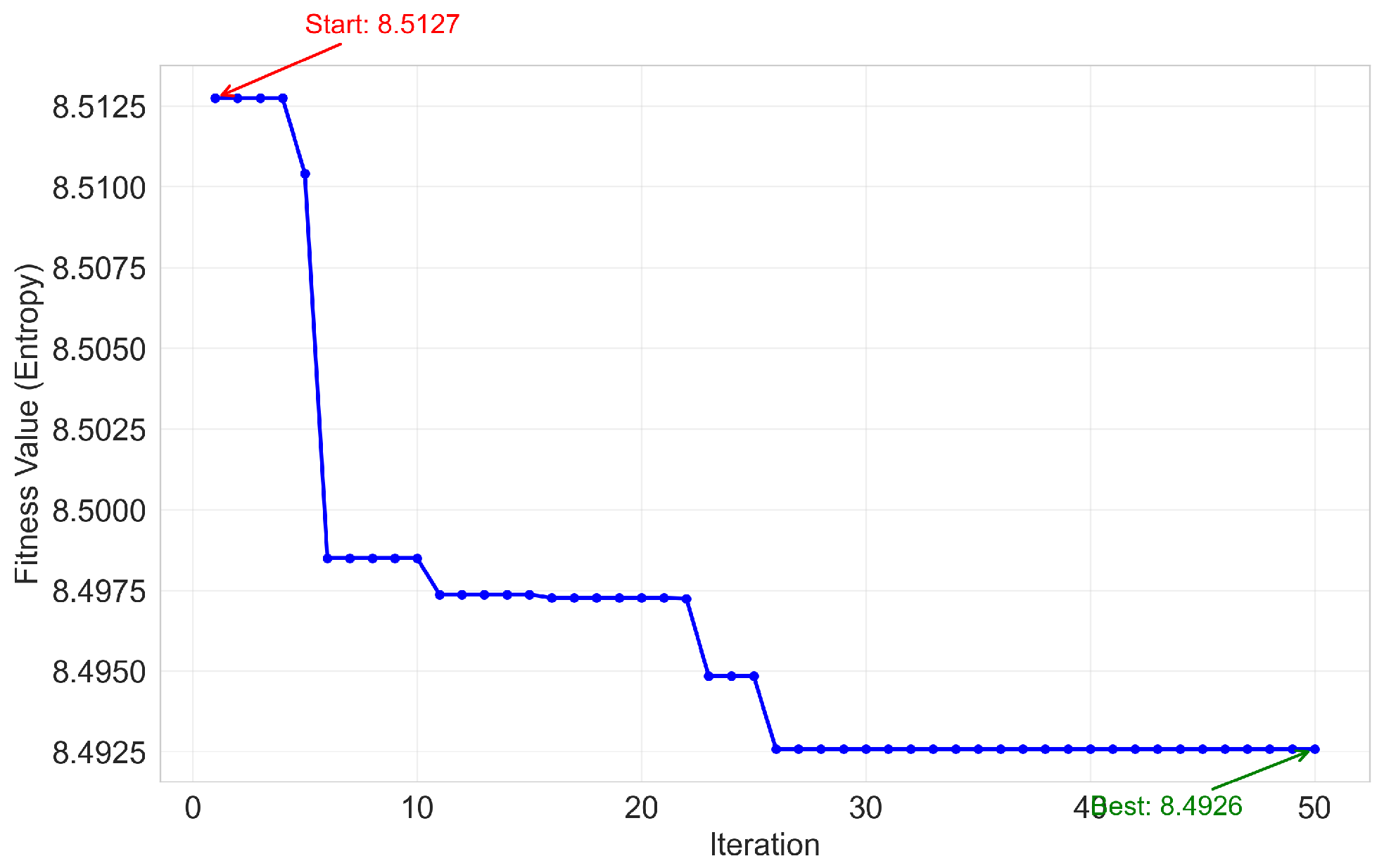
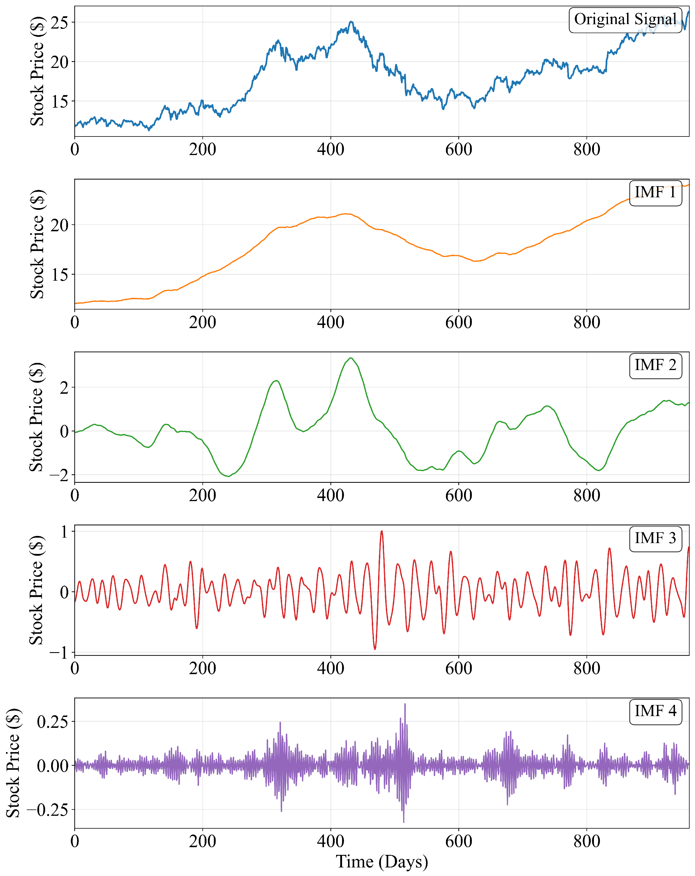
The convergence curve for the Information Technology sector optimization is shown in Figure 4. Figure 5 visualizes the decomposition result for an AAPL stock series using these parameters.

3.3. Multi-Scale Dilated Convolution

3.3.1. Fundamental Theory

Dilated Convolution, also known as Atrous Convolution (AConv), is a special type of convolution where a standard kernel is expanded by inserting a number of zeros (‘holes’) between consecutive values. It was first proposed in the Alogrithme à Trous for wavelet decomposition of time-varying signals and was later widely applied in semantic segmentation. The operation of AConv can be expressed as:
h ( i ) = k = 1 K d ( i + r × k ) · X ( k )
where d ( i ) is a one-dimensional discrete signal, h ( i ) is the i-th output feature value of d ( i ) after the dilated convolution operation, r is the dilation rate of the kernel, and K is the size of the kernel.
Global Average Pooling (GAP) refers to the operation of taking the spatial average of the output feature map from the last convolutional or pooling layer. Compared to fully-connected layers, a GAP layer has no parameters to train, thus significantly reducing the number of parameters and the computational load of the network. The GAP operation can be expressed as:
u c = 1 n i = 1 n v i c
where c is the number of output channels, v i c is the i-th feature value in the c-th channel, n is the number of feature values per channel, and u c is the global average value output for the c-th channel.
Batch Normalization (BN) can reduce the distribution difference between the features of training and testing samples, thereby improving the network’s performance and generalization ability. The BN operation, when placed after a convolutional layer, can be expressed as:
z i = x i μ B σ B 2 + ε , y i = γ z i + β
where x i is the i-th value of the input feature map in layer l; μ B is the mean of the input samples in each batch; σ B 2 is the variance of the input samples in each batch; ε is a small constant to prevent division by zero; z i is the i-th value of the standardized feature map in layer l; γ and β are the scale and shift factors, respectively; and y i is the i-th output result of batch normalization in layer l.

3.3.2. Multi-Scale Dilated Convolution Module

First, standard convolutional kernels and dilated convolutional kernels of different sizes are applied to the input layer of the model to fully extract features at various scales from different receptive fields. Then, each of the three large-kernel convolutional layers is followed by a small 1 × 1 convolutional kernel to further integrate the features extracted by the large kernels in each channel, as shown in Figure 6.
(1) The mathematical form of the multi-scale convolution is:
g k i = Conv k i ( X , W k i ) + b k i
where X is the input feature, W k i is the i-th kernel of size k, b k i is the bias added to the output feature of the i-th kernel of size k, g k i is the i-th output feature from the kernel of size k, and Conv is the convolution operation.
(2) The feature maps output by the 1 × 1 small-kernel convolutions are processed with Batch Normalization according to Equation (11).
(3) A non-linear mapping is applied to the normalized output features to enhance their expressive power and separability. This paper uses the commonly adopted Rectified Linear Unit (ReLU) as the activation function, whose mathematical form is:
y i = f ( α i ) = max ( 0 , α i )
where α i is the i-th value of the input feature map in layer l after being normalized by Equation (11), and y i is the i-th output result of α i in layer l after ReLU activation.
(4) A Max Pooling (MaxPool) operation is performed on the features output after ReLU activation. Its mathematical form is:
p i l + 1 = max t S ( q i l ( t ) )
where q i l ( t ) is the output of the t-th neuron in the i-th channel of layer l, S is the size of the pooling kernel, and p i l + 1 is the output result of the i-th channel in layer l + 1 .
(5) The feature maps extracted by the convolutions at three different scales are denoted as X 1 , X 2 , and X 3 . They are then stacked along the depth dimension using tensor concatenation to achieve feature fusion. The mathematical form of this feature stacking is:
Y = concat ( X 1 , X 2 , X 3 )
where concat is the tensor concatenation operation, and Y is the output result of stacking X 1 , X 2 , and X 3 . The final fused and distilled features are then input into the Informer’s decoder.

4. Experiments

4.1. Dataset

The experimental data for this study is sourced from the constituent stocks of the S&P 500 index. We selected a time span from 3 January 2011, to 12 December 2022. The data is sampled at a daily frequency (one data point per trading day), and we filtered for 352 companies with complete data during this period. To test the model’s generalization ability and its adaptability to different market dynamics, we categorized these companies into three representative sectors based on the Global Industry Classification Standard (GICS) [25]:
  • Information Technology: This sector is typically characterized by high growth and is sensitive to market risk appetite. Its stock price dynamics are well-described by features such as momentum, earnings forecast revisions, and R&D intensity.
  • Financials: This sector is highly sensitive to interest rate changes. Its performance is closely correlated with exogenous factors like macroeconomic policies (e.g., policy rates), market interest rates (e.g., long- and short-term government bond yields), and credit spreads.
  • Consumer Staples: This sector possesses defensive characteristics. Companies in this sector have relatively stable earnings and lower volatility, often exhibiting strong downside resistance during market-wide drawdowns.
The stock price prediction task is formulated as a multivariate time series regression problem, where we use historical data from the past 96 time steps to predict the closing price for the next 48 time steps. To construct a rich feature representation, the model’s input includes basic trading data such as opening price (OPEN), closing price (CLOSE), highest price (HIGH), lowest price (LOW), and trading volume (VOLUME), as well as multiple quantitative technical factors from the ‘mytt’ factor library. These factors are grouped into three categories to comprehensively capture market dynamics: (1) Trend-following factors, such as the MACD series (DIF, DEA, MACD) and Bollinger Bands (UPPER, MID, LOWER), to identify the market’s primary direction and long-term trends; (2) Momentum/Oscillator factors, such as the Stochastic Oscillator (KDJ), Bias Ratio (BIAS), Commodity Channel Index (CCI), and Momentum (MTM), to capture short-term overbought/oversold signals and pullback opportunities; and (3) Sentiment factors, such as the Psychological Line (PSY), Popularity Index (AR), and Willingness to Buy/Sell Index (BR), to quantify the collective psychological state of market participants and assist in identifying market turning points. The specific factors are detailed in Table 1. By jointly utilizing these factors from different dimensions, the model can obtain a more comprehensive understanding of the market state. All input data is subjected to Z-score normalization before being fed into the model. To prevent data leakage, the mean and standard deviation required for normalization are computed only on the training dataset. These statistics are then saved and applied consistently to normalize the validation and test datasets.

4.2. Baseline Models

To validate the effectiveness of the framework proposed in this paper, we selected several state-of-the-art time series forecasting models as baselines for comparison:
  • Transformer [26]: This architecture employs a self-attention mechanism and an encoder-decoder structure, supporting parallel processing of sequential data to effectively capture long-range dependencies. However, its quadratic time/memory complexity ( O ( L 2 ) ) limits its direct application in long-sequence time series forecasting.
  • Autoformer [18]: A decomposition-based Transformer with an auto-correlation mechanism for long-term time series forecasting. The model incorporates a series decomposition block as a built-in operator to progressively separate trend-cyclical and seasonal components. The auto-correlation mechanism replaces self-attention, mining sub-series dependencies based on periodicity via Fast Fourier Transform and aggregating similar sub-series. It has achieved state-of-the-art performance on datasets for energy, traffic, and weather.
  • Informer [10]: An efficient Transformer for long-sequence time series forecasting. The model addresses the limitations of the Transformer through three innovations: ProbSparse self-attention, self-attention distilling, and a generative-style decoder. It outperforms traditional models on large-scale datasets such as ETT and Traffic.
  • Informer-CGRU [27]: A model based on Informer for non-stationary time series forecasting. It introduces multi-scale causal convolutions to capture causal relationships across time scales and uses a GRU layer to re-learn causal features, enhancing robustness to non-linearity and high noise.
  • iTransformer [28]: An inverted Transformer architecture optimized for time series forecasting. This model improves the input processing and attention mechanism of the Transformer to enhance temporal pattern capturing. By reformulating the attention computation paradigm, it improves the efficiency of modeling long-range dependencies in time series data.
  • FEDformer [19]: A frequency-enhanced decomposition Transformer for long-term forecasting. The model integrates seasonal-trend decomposition with frequency-domain transforms. Frequency-enhanced blocks and attention mechanisms replace self-attention and cross-attention, ensuring linear complexity by randomly selecting frequency components. This model improves the distributional consistency between predicted and true sequences.
  • DAT-PN [29]: A Transformer-based dual-attention framework for financial time series forecasting. The framework consists of two parallel networks: a Price Attention Network (PAN) processes historical price data using multi-head masked self-attention (MMSA) and multi-head cross-attention (MCA) to capture temporal dependencies, while a Non-price Attention Network uses a convolutional LSTM, a bidirectional GRU, and self-attention to extract features from non-price financial data.
  • VLTCNA [12]: A stock sequence prediction model that integrates Variational Mode Decomposition (VMD) with dual-channel attention. VMD decomposes the stock sequence into stable frequency sub-windows using a sliding window to reduce volatility. A dual-channel network (LSTMA + TCNA) comprises an LSTMA (2 LSTM layers + self-attention) and a TCNA (4 F-TCN modules + self-attention), where the former captures long-term dependencies and the latter captures local/short-term patterns.

4.3. Experimental Environment and Parameter Settings

4.3.1. Experimental Environment

The specific settings for the experimental environment are shown in Table 2:

4.3.2. Hyperparameter Settings

The specific hyperparameter settings for the experiment are shown in Table 3:
The key hyperparameters listed in Table 3, as well as the specific parameters for the MDCM module, were determined using a grid search on the validation set of the Information Technology dataset. The search space and final choices for the MDCM module and other key network parameters are detailed in Table 4.

4.4. Evaluation Metrics

The experiments use Mean Absolute Error (MAE), Mean Squared Error (MSE), and Root Mean Squared Error (RMSE) as performance evaluation metrics. A smaller value for these metrics indicates a smaller prediction error and better model performance. The calculation methods for these metrics are as follows.
MAE = 1 m i = 1 m | y i y ^ i |
MSE = 1 m i = 1 m ( y i y ^ i ) 2
RMSE = 1 m i = 1 m ( y i y ^ i ) 2
where m is the number of evaluation samples, y i is the true value, and y ^ i is the predicted value. MAE represents the average of the absolute differences between predicted and true values and is equally sensitive to large and small errors, focusing on the overall model performance. MSE represents the average of the squared differences between predicted and actual values and is more sensitive to large errors. RMSE is the square root of MSE, sharing the same units as the target variable, which allows for a more intuitive interpretation of the error. The smaller the values of these metrics, the smaller the corresponding error and the better the model’s performance.

4.5. Comparative Analysis of Experiments

To validate the effectiveness of our proposed model, we selected several recent state-of-the-art methods as baseline models for comparison on three different industry datasets from the S&P 500.
The results of the comparative experiments are shown in Table 5. The best results for each metric are marked in bold, and the second-best results are underlined. As can be seen from the table, our proposed method achieves optimal or near-optimal performance across the three different industry datasets.
As the table indicates, our proposed method achieves optimal or near-optimal performance across the three different industry datasets. Specifically: In the highly volatile “Information Technology” sector, where stock prices typically contain more high-frequency noise and abrupt changes, our model achieved the best performance on the MSE and RMSE metrics (0.1411 and 0.3760, respectively). Compared to the second-best model, iTransformer, the MSE was reduced by 5.24%. This suggests that the CVASD module successfully separated high-frequency noise from the main trends, allowing the model to focus more on learning effective information. Simultaneously, the MDCM module, with its multi-scale receptive fields, effectively captured fluctuation characteristics across different periods, leading to outstanding performance on the MSE metric, which penalizes larger errors more heavily. In the “Financials” sector, which is closely linked to the macro-economy and exhibits stronger cyclical patterns, our model achieved the best results across all metrics, with MAE, MSE, and RMSE values of 0.3380, 0.1809, and 0.4279, respectively. Compared to the second-best model, DAT-PN, the MSE was reduced by 5.29%. This demonstrates the effectiveness of the proposed framework in handling sequences with complex cyclical components, where the adaptive decomposition and multi-scale feature extraction prove highly beneficial. For the “Consumer Staples” sector, where stock price movements are relatively stable and more trend-driven, our model also demonstrated comprehensive superiority, ranking first on all metrics. Compared to the second-best model, FEDformer, the MSE was reduced by 6.35%, showing the most significant advantage. This indicates that even in scenarios with relatively low noise and clear trends, our model can uncover subtle patterns that are difficult for a single model to capture, thanks to its fine-grained signal decomposition and multi-scale feature extraction, thereby achieving more accurate predictions. In summary, the proposed CVASD-MDCM-Informer model exhibits excellent performance and good generalization ability across financial time series with different characteristics, validating the effectiveness of combining adaptive signal decomposition with multi-scale feature extraction.

4.6. Ablation Study

To verify the effectiveness of the key modules in our model, we designed an ablation study. The experiment evaluates the contribution of specific components to the overall performance by removing them, as shown in Table 6. “w/o” indicates the removal of the corresponding module; bold text indicates the best (lowest) value for that metric within that industry.
From the experimental data in Table 6, it is evident that the complete model (Our Model) significantly outperforms all other variants in the tests across all three industries, achieving the lowest prediction errors for MAE, MSE, and RMSE. In contrast, the original Informer, serving as the baseline model (w/o CVASD & MDCM), performed the worst. For instance, on the Information Technology dataset, the full model reduced MAE, MSE, and RMSE by 19.7%, 30.4%, and 19.5%, respectively, compared to the baseline. This strongly demonstrates that the combination of our two proposed improvement modules can effectively enhance the accuracy of stock price prediction, validating the rationality and advancement of the overall model design.
When the CVASD module was removed (w/o CVASD), the model’s performance showed a significant decline compared to the complete model. This was observed across all datasets, particularly in the Information Technology sector, where removing this module led to a 10.3% increase in MAE. The core function of the CVASD module is to decompose the high-noise, non-stationary original stock price series into a set of more predictable modal components with distinct frequency characteristics. The experimental results show that this “decomposition-prediction-aggregation” strategy can effectively filter market noise and help the model more accurately capture underlying patterns at different time scales, which is crucial for improving prediction stability.
Similarly, removing the MDCM module (w/o MDCM) also led to a decrease in the model’s predictive capability. The MDCM endows the model with the ability to capture multi-scale temporal dependencies within a single layer by using parallel convolutional kernels with different dilation rates. Compared to the standard convolutions in the original Informer, this design allows for a more comprehensive extraction of both short-term details and long-term trend features from the sequence. The experimental results validate the effectiveness of this design, proving that enhancing the local feature extraction capability at the encoder end is essential for improving overall prediction accuracy.
By comparing the two variants with a single module removed, we observe that the modules exhibit differential importance across different industry datasets. In the Information Technology sector, the performance loss from removing the CVASD module was greater than that from removing the MDCM module, which may imply that noise interference and multi-frequency superposition characteristics in this sector’s stock series are the main challenges for prediction. In the Financials sector, however, the impact of removing the MDCM module was more significant, suggesting that accurately capturing complex long- and short-term temporal dependencies is key to forecasting in this domain. In the Consumer Staples sector, removing the CVASD module had a larger impact on MSE and RMSE, while removing the MDCM module had a larger impact on MAE. This reveals that CVASD plays a prominent role in suppressing extreme errors (which are amplified by the squared term in MSE/RMSE), whereas MDCM contributes more to improving the overall average prediction accuracy (as measured by MAE).
In conclusion, the results of the ablation study clearly demonstrate that both the CVASD and MDCM modules are indispensable components of our prediction framework. They optimize the model from the perspectives of signal processing and feature extraction, respectively, and through their synergistic effect, significantly enhance the model’s predictive performance and robustness when handling complex financial time series.

5. Conclusions and Future Work

This paper proposed a novel hybrid framework, CVASD-MDCM-Informer, for stock price prediction, designed to address the challenges of high noise and non-stationarity in financial time series. Our ‘decomposition-prediction-ensemble’ approach first utilizes a CVASD module, where the CPO algorithm adaptively optimizes VMD parameters (K and α ) to decompose the raw price series into more stable IMF components. Subsequently, an MDCM module with parallel dilated convolutions replaces the standard convolution in the Informer, enhancing the model’s ability to capture multi-scale features from these components.
Extensive experiments on three S&P 500 industry datasets (Information Technology, Financials, and Consumer Staples) demonstrated the superiority of our framework. Compared to several state-of-the-art baseline models, including iTransformer, FEDformer, and DAT-PN, our model achieved significant improvements across all evaluation metrics (MAE, MSE, RMSE). Ablation studies further confirmed the indispensable contributions of both the CVASD and MDCM modules, validating our hypothesis that combining adaptive signal decomposition with multi-scale feature extraction is a highly effective strategy for complex time series forecasting.

5.1. Limitations

Despite the promising results, this study has several limitations that should be acknowledged.
  • Survivorship Bias: As noted by the reviewer, our dataset construction, which selected 352 companies with complete data from 2011 to 2022, introduces survivorship bias. By excluding delisted or inactive firms, our sample is skewed towards more stable and successful companies, which may artificially inflate the model’s predictability. Future work should explore methods to incorporate data from delisted stocks to create a more representative dataset.
  • Computational Overhead and Data Requirement: The CPO-VMD rolling decomposition strategy, while effective, is computationally intensive. Furthermore, our use of a 960-step window for stable decomposition requires a significant ‘warm-up’ period (864 data points in our study), making the model less suitable for ‘cold-start’ scenarios or very short time series.

5.2. Future Work

Building on this work, several avenues for future research are apparent.
  • Broader Asset Classes: The framework’s effectiveness should be tested on other financial instruments, such as exchange-traded funds (ETFs), cryptocurrencies, and macroeconomic indicators, which possess different volatility structures and noise characteristics.
  • Cross-Domain Applications: The proposed methodology is not limited to finance. It can be extended to other domains characterized by complex, non-stationary time series, such as energy load forecasting, electricity price prediction, and meteorological forecasting.
  • Model Efficiency: Future research could explore more lightweight adaptive decomposition techniques or investigate knowledge distillation methods to reduce the computational burden of the CVASD module without sacrificing performance.

Author Contributions

Conceptualization, J.S.; Methodology, J.S. and R.Y.K.L.; Software, J.S., Y.D. and J.Y.; Validation, J.S. and J.Y.; Writing—original draft, J.S. and Y.D.; Visualization, J.S., Y.D. and H.Z. All authors have read and agreed to the published version of the manuscript.

Funding

This work was partly supported by a grant from the Research Grants Council of the Hong Kong SAR (Project No.: CityU 11507323).

Data Availability Statement

The relevant data can be obtained by contacting the corresponding author.

Conflicts of Interest

The authors declare that they have no known competing financial interests or personal relationships that could have appeared to influence the work reported in this paper.

References

  1. Rezaei, H.; Faaljou, H.; Mansourfar, G. Stock price prediction using deep learning and frequency decomposition. Expert Syst. Appl. 2021, 169, 114332. [Google Scholar] [CrossRef]
  2. Hossein, A.; Charlotte, C.; Hou, A.J. The effect of uncertainty on stock market volatility and correlation. J. Bank. Financ. 2023, 154, 106929. [Google Scholar]
  3. Su, J.; Lau, R.Y.K.; Yu, J.; NG, D.C.T.; Jiang, W. A multi-modal data fusion approach for evaluating the impact of extreme public sentiments on corporate credit ratings. Complex Intell. Syst. 2025, 11, 436. [Google Scholar] [CrossRef]
  4. Barberis, N.; Jin, L.J.; Wang, B. Prospect theory and stock market anomalies. J. Financ. 2021, 76, 2639–2687. [Google Scholar] [CrossRef]
  5. Peress, J.; Schmidt, D. Noise traders incarnate: Describing a realistic noise trading process. J. Financ. Mark. 2021, 54, 100618. [Google Scholar] [CrossRef]
  6. Farahani, M.S.; Hajiagha, S.H.R. Forecasting stock price using integrated artificial neural network and metaheuristic algorithms compared to time series models. Soft Comput. 2021, 25, 8483. [Google Scholar] [CrossRef] [PubMed]
  7. Suthaharan, S. Support vector machine. In Machine Learning Models and Algorithms for Big Data Classification: Thinking with Examples for Effective Learning; Springer: Berlin/Heidelberg, Germany, 2016; pp. 207–235. [Google Scholar]
  8. Medsker, L.; Jain, L.C. Recurrent Neural Networks: Design and Applications; CRC Press: Boca Raton, FL, USA, 1999. [Google Scholar]
  9. Nagar, P.; Shastry, K.; Chaudhari, J.; Arora, C. SEMA: Semantic Attention for Capturing Long-Range Dependencies in Egocentric Lifelogs. In Proceedings of the IEEE/CVF Winter Conference on Applications of Computer Vision, Waikoloa, HI, USA, 3–8 January 2024; pp. 7025–7035. [Google Scholar]
  10. Zhou, H.; Zhang, S.; Peng, J.; Zhang, S.; Li, J.; Xiong, H.; Zhang, W. Informer: Beyond efficient transformer for long sequence time-series forecasting. In Proceedings of the AAAI Conference on Artificial Intelligence, Virtually, 2–9 February 2021; Volume 35, pp. 11106–11115. [Google Scholar]
  11. Zhang, C.; Sjarif, N.N.A.; Ibrahim, R. Deep learning models for price forecasting of financial time series: A review of recent advancements: 2020–2022. Wiley Interdiscip. Rev. Data Min. Knowl. Discov. 2024, 14, e1519. [Google Scholar] [CrossRef]
  12. Liu, Y.; Huang, S.; Tian, X.; Zhang, F.; Zhao, F.; Zhang, C. A stock series prediction model based on variational mode decomposition and dual-channel attention network. Expert Syst. Appl. 2024, 238, 121708. [Google Scholar] [CrossRef]
  13. Ma, R.; Han, T.; Lei, W. Cross-domain meta learning fault diagnosis based on multi-scale dilated convolution and adaptive relation module. Knowl.-Based Syst. 2023, 261, 110175. [Google Scholar] [CrossRef]
  14. Dragomiretskiy, K.; Zosso, D. Variational mode decomposition. IEEE Trans. Signal Process. 2013, 62, 531–544. [Google Scholar] [CrossRef]
  15. Abdel-Basset, M.; Mohamed, R.; Abouhawwash, M. Crested Porcupine Optimizer: A new nature-inspired metaheuristic. Knowl.-Based Syst. 2024, 284, 111257. [Google Scholar] [CrossRef]
  16. Zhang, Z.; Liu, Q.; Hu, Y.; Liu, H. Multi-feature stock price prediction by LSTM networks based on VMD and TMFG. J. Big Data 2025, 12, 74. [Google Scholar] [CrossRef]
  17. Jain, A.; Zamir, A.R.; Savarese, S.; Saxena, A. Structural-rnn: Deep learning on spatio-temporal graphs. In Proceedings of the IEEE Conference on Computer Vision and Pattern Recognition, Las Vegas, NV, USA, 26 June–1 July 2016; pp. 5308–5317. [Google Scholar]
  18. Wu, H.; Xu, J.; Wang, J.; Long, M. Autoformer: Decomposition transformers with auto-correlation for long-term series forecasting. Adv. Neural Inf. Process. Syst. 2021, 34, 22419–22430. [Google Scholar]
  19. Zhou, T.; Ma, Z.; Wen, Q.; Wang, X.; Sun, L.; Jin, R. Fedformer: Frequency enhanced decomposed transformer for long-term series forecasting. In Proceedings of the International Conference on Machine Learning, PMLR, Baltimore, MD, USA, 17–23 July 2022; pp. 27268–27286. [Google Scholar]
  20. Lv, P.; Shu, Y.; Xu, J.; Wu, Q. Modal decomposition-based hybrid model for stock index prediction. Expert Syst. Appl. 2022, 202, 117252. [Google Scholar] [CrossRef]
  21. Gao, Z.; Zhang, J. The fluctuation correlation between investor sentiment and stock index using VMD-LSTM: Evidence from China stock market. N. Am. J. Econ. Financ. 2023, 66, 101915. [Google Scholar] [CrossRef]
  22. Li, Q.; Wang, G.; Wu, X.; Gao, Z.; Dan, B. Arctic short-term wind speed forecasting based on CNN-LSTM model with CEEMDAN. Energy 2024, 299, 131448. [Google Scholar] [CrossRef]
  23. Rayi, V.K.; Mishra, S.; Naik, J.; Dash, P.K. Adaptive VMD based optimized deep learning mixed kernel ELM autoencoder for single and multistep wind power forecasting. Energy 2022, 244, 122585. [Google Scholar] [CrossRef]
  24. Ding, J.; Huang, L.; Xiao, D.; Li, X. GMPSO-VMD algorithm and its application to rolling bearing fault feature extraction. Sensors 2020, 20, 1946. [Google Scholar] [CrossRef]
  25. S&P Global Market Intelligence. The Global Industry Classification Standard (GICS®); Technical Report; Standard & Poor’s Financial Services LLC (S&P), MSCI: New York, NY, USA, 2018. [Google Scholar]
  26. Vaswani, A.; Shazeer, N.; Parmar, N.; Uszkoreit, J.; Jones, L.; Gomez, A.N.; Kaiser, L.; Polosukhin, I. Attention Is All You Need. arXiv 2023, arXiv:1706.03762. [Google Scholar] [CrossRef]
  27. Yang, Y.; Dong, Y. Informer_Casual_LSTM: Causal Characteristics and Non-Stationary Time Series Prediction. In Proceedings of the 2024 7th International Conference on Machine Learning and Natural Language Processing (MLNLP), Chengdu, China, 18–20 October 2024; IEEE: Piscataway, NJ, USA, 2024; pp. 1–6. [Google Scholar]
  28. Liu, Y.; Hu, T.; Zhang, H.; Wu, H.; Wang, S.; Ma, L.; Long, M. itransformer: Inverted transformers are effective for time series forecasting. arXiv 2023, arXiv:2310.06625. [Google Scholar]
  29. Hadizadeh, A.; Tarokh, M.J.; Ghazani, M.M. A novel transformer-based dual attention architecture for the prediction of financial time series. J. King Saud Univ. Comput. Inf. Sci. 2025, 37, 72. [Google Scholar] [CrossRef]
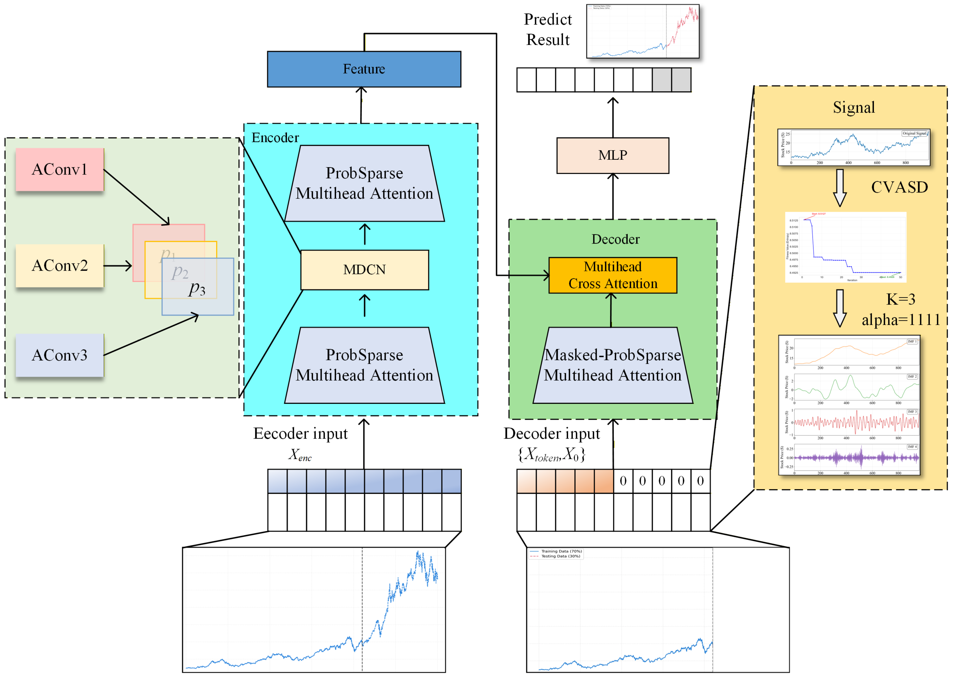
Figure 1. The overall architecture of the proposed CVASD-MDCM-Informer framework. The process follows a ‘decomposition-prediction-ensemble’ paradigm: (1) The original stock series is decomposed into K IMFs by the CVASD module. (2) Each IMF is fed into a shared-weight Informer encoder, which uses the MDCM module for multi-scale feature extraction. (3) The decoder predicts the future 48 steps for each IMF. (4) The final prediction is obtained by aggregating the results from all IMFs.
Applsci 15 12450 g001
Figure 2. The standard Informer architecture [10], serving as the backbone of our model. It features an encoder with ProbSparse self-attention and distilling, and a generative decoder for efficient long-sequence forecasting.
Applsci 15 12450 g002
Figure 3. Flowchart of the CPO-VMD signal decomposition process. For each rolling window of data, the CPO algorithm iteratively searches for the optimal VMD parameters ( K , α ) by minimizing the average sample entropy (the fitness function) of the resulting IMFs.
Applsci 15 12450 g003
Figure 4. Convergence curve of the fitness function (Average Sample entropy) during the CPO algorithm optimization process for the AAPL dataset (Information Technology sector). The algorithm rapidly converges to a stable minimum value, demonstrating its efficiency in finding optimal VMD parameters.
Applsci 15 12450 g004
Figure 5. Example of CPO-VMD decomposition results for the AAPL stock price series (Information Technology sector). The original complex series (top) is decomposed into four distinct modal components (IMF1 to IMF4) with frequencies ranging from high (IMF1, capturing noise) to low (IMF4, capturing the main trend).
Applsci 15 12450 g005
Figure 6. The architecture of the proposed Multi-scale Dilated Convolution Module (MDCM). It replaces the standard 1D convolution in Informer. Input features are processed in parallel by three branches with different dilation rates (e.g., 1, 2, 4) to capture dependencies at multiple time scales. The outputs are concatenated to produce a rich, multi-scale feature representation.
Applsci 15 12450 g006
Table 1. Quantitative Factors.
Factor TypeFactor Name
Basic FactorsOPEN, CLOSE, HIGH, LOW, VOLUME
DIF, DEA, MACD
KDJ, BIAS1, BIAS2, BIAS3,
Technical FactorsUPPER, MID, LOWER,
PSY, PSYMA, CCI,
MTM, MTMMA, AR, BR
Table 2. Experimental Environment Settings.
Environment ComponentSpecification
Runtime EnvironmentPython 3.7
Deep Learning FrameworkPytorch 1.9.1 + CUDA 11.1
Operating SystemWindows 10
CPU ModelIntel Core i7-12700K @ 4.9 GHz
Memory (RAM)64 GB (4 × 16 GB) DDR4 @ 3600 MHz
GPU ModelNVIDIA GeForce RTX 3090 (24 GB)
Table 3. Hyperparameter Settings.
Parameter NameDescriptionValue
batch_sizeBatch Size64
learn_rateLearning Rate0.0001
seq_lenInput Sequence Length96
label_lenLabel Sequence Length48
pred_lenOutput Sequence Length48
factorSparsity Factor5
n_headsNumber of Attention Heads8
e_layersNumber of Encoder Layers2
d_layersNumber of Decoder Layers1
d_modelModel Dimension512
Table 4. Grid search space and selected hyperparameters for key network parameters.
ParameterSearch SpaceSelected Value
Learning rate{0.0001, 0.0005, 0.001}0.0001
Batch size{32, 64, 128}64
Encoder layers ( e _ l a y e r s ){2, 3, 4}2
MDCM kernel sizes{(1, 3, 5), (3, 5, 7), (1, 5, 9)}(3, 5, 7)
MDCM dilation rates{(1, 2, 4), (1, 3, 5), (1, 4, 8)}(1, 2, 4)
Model dimension ( d _ model ){256, 512}512
Table 5. Comparative experimental results.
ModelMetricInformation TechFinancialsConsumer Staples
TransformerMAE0.39770.39780.3378
MSE0.22280.23800.2089
RMSE0.47280.49100.4690
AutoformerMAE0.38450.42400.3776
MSE0.23950.23980.2067
RMSE0.48900.48890.4677
InformerMAE0.37270.40110.3578
MSE0.20240.23860.1890
RMSE0.45030.48760.4335
Informer-CGRUMAE0.33780.36580.3349
MSE0.17010.22100.1779
RMSE0.41250.46130.4212
iTransformerMAE0.30890.36780.3581
MSE0.14890.21830.1852
RMSE0.38520.46730.4398
DAT-PNMAE0.33890.35080.3238
MSE0.17710.19100.1681
RMSE0.42090.43840.4230
FEDformerMAE0.32940.35850.3224
MSE0.16440.19940.1448
RMSE0.40870.44700.3843
VLTCNAMAE0.32680.37150.3231
MSE0.16170.20940.1767
RMSE0.41030.45640.4109
OursMAE0.31100.33800.2942
MSE0.14110.18090.1356
RMSE0.37600.42790.3722
ImprovementMAE−0.68%3.65%8.74%
MSE5.24%5.29%6.35%
RMSE2.39%2.40%3.15%
Table 6. Ablation study results across industries (lower is better).
IndustryVariantMAEMSERMSE
Information Technologyw/o CVASD & MDCM0.38740.20280.4672
w/o CVASD0.34320.17450.4262
w/o MDCM0.32340.16700.4003
Our Model0.31100.14110.3760
Financialsw/o CVASD & MDCM0.37890.22570.4766
w/o CVASD0.35370.19090.4460
w/o MDCM0.35810.21360.4578
Our Model0.33800.18090.4279
Consumer Staplesw/o CVASD & MDCM0.36730.18300.4335
w/o CVASD0.31040.16890.4031
w/o MDCM0.32070.15890.3899
Our Model0.29420.13560.3722
Disclaimer/Publisher’s Note: The statements, opinions and data contained in all publications are solely those of the individual author(s) and contributor(s) and not of MDPI and/or the editor(s). MDPI and/or the editor(s) disclaim responsibility for any injury to people or property resulting from any ideas, methods, instructions or products referred to in the content.