Article

Iterative Forecasting of Short Time Series

by
Evangelos Bakalis
Department of Chemistry “G. Ciamician”, University of Bologna, V. P. Gobetti 85, 40129 Bologna, Italy
Appl. Sci. 2025, 15(21), 11580; https://doi.org/10.3390/app152111580
Submission received: 29 September 2025 / Revised: 25 October 2025 / Accepted: 27 October 2025 / Published: 29 October 2025
(This article belongs to the Special Issue Advanced Methods for Time Series Forecasting)

Abstract

We forecast short time series iteratively using a model based on stochastic differential equations. The recorded process is assumed to be consistent with an α -stable Lévy motion. The generalized moments method provides the values of the scaling exponent and the parameter α , which determine the form of the stochastic term at each iteration. Seven weekly recorded economic time series—the DAX, CAC, FTSE100, MIB, AEX, IBEX, and STOXX600—were examined for the period from 2020 to 2025. The parameter α is always 2 for the four of them, FTSE100, AEX, IBEX, and STOXX600, indicating quasi-Gaussian processes. For FTSE100, IBEX, and STOXX600, the processes are anti-persistent (H < 0.5).The rest of the examined markets show characteristics of uncorrelated processes whose values are drawn from either a log-normal or a log-Lévy distribution. Further, all processes are multifractal, as the non-zero value of the mean intermittency indicates. The model’s forecasts, with the time horizon always one-step-ahead, are compared to the forecasts of a properly chosen ARIMA model combined with Monte Carlo simulations. The low values of the absolute percentage error indicate that both models function well. The model’s outcomes are further compared to ARIMA forecasts by using the Diebold–Mariano test, which yields a better forecast ability for the proposed model since it has less average loss. The ability and accuracy of the model to forecast even small time series is further supported by the low value of the absolute percentage error; the value of 4 serves as an upper limit for the majority of the forecasts.

1. Introduction

In diverse fields, processes are typically presented as time series; therefore, it would be very beneficial, if it is feasible through the available data, to forecast the evolution of such a process and make well-informed decisions [1]. The experimental evidence can be categorized as stochastic, noisy deterministic, deterministic, or a combination of these. Among deterministic data, those that show chaotic dynamics are important since they display very complex trajectories [2]. A finite-size trajectory can be either stochastic or chaotic since both are very much alike; hence, data pre-processing will be crucial [3]. Stochastic data can be correlated or uncorrelated in time, a property usually revealed, but not limited by, the form of their power spectra over the frequency domain [4].
A flat power spectrum indicates the existence of a memory-less stochastic process—white noise. However, the probability distribution from which such a process draws values is to be determined [5]. The power spectrum obeys a power law of the form S ( f ) f β , with f being the frequency and β the scaling exponent. A link has been established between the scaling exponent of the spectrum and the scaling exponent H of the process, which is called the Hurst exponent in honor of Harold Edwin Hurst. More specifically, for stationary processes, β = 2 H 1 with 1 < β < 1 , and β = 2 H + 1 with 1 < β < 3 for the non-stationary [6,7]. Hurst, in his seminal work ref. [8], introduced the adjusted range statistics. Later, Mandelbrot and Wallis established the mathematical foundation for the rescaled range analysis (R/S) that is used today through a heuristic graphical method [9]. They demonstrated how a scaling property for stationary processes permits a link between past and future events. Let x ( t ) be a stationary time series, and let τ be the length of the window connecting the differences between past and future events. If there is a unique scaling, the equation x ( τ ) = c τ H holds; note that c is a positive constant and H is the scaling exponent, H ( 0 , 1 ) . For 0 < H < 1 2 , the process is anti-persistent, meaning that every new value is likely to go in the opposite direction of the previous one. For 1 2 < H < 1 , the process is called persistent, and every new value is likely to follow the trajectory of the previous one. For H = 1 2 , the process has no memory, and every new value is entirely independent of the values that preceded it.
Various methods can be used to calculate the Hurst exponent, including the generalized Hurst exponent (GHE) [10,11], the generalized moments method (GMM) [12,13,14], dispersional analysis (DA) [15], power spectral density (PSD) [16], rescaled range analysis (R/S) [9], detrended fluctuation analysis (DFA) [17], multifractal detrended fluctuation analysis (MF-DFA) [18,19], and others; see, for example, [20]. The accuracy with which each technique provides the scaling exponent depends on the length of the data and the type of distribution the data satisfy (existence or nonexistence of heavy tails). It is questionable if PSD, DFA, R/S, and DA can “reveal” the characteristics of multiscaling, or multifractal, processes because they each produce a distinct scaling exponent (monofractality). Moreover, it has been demonstrated that R/S overestimates the true Hurst exponent [21]. In contrast to GHE and GMM, which are the best methods at capturing multifractality, MF-DFA is not appropriate for data with heavy tails and small sample sizes [22]. Furthermore, GMM works well for short time series and is among the most dependable methods for analyzing non-stationary time series [12,22]. It is worth mentioning that GMM works only for weak stationary time series: time series whose increments form a stationary realization. When GMM operates on a stationary process, it returns a scaling exponent close to zero.
Time series data from seismic, meteorological, and financial sources offer a wealth of information for testing any model that seeks to apply forecasting models or explore the underlying stochastic nature of a process. The values of an index comprise a financial time series. They are recorded at equidistant time frames (hour, day, week, month), and are a collection of stocks, businesses, and other economic indicators that characterize a stock market and whose study can provide information about market performance. A different way to look at stock market prices is to assume that they are random variables [23]. This allows us to compute scaling exponents that describe both stationary and non-stationary stochastic processes [24]. Today, the field of studying these exponents in financial markets is actually extremely rich [25,26,27,28,29,30], and the growing body of empirical data is constantly enhancing our comprehension of their behavior.
Let the price of such an index on time frame i be x i . The price return is defined as r i = l o g x i x i 1 , the logarithmic difference of x i over two successive recordings. It is widely accepted that the variable r i is normally distributed, and thus the underlying process is quasi-Gaussian. In this situation, the deviation from the mean, or volatility, is a crucial element for the analysis [23]. If the process is also monofractal, then a unique scaling exponent exists whose value is half of the scaling of volatility. However, research showed that financial time series are described by numerous scalings and thus are best characterized as multifractals [27,30]. In addition, the type of the distribution of the returns has also been challenged, and it has been proposed that an α -Lévy stable distribution is the proper one, where α is the Lévy index, and α = 2 yields the normal distribution once more.
For a certain period, price indices on the Milan, Italy, stock exchange exhibit an α -Lévy stable distribution, according to analysis [31]. Furthermore, the same patterns have been noted in European options data, where an α -Lévy stable distribution is responsible for the multifractality [28]. Using either fractional Brownian (fBm) [32] or fractional Lévy motion (fLm) [33], economic data have been analyzed and shown to be better described as multifractals than as monofractals (fBm) [28,33,34,35,36,37,38]. It is worth noticing that in 1963, Mandelbrot suggested that an α -Lévy stable distribution would be a good model to use for analysing price disparities or logarithmic returns [25].
The present work applies the model we recently presented [39] to short time series, weekly based recordings of stock markets, namely, DAX, CAC, FTSE100, MIB, IBEX, AEX, and STOXX600 over the period 2020 to 2025. On the one hand, the model employs an α -Lévy stable distribution as the underlying stochastic process, and the Lévy index α as well as the Hurst exponent are computed by applying GMM [12,13,14]. GMM is reliable in delivering the scaling exponent; GMM may be applied even to small data sets [22,40] and is similar to the generalized Hurst exponent approach (GHE), which is frequently utilized for financial data analysis [10]. The structure function [41] is computed by GMM, and its form provides the Hurst exponent, the mean intermittency parameter (C), and the index α . Notice that the scaling exponent of an α -Lévy stable distribution is given by H 1 2 + 1 α [36]. On the other hand, a stochastic differential equation with a drift and a diffusion term is used for forecasting [23,37,38,42]. The drift term can be calculated using the mean of the process’s increments, weighted by its actual value. The diffusion term computation requires the autocorrelation of the underlying noise that arises from the discretization of an α -Lévy stable motion. To forecast the value of the process at the point k + 1, we consider that the previous k points form the “historical data” on which we apply GMM and compute the values of α , H, and C. Next, we generate a number of α -Lévy stable noise sequences (white noises), each with a zero mean and an equal length to the time series that was previously analyzed. Each one of them is transformed to have the correct spectral exponent, and then it follows the inverse Fourier transform for the reconstruction of the sequence in the time domain [5]. The actual value of the index at the forecast point is influenced by the mean of their tail, which is determined by the non-zero portion of their autocorrelation. At every forecast, the values of α and H could fluctuate. Finally, we compare the predictions of the present model with those of a properly chosen ARIMA-based forecast model combined with Monte Carlo (MC) simulations on the basis of the Diebold- Mariano test.

2. Materials and Methods

We provide a brief description of the iterative forecasting model that is utilized in the present study; ref. [39] contains the model’s analytical specifics. In order to assist the estimation of the process’s scaling exponent and define the type of the general α -Léevy stable distribution, the model first classifies the type of the process by computing the parameters H and α . The latter determines the type of random process that is satisfied by the input data increments, and this result is essential since it defines the diffusion term in the stochastic equation. The final forecasting value is produced by creating sequences of random processes that are of the same length and have the same properties as the time series under analysis, see discussion below.

2.1. Generalized Moments Method (GMM)

Let { x i } represent the measurements of a field, and the index i runs from 1 to N, with N the length of the field at time t. We define the increments of the field y n ( Δ ) = | x ( n + Δ ) x ( n ) | , with n = 1 , 2 , , N Δ and Δ being the time lag between two raw data ( Δ = 1 , 2 , , N 10 ), in order to understand how the fluctuations of the field behave. The latter can be achieved by computing the field’s scaling properties; “scaling” refers to a process’s invariance across a range of scales. Scaling systems can be described using fractal and multifractal theories, the latter of which is an extension of the former. Fractal theory [43] focuses on simple scaling or monofractal processes, and complex events can be described with a small number of parameters. However, multifractal theory deals with multiscaling, which allows one to generalise a process’s scaling properties [44,45].
The structure function, or scaling exponent z ( q ) , establishes whether a process is multifractal (having a convex form) or monofractal (a linear function of z ( q ) versus q). Among all multifractals, universal multifractals, which are essentially log-Lévy multifractals, seem to be ubiquitous [41], with a structure function of the form
z ( q ) = q h C α 1 ( q α q )
where α = 1 C d 2 z ( q ) d q 2 | q = 1 is the Lévy index or index of multifractality. It takes values in the interval 0 < α 2 . For α = 2 , z ( q ) = q h C ( q 2 q ) , the logarithm of the field is normally distributed [46], for α = 1 , z ( q ) = q h C q l o g ( q ) the field is distributed according to log-Cauchy, while for all the other values of α in the range (0, 2), the field is distributed according to log-Lévy. The term C is called co-dimension information and measures the mean intermittency, and is defined as, C = d z ( q ) d q | q = 1 H . It takes values in the range C [ 0 , d ] with d being the dimension of the support, which is 1 for a one-dimensional time series. For C = 0 , the field is homogeneous; only one scale exists. From lower to higher values of C, the degree of intermittency increases, and some extreme outliers will occur. The parameter h ( 0 , 1 ) , when the field is multifractal, shows the degree of fractional integration (persistent for h > 0.5 and anti-persistent for h < 0.5 ). The value of z ( q ) for q = 1 provides the Hurst exponent for a multifractal field. Since z ( q ) = q h , it follows that z ( q = 1 ) = z ( q = 2 ) / 2 when a field is monofractal [7]. Therefore, the analytical form of the scaling exponent or structure function, Equation (1), gives information about the nature of the stochastic mechanisms; see for details refs [7,12,13,14,19,47]. For further information on how GMM is used in financial time series, see ref. [39].

2.2. Stochastic Differential Equation

A differential equation with a stochastic term given by an α -Lévy stable motion reads [33,48]
d x α ( t ) = μ ( t , x α ( t ) ) d t + σ ( t , x α ( t ) ) d L α ( t )
with x α ( t = 0 ) = x α , 0 being a random variable taking values from an α -Lévy stable motion (Lsm). The terms μ ( t , x ( t ) ) and σ ( t , x ( t ) ) describe the drift and the diffusion term, respectively. To a first approximation, these two terms can be expressed as μ ( t , x ( t ) ) = μ x ( t ) and σ ( t , x ( t ) ) = σ x ( t ) , and the discrete equivalent of Equation (2) is as follows
Δ x ( t ) = μ x ( t ) Δ t + σ x ( t ) Δ ξ ( t )
with Δ t being the minimum time lag. ξ is the generic symbol used for the stochastic term. Actually, it represents a generic process whose values are drawn from a probability distribution, be it fractional Brownian motion (fBm), fractional Lévy stable motion (fLsm), or multifractional Brownian motion (mfBm). In addition, the process ξ ( t ) is also regarded as weak-stationary, meaning that its increments, Δ ξ ( t ) , create a stationary process with zero mean and variance that needs to be computed.
Equation (3) can be used iteratively to provide the next value of the process x ( t ) at each iteration; however, this requires an estimate of the terms μ and σ . Dividing each term of Equation (3) with x ( t ) , we write
Δ x ( t ) x ( t ) = μ Δ t + σ Δ ξ ( t )
Taking the expectation value of Equation (4), and since < Δ ξ ( t ) > = 0 we find
μ = < Δ x ( t ) x ( t ) > = 1 N n = 1 N Δ x ( t n ) x ( t n )
We also find that < Δ x ( t ) x ( t ) Δ x ( t ) x ( t ) > equals μ 2 + σ 2 A C F Δ ξ ( | t t | ) , with A C F Δ ξ ( | t t | ) being the autocorrelation of the process Δ ξ ( t ) . Combining findings we end up with
σ = ( A C F Δ ξ ( 0 ) ) 1 / 2 < Δ x ( t ) x ( t ) 2 > < Δ x ( t ) x ( t ) > 2
where A C F Δ ξ ( 0 ) is the value of the autocorrelation function at t = t . Equation (3) for a generic stochastic motion ξ ( t ) in conjunction with Equations (5) and (6) is the main equation utilized in the iterative forecast.
It is worth mentioning that the generic stochastic term can be expressed through the corresponding white noise, the mother process from which x ( t ) is coming from [5], as Δ ξ ( t ) = w ξ ( t ) ( Δ t ) s where s is the scaling exponent, that equals H for fBm, H 1 2 + 1 α for fLsm, and H ( t ) for mfBm [37]. In addition, the spectral exponent these processes must meet reads β = 2 ( H 1 2 + 1 α ) + 1 , which returns β = 2 H + 1 for α = 2 .

3. Results and Discussion

We analyze a number of European stock markets from 2020 to 2025, such as the STOXX600, DAX, CAC, FTSE100, MIB, AEX, and IBEX. The data was retrieved from the website of Statista [49] and accessed on 21 July 2025. The generated time series are shorter than 300 points, with weekly sampling. The values of the examined indices are shown in Figure 1.
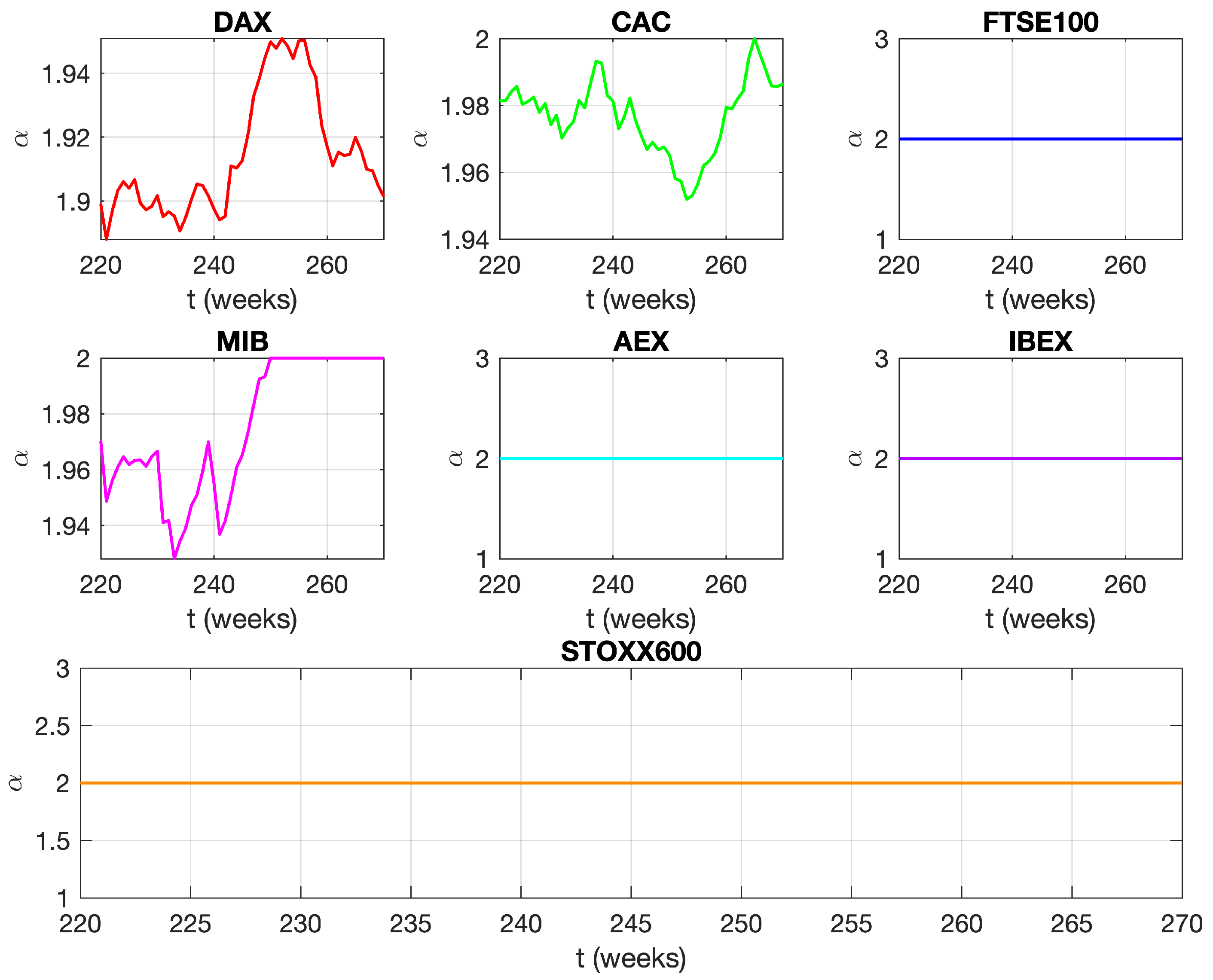
The model assumes that the noise term of the stochastic equation, Equation (3), takes steps from an α -Lévy stable distribution. For financial time series the value of α is frequently 2, and lesser values are discarded. Indeed, Figure 2, which displays the value of α with respect to time, makes it evident that the indices DAX and CAC always have α values below 2. In contrast, the value of α for the FTSE100, AEX, IBEX, and STOXX600 indexes is consistent with the value of 2. These results demonstrate that FTSE100, AEX, IBEX, and STOXX600 are processes that use steps from a Gaussian distribution, specifically a fractional Brownian motion (fBm), if H is constant over time, or a multifractional Brownian motion (mfBm), if H changes, with increments that correspond to a fractional Gaussian noise (fGn). Conversely, the DAX and CAC indexes use a non-Gaussian probability distribution to determine their steps, and an α -Lévy stable noise ( α -Lsn) determines their increments. Finally, for the first forecast points, the index MIB’s α value is less than two, and after that, it settles at two.
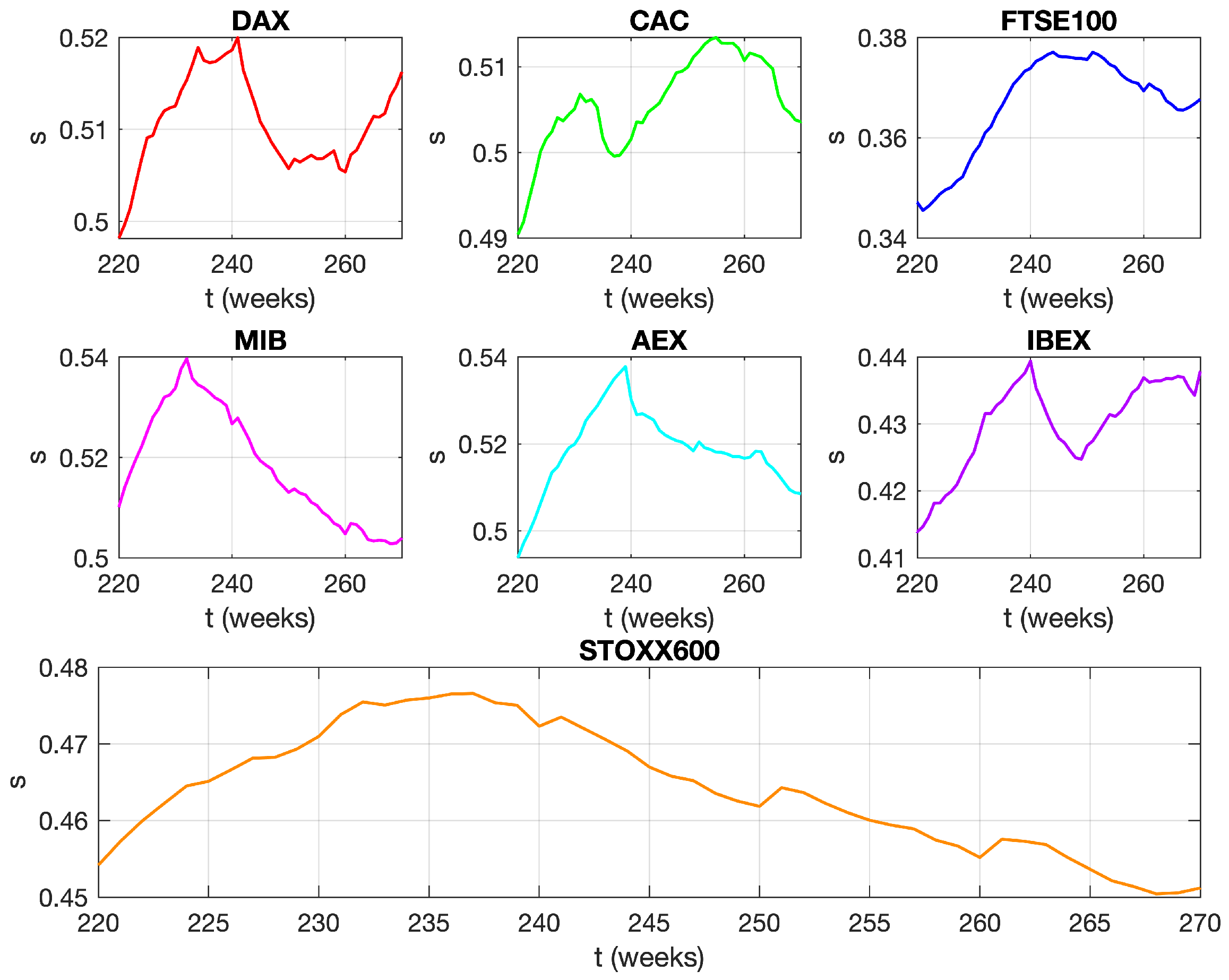
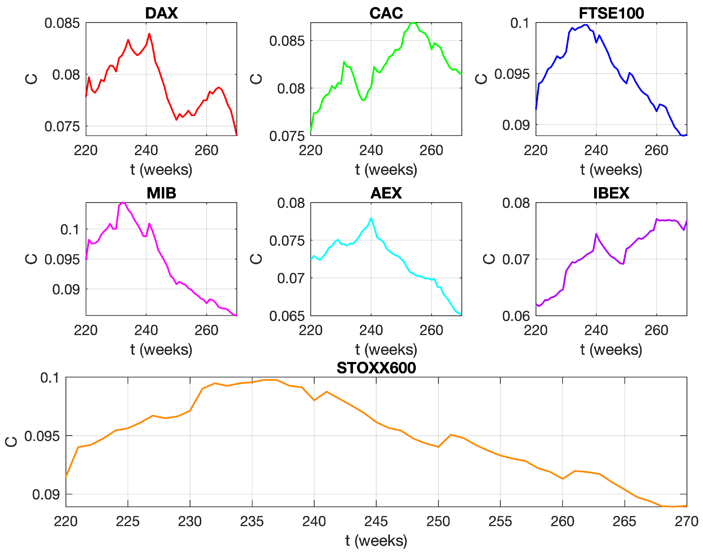
The time series displayed in Figure 1 are non-stationary and thus represent processes that are out of equilibrium. To prove that, we consider the increments of each one of them, which are then analyzed by GMM. Each analysis returns a Hurst exponent with a value of zero; results are not shown. Next, we consider the original time series whose thorough investigation based on the generalized moments method approach(GMM) [7,12,13,14,19,47] delivers the values of H, C, and α . Refer to Figure 3, Figure 4 and Figure 5, which show the scaling exponent (s), the mean intermittency parameter (C), and the Lévy stable index ( α ) versus time.
This study uses a minimal value of k equal to 0.8 N , although it can be even smaller. A process of length k is analyzed, and its length increases by 1 at each iteration. With N representing the entire length of each trajectory shown in Figure 1, the maximum value the index k can take is N 1 . Observe that even if smaller trajectories have been treated in the literature, the GMM requires a minimum of 100 points for a successful application [40].
From trading week to trading week, the value of the scaling exponent fluctuates; see Figure 3, and its value is directly connected to the type of stochastic process: 0.5 for white noise and coloured otherwise. Notice that there exist various types of white and coloured noises [5]. As it was mentioned, the scaling exponent satisfies the relation s = H 1 2 + 1 α , and thus, when α = 2 , the scaling exponent coincides with the Hurst exponent ( H = z ( q = 1 ) ). Unlike persistency ( s > 0.5 ), which shows the presence of temporal drifts, anti-persistency ( s < 0.5 ) shows a propensity for prices to return to their mean. Because their respective scaling exponents are consistently below the value of 0.5 during the course of the analysis window, the FTSE100, IBEX, and STOXX600 return to their average value (anti-persistent behavior). Instead, for DAX, CAC, MIB, and AEX, their scaling fluctuates in a very narrow range around or just above the value of 0.5, which points to an uncorrelated process (white noise). However, since the mean intermittency parameter is non-zero (see below), this uncorrelated process concerns the logarithm of the distribution and not the distribution itself. It is log-normal distributed when α = 2 , and log- α -Lévy stable when α < 2 .
The value of the mean of the intermittency parameter (C) approximately falls between 0.05 and 0.11, see Figure 4. Values of C constantly different than 0 point to a multifractal process, which, in conjunction with the values of the parameter α , classify the processes examined here as multifractal fractional Brownian motion (mfBm) [37] for FTSE100, AEX, IBEX, and STOXX600; as fractional Lévy-stable motion (fLsm) for DAX and CAC; and as fLsm that turns to mfBm for MIB. When shuffling input data, GMM analysis yields zero scaling exponents, indicating stationary processes. The latter underlines that multifractality originates from long-range correlations or, in other words, pattern formations that shuffling destroys.
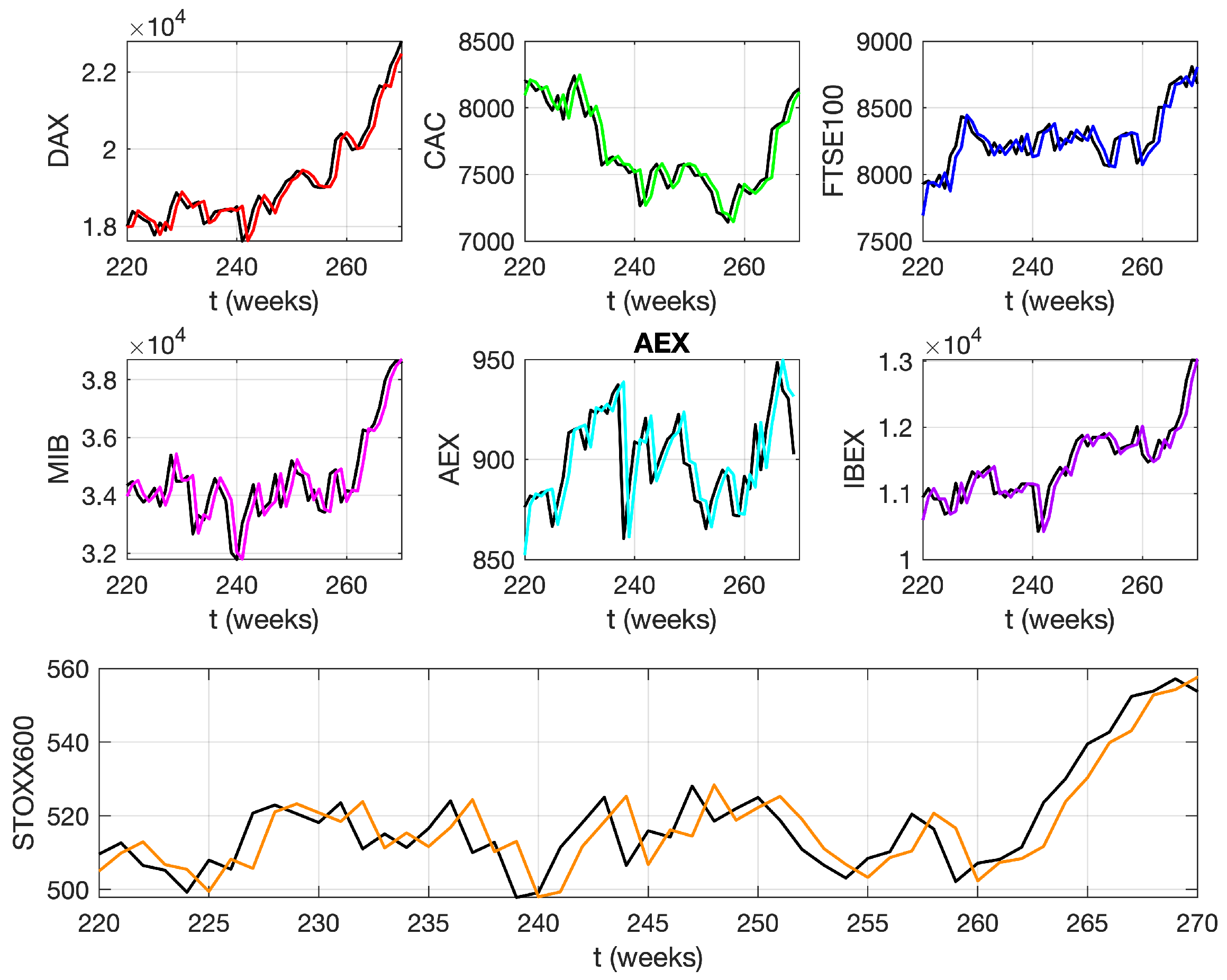
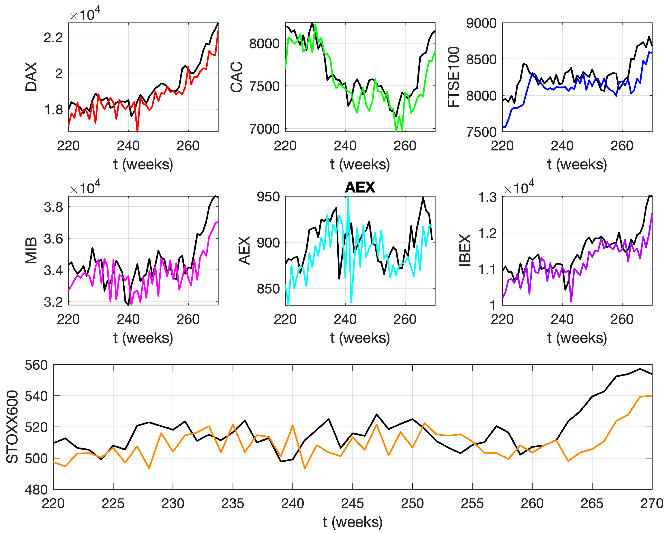
We utilize Equation (3) to forecast the data in Figure 1. At each iterative step, the values of α and H are used to create an α -Lévy stable motion, whose increments describe either a fractional Lévy stable noise or fractional Gaussian noise (fGn). For the creation of fractional Lévy stable noise sequences, we use Matlab’s built-in function STBL (Alpha stable distributions for MATLAB R2022b) [50]. This function takes four inputs: the value of α computed by GMM, the skewness parameter that is also available as the third central moment computed by GMM, the scale parameter also available as the second central moment, and the position parameter that is considered zero in all cases. The function returns an α -Lévy stable white noise that must be transformed to have the same properties as the original input data set. We first calculate the power spectrum, which is flat, and then multiply it by f β to produce the correct scale. Remember that β = 2 ( H 1 2 + 1 α ) + 1 . Next, applying the inverse Fourier transform, we end up with the sequence in the time domain [51,52]. For each iteration of length k, 1500 of such sequences are generated. The last members of them, indicated by the non-vanishing autocorrelation function, contribute to the value of the sequence at the point k+1. The mean of all forecasts for the point k+1 is then used in Equation (3). The forecasts are shown in Figure 5.
The recorded evidence is satisfactorily correlated with the forecasts. For some points, though, the trend between the predicted and actual values differs. The ability of the current model to forecast should be compared to some well-established models. An ARIMA-based forecast combined with Monte Carlo (MC) simulations is used [53]. The first k points of the input data shape the ’historical data’, and the time horizon for the forecast is one-step-ahead. Various ARIMA models have been fitted to ’historical data’, and the ARIMA(2,1,2) best performs based on both the Akaike information criterion (AIC) and the Bayesian information criterion (BIC), both of which have lower values at the same time. First ARIMA(2,1,2) is used to fit the data, then it makes a forecast for the time horizon, and finally, MC based on this forecast creates a number of paths whose mean at each point is the final forecast. For every forecast, 1500 simulations are performed. Matlab built-in functions have been used for the calculations [50], and the results are illustrated in Figure 6.
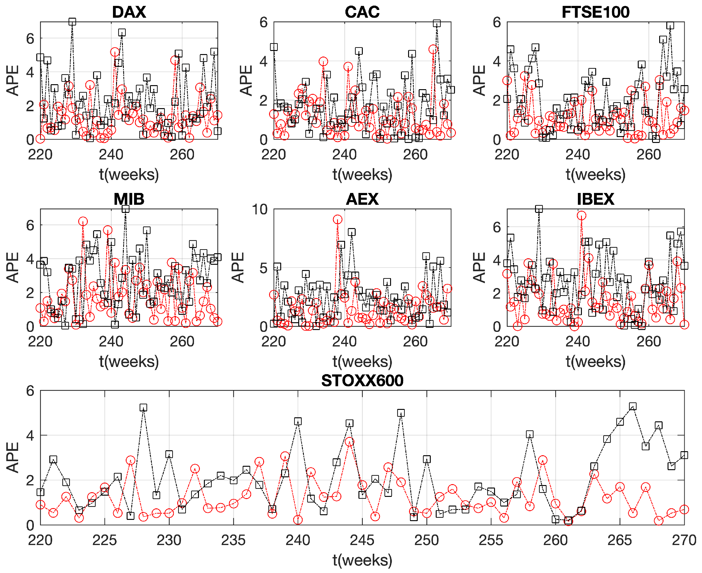
The ARIMA(2,1,2) based predictions combined with MC simulations correlate also well with the recorded values; see Figure 6. Comparing the outcomes of the two models, it is important to keep in mind that each forecast is based on historical data of varying lengths; therefore, the idea of the mean cannot be used. Rather, a metric that is not dependent on the actual values of the forecasts is needed. Such a metric is the absolute percentage error (APE), which is defined as A P E ( t ) = x ( t ) x f ( t ) x ( t ) where x ( t ) and x f ( t ) are the actual and the forecast values, respectively, at time t. Figure 7 displays the APE for both models.
Setting the value 5 for the APE to be the upper limit for an accurate forecasting model, we see that both functions well since few values for either model go above this threshold, see Figure 7. Forecasting based on the α -Lévy stable model returns values of APE that have an upper limit that does not exceed the value of 4, while forecasting based on the ARIMA(2,1,2) combined with MC simulation generally yields slightly higher values.
For every market examined in this work, are the predictions made by the two models equally accurate? The Diebold–Mariano (DM) test provides an answer to this question [54,55]. By setting as significant level the value of p = 0.05 , we run the DM test [56], where the first input corresponds to the forecasts of the present model, the second to the forecasts of ARIMA(2,1,2), and the third one equals one for the forecast horizon. The null hypothesis (both forecasts are equally good) is accepted if | D M | > 1.96 ; if not, it is rejected. For STOXX600/FTSE100/DAX/CAC/MIB/AEX/IBEX the test’s computed values are −3.63/−3.50/−3.21/−2.18/−3.35/−2.15/−3.93 and for none of them is the null hypothesis satisfied. Moreover, given that all computed values are negative, the forecasts of the present model (first input) perform better than the forecasts of the second one (ARIMA(2,1,2)): negative values indicate less average loss.
The forecasts of the present model and actual data patterns are consistent for most of the evidence that has been documented, and there is an acceptable link between the two. Thus, an α -Lévy stable noise, which describes the stochastic term of a forecasting process based on Equation (4), forecasts successfully in a time horizon of one-step-ahead even for small time series. The values of APE show how capable the model is.

4. Conclusions

In this work, we analyze and forecast several European market indices whose experimental evidence forms short time series with lengths shorter than 300 points, a five-year period from 2020 to 2025, and a sampling rate of 1 week. The forecasting is based on an iterative stochastic equation whose diffusive term for each temporal length is defined by a proper α -Lsm, the parameters of which are provided by the method of generalized moments(GMM). STOXX 600, FTSE100, AEX, and IBEX follow a distribution with α = 2 , as opposed to CAC and DAX, whose values are constantly lower than 2, while MIB partially follows a distribution with α = 2 . The values of the parameters H, C, and α classify the markets FTSE100, AEX, IBEX, STOXX600 and partially classify MIB as mfBm under the different windows of analysis. DAX, CAC, and partially MIB are classified as multifractal fractional α -Lévy stable motions. The process is anti-persistent for FTSE100, IBEX, and STOXX600, and the other markets reflect processes whose values are uncorrelated and drawn from a log-normal or log-Lévy distribution. The model was tested against the forecasts of a properly chosen ARIMA model combined with MC simulations. The APE for each forecast and for each model has been calculated, showing that both work well with a value of 4 to serve as an upper limit of APE for the majority of the forecasts for the suggested model. In addition, the Diebold–Mariano test showed that forecasting based on the α -Lévy stable model performs better than the corresponding one based on ARIMA. The small values of APE for all forecasts and for all examined markets show that the suggested model works well even if small time series are considered.

Funding

This research received no external funding.

Institutional Review Board Statement

Not applicable.

Informed Consent Statement

Not applicable.

Data Availability Statement

Publicly available datasets were analyzed in this study. This data can be found here: https://www.statista.com/.

Conflicts of Interest

The author declares no conflicts of interest.

Abbreviations

The following abbreviations are used in this manuscript:
fBmfractional Brownian motion
fGnfractional Gaussian noise
mfBmmultifractional fractional Brownian motion
fLsmfractional Lévy stable motion
fLsnfractional Lévy stable noise
ARIMAAutoregressive Integrated Moving Average
MCMonte Carlo
DMDiebold–Mariano test

References

  1. Börner, K.; Rouse, W.B.; Trunfio, P.; Stanley, H.E. Forecasting innovations in science, technology, and education. Proc. Natl. Acad. Sci. USA 2018, 115, 12573–12581. [Google Scholar] [CrossRef]
  2. Baker, G.L.; Gollub, J.P. Chaotic Dynamics an Introduction, 2nd ed.; Oxford University Press: Oxford, UK, 1996. [Google Scholar]
  3. Prado, T.L.; Boaretto, B.R.; Corso, G.; dos Santos, L.G.Z.; Kurths, J.; Lopes, S.R. A direct method to detect deterministic and stochastic properties of data. New J. Pjys. 2022, 24, 033027. [Google Scholar] [CrossRef]
  4. Hänggi, P.; Thomas, H. Stochastic processes: Time evolution, symmetries and linear response. Phys. Rep. 1982, 88, 207–319. [Google Scholar] [CrossRef]
  5. Bakalis, E.; Lugli, F.; Zerbetto, F. Daughter Coloured Noises: The Legacy of Their Mother White Noises Drawn from Different Probability Distributions. Fractal Fract. 2023, 7, 600. [Google Scholar] [CrossRef]
  6. Eke, A.; Herman, P.; Bassingthwaighte, J.; Raymond, G.; Percival, D.; Cannon, M.; Balla, I.; Ikrényi, C. Physiological time series: Distinguishing fractal noises from motions. Pflugers Arch. 2000, 439, 403–415. [Google Scholar] [CrossRef] [PubMed]
  7. Bakalis, E.; Gavriil, V.; Cefalas, A.-C.; Kollia, Z.; Zerbetto, F.; Sarantopoulou, E. Viscoelasticity and Noise Properties Reveal the Formation of Biomemory in Cells. J. Phys. Chem. B 2021, 125, 10883–10892. [Google Scholar] [CrossRef]
  8. Hurst, H.E. Long term storage capacity of reservoirs. Trans. Am. Soc. Eng. 1951, 116, 770–799. [Google Scholar] [CrossRef]
  9. Mandelbrot, B.B.; Wallis, J.R. Robustness of the rescaled range R/S in the measurement of noncyclic long run Statistical dependence. Water Resour. Res. 1969, 5, 967–988. [Google Scholar] [CrossRef]
  10. Di Matteo, T. Multi-scaling in finance. Quant. Financ. 2007, 7, 21–36. [Google Scholar] [CrossRef]
  11. Barabási, A.-L.; Viscek, T. Multifractality of self-affine fractals. Phys. Rev. A 1991, 44, 2730. [Google Scholar] [CrossRef]
  12. Bakalis, E.; Höfinger, S.; Venturini, A.; Zerbetto, F. Crossover of two power laws in the anomalous diffusion of a two lipid membrane. J. Chem. Phys. 2015, 142, 215102. [Google Scholar] [CrossRef] [PubMed]
  13. Sändig, N.; Bakalis, E.; Zerbetto, F. Stochastic analysis of movements on surfaces: The case of C60 on Au(1 1 1). Chem. Phys. Lett. 2015, 633, 163–168. [Google Scholar] [CrossRef]
  14. Bakalis, E.; Mertzimekis, T.J.; Nomikou, P.; Zerbetto, F. Breathing modes of Kolumbo submarine volcano (Santorini, Greece). Sci. Rep. 2017, 7, 46515. [Google Scholar] [CrossRef]
  15. Caccia, D.C.; Percival, D.; Cannon, M.J.; Raymond, G.; Bassingthwaighte, J.B. Analyzing exact fractal time series: Evaluating dispersional analysis and rescaled range methods. Physica A 1997, 246, 609–632. [Google Scholar] [CrossRef] [PubMed]
  16. Eke, A.; Herman, P.; Kocsis, L.; Kozak, L.R. Fractal characterization of complexity in temporal physiological signals. Physiol. Meas. 2002, 23, R1–R38. [Google Scholar] [CrossRef]
  17. Peng, C.-K.; Buldyrev, S.V.; Havlin, S.; Simons, M.; Stanley, H.E.; Goldberger, A.L. Mosaic organization of DNA nucleotides. Phys. Rev. E 1994, 49, 685–1689. [Google Scholar] [CrossRef]
  18. Kantelhardt, J.W.; Zschiegner, S.A.; Koscielny-Bunde, E.; Havlin, S.; Bunde, A.; Stanley, H.E. Multifractal detrended fluctuation analysis of nonstationary time series. Physica A 2002, 316, 87–114. [Google Scholar] [CrossRef]
  19. Bakalis, E.; Ferraro, A.; Gavriil, V.; Pepe, F.; Kollia, Z.; Cefalas, A.-C.; Malapelle, U.; Sarantopoulou, E.; Troncone, G.; Zerbetto, F. Universal Markers Unveil Metastatic Cancerous Cross-Sections at Nanoscale. Cancers 2022, 14, 3728. [Google Scholar] [CrossRef]
  20. Gómez-Águila, A.; Trinidad-Segovia, J.E.; Sánchez-Granero, M.A. Improvement in Hurst exponent estimation and its application to financial markets. Financ. Innov. 2022, 8, 86. [Google Scholar] [CrossRef]
  21. Taqqu, M.S.; Teverovsky, V.; Willinger, W. Estimators for long-range dependence: An empirical study. Fractals 1995, 3, 785–798. [Google Scholar] [CrossRef]
  22. Barunik, J.; Kristoufek, L. On Hurst exponent estimation under heavy-tailed distributions. Physica A 2010, 389, 3844–3855. [Google Scholar] [CrossRef]
  23. Black, F.; Scholes, M. The pricing of options and corporate liabilities. J. Political Econ. 1973, 81, 637–654. [Google Scholar] [CrossRef]
  24. Plerou, V.; Gopikrishnan, P.; Rosenow, B.; Amaral, L.A.N.; Stanley, H.E. Econophysics: Financial time series from a statistical physics point of view. Physica A 2000, 279, 443–456. [Google Scholar] [CrossRef]
  25. Mandelbrot, B. The Variation of Certain Speculative Prices. J. Bus. 1963, 36, 394–419. [Google Scholar] [CrossRef]
  26. Mantegna, R.; Stanley, H.E. Scaling behaviour in the dynamics of an economic index. Nature 1995, 376, 46–49. [Google Scholar] [CrossRef]
  27. Bouchaud, J.P.; Potters, M.; Meyer, M. Apparent multifractality in financial time series. Eur. Phys. J. B 2000, 13, 595–599. [Google Scholar] [CrossRef]
  28. Scalas, E. Scaling in the market of futures. Physica A 1998, 253, 394–402. [Google Scholar] [CrossRef]
  29. Calvet, L.; Fisher, A. Multifractality in Asset Returns: Theory and Evidence. Rev. Econ. Stat. 2002, 84, 381–406. [Google Scholar] [CrossRef]
  30. Ruipeng, L.; Di Matteo, T.; Lux, T. Multifractality and long-range dependence of asset returns: The scaling behaviour of the Markov-switching multifractal model with lognormal volatility components. Adv. Complex Syst. 2008, 11, 669–684. [Google Scholar] [CrossRef]
  31. Mantegna, R.N. Lévy walks and enhanced diffusion in Milan stock exchange. Physica A 1991, 179, 232–242. [Google Scholar] [CrossRef]
  32. Mandelbrot, B.B.; Van Ness, J.W. Fractional brownian motions, fractional noises and applications. SIAM Rev. 1968, 10, 422–437. [Google Scholar] [CrossRef]
  33. Samorodnitsky, G.; Taqqu, M. Stable Non-Gaussian Random Processes: Stochastic Models with Infinte Variance, 1st ed.; Chapman and Hall: New York, NY, USA, 1994. [Google Scholar]
  34. Fama, E.F.; Roll, R. Some properties of symmetric stable distributions. Am. Stat. Assoc. J. 1968, 63, 817–836. [Google Scholar] [CrossRef]
  35. Kogon, S.M.; Manolakis, G. Signal modeling with self-similar α/-stable processes: The fractional Levy stable motion model. IEEE Trans. Signal Process. 1996, 44, 1006–1010. [Google Scholar] [CrossRef]
  36. Samorodnitsky, G.; Taqqu, M. Linear models with long-range dependence and with finite and infinite variance. In New Directions in Time Series Analysis. The IMA Volumes in Mathematics and Its Applications, 1st ed.; Brillinger, D., Caines, P., Geweke, J., Parzen, E., Rosenblatt, M., Taqqu, M.S., Eds.; Springer: New York, NY, USA, 1993; pp. 325–340. [Google Scholar]
  37. Song, W.; Cattani, C.; Chi, C.-H. Multifractional Brownian motion and quantum-behaved particle swarm optimization for short term power load forecasting: An integrated approach. Energy 2020, 194, 116847. [Google Scholar] [CrossRef]
  38. Liu, H.; Song, W.; Li, M.; Kudreyko, A.; Zio, E. Fractional Lévy stable motion: Finite difference iterative forecasting model. Chaos 2020, 133, 109632. [Google Scholar] [CrossRef]
  39. Bakalis, E.; Zerbetto, F. Iterative Forecasting of Financial Time Series: The Greek Stock Market from 2019 to 2024. Entropy 2025, 27, 497. [Google Scholar] [CrossRef]
  40. Bakalis, E.; Parent, L.R.; Vratsanos, M.; Chiwoo, P.; Gianneschi, N.C.; Zerbetto, F. Complex Nanoparticle Diffusional Motion in Liquid-Cell Transmission Electron Microscopy. J. Phys. Chem. C 2020, 124, 14881. [Google Scholar] [CrossRef]
  41. Schertzer, D.; Lovejoy, S. Physical modeling and Analysis of Rain and Clouds by Anisotropic Scaling of Multiplicative Processes. J. Geophys. Res. 1987, 92, 9693–9714. [Google Scholar] [CrossRef]
  42. Laskin, N.; Lambadaris, I.; Harmantzis, F.C.; Devetsikiotis, M. Fractional Lévy motion and its application to network traffic modeling. Comput. Netw. 2002, 40, 363–375. [Google Scholar] [CrossRef]
  43. Mandelbrot, B.B. The Fractal Geometry of Nature, 1st ed.; W. H. Freeman & Company: New York, NY, USA, 2008; p. 480. [Google Scholar]
  44. Lyra, M.L.; Tsallis, C. Nonextensivity and multifractality in low-dimensional dissipative systems. Phys. Rev. Lett. 1998, 80, 53–56. [Google Scholar] [CrossRef]
  45. Jiang, Z.-Q.; Xie, W.-J.; Zhou, W.-X.; Sornette, D. Multifractal analysis of financial markets: A review. Rep. Prog. Phys. 2019, 82, 125901. [Google Scholar] [CrossRef] [PubMed]
  46. Kolmogorov, A.N. A refinement of previous hypotheses concerning the local structure of turbulence in a viscous incompressible fluid at high Reynolds number. J. Fluid Mech. 1962, 13, 82–85. [Google Scholar] [CrossRef]
  47. Bakalis, E.; Fujie, H.; Zerbetto, F.; Tanaka, Y. Multifractal structure of microscopic eye–head coordination. Physica A 2018, 512, 945–953. [Google Scholar] [CrossRef]
  48. Janicki, A.; Weron, A. Can One See α-Stable Variables and Processes? Stat. Sci. 1994, 9, 109–126. [Google Scholar] [CrossRef]
  49. Available online: https://www.statista.com/search/?q=weekly+indexes+2020+-+2025+europe&Search=&p=1 (accessed on 21 July 2025).
  50. The MathWorks Inc. MATLAB, Version: 9.13.0 (R2022b); The MathWorks Inc.: Natick, MA, USA, 2022.
  51. Kasdin, N. Discrete simulation of colored noise and stochastic processes and 1/fα power law noise generation. Proc. IEEE 1995, 83, 802–827. [Google Scholar] [CrossRef]
  52. Zhivomirov, H. Pink, Red, Blue and Violet Noise Generation with Matlab Implementation, Version 1.6. Available online: https://www.mathworks.com/matlabcentral/fileexchange/42919-pink-red-blue-and-violet-noise-generation-with-matlab-implementation (accessed on 15 November 2017).
  53. Chen, Z. Asset Allocation Strategy with Monte-Carlo Simulation for Forecasting Stock Price by ARIMA Model. In Proceedings of the IC4E ’22: Proceedings of the 2022 13th International Conference on E-Education, E-Business, E-Management, and E-Learning, Tokyo, Japan, 14–17 January 2022; pp. 481–485. [Google Scholar] [CrossRef]
  54. Diebold, F.X.; Mariano, R.S. Comparing Predictive Accuracy. J. Bus. Econ. Stat. 1995, 13, 253–263. [Google Scholar] [CrossRef]
  55. Harvey, D.; Leybourne, S.; Newbold, P. Testing the equality of prediction mean squared errors. Int. J. Forecast. 1997, 13, 281–291. [Google Scholar] [CrossRef]
  56. Ibisevic, S. Diebold-Mariano Test Statistic. MATLAB Central File Exchange. Available online: https://ch.mathworks.com/matlabcentral/fileexchange/33979-diebold-mariano-test-statistic (accessed on 15 October 2025).
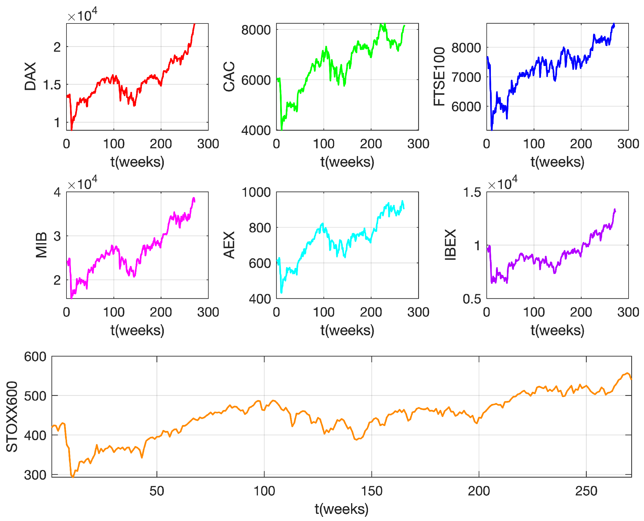
Figure 1. Each one of the panels displays a different index (DAX in red, CAC in green, FTSE100 in blue, MIB in magenta, AEX in cyan, IBEX in purple, and STOXX600 in orange) over a five-year period, from 2020 to 2025. Consecutive events have a distance of one week.
Applsci 15 11580 g001
Figure 2. α parameters in time for several indices. The computed values are shown for historical data with lengths that go from 0.8 N to N 1 , with N being the total length.
Applsci 15 11580 g002
Figure 3. Scaling exponent between a minimum of 220 weeks and a maximum of 270 weeks. With every new trade week, the length of time that data is accumulated increases by one.
Applsci 15 11580 g003
Figure 4. The mean intermittency parameter C for each market. The values are between a minimum of 220 weeks and a maximum of 270 weeks.
Applsci 15 11580 g004
Figure 5. In black displays the evolution of each market index based on a weekly sampling rate over a constrained time frame of five years (2020–2025). The forecasting values at the same time frame are represented by the coloured curves.
Applsci 15 11580 g005
Figure 6. It shows the same information as Figure 5 but for forecasts based on ARIMA(2,1,2). Again, black for the evolution of each market and coloured curves for the forecasts.
Applsci 15 11580 g006
Figure 7. Absolute percentage error (APE) for one-step-ahead forecast. Red for the present model and black for ARIMA(2,1,2).
Applsci 15 11580 g007
Disclaimer/Publisher’s Note: The statements, opinions and data contained in all publications are solely those of the individual author(s) and contributor(s) and not of MDPI and/or the editor(s). MDPI and/or the editor(s) disclaim responsibility for any injury to people or property resulting from any ideas, methods, instructions or products referred to in the content.