Article

Common Calibration of Solar Radiation and Net Longwave Radiation Is the Key to Accurately Estimating Reference Crop Evapotranspiration over the Tibetan Plateau

by
Jiandong Liu
1,
Guangsheng Zhou
1,*,
Jun Du
2,*,
Mingxing Li
3,
Yanling Song
1,
Shang Chen
4 and
Yuhe Ji
1
1
State Key Laboratory of Severe Weather, Institute of Agro-Meteorology, Chinese Academy of Meteorological Sciences, China Meteorological Administration, Beijing 100081, China
2
Tibet Climate Center, Tibet Autonomous Meteorological Administration, Lhasa 850001, China
3
Key Laboratory of Regional Climate-Environment for Temperate East Asia, Institute of Atmospheric Physics, Chinese Academy of Sciences, Beijing 100029, China
4
Jiangsu Key Laboratory of Agricultural Meteorology, Nanjing University of Information Science and Technology, Nangjing 210044, China
*
Authors to whom correspondence should be addressed.
Appl. Sci. 2025, 15(23), 12449; https://doi.org/10.3390/app152312449
Submission received: 4 November 2025 / Revised: 21 November 2025 / Accepted: 22 November 2025 / Published: 24 November 2025
(This article belongs to the Section Earth Sciences)

Abstract

Reference crop evapotranspiration (ET0) is crucial for water management. Although the FAO56-PM method is widely used to estimate ET0, its input variables of solar radiation (Rs) and net longwave radiation (Rnl) are not readily available. Currently, mere calibration of the formula for Rs is assumed to be effective in improving FAO56-PM’s performance. To test this hypothesis, all input variables for FAO56-PM were measured in Lhasa, Linzhi, and Bange over the Tibetan Plateau (TP) to assess how different calculation methods affect ET0 estimates. Compared to the original FAO56-PM, calibration of both Rs and Rnl formulas yielded the best model performance. Mere calibration of the formula for Rnl notably improved ET0 estimation accuracy, while mere calibration of the formula for Rs reduced its accuracy. The general calibration model was slightly less effective than calibration of both Rs and Rnl formulas but obviously outperformed the original FAO56-PM. This model showed that ET0 increased from east to west, ranging from 569.4 mm/year to 1118.5 mm/year. Trend analysis indicated rapid increases in ET0 in the eastern region and significant decreases in the western region of the TP over recent decades. The findings are useful for the regional application of FAO56-PM to achieve sustainable development in Tibet.

1. Introduction

Evapotranspiration (ET) plays a crucial role in the hydrological cycle and water balance [1,2,3]. Accurate ET estimation is vital, serving as a key element in hydrological [4,5,6] and crop growth models [7,8,9]. Additionally, precise ET data is essential for developing optimal strategies in agricultural water management [10,11,12], and it is particularly important for crafting policies that promote sustainable agriculture in water-scarce areas such as the Tibetan Plateau [13].
ET can be measured directly using instruments like lysimeters or eddy covariance measurements [14,15], but these methods are laborious, time-consuming, and costly [16]. Currently, ET is typically estimated using the two-step approach recommended by the Food and Agriculture Organization (FAO). This method calculates ET as the product of reference crop evapotranspiration (ET0) and the crop coefficient [13,17,18]. Therefore, accurate estimation of ET0 is important for reliable ET calculations.
ET0 is defined as the evapotranspiration rate from a surface of green grass with a uniform height of 8–15 cm. The grass is assumed to be actively growing, fully shading the ground, and free from water stress [19]. Numerous models have been developed to estimate ET0 [20], which can be categorized into four main types [21]: combination-based models [17,22,23], radiation-based models [24,25,26], temperature-based models [27,28,29], and aerodynamic models [30,31,32]. Among these, the FAO-56 Penman–Monteith model [17] (FAO56-PM for short) is considered the most reliable for ET0 estimation. It is often used as the standard for evaluating other models [21,33,34], and is applied globally [35,36,37].
Application of the FAO-56 PM method is often limited by its required input variables, which include maximum and minimum temperatures, water vapor pressure, wind speed, and radiation-related variables [17]. Among these, maximum and minimum temperatures, water vapor pressure, and wind speed are readily available at most weather stations (for example, all 2400 weather stations in China routinely measure these variables). However, radiation-related variables such as solar radiation (Rs) and net longwave radiation (Rnl) are measured at only a very few stations (for instance, Rs is measured at approximately 140 stations in China, while Rnl is only recorded in specific radiation observation experiments). To address this, the Angstrom formula is recommended for estimating Rs. The Allen formula, based on the Stefan–Boltzmann law, is used for estimating Rnl in the FAO-56 PM method [17].
The introduction of these two formulas has caused confusion regarding the standard ET0 by FAO-56 PM. Some scientists believe that the standard ET0 should be calculated strictly using the recommended formulas and default coefficients [21,33,35]. Conversely, many scientists believe that Rs, estimated using the recommended Angstrom formula and default coefficients, may not be reliable. They suggest that Rs should first be estimated using a calibrated Angstrom formula or other methods, and then the standard ET0 by FAO-56 PM can be obtained using the estimated Rs. In this process, Rnl should be calculated strictly according to the recommended Allen formula and default coefficients [38,39,40].
However, Allen et al. [17] stated that “where measurements of incoming and outgoing short and longwave radiation during bright sunny and overcast hours are available, calibration of the coefficients in Equation (39) can be carried out” ([17], p. 52. Here, Equation (39) refers to the formula for net longwave radiation). This statement indicates clearly that all input variables, including both Rs and Rnl, should be measurements rather than estimates. In other words, the standard ET0 by FAO-56 PM refers to the ET0 calculated with all measured input variables, including measured Rs and Rnl. Using the FAO-56 PM with the recommended formulas and default coefficients should only be considered as a last resort when no measurements are available, and the results cannot be regarded as the standard ET0 by FAO-56 PM. The formulas for both Rs and Rnl should be calibrated simultaneously whenever measurements are available [17].
Based on the arguments above, errors in ET0 estimation will arise from both Rs and Rnl, if no calibration of the recommended formulas is performed. It is generally assumed that calibrating Rs would partly reduce these errors, a topic that has recently gained attention from researchers [41,42,43,44]. However, Rnl can also play an important role in energy balance in certain regions [45,46,47], especially in the alpine regions like the Tibetan Plateau, where high Rnl was identified [48]. In such climates, it is reasonable to hypothesize that errors in ET0 estimation might decrease if the errors from the recommended formulas have the same sign for both Rs and Rnl to result in offsetting effects (i.e., both are overestimated or underestimated simultaneously). In this situation, studies focusing solely on calibrating Rs may not reduce, but rather increase, the errors in ET0 estimation. Simultaneous calibration of both Rs and Rnl is the only effective method for accurate ET0 estimation. However, up to now, few studies have addressed the simultaneous calibration of both Rs and Rnl, particularly in alpine regions like the Tibetan Plateau.
The Tibetan Plateau (TP), located in southwestern China, is the largest plateau in the country and the highest globally. Highland barley serves as the staple food for the Tibetan population, yet its cultivation is constrained by local water conditions [49]. Accurate data on evapotranspiration is crucial for the local government to develop effective irrigation plans. Despite having around 40 weather stations scattered over the TP, routine measurements of Rs are only conducted at Lhasa and Linzhi stations, while Rnl is not routinely measured at any station. However, Rnl has been recorded in Lhasa and Linzhi during experiments in recent years, and measurements of both Rs and Rnl were taken from 2014 to 2015 at Bange during the Third Scientific Expedition over the Tibetan Plateau.
In this study, for the first time, supported by complete data required for FAO56-PM, including measurements of both Rs and Rnl, we calibrated the recommended formulas for Rs and Rnl in FAO56-PM over the TP, aiming to (1) analyze errors in ET0 arising from the recommended formulas for Rs and Rnl; (2) assess the significance of mere calibration of Rs for ET0 estimation; and (3) comprehensively calibrate both Rs and Rnl for accurate ET0 estimation over the TP. Ultimately, a general model was developed for regional application of FAO56-PM, which was used to calculate the spatial distribution and temporal trend of ET0, in order to support sustainable agricultural development in this region.

2. Materials and Methods

2.1. Description of the Study Region

Situated in southwestern China, the TP is the world’s highest plateau, known for its complex terrain [50]. Approximately 40 weather stations are sparsely distributed across the region (Figure 1). These stations routinely measure basic meteorological variables such as sunshine duration, maximum and minimum temperatures, vapor pressure, and wind speed on a daily basis. Radiation-related variables, including both Rs and Rnl, are measured only during specific experiments or scientific expeditions at three stations: Lhasa, Linzhi, and Bange. The comprehensive data from these three stations were used for the calibration of FAO56-PM. The detailed information on the experimental sites and the weather stations is provided in Table 1.

2.2. Data Collection

2.2.1. Data on Basic Meteorological Variables

The basic meteorological variables, such as sunshine duration, maximum and minimum temperatures, vapor pressure, and wind speed, have been recorded daily at all weather stations in China. These data were compiled by the National Meteorological Information Center (NMIC), a division of the China Meteorological Administration (CMA). NMIC has developed the Tianqin platform, featuring a stringent data quality control system to maintain measurement accuracy. For this study, NMIC provided daily meteorological data from 1991 to 2020. The abnormal records accounted for approximately 0.75%, and were removed from the data sets in this study.

2.2.2. Data on Radiation-Related Variables

Daily Rs has been measured routinely at Lhasa and Linzhi since 1961. Rnl has been measured at Lhasa from 20 October 1993 to 31 December 2020, and at Linzhi from 1 September 2015 to 31 December 2020. Both Rs and Rnl were measured simultaneously at Bange from 1 August 2014 to 31 July 2015, during the Third Scientific Expedition over the Tibetan Plateau (TSETP).

2.2.3. Datasets Used for This Study

Two datasets were created for the comprehensive calibration and regional application of FAO56-PM. For comprehensive calibration, the data from Rnl measurements for Lhasa, Linzhi, and Bange were used. These measurements, along with the corresponding Rs and basic meteorological variables, were combined into a complete dataset for FAO56-PM comprehensive calibration. The coefficients were calibrated using data on odd-numbered days in this dataset. For regional application, basic meteorological variables from 1991 to 2020 were compiled into a dataset for all stations across the TP.

2.3. Description of FAO56-PM

The widely used FAO56-PM is expressed as [17]:
E T 0 = 0.408 R n G + ( 900 γ u 2 ( e s e a ) / T + 273 ) + γ ( 1 + 0.34 u 2 )
where ET0 represents the reference crop evapotranspiration (mm d−1); Δ is the slope of saturated vapor pressure-temperature curve (kPa °C−1); Rn is the net radiation (MJ m−2 d−1); G is the soil heat flux (MJ m−2 d−1); es and ea are the saturated and actual vapor pressure (kPa), respectively; γ is the psychrometric constant (kPa °C−1); T is mean air temperature (°C); u2 is wind speed at 2 m height (m s−1). For standardization, Allen et al. [17] defined T as the mean value of the daily maximum (Tmax) and minimum temperature (Tmin), rather than the average of the hourly temperature measurements.
T = T m a x + T m i n 2
The slope of the saturated vapor pressure-temperature curve Δ can be expressed as:
= 2504 exp 17.27 T / ( T + 237.3 ) T + 237.3 2
At the daily scale, the soil heat flux G can be neglected [17], so G = 0 in the Equation (1). The psychrometric constant γ is provided by:
γ = 0.665 × 10 3 p
where p is atmospheric pressure (kPa), calculated as follows [17]:
p = 101.3 293 0.0065 H 293 5.26
where H is the altitude (m) of the study site. Wind speed at 2 m (u2) can be calculated from the wind speed measured at a height of z m (uz) using the following equation:
u 2 = 4.87 l n ( 67.8 z 5.42 ) u z
The saturated vapor pressure es is the average of es (Tmax) and es (Tmin), calculated as:
e s t = 0.6108 e x p 17.27 t t + 237.3
where t denotes either Tmax or Tmin.
For most weather stations in China, all input variables except Rn are readily available for calculating ET0. The net radiation Rn is given by:
R n = 1 α × R s R n l
where Rn, Rs and Rnl represent net radiation, solar radiation (or downward shortwave radiation), and net longwave radiation, respectively. The coefficient α denotes albedo, and Allen et al. [17] set α to 0.23 for the reference crop.
If both Rs and Rnl are available, the standard ET0 can be calculated directly using FAO56-PM. However, obtaining Rs and Rln, particularly Rnl, is often difficult at most weather stations. Therefore, various methods exist to obtain Rs and Rnl, leading to different calculation methods for FAO56-PM as follows.

2.4. Calculation Methods

2.4.1. AllenM Method

If the input variables for both Rs and Rnl are measurements, the ET0 calculated using the FAO56-PM method is based on all measured input variables. In this case, the calculated ET0 is referred to as the standard value for FAO56-PM, and this method is defined as AllenM.

2.4.2. AllenO Method

If the measurements of both Rs and Rnl are not available, Allen et al. [17] recommended two empirical formulas for estimating Rs and Rnl. Rs is typically estimated using the Angstrom formula (Hereafter referred to as Fs):
R s R 0 = a + b × S S 0
where R0 represents extraterrestrial radiation, S is actual sunshine hours, and S0 is potential sunshine hours. In the absence of measured data for calibration, Allen et al. [17] suggested default values of 0.250 for coefficient a and 0.500 for coefficient b, respectively. The FAO56-PM model for calculating net longwave radiation is formulated as follows (Hereafter referred to as Fnl):
R n l = σ T m a x , k 4 + T m i n , k 4 2 c d e a e R s R s 0 f
where σ represents the Stefan–Boltzmann constant (4.895 × 10⁻⁶ MJ m−2 d−1 K−4); Tmax,k and Tmin,k denote the absolute maximum and minimum temperature in Kelvin, respectively. Rs stands for the solar radiation, while Rs0 indicates the calculated clear-sky solar radiation, typically derived from the Angstrom model under full sunshine conditions, where S = S0. The coefficients 0.34, 0.14, 1.35 and 0.35 are the default values for the coefficients of c, d, e and f, respectively, as recommended by Allen et al. [17]. This method is actually the original FAO56-PM, which is defined as AllenO.

2.4.3. AllenS Method

Considering the reliability of Rs, some scientists have focused on calibrating Fs in an effort to improve the accuracy of the FAO56-PM model. Mere calibration of Fs is defined as AllenS.

2.4.4. AllenL Method

In contrast to AllenS, mere calibration of Fnl without calibration of Fs is defined as AllenL.

2.4.5. AllenC Method

In contrast to AllenS and AllenL, comprehensive calibration of both Fs and Fnl is defined as AllenC.

2.4.6. AllenR Method

The calibrated coefficients for Fs and Fnl are site-specific, necessitating local calibration using measurements of both Rs and Rnl. This requirement makes it challenging, if not impossible, to apply AllenC on a regional scale. So, we developed a general method allows for the easy derivation of coefficients using geographic or basic meteorological parameters, facilitating its regional application over the TP.
Based on our previous study on estimating regional distribution of solar radiation over the TP [51], the coefficients for Fs over the TP can be calculated from the following functions.
a + b = 0.106 × ln H 0.060
b = 0.373 × 1 μ + 0.483
where µ is the average daily water vapor pressure (hPa). Based on all measured Rnl at Lhasa, Linzhi and Bange, a set of coefficients for Fnl can be obtained by calibrating Fnl against these measurements. This method can be easily applied at a regional scale and is referred to as AllenR.

2.5. Model Evaluation

The performance of these models was evaluated using root mean square error (RMSE), which measures random error; mean absolute percentage error (MAPE), which measures the error relative to the standard value; mean bias error (MBE), which measures systematic error; and coefficient of determination (R2), which measures the model fitting effect [52].
R M S E = 1 n i = 1 n ( C i M i ) 2
M A P E = 1 n i = 1 n C i M i M i × 100 %
M B E = 1 n i = 1 n ( C i M i )
  R 2 = i = 1 n M i M ¯ C i C ¯ 2 i = 1 n M i M ¯ 2 i = 1 n C i C ¯ 2
where Mi is the measured value; Ci is the calculated value; M ¯ and C ¯ are the average of the measured and calculated values, respectively, and n is the total sample number.

3. Results

3.1. Errors in Estimated ET0 Resulting from Recommended Fs and Fnl

First, the standard ET0 was calculated under the AllenM method, i.e., all of the input variables were measurements. Errors in the estimated ET0, arising from recommended Fs (or Fnl), were identified by replacing the measured Rs (or Rnl) with the values calculated using the recommended Fs (or Fnl).

3.1.1. Errors in Estimated ET0 Resulting from Recommended Fs

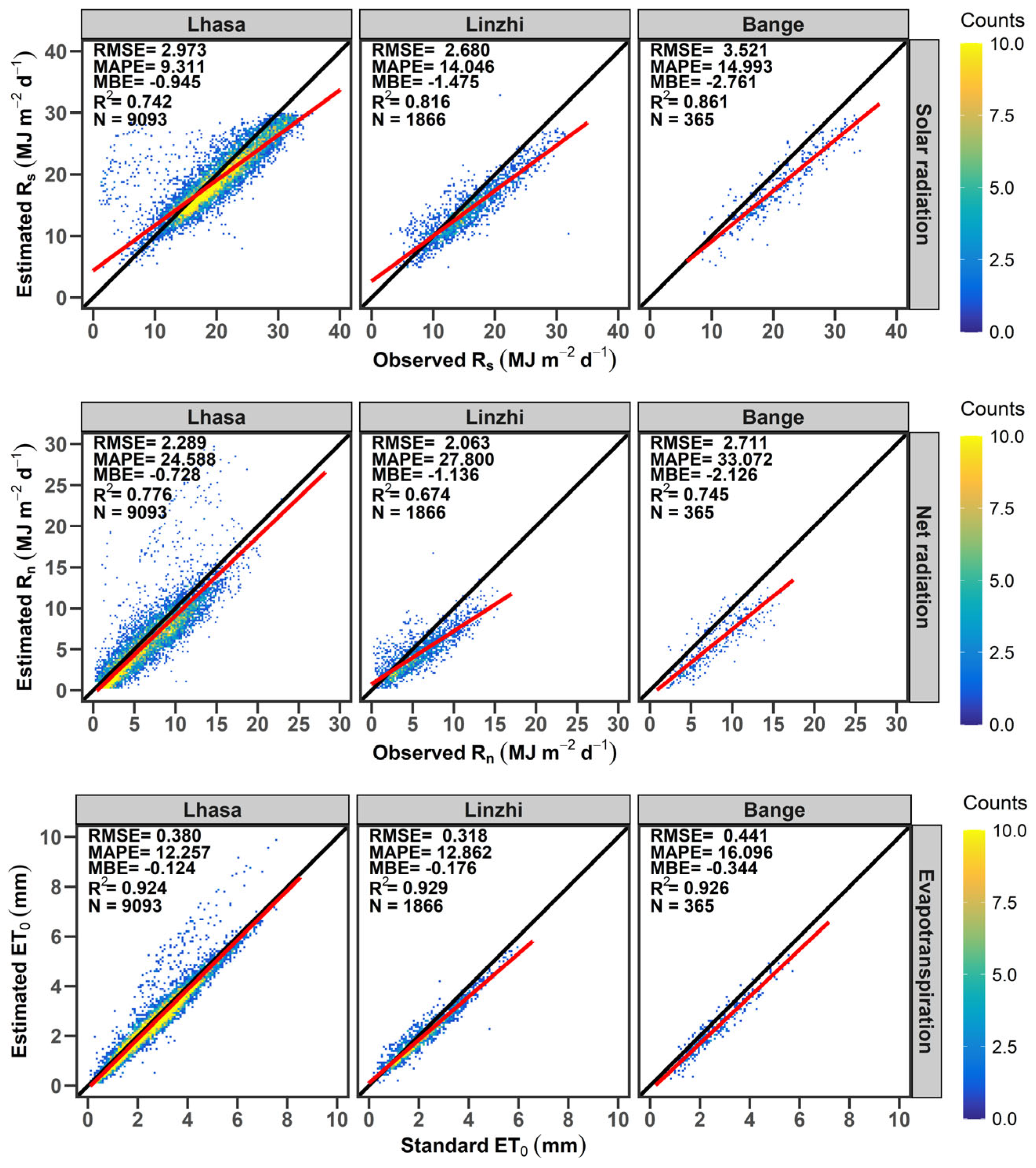
First, Rs was calculated using Fs. Then, the estimated Rs, along with all other measured data, including the measured Rnl, was used to drive the FAO56-PM. It is evident that the recommended Fs performed well in estimating Rs at all three stations, with R2 values of 0.742, 0.816, and 0.860 for Lhasa, Linzhi, and Bange, respectively (Figure 2). The negative values of MBE at all stations indicated that the recommended Fs, with its default coefficients, underestimated Rs over the TP. These errors in estimated Rs led to errors in estimated Rn, with negative MBE values of −0.728, −1.136, and −2.126 at Lhasa, Linzhi, and Bange, respectively (Figure 2). The errors in estimated Rn were further transmitted to errors in estimated ET0, with negative MBE values of −0.124, −0.176, and −0.344 at Lhasa, Linzhi, and Bange, respectively (Figure 2). Overall, the recommended Fs with its default coefficients underestimated Rs at all stations, resulting in underestimated Rn and ET0 accordingly.

3.1.2. Errors in Estimated ET0 Resulting from Recommended Fnl

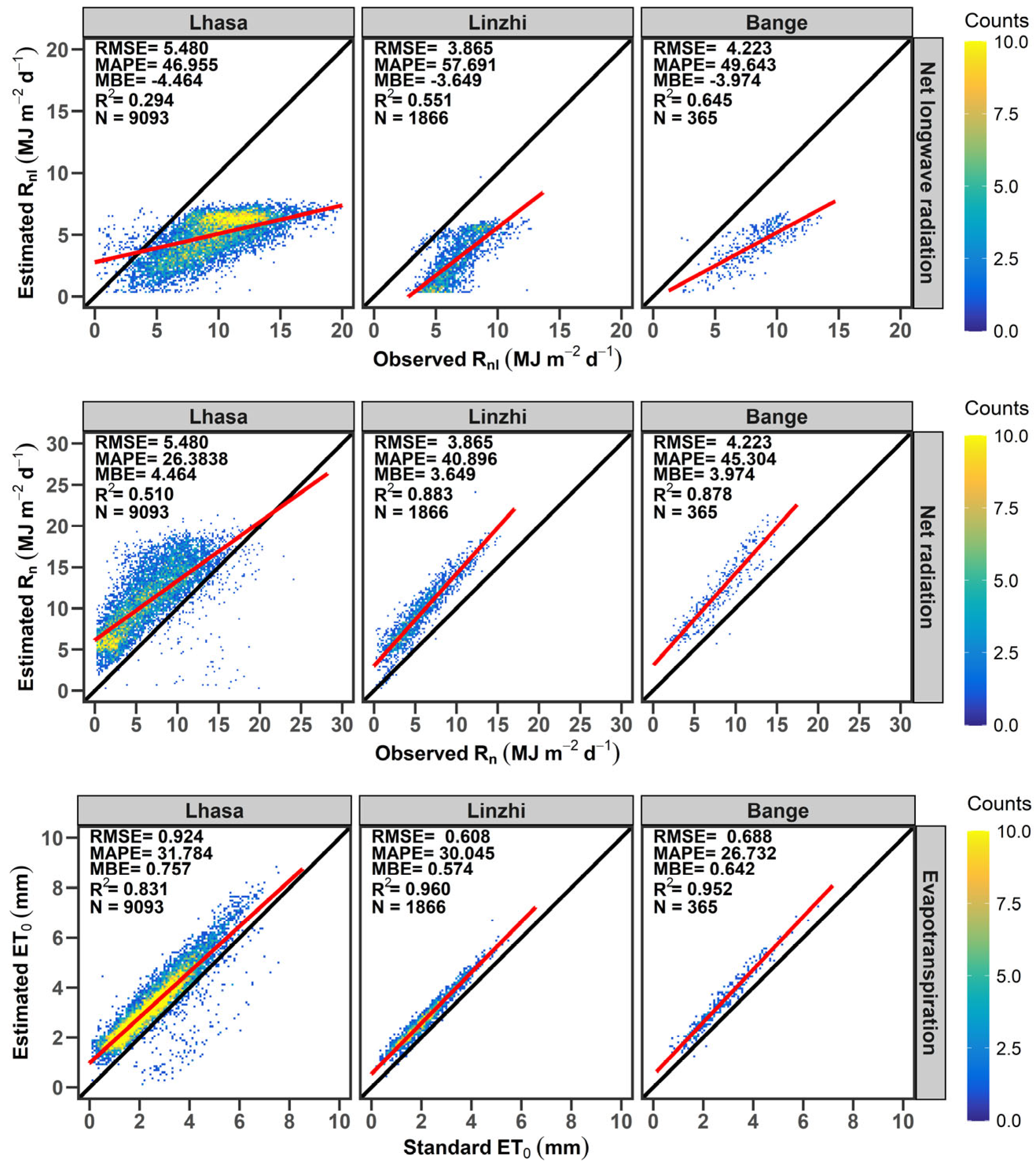
First, Rnl was estimated using Fnl with its default coefficients. Then, the estimated Rnl, along with all other measured data, including the measured Rs, was used to drive the FAO56-PM model. The recommended formula for Rnl performed poorly, with R2 values of 0.294, 0.551, and 0.654 for Lhasa, Linzhi, and Bange, respectively (Figure 3). Fnl significantly underestimated Rnl at all stations, with MBE values of −4.464, −3.649, and −3.974 for Lhasa, Linzhi, and Bange, respectively. As Rn was calculated as the difference between (1 − α)Rs and Rnl, i.e., (0.77RsRnl), and Rs was the measured data, the underestimated Rnl led to an overestimated Rn, which in turn resulted in an overestimated ET0 (Figure 3).

3.1.3. Errors in Estimated ET0 Resulting from Both Recommended Fs and Fnl

First, Rs and Rnl were calculated using Fs and Fnl, respectively. Then, these estimated values, along with other measured variables, were used to drive the FAO56-PM. This approach is essentially the AllenO method, which is the original FAO56-PM with its recommended formulas and default coefficients for estimating Rs and Rnl.
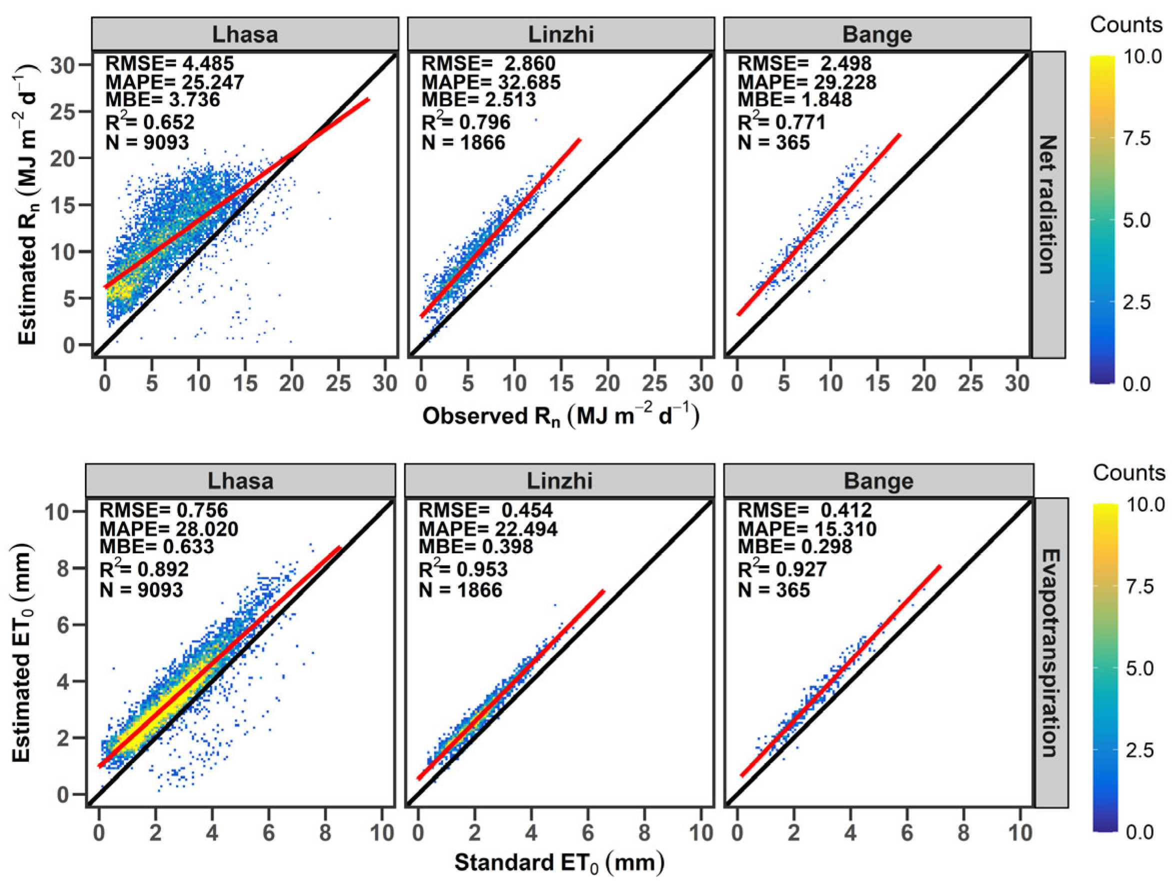
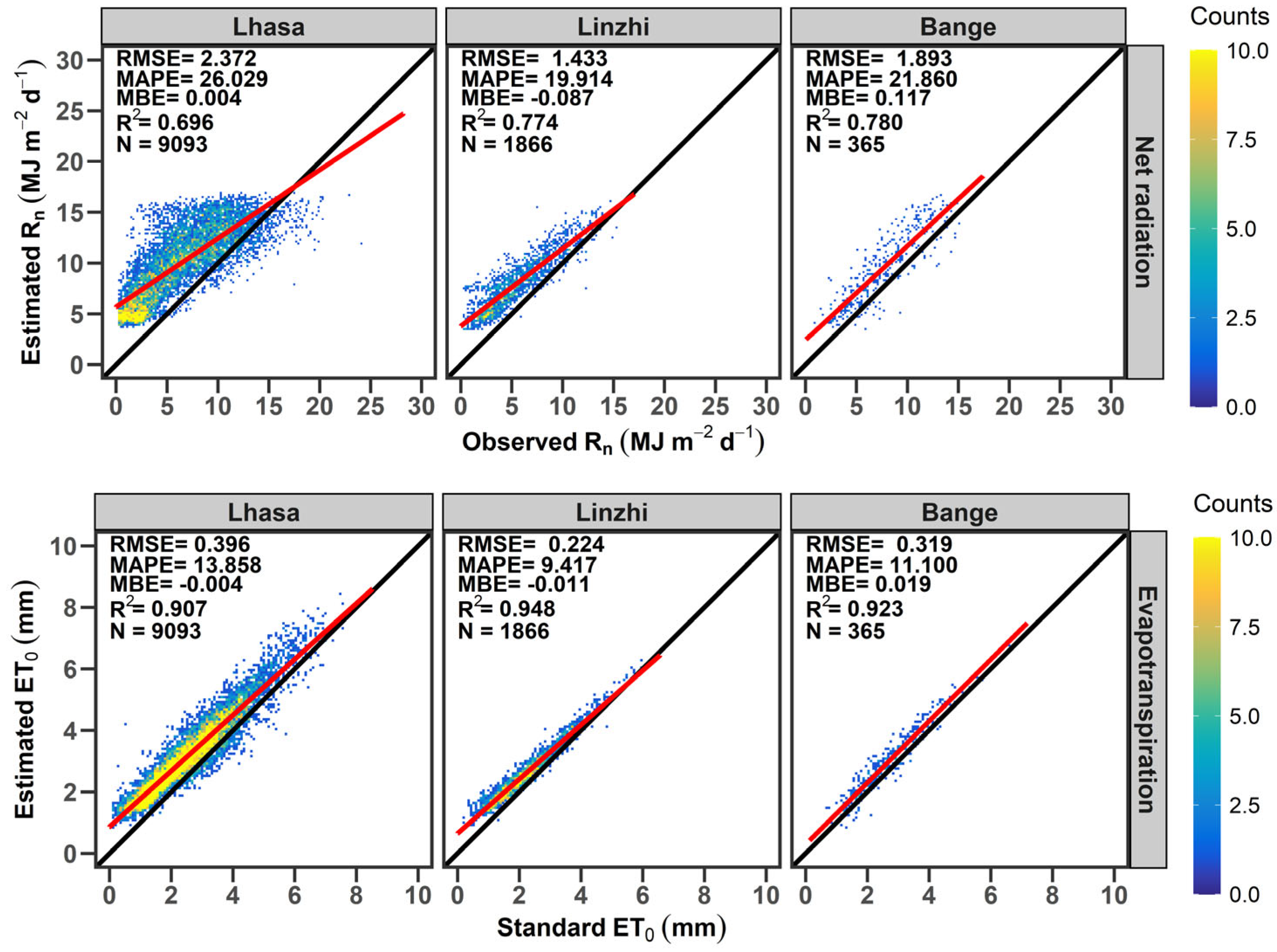
The errors in Rn (Figure 4) were due to both the estimated Rs (Figure 2) and the estimated Rnl (Figure 3). Rs was underestimated by Fs (Figure 2), while Rnl was even more significantly underestimated by Fnl (Figure 3). The larger negative MBE for Rnl was partly offset by the smaller negative MBE for Rs, resulting in a smaller MBE for Rn (Figure 4). Overall, Fnl caused a greater underestimation of Rnl compared to the underestimation of Rs by Fs. When both Rs and Rnl were estimated, the errors were offset partially, rather than accumulating, thus reducing the errors in Rn and increasing the accuracy in ET0.

3.2. Calibration of FAO56-PM

The original FAO56-PM, AllenO method, produced errors in the estimated ET0 due to its recommended Fs and Fnl with the default coefficients (Figure 4). Therefore, calibrating Fs and Fnl in AllenO became crucial for enhancing the performance of FAO56-PM.

3.2.1. Mere Calibration of the Recommended Fs

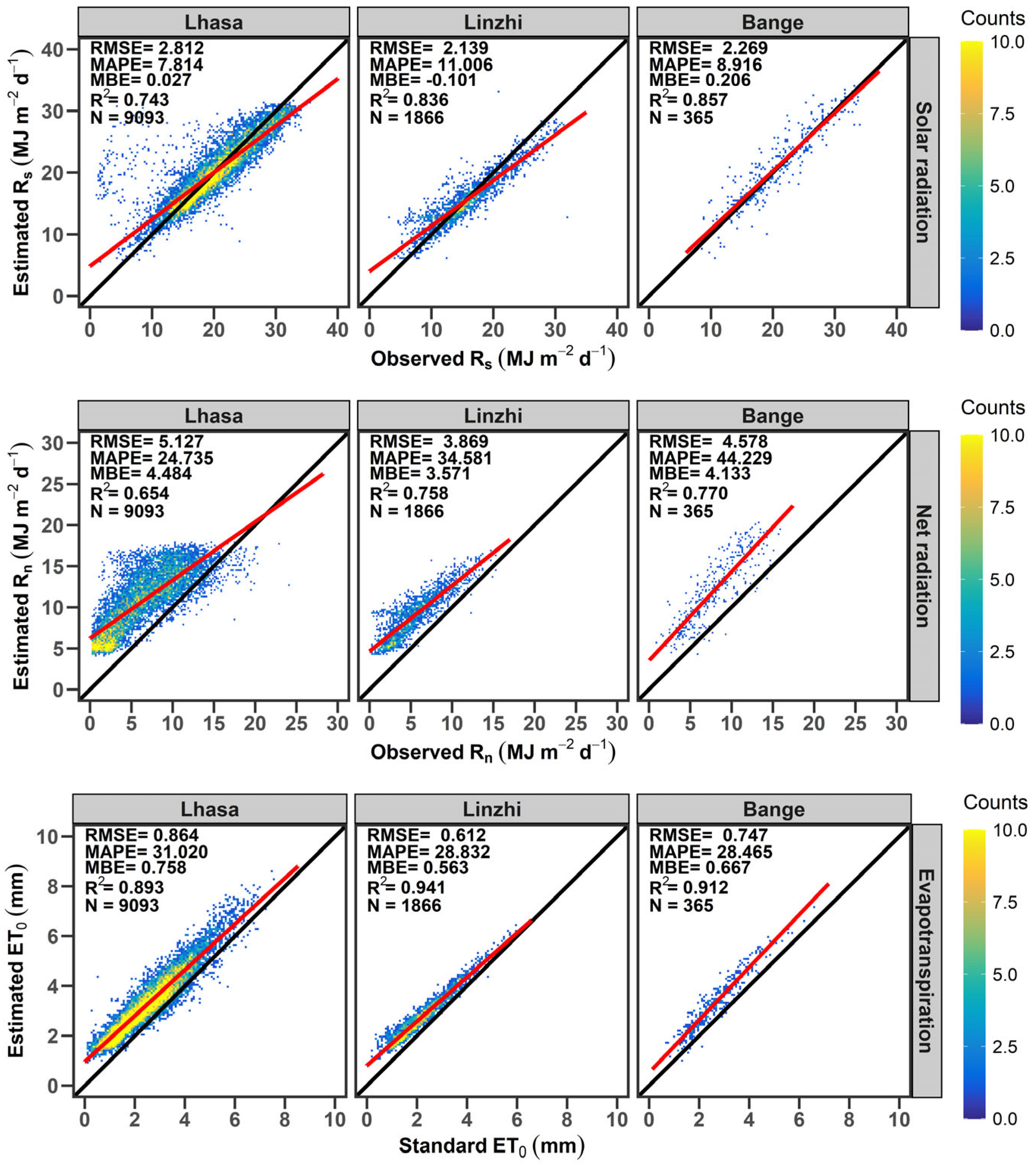
Calibration of only Fs was referred to as AllenS, which involved determining the coefficients a and b for Fs, as shown in Table 2. Compared to the original Fs (Figure 2), the calibrated Fs provided better estimates of Rs, evidenced by higher R2 values (Figure 5). Additionally, the calibrated Fs showed no significant discrepancies between measured and estimated Rs, with acceptable MBE values of 0.027, −0.101 and 0.206 for Lhasa, Linzhi and Bange, respectively (Figure 5). However, the original Fnl’s tendency to underestimate Rnl could not be compensated by the accurate estimation of Rs, resulting in a larger absolute MBE in Rn compared to AllenO (Figure 5 vs. Figure 4). In summary, while AllenS improved the accuracy of Rs estimation, it diminished the error offset between Fs and Fnl, thereby increasing errors in estimating Rn and ET0. Consequently, despite the effort put into the calibration process, AllenS performed worse than AllenO.

3.2.2. Mere Calibration of the Recommended Fnl

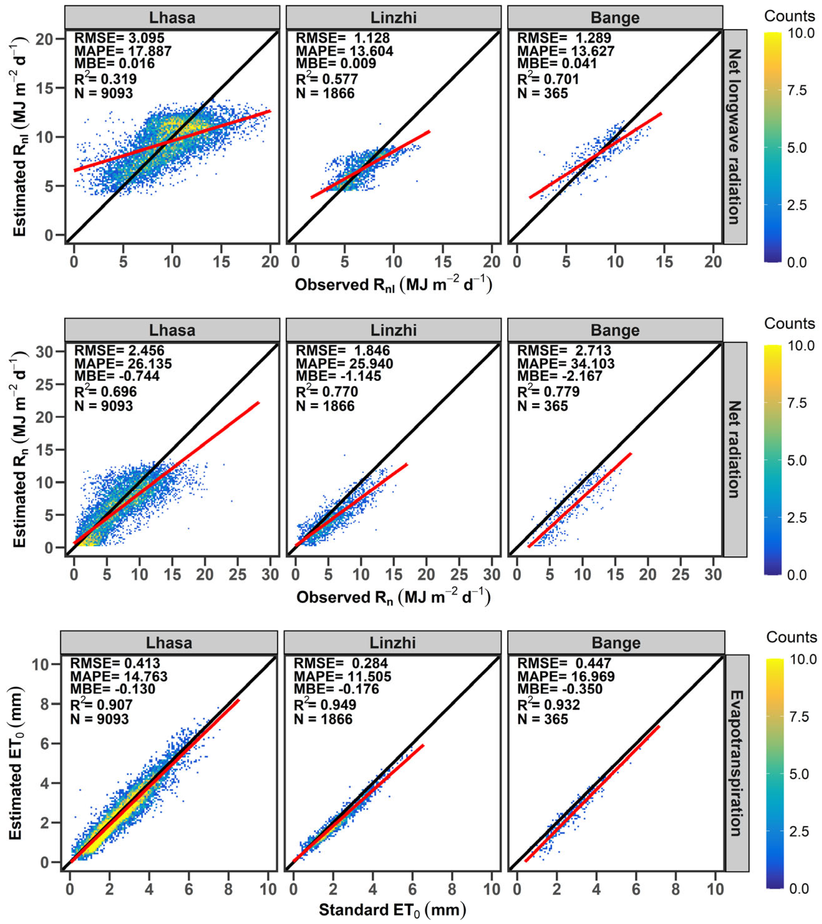
Calibration of only Fnl was referred to as AllenL. Table 2 shows the calibrated coefficients of c, d, e, and f for Fnl under AllenL. The calibrated Fnl outperformed the original Fnl, as demonstrated in Figure 2 and Figure 6, with higher R2 values of 0.319, 0.577, and 0.701, respectively. Compared to the original Fnl, the calibrated version significantly reduced systematic error in the estimated Rnl, achieving lower absolute MBE values of 0.016, 0.009, and 0.041 for Lhasa, Linzhi and Bange, respectively. After calibration of Fnl, errors in Rn were primarily due to Fs. Error analysis above indicated that the original Fnl was the main source of errors in Rn estimation, whereas Fs contributed comparatively minor errors (Figure 2 and Figure 3). Consequently, AllenL performed significantly better than AllenO. For AllenL, the system errors in Rn were notably small, with MBE values of −0.744, −1.145, and −2.167 for Lhasa, Linzhi and Bange, respectively. This enhanced accuracy in estimating Rn also improved the estimation of ET0 at all stations (Figure 6).

3.2.3. Comprehensive Calibration of Both Fs and Fnl

Only calibration of Fs or Fnl led to high accuracy in estimation of Rs or Rnl, respectively (Figure 5 and Figure 6). Thus, the comprehensive calibration of both Fs and Fnl, referred to as AllenC, resulted in small systemic errors in both the estimated Rs and the estimated Rnl (Figure 5 and Figure 6), leading to high accuracy in estimating Rn (Figure 7). Compared to AllenS and AllenL, AllenC produced smaller absolute MBE values for Rn at all stations (Figure 7). This high accuracy in Rn estimation also led to precise ET0 estimations, with MBE values of −0.004 at Lhasa, −0.011 at Linzhi, and 0.019 at Bange, respectively (Figure 7). In summary, AllenC significantly improved the accuracy of Rn and ET0 estimations compared to AllenO, AllenS, and AllenL methods.

3.3. General Method Developed for Regional Application of FAO56-PM over the TP

AllenC performed well in estimating Rn and ET0, but the calibrated coefficients for Fs and Fnl were site-specific, necessitating local calibration using measurements of both Rs and Rnl. In contrast, the coefficients of Fs and Fnl can be easily obtained by the general method of AllenR.
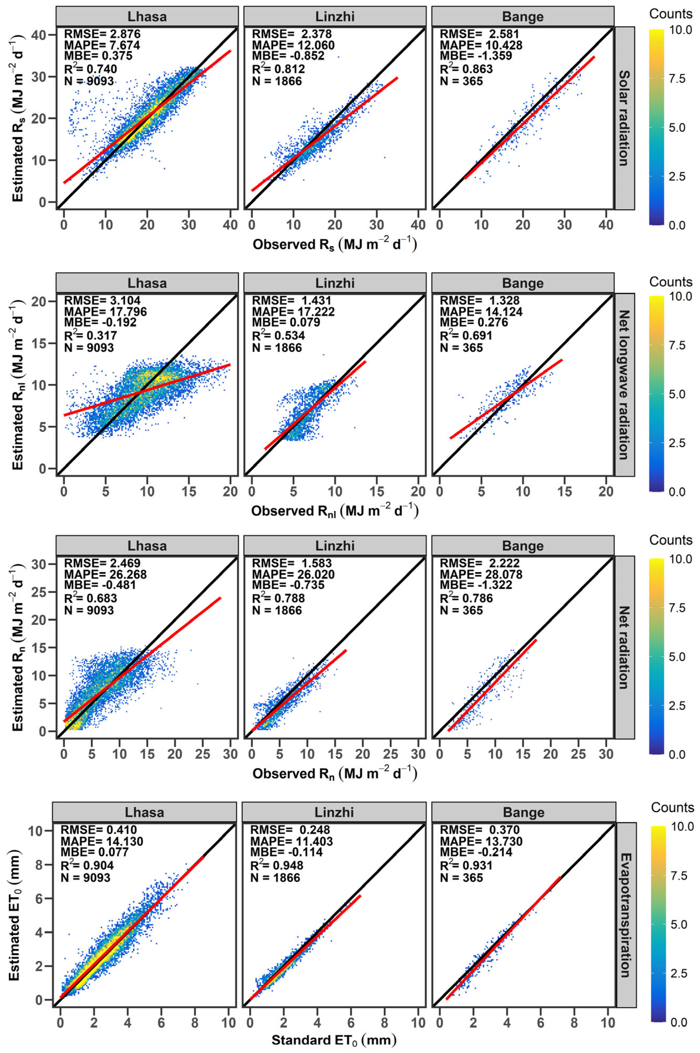
The coefficients for Fs and Fnl were calculated under the AllenR method, as shown in Table 2, and used to estimate Rs and Rnl (Figure 8). Compared to the errors in estimated Rs and Rnl using the original Fs and Fnl (Figure 2 and Figure 3), the errors using AllenR’s coefficients decreased significantly (Figure 8), indicating that AllenR outperformed the original FAO56-PM (AllenO) for estimating Rs and Rnl. This high accuracy in estimating Rs and Rnl contributed to the high accuracy in estimating Rn, which in turn led to accurate ET0 estimates (Figure 8). Naturally, the estimated Rs by AllenR was slightly less accurate than that by AllenS with local calibration, and the estimated Rnl by AllenR was also slightly less accurate than that by AllenL with local calibration (Figure 8 vs Figure 5 and Figure 6), which resulted in slightly larger errors in Rn and ET0 compared to the AllenC method. However, AllenR is still considered the most suitable method for regional ET0 estimation over the TP due to its higher accuracy than AllenO and broader applicability compared to AllenC.

3.4. Spatial Distribution of ET0 over the TP

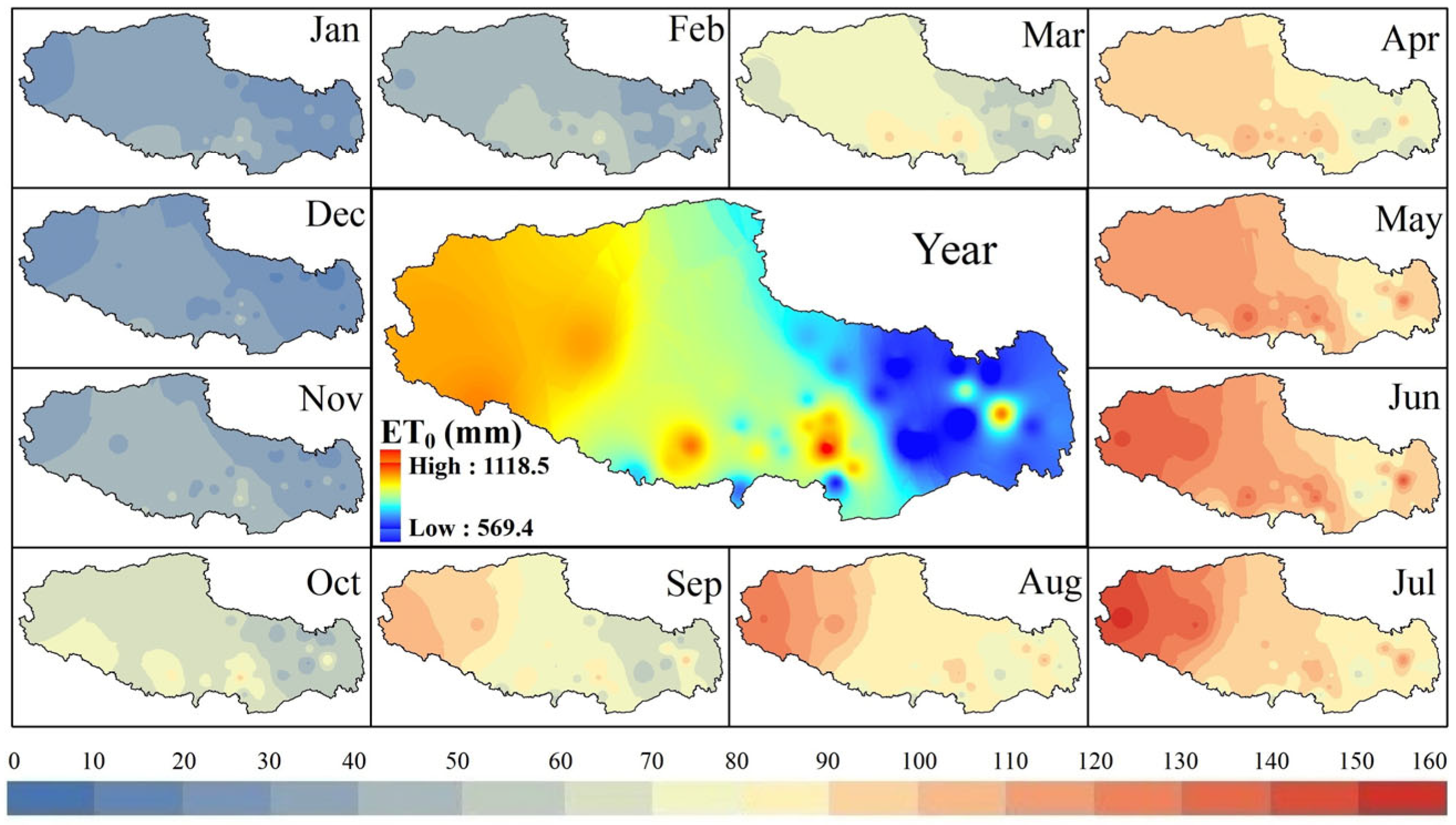
Meteorological data from 40 weather stations across the TP were used to estimate the regional ET0 using the AllenR method. From 1991 to 2020, the average annual ET0 ranged from 569 to 1118 mm, increasing from east to west, with some high values centered in Basu, Gongga, and Lazi (Figure 9). Within a year, the high monthly values predominantly occurred from April to September (Figure 9), coinciding with the growth period of highland barley in most areas of the TP.
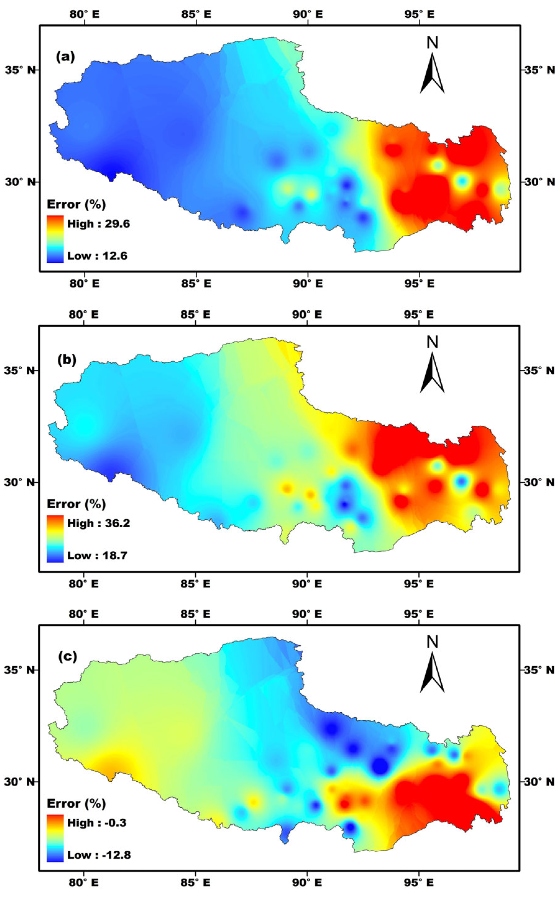
The estimated ET0 using AllenR was set as the base value (Vb), while estimates from other calibration methods were set as the compared values (Vc). The relative error in ET0 due to other methods was calculated as (Vc Vb)/Vb × 100%. According to AllenO’s calculations, ET0 was significantly overestimated, with the relative error decreasing from east to west, ranging from 12.6% to 29.6% (Figure 10a). The current popular method, AllenS, only calibration of Fs, produced a similar distribution pattern for the relative error, but the error increased, ranging from 18.8% to 36.2% (Figure 10b). Conversely, calibrating Fnl alone led to an underestimation of ET0, with the relative error ranging from −12.7% to −0.3%. The most significant underestimation occurred in southeastern Tibet, decreasing from southeast to northwest (Figure 10c).

3.5. Trend Analysis of ET0 over the TP

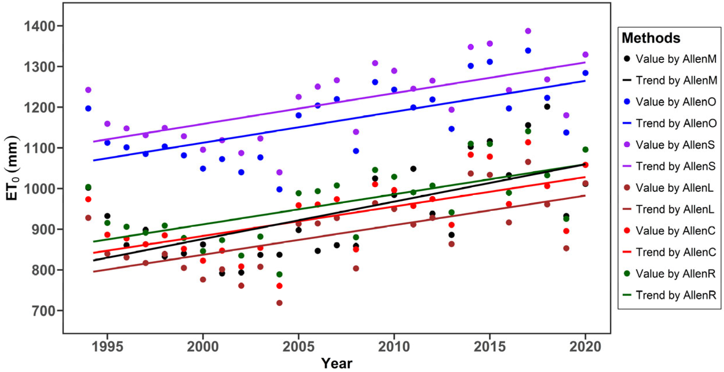
Trend analyses of ET0 at Lhasa from 1994 to 2020 were conducted using various calibration methods (Figure 11). When both Fs and Fnl were locally calibrated, AllenC outperformed all other methods. Calibrating only Fnl, the AllenL method performed worse than AllenC but significantly better than AllenO. The widely used AllenS method, which calibrates only Fs, performed even worse than AllenO. In contrast, AllenR performed slightly worse than AllenC but better than all other methods (Figure 11). Interestingly, the trends (slopes of regression lines) showed minimal differences among the calibration methods, with values of 9.1 mm/year for AllenM, 7.6 mm/year for AllenO, 7.5 mm/year for AllenS, 7.2 mm/year for AllenL, 7.2 mm/year for AllenC, and 7.3 mm/year for AllenR, respectively (Figure 11). Overall, different calibration methods led to significant variations in estimated ET0 but had only a minor impact on trend values.
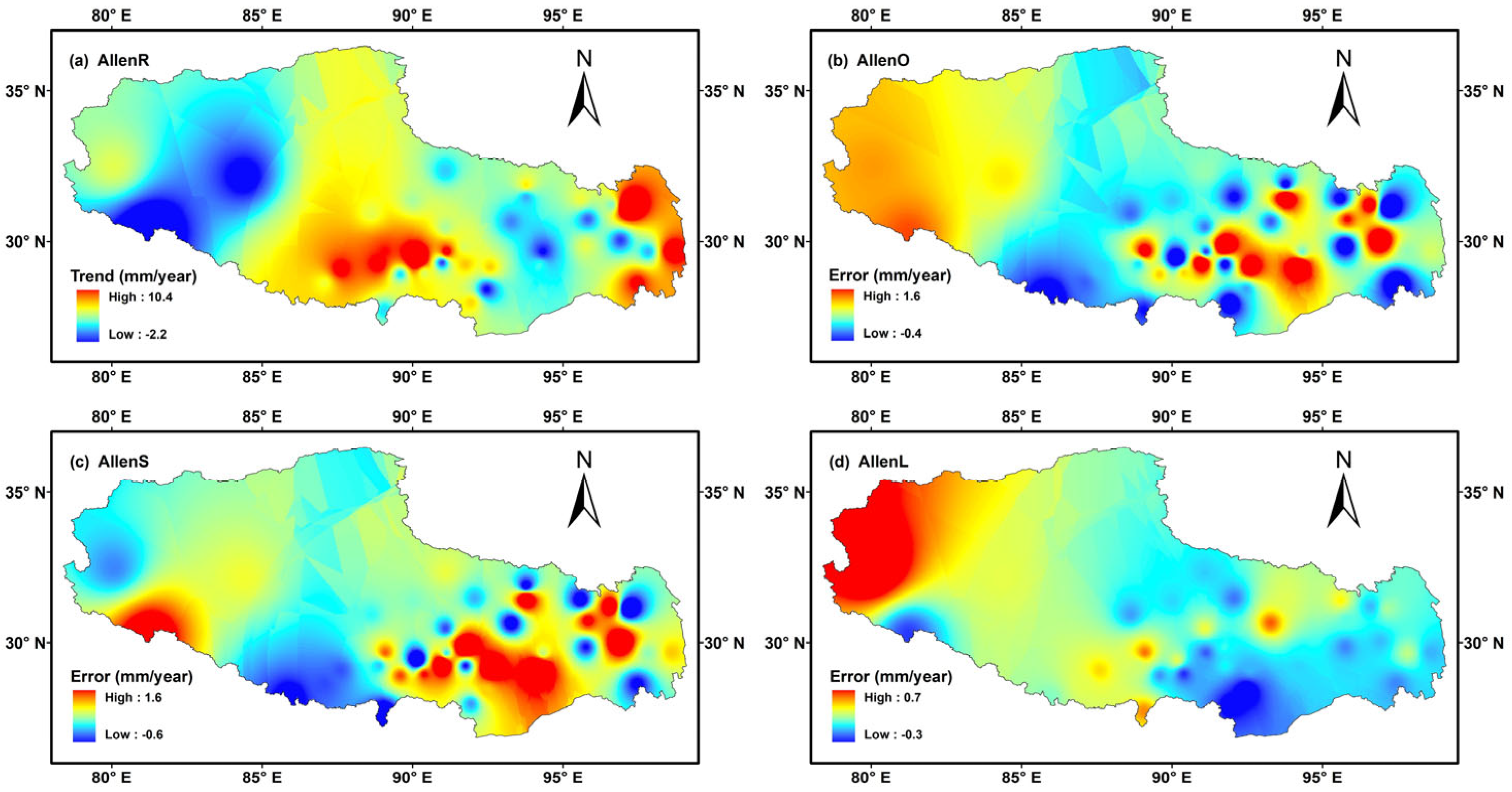
The spatial distribution of trends in ET0 from 1991 to 2000 was analyzed using the AllenR method. In the eastern and central parts of the TP, ET0 increased rapidly compared to other areas. Conversely, ET0 decreased in the western part of the TP over the past three decades (Figure 12a). Overall, ET0 showed increasing trends with an average value of 2.8 mm/year, ranging from −2.2 to 10.4 mm/year across the TP.
The AllenO method resulted in overestimated trends in ET0 in most regions of the TP (Figure 12b). The absolute error, calculated as (Vc Vb), averaged 0.51 mm/year, with values ranging from −0.4 to 1.6 mm/year (Figure 12b). AllenS produced a similar distribution of absolute error, ranging from −0.6 to 1.6 mm/year, with the largest errors occurring in the southeastern TP (Figure 12c). Conversely, AllenL led to a distinctly different distribution pattern of absolute error (Figure 12d). Trends in ET0 were underestimated in eastern TP but overestimated in western TP, with values ranging from −0.3 to 0.7 mm/year and an average of 0.1 mm/year across the TP.

4. Discussion

Various calibration methods led to discrepancies in the estimation of ET0. The widely used AllenS method, which involves only calibration of Fs, actually increased, rather than decreased, errors in the estimated ET0 over Tibet. These findings and their implications are discussed below.

4.1. High Rs and Rnl over the TP

The TP is known as the Third Pole of the world because of its high elevation [53,54,55]. The energy balance over the TP is notably distinct from that of the surrounding regions [56,57,58].
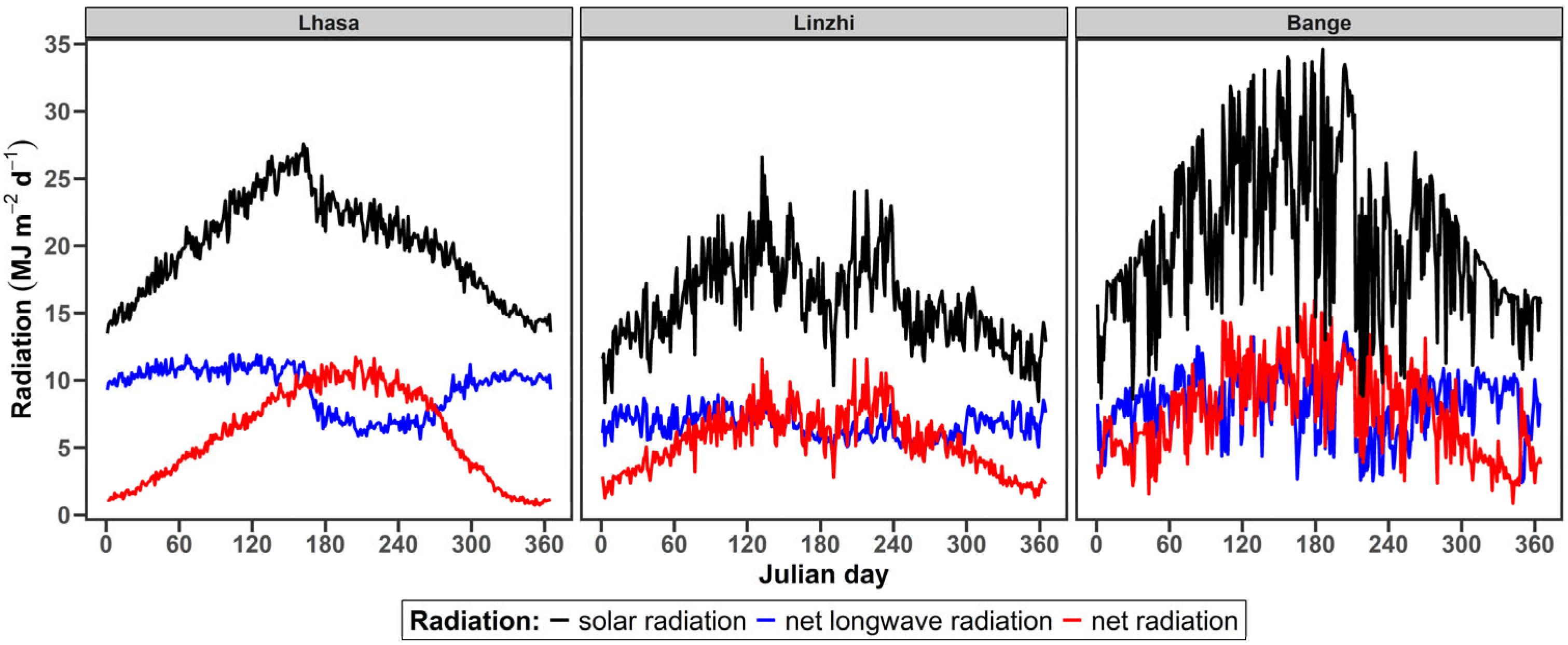
Radiation over the TP is significantly higher than that in surrounding regions [59,60,61], due to its high elevation and clear skies. The average daily radiation showed notably high values at Lhasa, Linzhi, and Bange (Figure 13), with mean values of 19.96 MJ m−2 d−1, 15.59 MJ m−2 d−1 and 20.61 MJ m−2 d−1, respectively. These radiation values are much higher than those measured at other stations with similar latitudes [62,63,64,65,66].
Rnl represents the difference between outgoing longwave radiation and incoming longwave radiation. Outgoing longwave radiation over the TP is slightly lower than that in surrounding areas due to the region’s lower temperature caused by high elevation [67]. In contrast, incoming longwave radiation is significantly lower due to clear sky conditions and low humidity in this highland area [68]. Consequently, Rnl over the TP is much higher than that in surrounding regions [69], which was also manifested in our study (Figure 13). The average Rnl values were 9.41, 6.62, and 8.17 MJ m−2 d−1 at Lhasa, Linzhi, and Bange, respectively (Figure 13), which are much higher than those in plains at similar latitudes [48,70,71]. Therefore, Rnl plays a crucial role in Rn over the TP [69], indicating that calibrating Fnl is essential for accurately estimating Rn and ET0 in this highland region.

4.2. Offsetting Effects Between Errors in Estimated Rs and Rnl

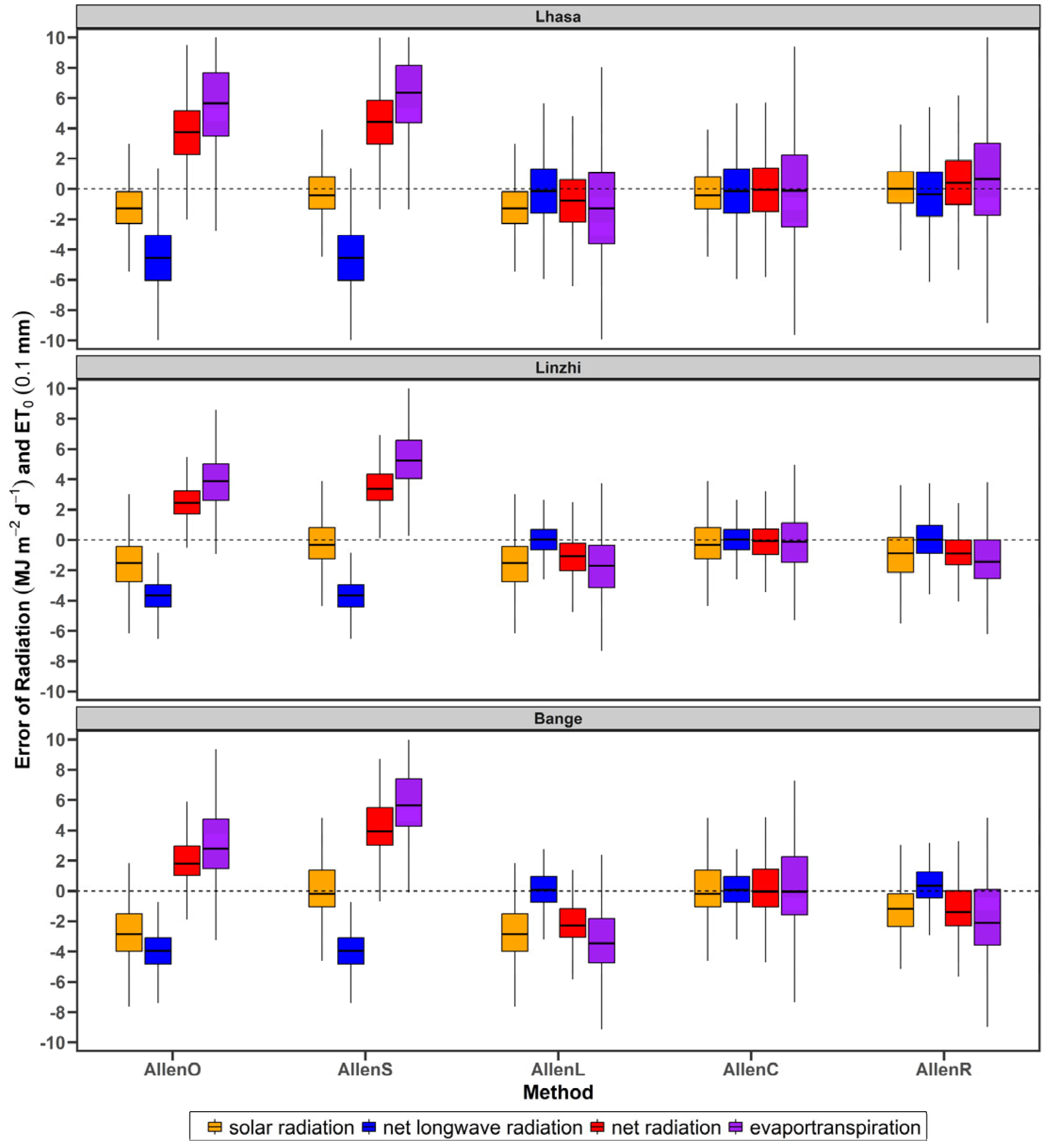
The original Fs and Fnl models were developed using data primarily collected from flat regions [17]. In contrast to the flat regions, the transmissions of solar radiation are approximately 10–15% greater over the plateau than those at sea-level stations because of its high altitude, thin air and good air transparency [72]. Therefore, the coefficients of b over the TP are usually greater than those in the other regions [41,73,74]. Thus, using Fs without calibration results in an underestimation of Rs over the TP [60], a finding corroborated in this study (Figure 2). Similarly, applying Fnl directly leads to an even greater underestimation of Rnl (Figure 3). In the FAO56-PM model, Rn is calculated as 0.77Rs minus Rnl. Consequently, the larger underestimation of Rnl partially offsets the smaller underestimation of Rs, leading to an overestimation of Rn at each station (Figure 4). The widely used AllenS method, which involves mere calibration of Fs, reduces this offsetting effect and further increases the overestimation of Rn (Figure 5). In contrast, mere calibration of Fnl (AllenL method) means that the primary errors in Rn estimation will mainly stem from Fs. Compared to Fnl, Fs contributes relatively smaller errors to Rn (Figure 2 and Figure 3), resulting in higher accuracy in estimating Rn and ET0 (Figure 6). Comprehensive calibration of both Fs and Fnl (AllenC method) yields very small errors in estimating both Rs and Rnl, leading to the best model performance in estimating Rn and ET0 (Figure 7). This offsetting effect can be intuitively observed in the errors of estimated Rs, Rnl, Rn and ET0 under different calculation methods (Figure 14).

4.3. Spatial Distribution and Temporal Trend of ET0 over the TP

According to AllenR, the spatial distribution of ET0 across TP increases from east to west, with notable high centers at Basu, Gongge, and Lazi (Figure 9). Previous studies using the original FAO56-PM (AllenO method) reported a very similar pattern [13]. Additionally, calibrating only Fs (AllenS) also produced a distribution pattern comparable to those of AllenR and AllenO [75]. However, compared to AllenR, AllenO resulted in a relative error range of 12.6% to 29.6%, while AllenS had an even higher error range of 18.8% to 36.2% over the TP (Figure 10a,b). These large estimation errors in ET0 could lead to impractical water management policies implemented by local governments [39].
Trend analysis by AllenR shows that ET0 has increased rapidly in the eastern part and decreased significantly in the western part of the TP (Figure 10a). This distribution pattern is similar to findings by AllenO [13] and AllenS [38,75,76], suggesting that different calibration methods of FAO56-PM may significantly affect the estimated ET0 values but have little impact on the trends in recent decades (see Figure 11). Therefore, we cautiously envisage that calibration methods have minimal influence on the results of ET0 trend analysis. Consequently, previous trend analyses by AllenO or AllenS may still be reliable [38,75,76], despite large errors in the estimated ET0 values [13].

4.4. Uncertainties and Future Studies

ET0 estimated by FAO56-PM is typically considered as the standard value for evaluating the performance of other empirical models in comparative studies (e.g., [21,33,34]). However, this study reveals that ET0 calculated using FAO56-PM is not a fixed value but varies depending on different calculation methods. Consequently, the standard ET0 used in previous studies may lead to confusion when assessing model performance. For instance, if the ET0 values are 1.0 mm/day, 2.0 mm/day, and 3.0 mm/day for AllenO, AllenS, and AllenM, respectively, and empirical models A, B, and C produce ET0 values of 1.0 mm/day, 2.0 mm/day, and 3.0 mm/day, respectively, model C would actually perform the best among the three models. However, if ET0 from AllenO or AllenS is used as the standard value (e.g., [33,34]), the evaluation results could differ significantly. Therefore, the standard ET0 used in past studies might lead to unreliable conclusions about model performance. Future research should reevaluate these findings.
In recent years, uncertainty analysis of ET0 under climate change scenarios has become a significant research focus [77,78,79]. Typically, ET0 calculated using the FAO56-PM method serves as a benchmark for assessing uncertainties from Global Climate Models (GCMs) and climate change scenarios [80,81,82]. However, as discussed above, ET0 derived from FAO56-PM can vary depending on the calculation method used. When calculated using the original FAO56-PM (AllenO), the maximum relative error in ET0 estimation can reach up to 29.6% (Figure 10a). Consequently, the benchmark itself is uncertain, and this uncertainty has not been accounted for in current analyses [80,81,82]. To mitigate this issue, the benchmark for ET0 should be determined using FAO56-PM with comprehensive calibration of both Fs and Fnl. Additionally, ET0 plays a crucial role in various drought indices [83,84,85], hydrological models [86,87,88], and crop growth models [7,8,9]. The outcomes of these indices or models may be affected by different calculation methods for FAO56-PM, a factor that should be addressed in future research. Furthermore, we observed that FAO56-PM is often briefly mentioned in related literature without details on the description of the data for Rs and Rnl (e.g., [80,82]). Given that the estimated ET0 is significantly influenced by the calculation methods for Rs and Rnl, we strongly recommend that all authors clearly specify the methods used for calculating Rs and Rnl in future studies involving FAO56-PM.
As revealed in this study, Rnl plays a very important role in estimating Rn, a finding also identified in other studies [45,46,89]. However, compared to the accurate estimation of Rs by the calibrated Fs (Figure 3), Fnl performed worse in estimating Rnl over the TP in this study, even with calibrated coefficients (Figure 4). Our findings are consistent with previous reports [47,90], which indicated that Rnl was also underestimated in other locations. Therefore, simultaneous calibration of both Rs and Rnl based on local conditions is crucial for accurately estimating Rn and ET0 [89,91,92]. In addition, Kofronova et al. [90] used different empirical models to estimate Rnl, showing that empirical models for Fnl exhibited large RMSE values with calibrated coefficients, which agrees well with our findings. Therefore, new methods should be developed for accurate estimation of Rnl to improve the model performance of FAO56-PM in future studies, incorporating current popular approaches based on various machine learning models [41,93,94,95]. Additionally, though the FAO56-PM is considered the most reliable method for calculating ET0, direct validation of the FAO56-PM against observed measurements from lysimeters and similar instruments is also crucial. This should be an important scientific task for future work over the Tibetan Plateau.

5. Conclusions

Both Rs and Rnl values are significantly higher over the TP compared to surrounding regions. The formulas for Rs and Rnl recommended in the original FAO56-PM led to underestimations of both values, with Rnl being more significantly underestimated than Rs.
Comprehensive calibration of the formulas for both Rs and Rnl led to the best performance of the FAO56-PM. The general calibration model, using coefficients derived from readily available geographical and basic meteorological parameters, was slightly less effective than local calibration of the formulas for both Rs and Rnl, but obviously outperformed the original FAO56-PM, demonstrating significant regional applicability over the TP. Compared to the original FAO56-PM, mere calibration of the formula for Rnl notably improves accuracy in estimating ET0, whereas only calibration of the formula for Rs reduces, rather than improves, the accuracy due to the diminished offsetting effect between underestimated Rs and Rnl.
The general model calculated that ET0 increased from east to west, ranging from 569.4 mm/year to 1118.5 mm/year. Other calculation methods showed a similar spatial distribution pattern, with relative errors in ET0 ranging from 12.6% to 29.6% under the original FAO56-PM. Trend analysis revealed that ET0 increased rapidly in the eastern region while decreasing significantly in the western region of the TP over recent decades. Interestingly, although different calculation methods affect the estimated values of ET0, they have minimal impact on the trend analysis results.

Author Contributions

Conceptualization, J.L., G.Z., J.D., M.L., Y.S., S.C. and Y.J.; methodology, J.L., G.Z., J.D., M.L., Y.S., S.C. and Y.J.; software, J.L.; validation, G.Z. and J.D.; formal analysis, Y.S.; writing—original draft preparation, J.L.; writing—review and editing, G.Z. All authors have read and agreed to the published version of the manuscript.

Funding

This research was supported by the Tibet Science and Technology Plan Major Special Project (No. XZ202402ZD0006-02) and the Natural Science Foundation of China (No. 42330602).

Institutional Review Board Statement

Not applicable.

Informed Consent Statement

Not applicable.

Data Availability Statement

There are no relevant statements for this research.

Acknowledgments

The authors would like to thank the observers over the Tibetan Plateau for their experiments conducted under extremely harsh environments.

Conflicts of Interest

The authors declare no conflicts of interest.

References

  1. Mondal, S.; Mishra, A. Quantifying the precipitation, evapotranspiration, and soil moisture network’s interaction over global land surface hydrological cycle. Water Resour. Res. 2024, 60, e2023WR034861. [Google Scholar] [CrossRef]
  2. Hu, S.; Gao, R.; Zhang, T.; Bai, P.; Zhang, R. Spatio-temporal variation of reference evapotranspiration and its climatic drivers over the Tibetan Plateau during 1970–2018. Appl. Sci. 2021, 11, 8013. [Google Scholar] [CrossRef]
  3. Zhao, F.; Ma, S.; Wu, Y.; Qiu, L.; Wang, W.; Lian, Y.; Chen, J.; Sivakumar, B. The role of climate change and vegetation greening on evapotranspiration variation in the Yellow River Basen, China. Agric. For. Meteorol. 2022, 316, 108842. [Google Scholar] [CrossRef]
  4. Koutsoyiannis, D. Revisiting the global hydrological cycle: Is it intensifying? Hydrol. Earth Syst. Sci. 2020, 24, 3899–3932. [Google Scholar] [CrossRef]
  5. Labat, D. Oscillations in land surface hydrological cycle. Earth Planet. Sci. Lett. 2006, 242, 143–154. [Google Scholar] [CrossRef]
  6. Rast, M.; Johannessen, J.; Mauser, W. Review of understanding of Earth’s hydrological cycle: Observations, theory and modelling. Surv. Geophys. 2014, 35, 491–513. [Google Scholar] [CrossRef]
  7. Bouman, B.A.M.; Van Keulen, H.; Van Laar, H.H.; Rabbinge, R. The ‘School of de Wit’crop growth simulation models: A pedigree and historical overview. Agric. Syst. 1996, 52, 171–198. [Google Scholar] [CrossRef]
  8. Jones, J.W.; Hoogenboom, G.; Porter, C.H.; Boote, K.J.; Batchelor, W.D.; Hunt, L.A.; Wilkens, P.W.; Singh, U.; Gijsman, A.J.; Ritchie, J.T. The DSSAT cropping system model. Eur. J. Agron. 2003, 18, 235–265. [Google Scholar] [CrossRef]
  9. Keating, B.A.; Carberry, P.S.; Hammer, G.L.; Probert, M.E.; Robertson, M.J.; Holzworth, D.; Huth, N.I.; Hargreaves, J.N.G.; Meinke, H.; Hochman, G. An overview of APSIM, a model designed for farming systems simulation. Eur. J. Agron. 2003, 18, 267–288. [Google Scholar] [CrossRef]
  10. Bogawski, P.; Bednorz, E. Comparison and validation of selected evapotranspiration models for conditions in Poland (Central Europe). Water Resour. Manag. 2014, 28, 5021–5038. [Google Scholar] [CrossRef]
  11. Chen, A.; Orlov-Levin, V.; Meron, M. Applying high-resolution visible-channel aerial imaging of crop canopy to precision irrigation management. Agric. Water Manag. 2019, 216, 196–205. [Google Scholar] [CrossRef]
  12. Gao, H.; Liu, J.; Wang, H.; Mei, C.; Wang, J. Estimation of irrigated crop artificial irrigation evapotranspiration in China. Sci. Rep. 2024, 14, 16142. [Google Scholar] [CrossRef]
  13. Tang, P.; Xu, B.; Tian, D.; Ren, J.; Li, Z. Temporal and spatial variations of meteorological elements and reference crop evapotranspiration in Alpine regions of Tibet, China. Environ. Sci. Pollut. Res. 2021, 28, 36076–36091. [Google Scholar] [CrossRef]
  14. Liu, X.; Xu, C.; Zhong, X.; Li, Y.; Yuan, X.; Cao, J. Comparison of 16 models for reference crop evapotranspiration against weighing lysimeter measurement. Agric. Water Manag. 2017, 184, 145–155. [Google Scholar] [CrossRef]
  15. Zhao, W.L.; Qiu, G.Y.; Xiong, Y.J.; Paw U, K.T.; Gentine, P.; Chen, B.Y. Uncertainties caused by resistances in evapotranspiration estimation using high-density eddy covariance measurements. J. Hydrometeorol. 2020, 21, 1349–1365. [Google Scholar] [CrossRef]
  16. Azhar, A.H.; Perera, B.J.C. Evaluation of reference evapotranspiration estimation methods under Southeast Australian conditions. J. Irrig. Drain. Eng. 2011, 137, 268–279. [Google Scholar] [CrossRef]
  17. Allen, R.G.; Pereira, L.S.; Raes, D.; Smith, M. Crop Evapotranspiration—Guidelines for Computing Crop Water Requirements–FAO Irrigation and Drainage Paper 56; Food and Agriculture Organization of the United Nations: Rome, Italy, 1998. [Google Scholar]
  18. Anda, A.; Soos, G.; da Silva, J.A.T.; Kozma-Bognar, V. Regional evapotranspiration from a wetland in Central Europe, in a 16-year period without human intervention. Agric. For. Meteorol. 2015, 205, 60–72. [Google Scholar] [CrossRef]
  19. Doorenbos, J.; Pruitt, W.O. Guidelines for Predicting Crop Water Requirements. FAO Irrigation and Drainage Paper 24; Food and Agriculture Organization of the United Nations: Rome, Italy, 1977. [Google Scholar]
  20. Xue, Y.; Zhang, Z.; Li, X.; Liang, H.; Yin, L. A review of evapotranspiration estimation models: Advances and future development. Water Resour. Manag. 2025, 39, 3641–3657. [Google Scholar] [CrossRef]
  21. Tabari, H.; Grismer, M.E.; Trajkovic, S. Comparative analysis of 31 reference evapotranspiration methods under humid conditions. Irrig. Sci. 2013, 31, 107–117. [Google Scholar] [CrossRef]
  22. Monteith, J.L. Evaporation and environment. In Symposia of the Society for Experimental Biology; Cambridge University Press (CUP): Cambridge, UK, 1965. [Google Scholar]
  23. Penman, H.L. Natural evaporation from open water, bare soil and grass. Proc. R. Soc. Lond. 1948, 193, 120–145. [Google Scholar]
  24. Jensen, M.E.; Haise, H.R. Estimating evapotranspiration from solar radiation. J. Irrig. Drain. Div. 1963, 89, 15–41. [Google Scholar] [CrossRef]
  25. Priestley, C.H.B.; Taylor, R.J. On the assessment of surface heat flux and evaporation using large-scale parameters. Mon. Weather Rev. 1972, 100, 81–92. [Google Scholar] [CrossRef]
  26. Turc, L. Evaluation des besoins en eau irrigation, l’evapotranspiration potentielle. Ann. Agron. 1961, 12, 13–49. [Google Scholar]
  27. Hargreaves, G.L.; Hargreaves, G.H.; Riley, J.P. Irrigation water requirements for Senegal River basin. J. Irrig. Drain. Eng. 1985, 111, 265–275. [Google Scholar] [CrossRef]
  28. Thornthwaite, C.W. An approach toward a rational classification of climate. Geogr. Rev. 1948, 38, 55–94. [Google Scholar] [CrossRef]
  29. Xu, C.Y.; Singh, V.P. Cross comparison of empirical equations for calculating potential evapotranspiration with data from Switzerland. Water Resour. Manag. 2002, 16, 197–219. [Google Scholar] [CrossRef]
  30. Dalton, J. Experimental essays on the constitution of mixed gases. Manch. Lit. Philos. Soc. Memo 1802, 5, 535–602. [Google Scholar]
  31. Mahringer, W. Verdunstungsstudien am neusiedler See. Arch. Für Meteorol. Geophys. Und Bioklimatol. Ser. B 1970, 18, 1–20. [Google Scholar] [CrossRef]
  32. Singh, V.P.; Xu, C.Y. Evaluation and generalization of 13 masstransfer equations for determining free water evaporation. Hydrol. Process. 1997, 11, 311–323. [Google Scholar] [CrossRef]
  33. Chen, D.; Gao, G.; Xu, C.; Guo, J.; Ren, G. Comparison of the Thornthwaite method and pan data with the standard Penman–Monteith estimates of reference evapotranspiration in China. Clim. Res. 2005, 28, 123–132. [Google Scholar] [CrossRef]
  34. Liu, X.; Lin, E. Performance of the Priestley-Taylor equation in the semiarid climate of North China. Agric. Water Manag. 2005, 71, 1–17. [Google Scholar]
  35. Milly, P.C.D.; Dunne, K.A. Potential evapotranspiration and continental drying. Nat. Clim. Change 2016, 6, 946. [Google Scholar] [CrossRef]
  36. Sentelhas, P.C.; Gillespie, T.J.; Santos, E.A. Evaluation of FAO Penman–Monteith and alternative methods for estimating reference evapotranspiration with missing data in Southern Ontario, Canada. Agric. Water Manag. 2010, 97, 635–644. [Google Scholar] [CrossRef]
  37. Trajkovic, S.; Kolakovic, S. Evaluation of reference evapotranspiration equations under humid conditions. Water Resour. Manag. 2009, 23, 3057–3067. [Google Scholar] [CrossRef]
  38. Chen, S.; Liu, Y.; Thomas, A. Climatic change on the Tibetan Plateau: Potential evapotranspiration trends from 1961-2000. Clim. Change 2006, 76, 291–319. [Google Scholar]
  39. Liu, X.; Mei, X.; Li, Y.; Wang, Q.; Zhang, Y.; Porter, J.R. Variation in reference crop evapotranspiration caused by the Angstrom-Prescott coefficient: Locally calibrated versus the FAO recommended. Agric. Water Manag. 2009, 96, 1137–1145. [Google Scholar] [CrossRef]
  40. Yin, Y.; Wu, S.; Zheng, D.; Yang, Q. Radiation calibration of FAO56 Penman-Monteith model to estimate reference crop evapotranspiration in China. Agric. Water Manag. 2008, 95, 77–84. [Google Scholar] [CrossRef]
  41. Chen, S.; He, C.; Huang, Z.; Xu, X.; Jiang, T.; He, Z.; Liu, J.; Su, B.; Fenf, H.; Yu, Q.; et al. Using support vector machine to deal with the missing of solar radiation data in daily reference evapotranspiration estimation in China. Agric. For. Meteorol. 2022, 316, 108864. [Google Scholar] [CrossRef]
  42. Cunha, A.C.; Gabriel Filho, L.R.A.; Tanaka, A.A.; Goes, B.C.; Putti, F.F. Influence of the estimated global solar radiation on the reference evapotranspiration obtained through the penman-monteith fao 56 method. Agric. Water Manag. 2021, 243, 106491. [Google Scholar] [CrossRef]
  43. Paredes, P.; Pereira, L.S. Computing FAO56 reference grass evapotranspiration PM-ET0 from temperature with focus on solar radiation. Agric. Water Manag. 2019, 215, 86–102. [Google Scholar] [CrossRef]
  44. Sabziparvar, A.A.; Mousavi, R.; Marof, S.; Ebrahimipak, N.A.; Heidari, M. An improved estimation of the Angstrom-Prescott radiation coefficients for the FAO56 Penman-Monteith evapotranspiration method. Water Resour. Manag. 2013, 27, 2839–2854. [Google Scholar] [CrossRef]
  45. Duarte, H.F.; Dias, N.L.; Maggiotto, S.R. Assessing daytime downward longwave radiation estimates for clear and cloudy skies in Southern Brazil. Agric. For. Meteorol. 2006, 139, 171–181. [Google Scholar] [CrossRef]
  46. Kjaersgaard, J.H.; Plauborg, F.L.; Hansen, S. Comparison of models for calculating daytime long-wave irradiance using long term data set. Agric. For. Meteorol. 2007, 143, 49–63. [Google Scholar] [CrossRef]
  47. Matsui, H.; Osawa, K. Calibration effects of the net longwave radiation equation in Penman-type methods at Tateno, Japan. Hydrol. Res. Lett. 2015, 9, 113–117. [Google Scholar] [CrossRef]
  48. Zhu, X.; Qiu, X.; Zeng, Y.; Ren, W.; Tao, B.; Gao, J.; Liu, H.; Tan, Y. Effects of complex terrain on net surface longwave radiation in China. Theor. Appl. Climatol. 2018, 134, 251–264. [Google Scholar] [CrossRef]
  49. Liu, Z.F.; Yao, Z.J.; Yu, C.Q.; Zhong, Z.M. Assessing crop water demand and deficit for the growth of spring highland barley in Tibet, China. J. Integr. Agric. 2013, 12, 541–551. [Google Scholar] [CrossRef]
  50. Li, J.; Lu, C.; Chen, J.; Zhou, X.; Yang, K.; Li, J.; Wu, X.; Wu, S.; Hu, R.; Zhou, Z.; et al. The influence of complex terrain on cloud and precipitation on the foot and slope of the southeastern Tibetan Plateau. Clim. Dyn. 2024, 62, 3143–3163. [Google Scholar] [CrossRef]
  51. Liu, J.; Pan, T.; Chen, D.; Zhou, X.; Yu, Q.; Flerchinger, G.N.; Shen, Y. An improved Ångström-type model for estimating solar radiation over the Tibetan Plateau. Energies 2017, 10, 892. [Google Scholar] [CrossRef]
  52. Hans, V.S.; Francos, W.Z. Statistical Analysis in Climate Research; Cambridge University Press: Cambridge, UK, 1999. [Google Scholar]
  53. Pan, X.; Guo, X.; Li, X.; Niu, X.; Yang, X.; Feng, M.; Che, T.; Jin, R.; Ran, Y.; Guo, J.; et al. National Tibetan Plateau Data Center: Promoting earth system science on the third pole. Bull. Am. Meteorol. Soc. 2021, 102, E2062–E2078. [Google Scholar] [CrossRef]
  54. Qian, X.; Yao, Y.; Wang, H.; Zou, L.; Li, Y. Statistics and analysis of high-altitude wind above the western Tibetan Plateau. Mon. Not. R. Astron. Soc. 2020, 498, 5786–5797. [Google Scholar] [CrossRef]
  55. Yao, T.; Thompson, L.; Chen, D.; Piao, S. Reflections and future strategies for third pole environment. Nat. Rev. Earth Environ. 2022, 3, 608–610. [Google Scholar] [CrossRef]
  56. Deng, M.; Meng, X.; Sheng, D.; Niu, H.; Wu, P.; Li, Z.; Chen, H.; Shang, L.; Wang, S.; Lyu, S. Observed surface heat fluxes partitioning during the local growing season over the Tibetan Plateau. Agric. For. Meteorol. 2024, 356, 110186. [Google Scholar] [CrossRef]
  57. Duan, A.; Wang, M.; Lei, Y.; Cui, Y. Trends in summer rainfall over China associated with the Tibetan Plateau sensible heat source during 1980-2008. J. Clim. 2013, 26, 261–275. [Google Scholar] [CrossRef]
  58. Yao, J.; Gu, L.; Yang, C.; Chen, H.; Wang, J.; Ding, Y.; Li, R.; Zhao, L.; Xiao, Y.; Qiao, Y.; et al. Estimation of surface energy fluxes in the permafrost region of the Tibetan Plateau based on in situ measurements and the surface energy balance system model. Int. J. Climatol. 2020, 40, 5783–5800. [Google Scholar] [CrossRef]
  59. Li, H.; Ma, W.; Lian, Y.; Wang, X.; Zhao, L. Global solar radiation estimation with sunshine duration in Tibet, China. Renew. Energy 2011, 36, 3141–3145. [Google Scholar] [CrossRef]
  60. Liu, J.; Liu, J.; Linderholm, H.W.; Chen, D.; Yu, Q.; Wu, D.; Haginoya, S. Observation and calculation of the solar radiation on the Tibetan Plateau. Energy Convers. Manag. 2012, 57, 23–32. [Google Scholar] [CrossRef]
  61. Pan, T.; Wu, S.; Dai, E.; Liu, Y. Estimating the daily global solar radiation spatial distribution from diurnal temperature ranges over the Tibetan Plateau in China. Appl. Energy 2013, 107, 384–393. [Google Scholar] [CrossRef]
  62. Feng, Y.; Zhang, X.; Jia, Y.; Cui, N.; Hao, W.; Li, H.; Gong, D. High-resolution assessment of solar radiation and energy potential in China. Energy Convers. Manag. 2021, 240, 114265. [Google Scholar] [CrossRef]
  63. Li, M.; Liu, H.; Guo, P.; Wu, W. Estimation of daily solar radiation from routinely observed meteorological data in Chongqing, China. Energy Convers. Manag. 2010, 51, 2575–2579. [Google Scholar] [CrossRef]
  64. Wang, Y.; Meng, Z.; Lyu, R.; Huang, G.; He, Q.; Cheng, T. Spatiotemporal changes of surface solar radiation: Implication for air pollution and rice yield in East China. Sci. Total Environ. 2020, 739, 140361. [Google Scholar] [CrossRef]
  65. Wang, Z.; Zhang, M.; Wang, L.; Qin, W.; Ma, Y.; Gong, W.; Yu, L. Investigating the all-sky surface solar radiation and its influencing factors in the Yangtze River Basin in recent four decades. Atmos. Environ. 2021, 244, 117888. [Google Scholar] [CrossRef]
  66. Yaghoubi, M.A.; Sabzevari, A. Further data on solar radiation in Shiraz, Iran. Renew. Energy 1996, 7, 393–399. [Google Scholar] [CrossRef]
  67. Jiao, Z.; Yan, G.; Zhao, J.; Wang, T.; Chen, L. Estimation of surface upward longwave radiation from MODIS and VIIRS clear-sky data in the Tibetan Plateau. Remote Sens. Environ. 2015, 162, 221–237. [Google Scholar] [CrossRef]
  68. Yang, K.; He, J.; Tang, W.; Qin, J.; Cheng, C.C. On downward shortwave and longwave radiations over high altitude regions: Observation and modeling in the Tibetan Plateau. Agric. For. Meteorol. 2010, 150, 38–46. [Google Scholar] [CrossRef]
  69. Li, R.; Zhao, L.; Wu, T.; Wu, X.; Xiao, Y.; Du, Y.; Qin, Y. The impacts of net long-wave radiation on the surface soil thermal regimes over the Qinghai-Tibetan Plateau, China. Environ. Earth Sci. 2016, 75, 271. [Google Scholar] [CrossRef]
  70. Gupta, S.K.; Ritchey, N.A.; Wilber, A.C.; Whitlock, C.H.; Gibson, G.G.; Stackhouse Jr, P.W. A climatology of surface radiation budget derived from satellite data. J. Clim. 1999, 12, 2691–2710. [Google Scholar] [CrossRef]
  71. Zhang, X.; Gu, S.; Zhao, X.; Cui, X.; Zhao, L.; Xu, S.; Du, M.; Jiang, S.; Gao, Y.; Ma, C.; et al. Radiation partitioning and its relation to environmental factors above a meadow ecosystem on the Qinghai-Tibetan Plateau. J. Geophys. Res. Atmos. 2010, 115, D10106. [Google Scholar] [CrossRef]
  72. Ma, Y.; Su, Z.; Koike, T.; Yao, T.; Ishikawa, H.; Ueno, K.I.; Menenti, M. On measuring and remote sensing surface energy partitioning over the Tibetan Plateau-from GAME/Tibet to CAMP/Tibet. Phys. Chem. Earth, Parts A/B/C 2003, 28, 63–74. [Google Scholar] [CrossRef]
  73. Chen, R.; Ersi, K.; Yang, J.; Lu, S.; Zhao, W. Validation of five global radiation models with measured daily data in China. Energy Convers. Manag. 2004, 45, 1759–1769. [Google Scholar] [CrossRef]
  74. Liu, Y.; Tan, Q.; Pan, T. Determining the parameters of the Angstrom-Prescott model for estimating solar radiation in different regions of China: Calibration and modeling. Earth Space Sci. 2019, 6, 1976–1986. [Google Scholar] [CrossRef]
  75. Zhang, X.; Ren, Y.; Yin, Z.Y.; Lin, Z.; Zheng, D. Spatial and temporal variation patterns of reference evapotranspiration across the Qinghai-Tibetan Plateau during 1971–2004. J. Geophys. Res. Atmos. 2009, 114, D15105. [Google Scholar] [CrossRef]
  76. Xie, H.; Zhu, X. Reference evapotranspiration trends and their sensitivity to climatic change on the Tibetan Plateau (1970–2009). Hydrol. Process. 2013, 27, 3685–3693. [Google Scholar] [CrossRef]
  77. Kay, A.; Davies, H. Calculating potential evaporation from climate model data: A source of uncertainty for hydrological climate change impacts. J. Hydrol. 2008, 358, 221–239. [Google Scholar] [CrossRef]
  78. Kingston, D.G.; Todd, M.C.; Taylor, R.G.; Thompson, J.R.; Arnell, N.W. Uncertainty in the estimation of potential evapotranspiration under climate change. Geophys. Res. Lett. 2009, 36, L20403. [Google Scholar] [CrossRef]
  79. Thompson, J.R.; Green, A.J.; Kingston, D.G. Potential evapotranspiration-related uncertainty in climate change impacts on river flow: An assessment for the Mekong River basin. J. Hydrol. 2014, 510, 259–279. [Google Scholar] [CrossRef]
  80. Shi, L.; Feng, P.; Wang, B.; Liu, D.; Cleverly, J.; Fang, Q.; Yu, Q. Projecting potential evapotranspiration change and quantifying its uncertainty under future climate scenarios: A case study in southeastern Australia. J. Hydrol. 2020, 584, 124756. [Google Scholar] [CrossRef]
  81. Wang, W.; Xing, W.; Shao, Q. How large are uncertainties in future projection of reference evapotranspiration through different approaches? J. Hydrol. 2015, 524, 696–700. [Google Scholar] [CrossRef]
  82. Xu, Y.P.; Pan, S.; Fu, G.; Tian, Y.; Zhang, X. Future potential evapotranspiration changes and contribution analysis in Zhejiang Province, East China. J. Geophys. Res. Atmos. 2014, 119, 2174–2192. [Google Scholar] [CrossRef]
  83. Jenkins, K.; Warren, R. Quantifying the impact of climate change on drought regimes using the Standardized Precipitation Index. Theor. Appl. Climatol. 2015, 120, 41–54. [Google Scholar] [CrossRef]
  84. Okkan, U.; Fistikoglu, O.; Ersoy, Z.B.; Noori, A.T. Analyzing the uncertainty of potential evapotranspiration models in drought projections derived for a semi-arid watershed. Theor. Appl. Climatol. 2024, 155, 2329–2346. [Google Scholar] [CrossRef]
  85. Vicente-Serrano, S.M.; Begueria, S.; Lopez-Moreno, J.I. A multiscalar drought index sensitive to global warming: The standardized precipitation evapotranspiration index. J. Clim. 2010, 23, 1696–1718. [Google Scholar] [CrossRef]
  86. Pimentel, R.; Arheimer, B.; Crochemore, L.; Andersson, J.C.M.; Pechlivanidis, I.G.; Gustafsson, D. Which potential evapotranspiration formula to use in hydrological modeling world-wide? Water Resour. Res. 2023, 59, e2022WR033447. [Google Scholar] [CrossRef]
  87. Seiller, G.; Anctil, F. How do potential evapotranspiration formulas influence hydrological projections? Hydrol. Sci. J. 2016, 61, 2249–2266. [Google Scholar] [CrossRef]
  88. Zhao, L.; Xia, J.; Xu, C.Y.; Wang, Z.; Sobkowiak, L.; Long, C. Evapotranspiration estimation methods in hydrological models. J. Geogr. Sci. 2013, 23, 359–369. [Google Scholar] [CrossRef]
  89. Carmona, F.; Rivas, R.; Caselles, C. Estimation of daytime downward longwave radiation under clear and cloudy skies conditions over sub-humid region. Theor. Appl. Climatol. 2014, 115, 281–295. [Google Scholar] [CrossRef]
  90. Kofroňová, J.; Tesař, M.; Šípek, V. The influence of observed and modelled net longwave radiation on the rate of estimated potential evapotranspiration. J. Hydrol. Hydromech. 2019, 67, 280–288. [Google Scholar] [CrossRef]
  91. Kjaersgaard, J.H.; Cuenca, R.H.; Plauborg, F.L.; Hansen, S. Long-term comparisons of net radiation calculation schemes. Bound.-Layer Meteolol. 2007, 123, 417–431. [Google Scholar] [CrossRef]
  92. Kjaersgaard, J.H.; Cuenca, R.H.; Martinez-Cob, A.; Gavilan, P.; Plauborg, F.; Mollerup, M.; Hansen, S. Comparison of the performance of net radiation calculation models. Theor. Appl. Climatol. 2009, 98, 57–66. [Google Scholar] [CrossRef]
  93. Granata, F. Evapotranspiration evaluation models based on machine learning algorithms-A comparative study. Agric. Water Manag. 2019, 217, 303–315. [Google Scholar] [CrossRef]
  94. Yu, H.; Jiang, S.; Chen, M.; Wang, M.; Shi, R.; Li, S.; Wu, J.; Kui, X.; Zou, H.; Zhan, C. Machine learning models for daily net radiation prediction across different climatic zones of China. Sci. Rep. 2024, 14, 20454. [Google Scholar] [CrossRef]
  95. Sun, Z.; Sun, B.; Li, S.; Guo, Z.; Yang, Z.; Ding, Y.; Zhu, L. Estimation of daily reference crop evapotranspiration in China based on time-space-LSTM model. J. Hydrol. 2025, 660, 133430. [Google Scholar] [CrossRef]
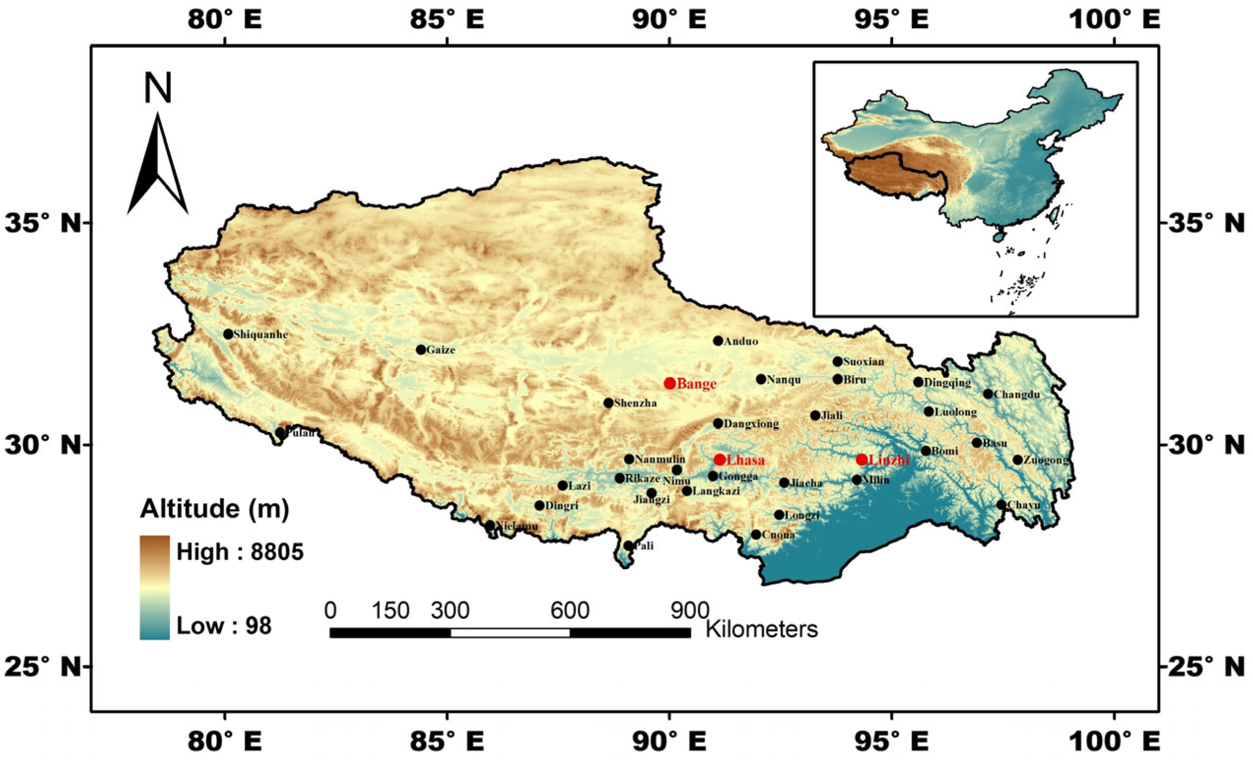
Figure 1. Distribution of weather stations over the TP. The black dots represent weather stations, and the red dots represent three stations with complete data required for calibration of the FAO56-PM model.
Applsci 15 12449 g001
Figure 2. Errors in ET0 arising from the recommended formula for Rs. (Rs was calculated using Fs while Rnl was measured. The error in Rn was caused solely by the estimated Rs).
Applsci 15 12449 g002
Figure 3. Errors in ET0 arising from the recommended formula for Rnl. (Rnl was calculated using Fnl while Rs was measured. The error in Rn was caused solely by the estimated Rnl).
Applsci 15 12449 g003
Figure 4. The original FAO56-PM for estimating ET0. Errors in ET0 arising from the recommended formulas for both Rs and Rnl. (Rs and Rnl were calculated using Fs and Fnl, respectively, see Figure 2 and Figure 3. The error in Rn was caused by both the estimated Rs and the estimated Rnl).
Applsci 15 12449 g004
Figure 5. Mere calibration of the recommended formula for Rs in FAO56-PM. (Errors in ET0 arising from the calibrated Fs and the original Fnl).
Applsci 15 12449 g005
Figure 6. Mere calibration of the recommended formula for Rnl in FAO56-PM. (Errors in ET0 arising from the original Fs and the calibrated Fnl).
Applsci 15 12449 g006
Figure 7. Comprehensive calibration of the recommended formulas for both Rs and Rnl in FAO56-PM. (Errors in ET0 arising from the calibrated Fs and the calibrated Fnl).
Applsci 15 12449 g007
Figure 8. Performance of the general method. (Errors in ET0 arising from the Fs and Fnl with coefficients derived from the AllenR method).
Applsci 15 12449 g008
Figure 9. Spatial distribution of annual and monthly ET0 over the TP from 1991 to 2020. (The scale at the bottom of the figure is the indicator for monthly ET0, unit: mm).
Applsci 15 12449 g009
Figure 10. The relative errors arising from the other method: (a) AllenO, (b) AllenS, and (c) AllenL.
Applsci 15 12449 g010
Figure 11. Trend analyses of ET0 at Lhasa from 1994 to 2020 under different calculation methods for FAO56-PM. (AllenM is set as the standard method for comparison).
Applsci 15 12449 g011
Figure 12. The spatial distribution of trends in ET0 over the TP from 1991 to 2020. (a) Trends calculated using AllenR; (b) Error by AllenO; (c) Error by AllenS; and (d) Error by AllenL.
Applsci 15 12449 g012
Figure 13. Averaged daily Rs, Rnl and Rn at the three experimental sites.
Applsci 15 12449 g013
Figure 14. Errors of estimated Rs, Rnl, Rn and ET0 under different calculation methods.
Applsci 15 12449 g014
Table 1. Geographic characteristics for the experimental sites and weather stations.
StationLatitude/NLongitude/E Altitude/mExperimental Period/Recording Time
Lhasa29.6791.133648.920 October 1993 to 31 December 2020
Linzhi29.5994.252991.81 September 2015 to 31 December 2020
Bange31.3890.024700.01 August 2014 to 31 July 2015
Shiquanhe32.5080.084278.61 January 1991 to 31 December 2020
Gaize32.1584.424414.91 January 1991 to 31 December 2020
Anduo32.3591.104800.01 January 1991 to 31 December 2020
Nanqu31.4892.074507.01 January 1991 to 31 December 2020
Pulan30.2881.253900.01 January 1991 to 31 December 2020
Shenzha30.9588.634672.01 January 1991 to 31 December 2020
Dangxiong30.4891.104200.01 January 1991 to 31 December 2020
Lazi29.0887.604000.01 January 1991 to 31 December 2020
Nanmulin29.6889.104000.11 January 1991 to 31 December 2020
Rikaze29.2588.883836.01 January 1991 to 31 December 2020
Nimu29.4390.173809.41 January 1991 to 31 December 2020
Gongga29.3090.983555.31 January 1991 to 31 December 2020
Qongjie29.0391.683740.01 January 1991 to 31 December 2020
Zedang29.2591.773551.71 January 1991 to 31 December 2020
Nielamu28.1885.973810.01 January 1991 to 31 December 2020
Dingri28.6387.084300.01 January 1991 to 31 December 2020
Jiangzi28.9289.604040.01 January 1991 to 31 December 2020
Langkazi28.9790.404431.71 January 1991 to 31 December 2020
Cuona27.9891.954280.31 January 1991 to 31 December 2020
Longzi28.4292.473860.01 January 1991 to 31 December 2020
Pali27.7389.084300.01 January 1991 to 31 December 2020
Suoxian31.8893.784022.81 January 1991 to 31 December 2020
Biru31.4893.783940.01 January 1991 to 31 December 2020
Dingqing31.4295.603873.11 January 1991 to 31 December 2020
Leiwuqi31.2296.603810.01 January 1991 to 31 December 2020
Changdu31.1597.173306.01 January 1991 to 31 December 2020
Jiali30.6793.284488.81 January 1991 to 31 December 2020
Luolong30.7595.833640.01 January 1991 to 31 December 2020
Bomi29.8795.772736.01 January 1991 to 31 December 2020
Basu30.0596.923260.01 January 1991 to 31 December 2020
Jiacha29.1592.583260.01 January 1991 to 31 December 2020
Milin29.2294.222950.01 January 1991 to 31 December 2020
Zuogong29.6797.833780.01 January 1991 to 31 December 2020
Mangkang29.6898.603870.01 January 1991 to 31 December 2020
Chayu28.6597.472327.61 January 1991 to 31 December 2020
Table 2. Coefficients in the empirical formulas of Fs and Fnl under different calculation methods.
MethodSiteFsFnl
abcdef
AllenOAll stations0.2500.5000.3400.1401.3500.350
Lhasa0.2800.5000.3400.1401.3500.350
AllenSLinzhi0.3040.4710.3400.1401.3500.350
Bange0.3040.5630.3400.1401.3500.350
Lhasa0.2500.5000.6300.2960.673−0.149
AllenLLinzhi0.2500.5000.2800.0760.997−0.324
Bange0.2500.500
500
0.8460.3450.507−0.054
Lhasa0.2800.5000.6300.2960.673−0.149
AllenCLinzhi0.3040.4710.2800.0760.997−0.324
Bange0.3040.5630.8460.3450.507−0.054
Lhasa0.2530.5560.5820.2640.721−0.149
AllenRLinzhi0.2580.5300.5820.2640.721−0.149
Bange0.2380.5980.5820.2640.721−0.149
Disclaimer/Publisher’s Note: The statements, opinions and data contained in all publications are solely those of the individual author(s) and contributor(s) and not of MDPI and/or the editor(s). MDPI and/or the editor(s) disclaim responsibility for any injury to people or property resulting from any ideas, methods, instructions or products referred to in the content.