Data-Driven Planning Phase of Maritime SAR Using Satellite Observations

Abstract

Maritime search and rescue operations rely on accurate drift predictions to define effective search areas for missing persons. Existing systems often depict uncertainty using statistical ellipses or ensemble-based probability maps, which may not effectively capture directional biases and underlying flow structures. In this study, we introduce a geometric framework that constructs possible object trajectories directly from the drift dynamics. Starting from the last known position, we integrate the translational and rotational drift components with arbitrary perturbations to model realistic scenarios. The resulting envelope of the trajectories defines a reachable set that adapts to the flow without relying on sampling or covariance estimations. Using satellite-derived wind and current data, we demonstrat that this approach produces envelopes that are physically consistent and operationally relevant. Our method offers a mathematically grounded alternative to ensemble techniques, enhancing interpretability and improving the SAR planning efficiency. We illustrate its effectiveness with examples that simulate real-world scenarios.

1. Introduction

Approximately two-thirds of the Earth’s surface is covered by water. Search and rescue (SAR) operations at sea are significantly challenged by the vast and dynamic nature of the maritime environment. When an object is lost, rescue teams strive to maximize the probability of detection while minimizing the time and resources required to locate it. Effective planning hinges on several key elements, notably the last known position, drift prediction, and object type. These factors collectively form the foundation for developing efficient and timely emergency response strategies [1].

The last known position is the initial point of reference used to plot the search area. This position provides the baseline from which SAR operations commence, allowing teams to establish a starting point for the search grid [1]. Drift prediction involves predicting the movement of an object over time owing to currents, wind, and other environmental factors [2]. Wind data are commonly obtained from satellite observations, whereas current speed and direction are often estimated from tide gauges and other oceanographic measurements [3]. Information on the size, buoyancy, and behavior of an object in water is critical for tailoring search operations. The type of object affects its interaction with environmental conditions, such as wind and waves, influencing drift patterns and search strategies [4,5].

Drift prediction models play a vital role in SAR operations by factoring in the effects of changing environmental conditions to forecast the potential destinations of drifting objects [2]. Research has highlighted the complex interplay between surface winds, waves, and ocean currents in determining the movement of floating debris in the ocean [6]. To accurately capture this complexity, advanced prediction methods are required to consider the combined effects of various environmental factors. Recent advancements have enhanced these methods by employing intelligent decision algorithms that leverage environmental indices and historical data [6,7]. These optimization techniques not only improve the precision and reliability of drift predictions but also increase operational efficiency by reducing the time required to locate targets [8].

In this study, we develop a geometric framework for predicting drift in maritime SAR operations, directly linking environmental forces with the possible paths of a drifting object. This approach uses satellite-derived wind and current data, along with local disturbances integrated into ocean models to characterize drift dynamics. It considers both translational and rotational elements, allowing the model to simulate realistic motion patterns under complex flow conditions. The collection of all potential endpoints at a specific forecast time forms the reachable set, which is a search boundary that naturally aligns with the flow structure and reflects its anisotropy and directional tendencies. This depiction highlights areas with the highest probability of object presence, aiding rescue teams in allocating resources more efficiently. Unlike statistical or ensemble-based techniques, the proposed method derives the search area directly from the governing dynamics, ensuring physical consistency and enhancing interpretability and operational effectiveness.

In this study, we define three essential terms with precise meanings. The drift trajectory describes the path taken by a floating object influenced by wind, currents, and other environmental factors. The reachable set includes all potential locations that an object might occupy after a specified forecast period, accounting for uncertainties in environmental conditions and possible variations in movement. The search envelope is the outer boundary of this set, providing a practical geometric depiction of the area in which the object is most likely to be located. These concepts collectively link the mathematical formulation of drift dynamics with its practical application in search-and-rescue operations.

Our framework integrates satellite data with a mathematical model that is analytically manageable and operationally significant. By deriving explicit equations for object trajectories that incorporate both translational and rotational drift components, the model accurately reflects the behaviors observed in maritime environments. The endpoints of these trajectories at a given forecast time determine a coherent and physically consistent size for the search envelope. This deterministic approach minimizes the need for sampling or covariance estimation, offering a clear alternative to purely statistical and heuristic approaches. Consequently, the proposed model serves as a dependable and interpretable tool for estimating search areas in real-world SAR planning scenarios.

2. Formulating the Drift of the Object

In a calm sea, where wind, waves, and surface currents are absent, a floating object is influenced mainly by two vertical forces: gravity and buoyancy. Gravity acts on the object’s mass and pulls it downward toward the Earth’s center [9]. Buoyancy, produced by the water displacement, exerts an upward force equal to the weight of the displaced fluid, following Archimedes’ principle [10]. When the density of the object is lower than that of water, the buoyant force balances or exceeds gravity, allowing the object to remain afloat [11].

The equilibrium between these two forces determines whether an object remains on the surface or becomes stably submerged [12]. In the vertical direction, the total force can be expressed as

$$\sum F_{\mathrm{vertical}}=mg-{\rho }_{\mathrm{w}}g{V}_{\mathrm{disp}}=0,$$

(1)

where m is the object mass, g is the gravitational acceleration, ${\rho }_{\mathrm{w}}$ is the water density, and $V_{\mathrm{disp}}$ is the displaced volume [13]. This force balance condition ensures flotation without vertical motion.

In realistic maritime environments, the forces acting on floating objects extend beyond gravity and buoyancy. Wind, wave-induced drift, and depth-dependent currents exert significant horizontal forces [14,15,16], whereas seasonal variability, sea surface temperature, salinity, and other environmental factors further influence drift [17].

The horizontal motion of a floating object is governed by Newton’s second law, that is

$$m{\displaystyle \frac{d\mathbf{v}}{dt}}=\sum {\mathbf{F}}_{\mathrm{horizontal}}.$$

(2)

In calm conditions, when horizontal forces are absent, we have

$$\sum {\mathbf{F}}_{\mathrm{horizontal}}=0,$$

(3)

which implies

$${\displaystyle \frac{d\mathbf{v}}{dt}}=0\Rightarrow \mathbf{v}\left(t\right)={\mathbf{v}}_0.$$

(4)

This means that if the object is initially at rest, ${\mathbf{v}}_0=\mathbf{0}$, it remains stationary; otherwise, it retains its initial velocity relative to the water surface.

Under realistic conditions, horizontal forces act on an object, causing it to drift. The position of the object at time t, denoted by $r\left(t\right)$, is approximated as the time integral of the total drift velocity, as follows [18]

$$r\left(t\right)=r\left(0\right)+{\int }_0^t{\mathbf{V}}_{\mathrm{tot}}(r\left(s\right),s)ds,$$

(5)

where $r\left(0\right)$ is the last known position, which is considered as the initial position in the approximation formula, and the total drift velocity decomposes as

$${\mathbf{V}}_{\mathrm{tot}}(r\left(t\right),t)={\mathbf{V}}_{\mathrm{curr}}(r\left(t\right),t)+{\mathbf{V}}_{\mathrm{lee}}\left(t\right),$$

(6)

where ${\mathbf{V}}_{\mathrm{curr}}$ denotes the current-induced drift and ${\mathbf{V}}_{\mathrm{lee}}$ represents the leeway drift caused by wind and waves. In SAR practice, the wave contribution is typically included within the leeway drift (see Section Leeway Models for further details).

Operational SAR systems address drift uncertainty by employing an ensemble, which is a collection of multiple drift simulations designed to represent the uncertainty in the predicted trajectory of a drifting object. Each simulated trajectory is an ensemble member, and together, they provide a probabilistic description of drift prediction. Thus, the envelope, which determines the search area, is the closed curve (or region) formed by the endpoints or positions at a given time T of all ensemble trajectories. It delineates the outermost extent of possible object locations given the ensemble [3].

A common method used is the ellipse envelope. It grows over time in the main direction of movement. The long side of the ellipse shows changes caused by the wind. The short side shows spreading due to waves and currents. Search teams usually start from the center of the ellipse. But this method assumes the same level of uncertainty everywhere and does not consider directional errors. This can make it less accurate in complex conditions [19]. Another method is the ensemble-derived envelope. It is made from a group of changed paths. This method creates a map showing where an object might be. It shows both areas where paths gather and the less likely outer areas [3].

Leeway Models

A leeway model is a mathematical or empirical tool used in maritime SAR to predict the wind-induced drift of objects or people in water. This occurs when the wind pushes an object off its intended or natural path, causing it to move downwind. Leeway models are critical for estimating the drift paths of search objects. The process varies depending on whether the object is a person, vessel, or debris [20,21,22]. In particular, incorporating wave-induced effects, such as Stokes drift, into trajectory forecasts has been shown to significantly improve the accuracy of surface drifter predictions [23]. For some floating objects, wind-induced drift may dominate; however, including the Stokes drift can still refine the predictions and enhance SAR performance [24]. Leeway drift, ${\mathbf{V}}_{\mathrm{lee}}=\alpha {\mathbf{V}}_{\mathrm{wind}}$, is typically calculated using empirical formulas, field observations, or tracking methods. Here, $\alpha$ is the leeway coefficient, which depends on factors such as the object’s geometry, exposure to wind, and environmental conditions, and may vary from $0.5\%$ to $3\%$.

In practice, the dominant forces driving drift are the total water current and wind-driven leeway, whereas the wave-induced Stokes drift is comparatively small and effectively absorbed into the leeway model. Directly modeling wave effects requires detailed knowledge of the sea state and object properties, adding unnecessary complexity and uncertainty to the operational SAR. Therefore, SAR models emphasize the most significant and predictable drift components to ensure reliable and timely forecasts [25].

3. The Proposed Geometric Approach

Uncertainty is an inherent aspect of drift prediction in maritime SAR, reflecting the variability and limited predictability of the object trajectories. It arises from multiple sources, including measurement errors, unforeseen environmental changes, and the intrinsic complexity of ocean dynamics [3].

In SAR operations, the last known position, denoted by P, marks the most recent verified location of an object, which is obtained from sightings, communications, or tracking devices. From this reference point, operational models predict the object’s drift using environmental forcing fields, such as wind, waves, and currents. Because these fields and the object’s leeway contain uncertainties, SAR systems do not rely on a single trajectory. Instead, they generated an ensemble of trajectories by slightly varying the drift inputs. The endpoints of these trajectories at a given forecast time form a cloud of possible positions, from which an envelope—often represented as an ellipse—is constructed to guide search planning. The self-motion of survivors is not modeled explicitly but is indirectly included in the overall size of this envelope [3]. Thus, during the planning phase of a SAR mission, the central objective is to obtain the best possible approximation of this envelope.

In our approach, we adopted the same total drift vector as in the literature, ${\mathbf{V}}_{\mathrm{tot}}(r\left(t\right),t)$, to represent the combined influence of the wind, currents, and waves. Smaller-scale perturbations and environmental irregularities are difficult to capture explicitly. Thus, we assume that the object has an inherent tendency to move in arbitrary directions, whereas the dominant drift governs its motion. The resulting trajectory can thus be interpreted as the path shaped by the total drift acting on the underlying perturbations. Thus, driving from Equation (5), we obtain ${\displaystyle \frac{dr}{dt}}=\dot{r}\left(t\right)={\mathbf{V}}_{\mathrm{tot}}(r\left(t\right),t)$. To consider the uncertainty in motion, we added a unitary vector v that points in any direction, leading to the following drift equation:

$${\displaystyle \frac{dr}{dt}}={\mathbf{V}}_{\mathrm{tot}}(r\left(t\right),t)+v,$$

(7)

This equation is consistent with the formulation given in [24], where a random perturbation is added to the drift equation. The unit vector v introduced in Equation (7) represents a small and unpredictable component of motion that is always present in real maritime environments. This term captures several sources of variability in a unified manner: (i) local turbulence and unresolved eddies that slightly deviate the object from the dominant drift direction; (ii) observational uncertainty in the last known position or in the environmental data; and (iii) possible self-motion of survivors or floating objects caused by intentional swimming or wave impact. By including all these effects within a single geometric term, the model retains a simple analytical while representing the realistic range of deviations that occur in practice. This approach allows the reachable set to adapt naturally to both environmental fluctuations and human or object behavior, resulting in a physically consistent and operationally meaningful description of uncertainty in drift prediction.

Now, solving the obtained differential equation in Equation Using (7), we estimate the ensemble envelope at a given time T as follows:

$$\mathcal{E}\left(T\right)=\left\{r\left(T\right):\dot{r}\left(t\right)={\mathbf{V}}_{\mathrm{tot}}(r\left(t\right),t)+v,r\left(0\right)=P,\right\},$$

(8)

where $r\left(0\right)=P$ is the last known position of the object, which is considered the initial point in our approximation. We remind that v is a unitary vector in all directions. Starting from the last known position, $r\left(0\right)$, relation (8) provides the ensemble set as the set of endpoints of a family of admissible trajectories whose velocities are given by the total drift vector plus a unit vector in arbitrary directions at a forecast time T.

The following are some of the advantages of our approach: (1) Unlike a statistical ellipse, this construction does not depend on sampling or covariance estimation but is derived directly from the dynamics of the drift field. (2) The method provides a mathematically rigorous framework that captures anisotropy and directional bias transparently. (3) It complements existing ensemble-based approaches and offers the potential to yield search areas that are both physically consistent and informative.

Next, we propose a possible form of the total drift vector based on our observations of satellite imagery of the currents and wind. Then, we use it to solve the differential equation in Equation (8) to present the equation of the envelope of the ensemble, addressing the SAR problem, as follows:

3.1. The Proposed Classification for the Total Drift Vector

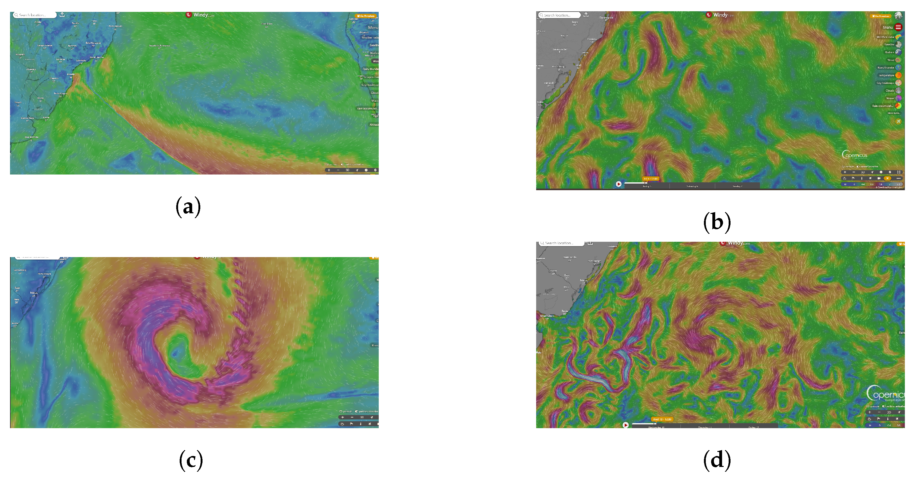
We first note that the most influential factors in the trajectory of the lost object are the current and wind. As illustrated in Figure 1, which are based on satellite imagery, the SAR operation region can be discretized into sub-regions where either translational and/or rotational vector fields reasonably approximate currents and wind.

Therefore, in our proposed approach, we model the total drift vector as the superposition of translational and rotational vectors, expressed as follows: where $r\left(t\right)=\left(x\right(t),y(t\left)\right)$ denotes the position of the object at time t.

$${\mathbf{V}}_{\mathrm{tot}}(x\left(t\right),y\left(t\right),t)=(a\left(t\right),b\left(t\right))+c\left(t\right)(-y\left(t\right),x\left(t\right)).$$

(9)

One observes that $\left(a\right(t),b(t\left)\right)$ in Equation (9) represents the translational drift, whereas $c\left(t\right)(-y(t),x(t\left)\right)$ corresponds to the rotational drift at time t, where $c\left(t\right)$ denotes the scalar angular intensity of rotation. The translational component models situations in which an object is passively transported along a dominant flow direction, such as currents or steady winds, whereas the rotational component captures drift patterns governed by vortical winds or circular currents. When $c\left(t\right)=0$, the drift reduces to pure translation, and when $a\left(t\right)=b\left(t\right)=0$, the drift reduces to pure rotation. This formulation has two main advantages: (1) it captures realistic scenarios by combining uniform displacement with rotational motion, and (2) it provides a tractable mathematical framework for deriving trajectories.

Parameterization from Satellite-Derived Data

The coefficients $a\left(t\right)$, $b\left(t\right)$, and $c\left(t\right)$ in Equation (9) are obtained directly from satellite-derived wind and current fields such as those available on www.windy.com, which combines data from the ECMWF and Copernicus ocean models. For each time t, the translational components $a\left(t\right)$ and $b\left(t\right)$ correspond to the horizontal velocity of the total drift in the Cartesian coordinates. If the wind or current at time t has magnitude $V\left(t\right)$ (in km/h) and direction $\theta \left(t\right)$ measured counterclockwise from the east, then

$$\left(a\right(t),b(t\left)\right)=V\left(t\right)(cos\theta (t),sin\theta (t\left)\right).$$

For example, a wind of $7\mathrm{km}/\mathrm{h}$ toward the southeast ($\theta ={45}^{\circ }$) is represented as $(a,b)=(7cos{45}^{\circ },7sin{45}^{\circ })$. When both wind and current data are available, their effects are combined by simple vector superposition, yielding the total translational drift at that time.

The rotational coefficient $c\left(t\right)$ represents the local angular intensity of rotation of the drift field. In practice, it may be estimated from the curvature of the streamlines or from the differences in the directions of the neighboring velocity vectors in the satellite imagery. A positive value of $c\left(t\right)$ corresponds to counterclockwise rotation, whereas a negative value indicates a clockwise motion.

This procedure creates a simple and intuitive connection between the satellite information and The parameters used in Equation (9).

3.2. The Trajectory Formulation

Although the wind and current vectors may vary several times over the time interval $[0,T]$, and thus the total drift also changes repeatedly, this interval can be subdivided into n sub-intervals $[t_i,t_{i+1}]$, $i=1,\dots ,n$, with $t_1=0$ and $t_{n+1}=T$, such that the wind and current vectors remain approximately constant within each sub-interval. The subdivision of the total forecast period into sub-intervals is directly related to the time variation in parameters $a\left(t\right)$, $b\left(t\right)$, and $c\left(t\right)$. In realistic maritime conditions, these parameters—representing the translational and rotational drift components—remain approximately constant for certain time spans and change only when the Environmental forcing fields vary noticeably. Instead of introducing explicit time-dependent variables into Equation (9), which would increase analytical complexity and accumulate numerical errors, we divide the total interval $[0,T]$ into smaller sub-intervals $[t_i,t_{i+1}]$. Within each sub-interval, the parameters are treated as constant, allowing the model to reflect gradual temporal changes in the environment while maintaining a simple and stable formulation.

According to Equation (9), the total drift in the ith sub-interval $[t_i,t_{i+1}]$ can then be modeled as

$$V^i(x\left(t\right),y\left(t\right),t)=(a_i,b_i)+c_i(-y\left(t\right),x\left(t\right)).$$

Let $(p_1^i,p_2^i)$ denote the initial position of the drifting object—latitude $p_1^i$ and longitude $p_2^i$—at time $t_i$, which represents the last known position for the sub-interval $[t_i,t_{i+1}]$. Following Equation (7), we use the vector $v=(v_1,v_2)$ to represent the uncertainty. In this case, however, we take the direction corresponding to the path along which the object arrives at the position $(p_1^i,p_2^i)$. This vector specifies the direction in which the object is presumed to move at the beginning of the subinterval.

Therefore, the trajectory of the object in the ith sub-interval is given by

$$\begin{array}{c}\hfill r_i\left(t\right)=(x_i\left(t\right),y_i\left(t\right)),\&\left\{\begin{array}{c}{x}_i\left(t\right)=a_{i}t+cos\left(c_{i}t\right)(p_1^i+t{v}_1)-sin\left(c_{i}t\right)(p_2^i+t{v}_2),\hfill \\ y_i\left(t\right)=b_{i}t+sin\left(c_{i}t\right)(p_1^i+t{v}_1)+cos\left(c_{i}t\right)(p_2^i+t{v}_2).\hfill \end{array}\right.\end{array}$$

(10)

Indeed, it is straightforward to verify that the initial velocity of the curve

$$r_i\left(t\right)=(x_i\left(t\right),y_i\left(t\right)),t\in [0,t_{i+1}-t_i]$$

is the vector

$$(a_i,b_i)+c_i(-p_2^i,p_1^i)+(v_1,v_2),$$

and its initial point is $(p_1^i,p_2^i)$. These satisfy the required conditions for a trajectory, as stated in Equation (8). Finally, by shifting the time t to $t+t_i$, we obtain the solutions in (10).

Equation (10) represents a spiral-like trajectory, combining circular motion (due to rotation) and directional drift (due to $(a,b)$). The ensemble envelope after time T is obtained by combining all trajectories $r_i\left(t\right)$ whose initial velocity is given by $V^i+v$, where v is fixed for each specific trajectory and whose initial point is $(p_1^i,p_2^i)$. That is, reminding that $t_1=0$ and $t_{n+1}=T$, the trajectory of the object from time 0 to T is equal to

$$r\left(t\right)=\left\{\begin{array}{cc}{r}_1\left(t\right),\hfill & \mathrm{if}t\in [0,t_2],\hfill \\ ⋮\hfill & \\ r_i\left(t\right),\hfill & \mathrm{if}t\in [t_i,t_{i+1}],\hfill \\ ⋮\hfill & \\ r_n\left(t\right),\hfill & \mathrm{if}t\in [t_n,t_{n+1}].\hfill \end{array}\right.$$

Algorithm 1 provides the steps of providing the drift trajectories and ensemble envelope.

Algorithm 1 Computation of Drift Trajectories and Ensemble Envelope

Require: Last known positions $\{p^i=(p_1^i,p_2^i)\}$ at times $\left\{t_i\right\}$, total time T, number of subintervals n, and drift parameters $\left\{(a_i,b_i,c_i)\right\}$ for each $[t_i,t_{i+1}]$.

Ensure: Local trajectories $\left\{r_i\left(t\right)\right\}$ on each $[t_i,t_{i+1}]$ and ensemble envelope at time T.

1: Partition $[0,T]$ into subintervals $[t_i,t_{i+1}]$, $i=1,\dots ,n$, with $t_1=0$ and $t_{n+1}=T$. 2: for$i=1$do 3:   Define the local drift field: $$V^1(x,y)=(a_1,b_1)+c_1(-y,x),$$ where $(a_1,b_1)$ and $c_1$ represent the translational and rotational drifts on $[0,t_2]$. 4:   Choose directions $\{v^1,\dots ,v^m\}\subset S^1$ such that $\angle (v^j,v^{j+1})=\frac{2\pi }{m}$, where $S^1$ denotes the unit circle. 5:   Compute trajectories for $t\in [0,t_2]$: $$r_j^1\left(t\right)=(a_1,b_1)t+R_{c_{1}t}(p^1+t{v}^j),R_{c_{1}t}=\left(\begin{array}{cc}cos\left(c_{1}t\right)& -sin\left(c_{1}t\right)\\ sin\left(c_{1}t\right)& cos\left(c_{1}t\right)\end{array}\right),$$ where $p^1$ is the last known position at $t=0$. 6:   The ensemble envelope at time $t_2$ is given by $$\mathcal{E}\left(t_2\right)=\left\{r_j^1\left(t_2\right):{\dot{r}}_j^1\left(0\right)=V^1+v^j,r_j^1\left(0\right)=p^1\right\}.$$ 7: end for 8: for$i=2$to n do 9:   Define the local drift field: $$V^i(x,y)=(a_i,b_i)+c_i(-y,x),$$ where $(a_i,b_i)$ and $c_i$ correspond to the translational and rotational drift on $[t_i,t_{i+1}]$. 10:   for$j=1$to m do 11:     For each $p_j^i=r_j^{i-1}\left(t_i\right)$ and direction $v^j={\dot{r}}_j^{i-1}\left(0\right)-V^i$, compute $$r_j^i\left(t\right)=(a_i,b_i)t+R_{c_{i}t}(p_j^i+t{v}^j),R_{c_{i}t}=\left(\begin{array}{cc}cos\left(c_{i}t\right)& -sin\left(c_{i}t\right)\\ sin\left(c_{i}t\right)& cos\left(c_{i}t\right)\end{array}\right),t\in [0,t_{i+1}].$$ 12:     Shift local time to the global reference: $t\leftarrow t_i+t$. 13:   end for 14:   The ensemble envelope at time $t_{i+1}$ is $$\mathcal{E}\left(t_{i+1}\right)=\left\{r_j^i\left(t_{i+1}\right):{\dot{r}}_j^i\left(t_i\right)=V^i+v^j,r_j^i\left(t_i\right)=p_j^i\right\}.$$ 15: end for 16: Assemble global trajectories: concatenate local segments $\left\{r_j^i\left(t\right)\right\}$ across all intervals to form global trajectories for each directional realization $v_j$. 16: Compute ensemble envelope at time T: collect all end positions $\left\{r_j\left(T\right)\right\}$ and determine the global envelope, as $$\mathcal{E}\left(T\right)=\left\{r_j^n\left(T\right):{\dot{r}}_j^i\left(t_i\right)=V^n+v^j,r_j^n\left(t_n\right)=p_j^n\right\}.$$

Example 1.

Maritime SAR under time-varying wind and current conditions.

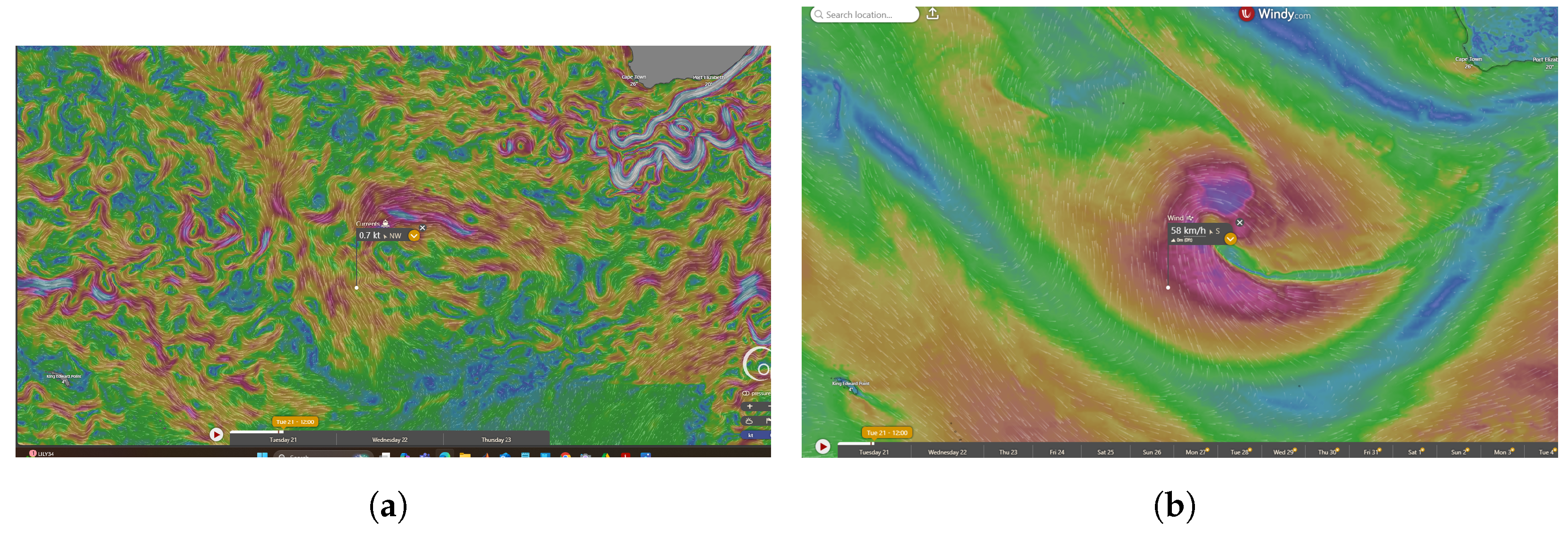
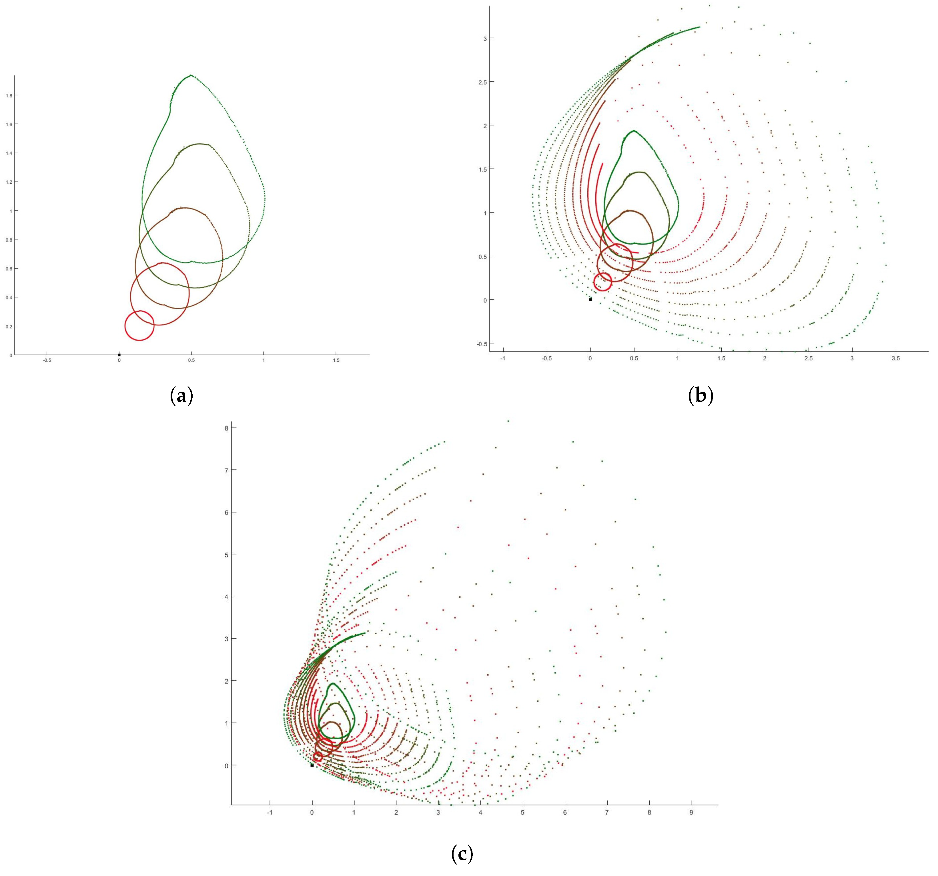
In this example, we simulated a SAR operation in which a drifting object was tracked after its last known position of ${48}^{\circ }{57}^{\prime }{3}^{″}\mathrm{S},8^{\circ }{20}^{\prime }{0}^{″}\mathrm{W}$, as indicated by the flag marker in the maps below, Figure 2. The rescue team integrated satellite-derived wind and current fields to reconstruct possible trajectories and predict the evolving reachable set of the object over three consecutive time intervals. The possible locations of the object after each hour are shown with closed curves.

In the first stage (Figure 3a), the wind field is relatively steady however strong with the velocity of $58km/h$, producing a set of possible trajectories centered near the last known position. The motion was mainly translational, and the uncertainty region remained small, first in the northwest direction and then in the north.

During the second stage (Figure 3b), the environmental forcing intensifies, causing a deformation of the envelope and the emergence of rotational patterns in the drift field. Over the course of nine hours, the reachable set elongates in all directions, and the object may even return to its initial position.

In the third stage (Figure 3c), a marked change in total force direction produces a shear effect, broadening the uncertainty region and generating anisotropy in the predicted search area. This asymmetry indicates a higher probability of finding an object along the direction of the newly dominant current.

This case study highlights the role of geometric and systematic analyses in improving maritime SAR planning. By interpreting the evolution of the reachable sets through a geometric framework, rescue teams can evaluate how environmental forces shape the admissible trajectories of drifting objects. The envelopes obtained from our formulation provide a structured and physically grounded representation of uncertainty, allowing for the systematic delineation of the most probable regions of object presence. This geometric perspective complements operational decision-making by translating complex wind–current interactions into interpretable spatial patterns, thereby enhancing SAR planning efficiency and precision.

Comparison with traditional methods. Traditional search-area estimation methods often employ an elliptical envelope or a Monte Carlo ensemble approach. The elliptical method summarizes uncertainty by fitting an expanding ellipse aligned with the mean drift direction. Although this representation is simple and operationally convenient, it assumes uniform variability and does not capture directional asymmetries or rotational effects produced by complex wind and current interactions.

Monte Carlo ensemble techniques improve on this by generating a large number of perturbed trajectories and constructing a probability field of possible object positions [26]. This stochastic approach can reproduce variability, but it depends on repeated random sampling and is computationally expensive for real-time application.

The proposed geometric framework offers a deterministic solution. By deriving the reachable set directly from the drift equation, it produces a physically consistent envelope that reflects anisotropy and rotational deformation without relying on statistical fitting or random ensembles. This provides the same interpretive value as traditional methods while maintaining analytical simplicity and high computational efficiency, making it suitable for operational SAR applications.

Comparison with Operational Drift Models. To assess the practical relevance of the proposed geometric framework, To demonstrate the practical relevance of the proposed geometric framework, we compared its predicted envelopes conceptually with the results generated by OpenDrift, an operational open-source system widely used for maritime drift prediction [24,25]. Both approaches employ the total drift field ${\mathbf{V}}_{\mathrm{tot}}={\mathbf{V}}_{\mathrm{curr}}+{\mathbf{V}}_{\mathrm{lee}}$ under perturbed wind and current conditions. In OpenDrift, the uncertainty of drift prediction is obtained statistically from an ensemble of perturbed trajectories, resulting in a probability density map or elliptical search region. In contrast, our framework computes the reachable set analytically from

$$\dot{r}\left(t\right)={\mathbf{V}}_{\mathrm{tot}}(r\left(t\right),t)+v,\left|\right|v\left|\right|=1,$$

(11)

and defines the envelope $\mathcal{E}\left(T\right)$ analytically, without requiring Monte Carlo sampling. When both methods are applied under comparable environmental conditions (e.g., wind and current fields obtained from satellite observations), the geometric envelope naturally reproduces the qualitative extent and orientation of the ensemble cloud obtained by OpenDrift. Moreover, the proposed framework explicitly captures anisotropic deformation and rotational drift effects, which are not readily represented by the statistical ellipses. Therefore, the geometric reachable set model provides a mathematically rigorous and computationally efficient alternative that remains consistent with operational drift patterns and supports real-time SAR planning.

4. Conclusions and Discussion

In this study, we propose a geometric framework for estimating search areas in maritime SAR operations, grounded in the concept of reachable sets of admissible trajectories. By integrating translational and rotational drift components with arbitrary perturbations, the framework captures anisotropic and directionally biased motion patterns that are often inadequately represented by traditional statistical ellipses. Unlike sampling-based methods, the proposed construction derives the search envelopes directly from the underlying drift dynamics, thereby providing a deterministic and physically consistent representation of the uncertainty.

The incorporation of satellite-derived wind and current fields enables the operational implementation of this geometric model, allowing for the dynamic adjustment of search areas as environmental conditions evolve. This systematic approach provides a mathematically rigorous and computationally efficient alternative to ensemble-based techniques, with the potential to enhance the accuracy and timeliness of rescue planning.

Although comprehensive validation against real SAR incidents is left for future work, the present results demonstrate the theoretical soundness and practical promise of this method. The example implemented in the MATLAB environment illustrates how the proposed framework can be used to simulate drift trajectories, construct envelopes, and visualize evolving search regions in a coherent geometric form. Future developments will focus on data assimilation, uncertainty quantification, and real-time integration with operational SAR systems to further extend the model’s applicability.

Influence of object-specific leeway coefficients. In practical SAR operations, the total drift velocity is commonly expressed as

$${\mathbf{V}}_{\mathrm{tot}}={\mathbf{V}}_{\mathrm{curr}}+\alpha {\mathbf{V}}_{\mathrm{lee}},$$

where ${\mathbf{V}}_{\mathrm{curr}}$ represents the ambient surface current and $\alpha$ is the leeway coefficient. The leeway coefficient depends on the object’s geometry, buoyancy, and exposure to wind. Different objects therefore experience distinct effective drifts even under identical environmental conditions. Within the proposed framework, this variability is naturally captured by assigning a specific value of $\alpha$ to each object type. This results in in different drift trajectories, ensemble sets, and the reachable envelopes. This formulation allows the model to adapt to diverse operational scenarios while preserving analytical simplicity and computational efficiency.

Scope, limitations, and future developments. The efficacy of the proposed geometric framework is contingent on the quality and resolution of the environmental data used to parameterize the drift field. Satellite-derived wind and current products are generally available at spatial resolutions of several kilometers and temporal intervals of several hours. Therefore, small-scale variations and rapid changes in nearshore or highly nonlinear flow conditions may not be comprehensively represented. In such regions, local effects, including wave–current interactions, tides, and coastal geometry, can introduce additional deviations in the drift that extend beyond the scope of the current formulation. Nevertheless, these limitations are primarily associated with data availability rather than the model structure itself. As high-resolution and near-real-time satellite observations become accessible, the proposed framework can be readily adapted to incorporate these inputs. Future developments will focus on integrating the geometric model with operational SAR platforms to facilitate real-time updates of the reachable set. This will provide a practical bridge between mathematical modeling and decision-making in maritime SAR operations.

Remark on the geostrophic effect. In this study, the geostrophic component of ocean circulation was not explicitly incorporated into the drift formulation. The model focuses on short- to medium-term periods. During these times, surface movement is mainly affected by wind and near-surface currents, as seen in satellite data. For extended prediction horizons or large-scale applications, a geostrophic velocity term, ${\mathbf{V}}_{\mathrm{geo}}$, may be integrated into the total drift field in future iterations of the model.