Article

Research on MPC Path-Tracking Control Algorithm Based on the Generalized-Dynamics Model of “Steering Robot-Controlled Vehicle”

1
Institute of Automotive Engineering, Jiangsu University, Zhenjiang 212013, China
2
Shenyang Shenda Connected Vehicle Collaborative Innovation Center Co., Ltd., Shenyang 110044, China
*
Author to whom correspondence should be addressed.
Appl. Sci. 2025, 15(22), 12245; https://doi.org/10.3390/app152212245
Submission received: 9 October 2025 / Revised: 9 November 2025 / Accepted: 15 November 2025 / Published: 18 November 2025

Featured Application

The findings of this paper lay the groundwork for incorporating MPC-related research into driving robots in the future.

Abstract

We propose an integrated model predictive control (MPC) scheme for steering-robot path tracking that directly optimizes the robot voltage and embeds steering-angle limits as linear-inequality voltage constraints inside the optimizer. This avoids cascade-induced error accumulation and extra phase lag in MPC+PID while guaranteeing actuator-level feasibility. A Simulink–CarSim co-simulation evaluates two scenarios: (1) double-lane change (DLC) at 70/40 km·h−1; and (2) straight-line tracking with/without sinusoidal crosswind modeled as an equivalent lateral force. Metrics include lateral-error RMS/Peak/P95 and real-time statistics (WCET, average per-update time, and utilization rate). The results show consistent gains: at 70 km·h−1, RMS/Peak/P95 decrease by 22.3%/18.0%/17.7%; and, at 40 km·h−1, by 17.0%/19.5%/18.9%. Real-time feasibility is met with T = 10 ms, average ≈ 1.7 ms, WCET ≈ 2.1~2.3 ms, utilization ratio ≈ 0.17. Under crosswind, robustness improves over the cascaded baseline by 9.7%/35.6%/30.8% on RMS/Peak/P95. The method provides tighter tracking, stronger disturbance rejection, and strict timing for safety-critical testing.

1. Introduction

Vehicle safety requirements continue to rise, and test scenarios are increasingly hazardous and diverse. Driving robots are therefore deployed to replace human drivers in tests to enhance repeatability and reduce risks under uncertain conditions. Among pedal, steering, and shift robots, this work focuses on steering robots for lateral control, whose direct performance is reflected by how accurately the vehicle follows a reference path.

1.1. Related Work

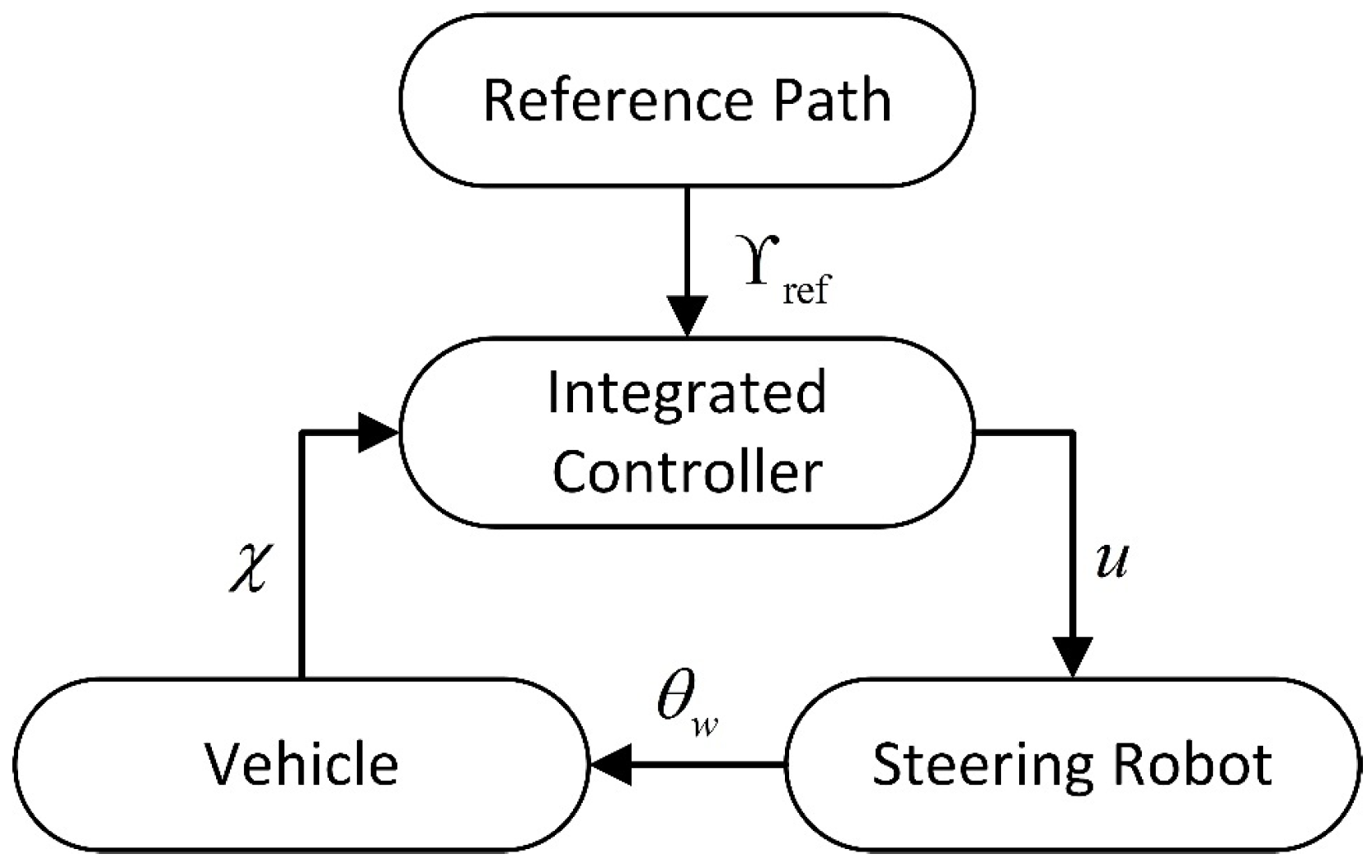
Most driving-robot solutions use a cascaded structure in which a path-tracking controller outputs a desired front-wheel angle, which is converted to a steering-wheel command and then tracked by a separate actuator loop [1,2,3,4,5,6]; see Figure 1. This separation may introduce phase lag and, more importantly, the inconsistent enforcement of physical steering limits across loops. Moreover, cascades are prone to multi-layer error accumulation: set-point conversion and actuator tracking errors all compound along the chain, eventually degrading the vehicle-level path accuracy.
MPC is widely used for vehicle path tracking owing to prediction and explicit constraints [7,8,9,10,11,12,13,14,15,16,17,18,19,20,21,22,23,24,25]. Prior studies often respect steering-angle bounds via post-saturation or anti-windup outside the optimizer, or model simplified steering dynamics while still commanding the angle rather than the robot’s voltage.

1.2. Novelty

Two gaps remain: (a) the lack of an integrated formulation that optimizes the steering-robot voltage directly, thereby preventing cascade-induced multi-layer error accumulation; and (b) the absence of linear-inequality mappings that embed physical steering-wheel angle bounds as voltage constraints within the optimizer, guaranteeing actuator-level feasibility without ad hoc post-saturation.
In contrast to cascaded designs, as shown in Figure 2, we propose an integrated MPC that directly optimizes the robot voltage and embeds steering-angle bounds as linear inequalities inside the QP, thereby avoiding cascade-induced multi-layer error accumulation and improving path-tracking accuracy.
Unlike passenger-carrying ADS, driving robots for vehicle testing operate unmanned on closed proving grounds and are intended to reproduce safety-critical scenarios. Consequently, constraint design should not include comfort margins; instead, it should be opened up to the vehicle’s physical limits while remaining mechanically feasible.

1.3. Contribution

  • Integrated formulation: A generalized vehicle-steering-robot model and an integrated MPC that uses the robot voltage as the control input, thereby avoiding cascade-induced multi-layer error accumulation;
  • Physically feasible constraints: Linear-inequality mappings that convert steering-wheel angle bounds into voltage constraints inside the optimizer, avoiding ad hoc post-saturation and ensuring actuator-level physical feasibility;
  • Path-tracking evaluation: Side-by-side comparisons against a cascaded MPC–PID baseline under identical conditions, using the vehicle-level criterion—lateral tracking error e y as the primary metric; we report RMS and peak e y over matched time windows.

2. Materials and Methods

2.1. Steering Robot Modeling

This section establishes the mathematical model of the steering robot.
Unlike pedal robots and gear-shifting robots, steering robots do not require actuators capable of linear displacement; they only need to achieve a rotational effect. Therefore, the structure of steering robots can be either a more complex structure that uses a universal joint to connect the motor to the mechanical arm and mechanical claws to grip the steering wheel [2], or a structure in which the motor is directly mounted on the steering wheel.
In order to facilitate the establishment of the mathematical model of the steering robot, the structure of the steering robot in this paper adopts the structure of DC motors directly mounted on the steering wheel, so that the output angle of the DC motors is equal to the steering wheel angle, and the mounting structure is shown in Figure 3.
The control model of a DC motor can be represented by the armature voltage balance equation, the electromagnetic torque balance equation, and the output torque balance equation, which are established separately as follows:
u = R i + k e ω + L d i d t ,
T e = k m i ,
T e = T L + B ω + J d ω d t ,
where:
u —the voltage across the armature;
R —the armature circuit resistance;
i —armature current;
k e —inverse electromotive force constant;
ω —the rotor angular velocity of the motor;
L —the armature circuit inductance;
T e —the electromagnetic torque;
k m —the electromagnetic torque constant;
T L —the load torque;
B —the motor damping factor;
J —the moment of inertia of the motor output shaft.
By associating Equation (2) with Equation (3), we can obtain the following:
d ω d t = k m i J T L J B ω J .
Neglecting the reactance voltage drop in the armature circuit due to changes in armature current, i.e., d i d t = 0 , Equation (1) can be deformed as follows:
i = 1 R ( u k e ω ) .
Substituting Equation (5) into Equation (4), the equation of state of the DC motor can be obtained as follows:
x ˙ 1 = x 2 x ˙ 2 = k m k e J R + B J x 2 + k m J R u T L J ,
where:
x 1 —the angle of rotation of the motor rotor;
x 2 —the angular speed of the motor rotor.
Based on the physical structure of the driving robot chosen in this paper, we can directly use the state equation of this DC motor as the state equation of the steering robot.
At this point, the modeling of the steering robot is complete.

2.2. Vehicle Transverse Two-Degree-of-Freedom Dynamics Model

In order to reduce the computation of the controller, we choose the vehicle two-degree-of-freedom dynamics model as the control model.
To establish the vehicle two-degree-of-freedom dynamics model, it is necessary to, first, analyze the force on the vehicle as a whole and establish the basic model, then analyze the lateral force on the vehicle and obtain the expression of lateral force, then obtain the relationship equation between the lateral deflection angle and each parameter through the two-degree-of-freedom bicycle model of the vehicle, and, finally, substituting these expressions into the basic model; then, we can obtain the lateral two-degree-of-freedom dynamics model.
We make the following assumptions to simplify the model:
(1) The force of the air on the vehicle will only affect motion in the x-axis of the body coordinate system; rotation in the y-axis and along the z-axis will not be affected by the air.
(2) The vehicle runs in a two-dimensional plane, i.e., no velocity in the z-axis.
(3) Vehicle tire forces act in a linear interval.
(4) The left/right wheels on each axle are lumped into a single front wheel and a single rear wheel; axle-level parameters are aggregated.
(5) Steering and sideslip angles are small so that standard linearization is used, e.g., tan δ δ ; kinematic couplings are linearized accordingly.
(6) Steering-system friction, backlash, and hysteresis are neglected.
(7) The vehicle body is modeled as a rigid body; suspension compliance, vertical tire dynamics, and load transfer are neglected.

2.2.1. Basic Modeling

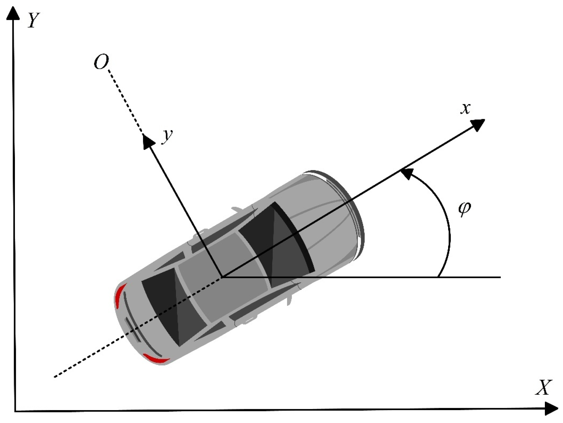
Establish the position relationship as shown in torque (Figure 4), where the x-axis and y-axis represent the global coordinate axes, the x-axis and y-axis represent the body coordinate axes, the x-direction is forward along the central axis of the vehicle, and the y-axis direction is a 90-degree counterclockwise rotation of the x-direction.
Decompose the planar motion of a vehicle into translation and rotation.
Analyze the process of vehicle translation:
Assuming that the vehicle is a mass, the force on the mass is analyzed according to Newton’s second law, which gives
m a y = F y f + F y r m a x = F x f + F x r F a e r o ,
where:
a y —the acceleration of the vehicle’s center of mass along the y-axis, a y = d 2 y d t 2 ;
F y f , F y r —the forces on the front and rear axles of the vehicle in the y-axis direction, respectively;
F x f , F x r —the forces on the front and rear axles of the vehicle in the x-axis direction, respectively;
F a e r o —the air resistance of the vehicle in the x-axis direction.
In the process of translation, a y is produced by the combined action of two accelerations. These two accelerations are the inertial acceleration y ¨ of the vehicle along the y-axis and the centripetal acceleration a c of the vehicle as it rotates around the rotation O :
a y = y ¨ + v x φ ˙ ,
a c = v x 2 R = v x φ ˙ .
Substituting Equation (8) into Equation (7) yields the following:
m y ¨ + v x φ ˙ = F y f + F y r .
Similarly, in the direction along the x-axis, there is the following:
a x = v ˙ x v y φ ˙ m v ˙ x v y φ ˙ = F x f + F x r F a e r o ,
where:
v ˙ x —the same as x ¨ , derivative of vehicle speed with respect to the x-axis;
v ˙ y —the same as y ¨ , derivative of vehicle speed with respect to the y-axis.
Analyze the rotation process of the vehicle:
Assuming that the vehicle is a rigid body and that the rigid body rotates around the center of mass, this motion process can be described using moments and moments of inertia. The equilibrium of moments generated by the rotation of the vehicle around the Z-axis corresponds to the yaw dynamics equation as
I z φ ¨ = l f F y f l r F y r ,
where:
l f , l r —the distance from the front and rear axes to the center of mass, respectively.

2.2.2. Lateral Force Analysis

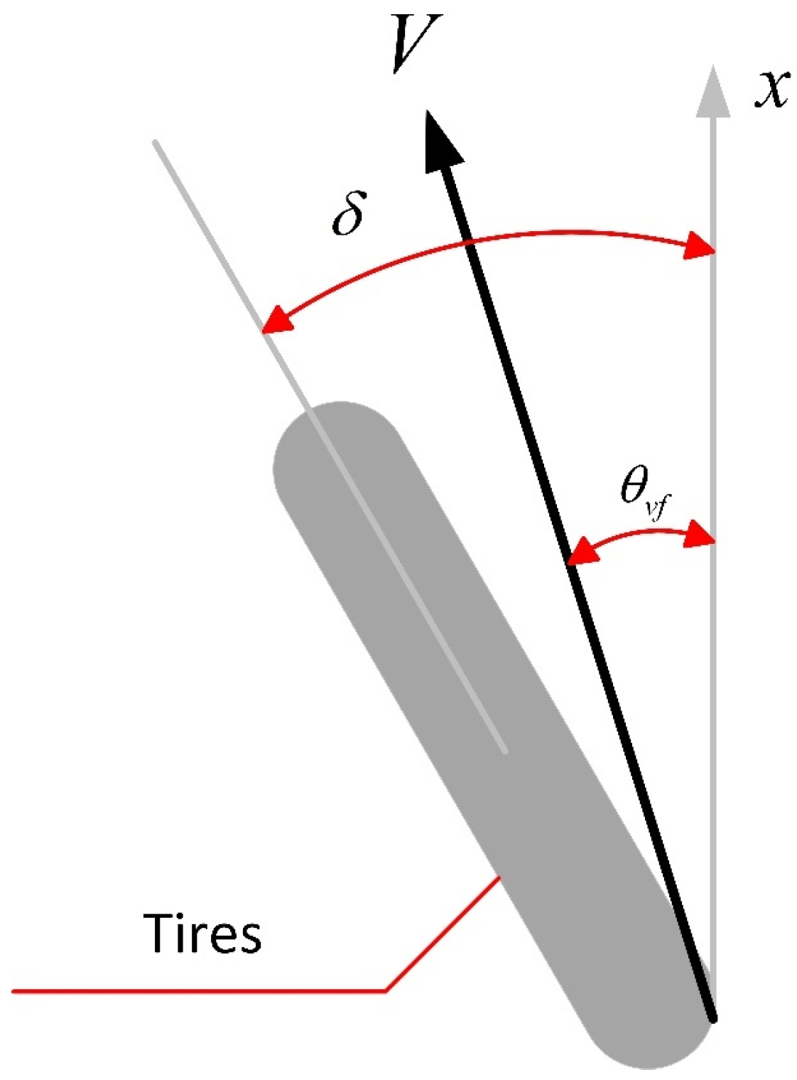
The magnitude of forces F y f and F y r acting on the vehicle tire in the y-axis direction is directly proportional to the tire’s lateral deflection angle, the side deflection angle shown in Figure 5.
According to the above Figure 5, the front wheel side cornering angle is
α f = δ θ v f .
The lateral force on the front axle of the vehicle can be expressed as
F y f = 2 C α f δ θ v f ,
where:
C α f —the lateral cornering stiffness of a single front wheel.
Similarly, the lateral force on the rear axle can be expressed as follows:
F y r = 2 C α r θ v r ,
where:
C α r —the lateral cornering stiffness of single rear wheel.

2.2.3. Transverse Two-Degree-of-Freedom Dynamics Model

As shown in Figure 6, the relationship between the vehicle’s front wheel side deflection angle and other state quantities can be visualized by the two-degree-of-freedom bicycle model:
Figure 6. Two-degree-of-freedom bicycle model.
Applsci 15 12245 g006
where:
C —the center of mass of the vehicle;
A , B —the centers of the front and rear axles, respectively;
l f , l r —the distances from A and B to the center of mass C , respectively;
v x , v y —the velocity on the x- and y-axes generated by the translation of the vehicle, respectively;
l f φ ˙ , l r φ ˙ —the linear velocities generated by the rotation of A and B around C , respectively.
Based on the positional relationship in Figure 6, we can obtain the following:
tan θ v f = v y + l f φ ˙ v x ,
tan θ v r = v y l r φ ˙ v x .
In general, the angle of the velocity vector is small; according to the small angle approximation principle tan δ δ , we can obtain the following:
θ v f = v y + l f φ ˙ v x ,
θ v r = v y l r φ ˙ v x .
Substituting Equations (14), (15), (18) and (19) into Equation (10) gives
m y ¨ + v x φ ˙ = 2 C α f δ y ˙ + l f φ ˙ v x + 2 C α r y ˙ l r φ ˙ v x .
Dividing both sides of the equal sign of Equation (20) simultaneously by m , to extract y ¨ , y ˙ , φ ˙ , and δ , respectively, which are collapsed into
y ¨ = 2 C α f + 2 C α r m v x y ˙ v x + 2 C α f l f 2 C α r l r m v x φ ˙ + 2 C α f m δ .
Similarly, substituting Equations (14), (15), (18) and (19) into Equation (12) yields
I z φ ¨ = 2 l f C α f δ y ˙ + l f φ ˙ v x 2 l r C α r y ˙ l r φ ˙ v x .
Both sides of the equal sign of Equation (22) are simultaneously divided by I z , to extract y ¨ , y ˙ , φ ˙ , and δ , respectively, which are collapsed into
φ ¨ = 2 l f C α f 2 l r C α r I z v x y ˙ 2 l f 2 C α f + 2 l r 2 C α r I z v x φ ˙ + 2 l f C α f I z δ .
As can be seen from Figure 6, the above dynamics studies are based on the vehicle coordinate system, but the actual study of dynamics problems is mostly based on the geodetic coordinate system, so there is also a need for coordinate conversion; the speed of the vehicle in the vehicle coordinate system and the geodetic coordinate system are converted into the following relationship:
X ˙ = v x cos φ v y sin φ Y ˙ = v x sin φ + v y cos φ .
Integrating Equations (21), (23) and (24), the state equations of the two-degree-of-freedom dynamics model of the vehicle are obtained as follows:
y ¨ = 2 C α f + 2 C α r m v x y ˙ v x + 2 C α f l f 2 C α r l r m v x φ ˙ + 2 C α f m δ φ ¨ = 2 l f C α f 2 l r C α r I z v x y ˙ 2 l f 2 C α f + 2 l r 2 C α r I z v x φ ˙ + 2 l f C α f I z δ X ˙ = v x cos φ v y sin φ Y ˙ = v x sin φ + v y cos φ .

2.3. Establishment of a Generalized Dynamics Model of “Steering Robot—Controlled Vehicle”

The output of the steering robot model is defined according to Equation (6) as x 1 , i.e., the angular position of the DC motor.
The input to the controlled vehicle model is defined according to Equation (25) as δ , i.e., the front wheel angle of rotation.
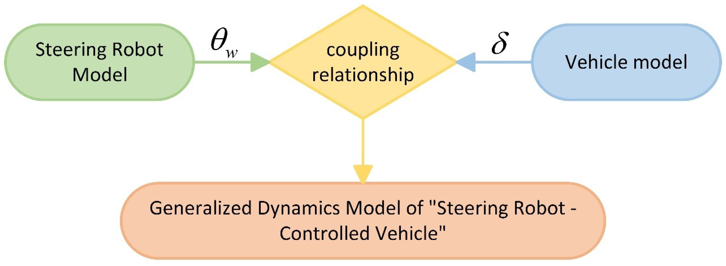
According to Figure 7, two of the three elements (steering robot model and controlled vehicle model) of the generalized dynamics model of the “steering robot-controlled vehicle” have been completed, and it is only necessary to find the coupling relationship between the angular position of the DC motors and the angle of the front wheels to be constructed.
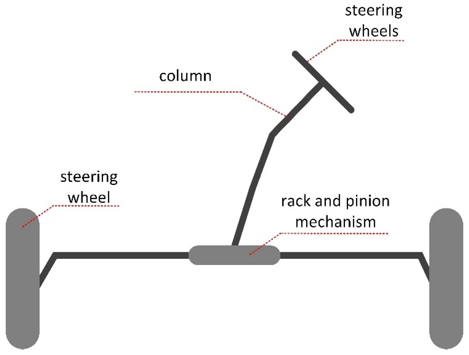
According to Figure 3, the angular position of the DC motor is equal to the angular position of the steering wheel, and the problem is transformed into finding the transformational relationship between the angular position of the steering wheel and the angle of rotation of the front wheel.
As shown in Figure 8, in the case of a rack and pinion steering structure, for example, the input from the steering wheel is fed through the steering rod to the gears, and then output from the rack to the steering wheel. That is, the angular position of the steering wheel multiplied by the gear ratio of the rack and pinion mechanism is equal to the front wheel turning angle.
There are many types of driveline structures, rack and pinion, recirculating ball, but what they all have in common is that they all have a fixed transmission ratio.
Define the transmission ratio of the drive train as k s , the steering wheel angle is expressed as θ s , and the front wheel angle is δ , so as to obtain the conversion relationship between the steering wheel angle and the front wheel angle:
δ = θ s k s .
Equations (6), (25) and (26) are combined to obtain the state equations of the generalized dynamics model of “steering robot-controlled vehicle”:
y ¨ = 2 C α f + 2 C α r m v x y ˙ v x + 2 C α f l f 2 C α r l r m v x φ ˙ + 2 C α f m π 180 k s θ w φ ¨ = 2 l f C α f 2 l r C α r I z v x y ˙ 2 l f 2 C α f + 2 l r 2 C α r I z v x φ ˙ + 2 l f C α f I z π 180 k s θ w X ˙ = v x cos φ v y sin φ Y ˙ = v x sin φ + v y cos φ θ ¨ w = k m k e J R + B J θ ˙ w + k m J R u + h t ,
where:
θ w —the angular position of the steering robot’s DC motor in angular units;
h t —the load item, h t = T L J ;
u —the voltage across the armature;
R —the armature circuit resistance;
k e —inverse electromotive force constant;
k m —the electromagnetic torque constant;
B —the motor damping factor;
J —the moment of inertia of the motor output shaft;
C α f —the lateral cornering stiffness of a single front wheel;
C α r —the lateral cornering stiffness of single rear wheel;
l f , l r —the distances from the center of gravity to the front and rear axles, respectively;
φ —yaw angle position.
The proposed generalized dynamics model couples the planar 2-DOF lateral–yaw model with the DC-motor model of the steering robot via the equivalent steering linkage. In conventional vehicle models, the front-wheel angle is treated as an external input, and the remaining states are computed, conditional on the front-wheel angle. However, in a driving-robot setup, the control command is the motor voltage. Consequently, a conventional model is naturally suited only for designing a cascaded MPC+PID architecture. In contrast, the generalized dynamics takes the control voltage directly as its input and propagates it to the vehicle states through the motor and steering linkage, making it suitable for designing an integrated MPC for the steering robot.

2.4. Integrated MPC Controller Design

2.4.1. Linear State Space Equations

Equation (27) is used as the model basis to design the integrated MPC controller, which is transformed into state space equation form:
χ ˙ = A χ + B μ + D ,
where:
χ = y ˙ φ ˙ X Y θ w θ ˙ w T ;
A = 2 C α f + 2 C α r m v x v x + 2 C α f l f 2 C α r l r m v x 0 0 2 C α f m π 180 k s 0 2 l f C α f 2 l r C α r I z v x 2 l f 2 C α f + 2 l r 2 C α r I z v x 0 0 2 l f C α f I z π 180 k s 0 sin φ 0 0 0 0 0 cos φ 0 0 0 0 0 0 0 0 0 0 1 0 0 0 0 0 k m k e J R + B J ;
B = 0 0 0 0 0 k m J R T ;
D = 0 0 v x cos φ v x sin φ 0 h t T ;
control volume: μ = u .

2.4.2. Linear Model Discretization

Discretization of Equation (28) using the forward Euler method is as follows:
χ ˙ = χ k + 1 χ k T = A χ k + B μ k + D k ,
Tidied up, it is as follows:
χ k + 1 = T A + 1 χ k + T B μ k + T D k .
Let A k = T A + 1 , B k = T B , D K k = T D K k ; obtain the discrete state space equation:
χ k + 1 = A k χ k + B k μ k + D k k η k = C k χ k ,
where:
C k = 0 1 0 0 0 0 0 0 0 1 0 0 ;
The output is φ ˙ Y T .

2.4.3. Predictive Modeling

The iteration of discrete equations is as follows:
χ k + 1 = A k χ k + B k μ k + D k k χ k + 2 = A k 2 χ k + A k B k μ k + A k D k k + B k μ k + 1 + D k k + 1 χ k + 3 = A k 3 χ k + A k 2 B k μ k + A k 2 D k k + A k B k μ k + 1 + A k D k k + 1 + B k μ k + 2 + D k k + 2 χ k + N p = A k N p χ k + A k N p 1 B k μ k + + A k N p N c 1 B k μ k + N c + A k N p 1 D k k + + D k k + N p 1 .
The output equation iteration is as follows:
η k + 1 = C k A k χ k + C k B k μ k + C k D k k η k + 2 = C k A k 2 χ k + C k A ˜ k B ˜ k μ k + C k A k D k k + C k B k μ k + 1 + C k D k k + 1 η k + 3 = C k A k 3 χ k + C k A k 2 B k μ k + C k A k 2 D k k + C k A k B k μ k + 1 + C k A k D k k + 1 + C k B k μ k + 2 + C k D k k + 2 η k + N p = C k A k N p χ k + C k A k N p 1 B k μ k + + C k A k N p N c 1 B k μ k + N c + C k A k N p 1 D k k + + C k D k k + N p 1 .
The prediction equation is obtained by collapsing Equation (33):
ϒ k = Ψ χ k + Θ U k + Γ Φ k ,
where:
ϒ k = η k + 1 η k + 2 η k + N c η k + N p ;   Ψ = C k A k C k A k 2 C k A k N c C k A k N p ;   Γ = C k 0 0 C k A k C k 0 C k A k N p 1 C k A k N p 2 C k ;
Θ = C k B k 0 0 C k A k B k C k B k 0 C k A k N c 1 B k C k A k N c 2 B k C k B k C k A k N c B k C k A k N c 1 B k C k A k B k C k A k N p 1 B k C k A k N p 2 B k C k A k N p N c 1 B k ;   Φ k = D k k D k k + 1 D k k + N p 1 ;
U k = μ k μ k + 2 μ k + N c T

2.4.4. Cost Function Design

The reference path is given by the upper-level path planner: ϒ r e f = φ ˙ r e f Y r e f T .
Design the following cost function:
J = ϒ ϒ r e f T Q ϒ ϒ r e f + U T R U + ρ ε 2 ,
where:
Q —the output weighting matrix;
R —the control weighting matrix;
ρ —the relaxation factor weights;
ε —the relaxation factor.
Expanding from Equation (35), we obtain the following:
J = Ψ χ + Θ U + Γ Φ ϒ r e f T Q Ψ χ + Θ U + Γ Φ ϒ r e f + U T R U + ρ ε 2 .
Let E = Ψ χ + Γ Φ ϒ r e f . Substituting Equation (36), we obtain the following:
J = E + Θ U T Q E + Θ U + U T R U + ρ ε 2 = E T Q E + E T Q Θ U + Θ U T Q E + U T Θ T Q Θ U + U T R U + ρ ε 2 ,
where:
E T Q Θ U , Θ U T Q E —transposed to each other and are one-element matrices, i.e., E T Q Θ U = Θ U T Q E .
We can obtain the following:
J = E T Q E + 2 E T Q Θ U + U T Θ T Q Θ U + U T R U + ρ ε 2 = U T Θ T Q Θ + R U + 2 E T Q Θ U + E T Q E + ρ ε 2 .
The cost function is transformed into a structure with respect to the control quantity U , where E T Q E is independent of U , so it is discarded.
Obtain the final cost function:
J = U T Θ T Q Θ + R U + 2 E T Q Θ U + ρ ε 2 .
Written as a secondary planning standard type, it is
J = 1 2 U ˜ T H U ˜ + f T U ˜ ,
where:
U ˜ = U ε ;   H = 2 Θ T Q Θ + R 0 0 2 ρ ;   f = 2 E T Q Θ 0 .

2.4.5. Design of Constraints

In the field of vehicle path tracking, the ultimate control quantity is the front wheel angle, regardless of whether a vehicle two-degree-of-freedom model or a three-degree-of-freedom model or an error model is used. The constraints of the MPC controllers designed based on these models are for the front wheel angle, while the control quantity of the integrated MPC controller for path tracking of the steering robot designed in this paper is the voltage of the steering robot’s motor; therefore, this paper needs to convert the constraints for the front wheel angle into the constraints for the steering robot’s motor voltage.
Assuming that there are constraints against the front wheel angle of rotation,
δ min < δ < δ max .
According to Equation (26), we can know that θ s = δ k s . Now, the above constraints for the front wheel angle can be transformed into constraints for the steering wheel angle:
θ s min < θ s < θ s max .
According to Figure 3, we can see that the steering robot is fixed on the steering wheel and the relative position of the steering robot to the steering wheel does not change. In other words, the steering wheel angle θ s and the steering robot motor angle θ w are always equal. Therefore, the constraints for the steering wheel angle can be transformed into constraints for the steering robot motor angle:
θ w min < θ w < θ w max .
In discrete systems, θ w k + 2 = θ w k + 1 + T θ ˙ w k + 1 ; moment k + 2 is also required to satisfy the constraints of Equation (43):
θ w min < θ w k + 2 < θ w max .
It can be rewritten as
θ w min θ w k + 1 T < θ ˙ w k + 1 < θ w max θ w k + 1 T .
where:
θ ˙ w —the state quantity in the generalized dynamics model developed in this paper.
According to Equation (31), we can obtain the following:
θ ˙ w k + 1 = A k θ ˙ w χ k + B k θ ˙ w μ k + D k θ ˙ w k .
Substituting Equation (46) into Equation (45) yields the following:
μ min < μ < μ max .
where:
μ min = θ w min θ w k + 1 T A k θ ˙ w χ k D k θ ˙ w k B k θ ˙ w ;   μ max = θ w max θ w k + 1 T A k θ ˙ w χ k D k θ ˙ w k B k θ ˙ w ;
θ w min = θ s min = δ min k s ;   θ w max = θ s max = δ max k s ;
θ w k + 1 = θ w k + T θ ˙ w k .
Equation (47) is the transformed constraint against the steering robot motor voltage. The parameters therein can all be obtained by calling the results of the current calculation in the integrated MPC controller.

2.5. The Integrated MPC Optimization Problem

Based on the preceding derivation, the Integrated MPC optimization problem can be described as follows:
min U ˜ 1 2 U ˜ T H U ˜ + f T U ˜ s . t .   δ min < δ k + i | k < δ max
The control variable sequence calculated for each cycle is as follows:
μ k μ k + 2 μ k + N c
Take the first control variable μ k as the control variable output for the current cycle.
Regarding the constraint on δ , during computation, it can be transformed in real time into a constraint on the control variable μ via Equation (47).

2.6. Simulation Tests

In this paper, the performance of the integrated MPC controller is verified by joint simulation with CarSim and Simulink.
To evaluate the comprehensive performance of the integrated MPC controller and the cascaded MPC+PID controller, two simulation scenarios were designed: (1) double-lane-change path tracking under high- and low-speed conditions, used to assess tracking accuracy and real-time performance; and (2) straight-line steady-state tracking with and without crosswind, used to assess controller robustness. Both controllers were tested under the same vehicle model, actuator limits, and constraints.

2.6.1. Double-Lane-Change Path Tracking

High-speed condition is as follows: vehicle speed 70 km/h, simulation duration 10 s, sampling period 10 ms.
Low-speed condition is as follows: vehicle speed 40 km/h, simulation duration 15 s, sampling period 10 ms.
We use the RMS (root-mean-square), Peak (maximum absolute error), and P95 (95th percentile) of the lateral error e y as the evaluation metrics for tracking accuracy; let N denote the total number of samples. The formulae for the metrics are as follows:
RMS = 1 N k = 1 N e y k 2
Peak = max 1 k N e y k
P 95 = q u a n t i l e e y 1 N , 0.95
The real-time performance metrics are worst-case execution time T max , average per-update solve time T A v g , and utilization ratio ρ A v g ; the formulae are as follows:
T max = max 1 k N t s o l v e k
T A v g = 1 N k = 1 N t s o l v e k
ρ A v g = T A v g T
Each MPC update solves a convex QP with interior-point-convex.

2.6.2. Robustness Evaluation Testing

The vehicle tracks a straight reference path at a target speed of 60 km/h. The disturbance is a crosswind modeled as an equivalent lateral force applied at the vehicle’s center of mass:
F y w i n d = 0.015 m g sin 0.4 π t
The robustness evaluation metric is the RMS, Peak, and P95 of the lateral error.
The parameters of the vehicles and driving robots used in the simulation tests are presented in Table 1 and Table 2.

3. Results and Discussion

3.1. High-Speed Condition

The core parameters of the integrated MPC controller for the high-speed condition are shown in Table 3.

3.1.1. Comparison of Tracking Performance Under High-Speed Condition

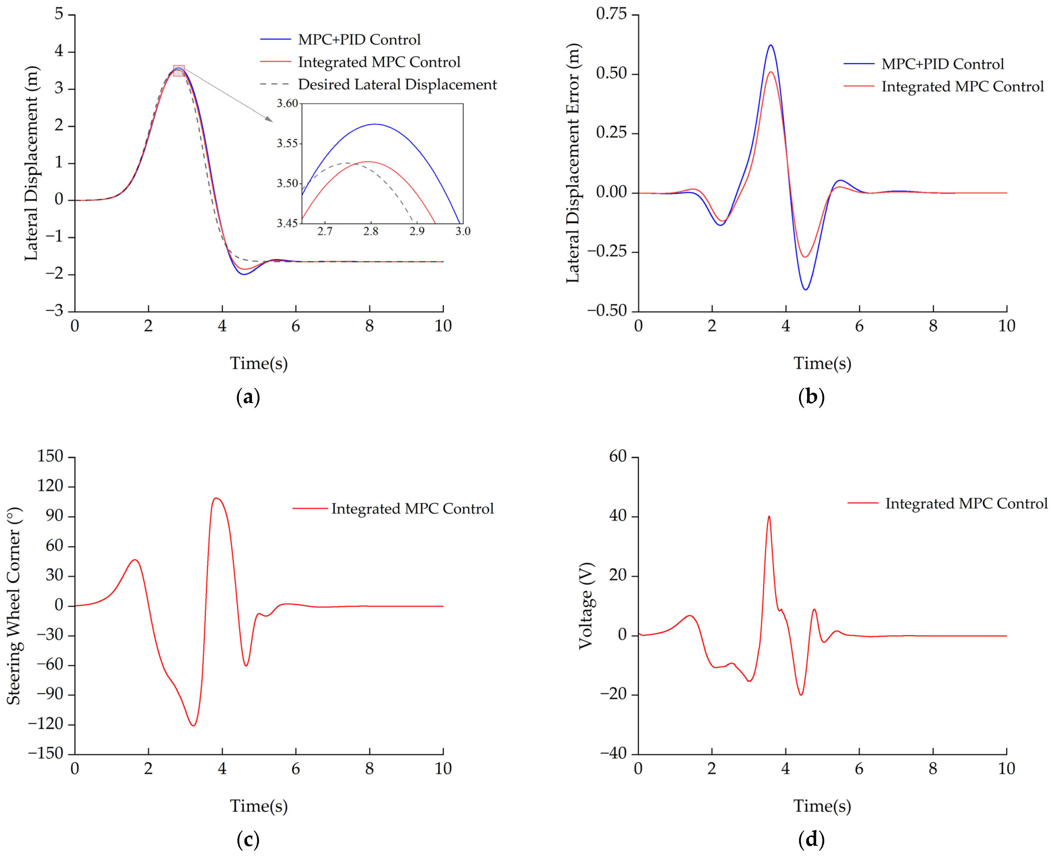
As shown in Figure 9a,b, we can see the following:
Both controllers complete the double-lane-change, but the Integrated MPC adheres more closely to the desired path around the peak and return phases. In the zoomed view, the Integrated MPC exhibits a smaller overshoot and less phase lag, while the cascaded MPC+PID departs more from the reference near the apex. This indicates a higher path-tracking accuracy for the Integrated MPC under fast, high-dynamic maneuvers.
The Integrated MPC yields a lower peak error, faster decay, and shorter ringing, returning to zero more quickly. The cascaded scheme shows a higher, sharper peak and a longer settling time. Mechanistically, the Integrated MPC jointly optimizes path tracking and actuator dynamics within one problem, anticipating actuator limits and dynamics and thereby avoiding the inter-layer error accumulation and extra phase lag inherent to cascaded designs.
Figure 9c,d illustrate that the Integrated MPC drives the actuator with smooth, non-saturating commands that remain within physical limits and without high-frequency chatter—evidence of feasibility and constraint satisfaction in the high-speed condition.
The tracking accuracy is evaluated using the RMS, Peak, and P95 of the lateral error.
According to Table 4, the Integrated MPC outperforms the cascaded MPC+PID across all three metrics in the high-speed condition:
The RMS drops from 0.17368 m to 0.13492 m (−22.3%), indicating a lower overall error level throughout the maneuver.
The Peak drops from 0.62321 m to 0.51082 m (−18.0%), reflecting a smaller worst-case lateral deviation during the most demanding phases of the DLC.
The P95 drops from 0.44708 m to 0.36798 m (−17.7%), showing a thinner upper tail of the error distribution, i.e., fewer large deviations for most of the time.
In the high-speed condition, the Integrated MPC provides meaningful, across-the-board reductions in lateral-tracking error, translating into a higher transient robustness and a larger safety margin, while maintaining a comparable settling time to the cascaded MPC+PID baseline.

3.1.2. Real-Time Performance Under High-Speed Condition

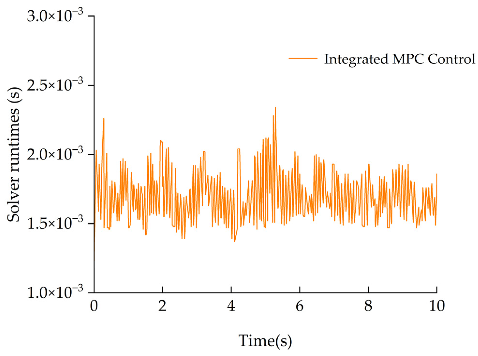
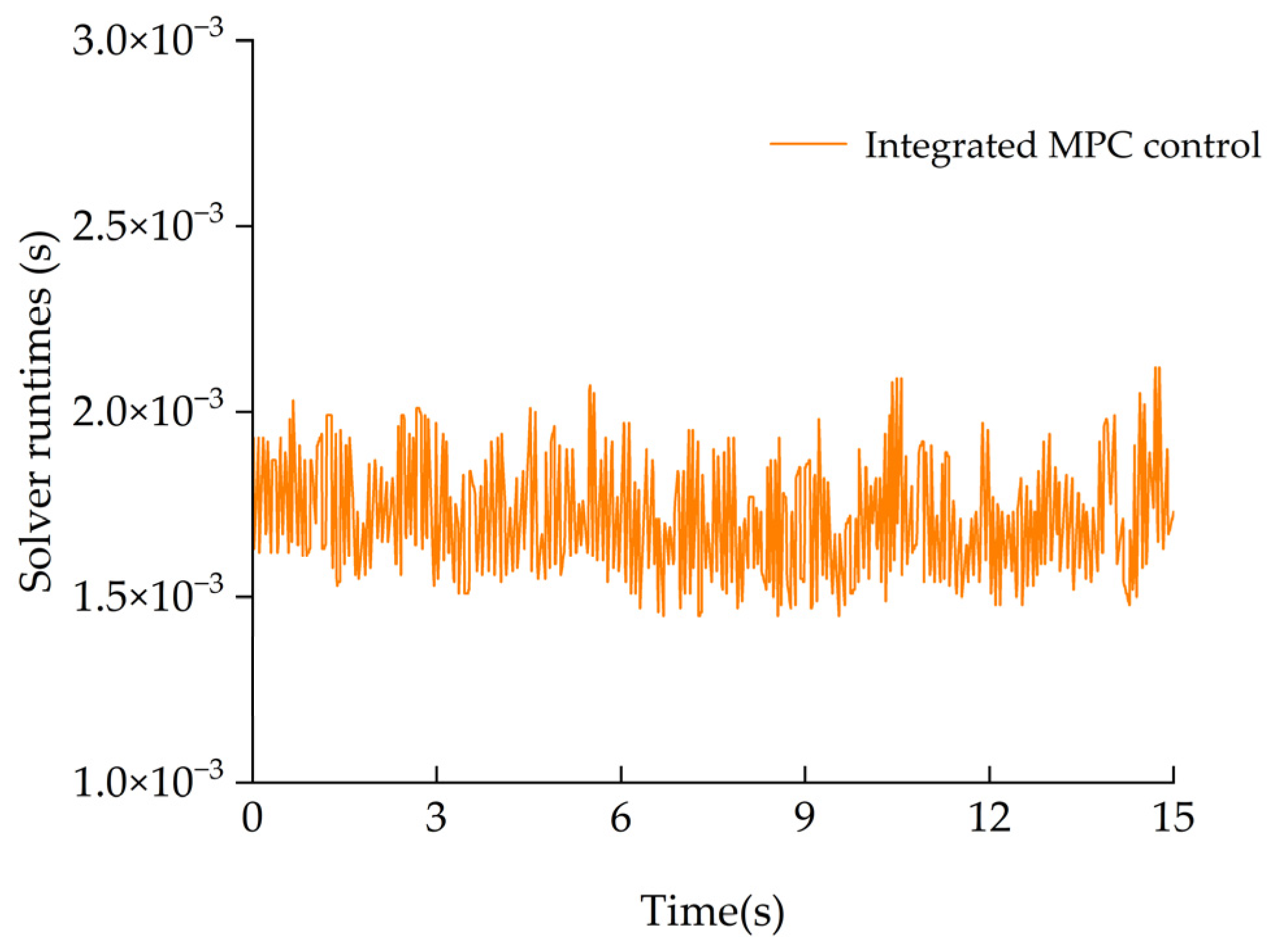
Figure 10 shows the per-step solver runtime of the integrated MPC at high speed. The runtime remains bounded with no upward drift, clustering around 1.5 ms with only occasional small spikes that quickly decay back to the steady band and stay well below the vertical axis limit.
According to Table 5, In the high-speed condition, we use fixed-step control with Sampling period T at 10 ms. The per-update solver time is logged and summarized as follows: the worst-case execution time T max is 2.340 ms; the average per-update solve time T A v g is 1.697 ms; and the utilization ratio ρ A v g is 0.17.
The controller satisfies hard real-time requirements at T = 10 ms.

3.2. Low-Speed Condition

The core parameters of the integrated MPC controller for the low-speed condition are shown in Table 6.

3.2.1. Comparison of Tracking Performance Under Low-Speed Condition

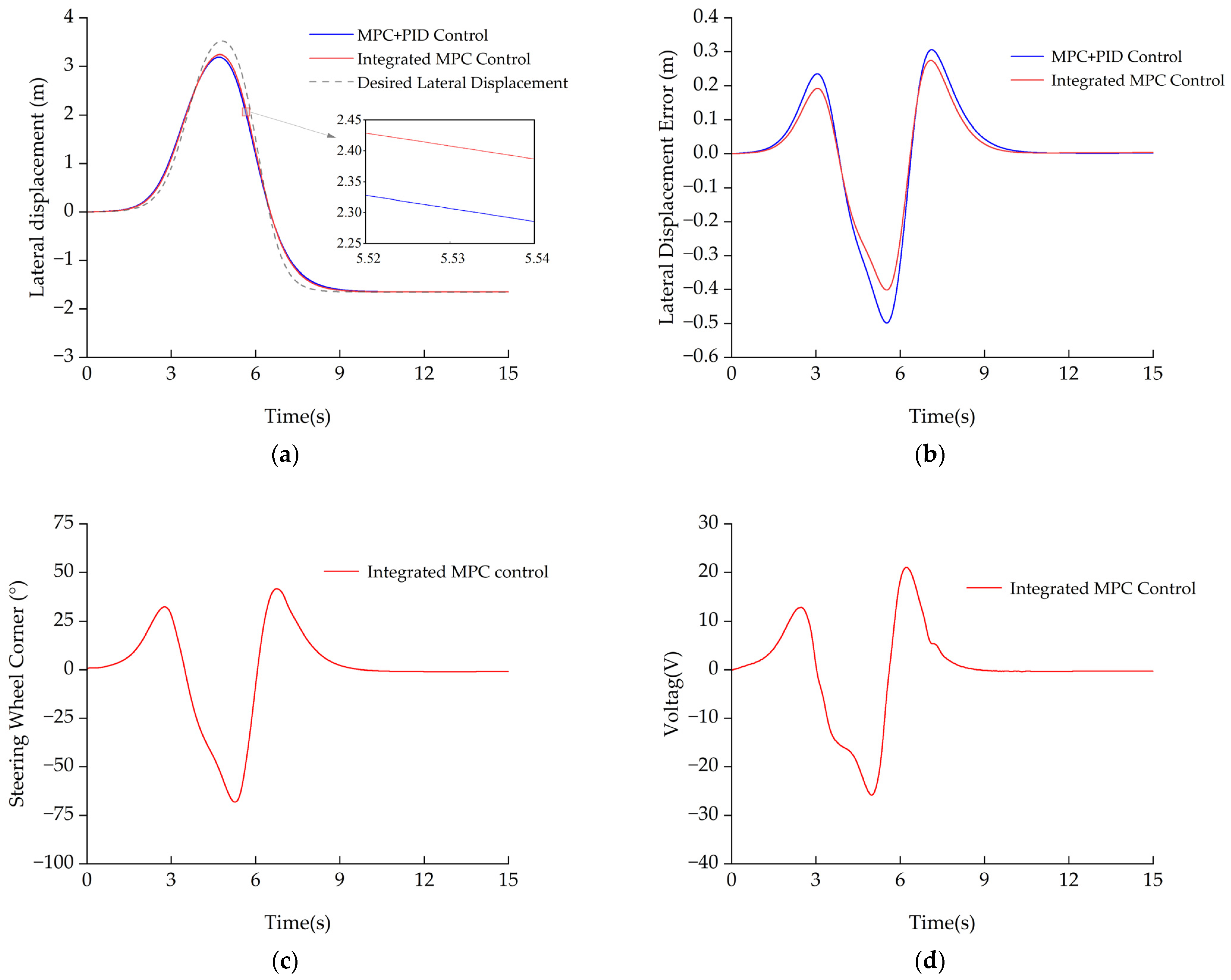
As shown in Figure 11, we can see the following:
Both controllers complete the DLC maneuver. Compared with the cascaded MPC+PID, the Integrated MPC follows the desired path more closely around the apex and during the return phase, with a smaller overshoot and a smoother transition back to the steady state.
Although the overall errors are small at low speed, the Integrated MPC exhibits a lower peak error, faster decay, and weaker oscillations around zero, indicating better damping and convergence.
The angle profile is smooth, with reversals consistent with the two-lane changes, and the peak remains well within mechanical limits. The control voltage is concentrated during the two lane-change phases and quickly returns near zero; the amplitudes and duration imply a comfortable safety margin for the actuator.
In the low-speed condition, both approaches are feasible, but the Integrated MPC consistently provides tighter apex tracking, quicker error attenuation, and smoother control effort, demonstrating speed-robust advantages rather than benefits limited to high-speed cases.
The tracking accuracy is evaluated using the RMS, Peak, and P95 of the lateral error.
As shown in Table 7, the Integrated MPC outperforms the cascaded MPC+PID on all three metrics in the low-speed condition:
The RMS decreases by 17.0%, indicating a lower overall error level over the whole maneuver.
The Peak drops by 19.5%, reflecting smaller worst-case excursions at the most demanding instants.
The P95 is reduced by 18.9%, showing a compressed upper tail for 95% of the timeline.

3.2.2. Real-Time Performance Under Low-Speed Condition

The concurrent reductions in RMS, Peak, and P95 provide coherent evidence that, even in low-speed DLC, the integrated formulation improves both the typical and extreme tracking behavior by avoiding the cascade-induced error build-up and serial phase lag.
Figure 12 illustrates the per-step solver runtime of the Integrated MPC in the low-speed condition. The runtime remains tightly bounded over the entire horizon, showing small fluctuations around roughly 1.5–2.0 ms with only occasional, limited spikes and no upward drift.
In the high-speed condition, we use fixed-step control with Sampling period T at 10 ms. The per-update solver time is logged and summarized as follows: the worst-case execution time T max is 2.12 ms; the average per-update solve time T A v g is 1.717 ms; and the utilization ratio ρ A v g is 0.172.
The controller satisfies hard real-time requirements at T = 10 ms.

3.3. Robustness Evaluation

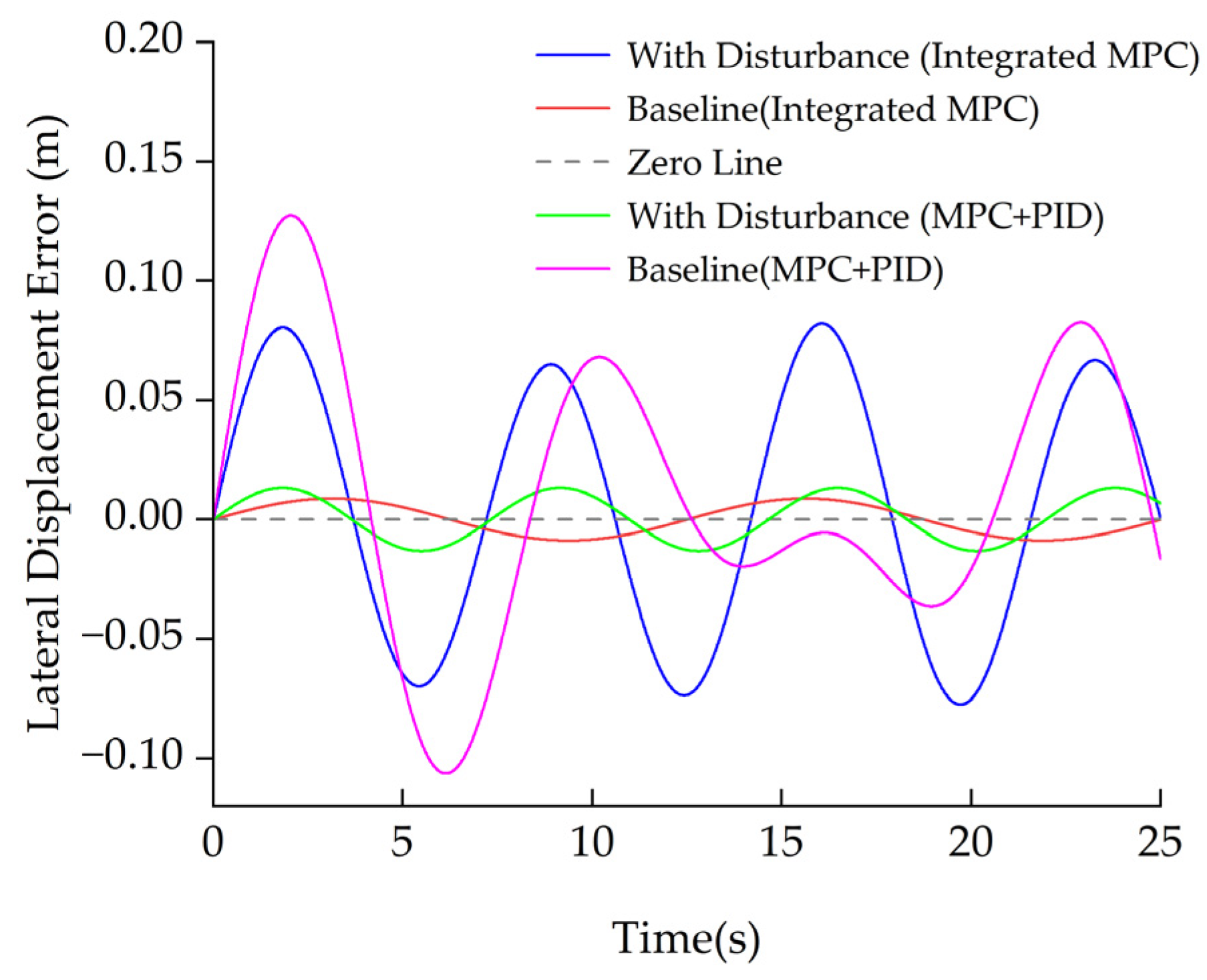
Figure 13 shows the time histories of the lateral error for the Integrated MPC and Cascaded MPC+PID under baseline and sinusoidal crosswind conditions (the zero-error line is indicated by a dashed line). Visual inspection reveals the following:
  • Integrated MPC: The baseline (red) stays tightly around the zero line with small, symmetric micro-oscillations. Under crosswind (blue), the error follows a near-periodic pattern synchronized with the disturbance but remains bounded with no noticeable drift; within each cycle, the error returns rapidly to the zero neighborhood, and the envelope stays stable over time, never approaching the vertical plotting limits.
  • Cascaded MPC+PID: Both baseline (magenta) and disturbed (green) cases exhibit larger low-frequency oscillations and more evident phase lag. Under the same disturbance, the return to zero is slower and the error envelope is wider, indicating weaker disturbance rejection—consistent with the error accumulation and serial delay inherent to cascaded structures where the actuator PID loop limits the overall robustness.
  • Takeaway: For the same external disturbance, the Integrated MPC keeps the trajectories closer to the zero line with a tighter envelope, evidencing a stronger disturbance rejection and larger safety margins, whereas the cascaded MPC+PID shows broader excursions and a slower recovery, reflecting inferior overall robustness.
The evaluation metrics are the RMS, Peak, and P95 of the lateral error.
The results indicate that both controllers satisfy the ±0.15 m constraint in straight-line tracking, while the Integrated MPC provides a larger robustness margin. Without disturbance (Baseline), its RMS/Peak/P95 are 34%/33%/33% lower than those of the cascaded MPC–PID. With a sinusoidal crosswind, the Integrated MPC improves over the cascaded MPC–PID by 9.7%/35.6%/30.8%, respectively.
MPC inherently provides strong robustness by predicting the system evolution, enforcing constraints, and correcting disturbance-induced deviations through receding-horizon optimization. PID, lacking explicit prediction and constraint handling, exhibits weaker disturbance rejection and is sensitive to tuning. In the cascaded MPC+PID architecture, the overall robustness is limited by the actuator PID loop—the weakest link—and further degraded by the error accumulation and serial phase lag across layers. In contrast, the Integrated MPC solves path tracking and actuator control within a single optimization, thus yielding stronger disturbance rejection and larger safety margin.

3.4. Summary

This chapter presents a Simulink–CarSim co-simulation study of the tracking accuracy, real-time performance, and robustness of the integrated MPC, benchmarked against the conventional cascaded MPC+PID. As shown in Table 4 and Table 7 (high/low-speed performance), Table 5 and Table 8 (real-time metrics), and Table 9 (robustness under model mismatch and crosswind), the Integrated MPC outperforms the cascaded baseline across all metrics. Mechanistically, MPC predicts the system evolution, enforces constraints, and corrects disturbance-induced deviations via a receding horizon, whereas PID lacks explicit prediction/constraint handling and is sensitive to tuning. In the cascaded MPC+PID architecture, the overall performance is limited by the actuator-side PID (the weakest link) and further degraded by inter-layer error accumulation and serial phase lag. In contrast, by solving path tracking and actuator control within a single optimization, the Integrated MPC avoids cascade effects, delivering higher tracking accuracy, stronger disturbance rejection, and a larger safety margin.

4. Conclusions

This paper presented an Integrated MPC formulation for steering-robot path tracking that optimizes the robot voltage directly and embeds physical steering-angle limits as linear-inequality voltage constraints inside the optimizer. Compared with a cascaded MPC+PID baseline, the integrated design avoids inter-layer error accumulation and extra phase lag while guaranteeing actuator-level feasibility.
Under a Simulink–CarSim co-simulation, two scenarios were evaluated: double-lane-change (DLC) at 70/40 km/h and straight-line tracking with/without sinusoidal crosswind. The results consistently favor the proposed controller.
  • High-speed DLC (70 km·h−1): The Integrated MPC reduces lateral-error RMS/Peak/P95 by 22.3%/18.0%/17.7% relative to the cascaded baseline, adheres more closely to the reference around the maneuver apex, and yields smoother, non-saturating actuator commands;
  • Low-speed DLC (40 km·h−1): Reductions of 17.0%/19.5%/18.9% in RMS/Peak/P95 demonstrate that benefits persist beyond high-dynamic conditions;
  • Real-time feasibility: With T = 10 ms, the per-update solve time clusters around 1.7 ms on average, with worst-case execution time ≈ 2.1~2.3 ms, giving utilization ratio ≈ 0.17—comfortably within hard real-time;
  • Robustness (straight + crosswind): Both controllers satisfy the ±0.15 m constraint. Without disturbance, the integrated MPC is lower in RMS/Peak/P95 than the cascaded design by roughly 34%/33%/33%. With sinusoidal crosswind, the Integrated MPC further improves over the cascaded scheme by 9.7%/35.6%/30.8% on RMS/Peak/P95, indicating stronger disturbance rejection and larger safety margins.
Overall, the Integrated MPC delivers tighter tracking, reduced extremes, and provable constraint satisfaction while meeting strict timing, making it a compelling choice for deployment on proving-ground steering robots to perform high-precision path-tracking tasks for vehicle testing and calibration.

Author Contributions

Conceptualization, Y.H. and L.T.; methodology, L.Y. and Y.H.; software, Y.L.; validation, L.T. and Y.C.; formal analysis, Y.H. and C.Y.; investigation, Y.H. and C.Y.; resources, L.T.; data curation, L.Y. and Y.C.; writing—original draft preparation, L.Y.; writing—review and editing, Y.H. and L.Y.; visualization, Y.L.; supervision, L.T.; project administration, Y.C.; funding acquisition, Y.H. All authors have read and agreed to the published version of the manuscript.

Funding

This work has been supported by the National Key Research and Development Program of China (2022YFB2503302), the National Natural Science Foundation of China (52225212, 52272418, U22A20100, and 5217120774), the Project of Faculty of Agricultural Equipment of Jiangsu University (NZXB20210103), and the Liaoning Province’s unveiling and leading project (Science and Technology Breakthroughs Special Project) (2023JH1/10400099).

Institutional Review Board Statement

Not applicable.

Informed Consent Statement

Not applicable.

Data Availability Statement

The data presented in this study are available on request from the corresponding author.

Conflicts of Interest

Author Liwei Tian was employed by the company Shenyang Shenda Connected Vehicle Collaborative Innovation Center Co., Ltd. The remaining authors declare that the research was conducted in the absence of any commercial or financial relationships that could be construed as a potential conflict of interest.

References

  1. Chen, G.; Yuan, J. Nonlinear dynamics analysis of shift manipulator for robot driver considering multiple revolute clearance joints and variable load. Mech. Based Des. Struct. Mach. 2020, 49, 596–614. [Google Scholar] [CrossRef]
  2. Chen, G.; Chen, S.; Langari, R.; Li, X.; Zhang, W. Driver-behavior-based adaptive steering robust nonlinear control of unmanned driving robotic vehicle with modeling uncertainties and disturbance observer. IEEE Trans. Veh. Technol. 2019, 68, 8183–8190. [Google Scholar] [CrossRef]
  3. Chen, G.; Su, S. Driver-behavior-based robust steering control of unmanned driving robotic vehicle with modeling uncertainties and external disturbance. Proc. Inst. Mech. Eng. Part D J. Automob. Eng. 2020, 234, 1585–1596. [Google Scholar] [CrossRef]
  4. Su, S.; Chen, G. Lateral robust iterative learning control for unmanned driving robot vehicle. Proc. Inst. Mech. Eng. Part I J. Syst. Control Eng. 2020, 234, 792–808. [Google Scholar] [CrossRef]
  5. Wang, H.; Chen, G.; Zhang, W. A method for vehicle speed tracking by controlling driving robot. Trans. Inst. Meas. Control 2019, 42, 1521–1536. [Google Scholar] [CrossRef]
  6. Chen, G.; Lu, W.; Mei, J.; Wang, L.; Zhang, W. Longitudinal robust dynamic programming control for driving robot vehicles with performance self-learning. Int. J. Control 2024, 98, 2304–2314. [Google Scholar] [CrossRef]
  7. Wang, Z.; Zhou, X.; Ren, S.; Chen, W.; Wang, H.; Wang, J. Preview path tracking control for autonomous vehicle with actuator saturation. In Proceedings of the 36th Chinese Control and Decision Conference (CCDC), Xi’an, China, 25–27 May 2024; pp. 2729–2734. [Google Scholar] [CrossRef]
  8. Zheng, R.; Li, R. Autonomous Vehicle Collision Avoidance Path Planning and F-MPC Tracking Control. Int. J. Fuzzy Syst. 2025. [Google Scholar] [CrossRef]
  9. Lin, D.; Qiu, J.; Tang, M.; Zhang, Q.; Xu, S.; Song, H. Obstacle avoidance path planning and trajectory tracking of unmanned logistics vehicle based on MPC. In Proceedings of the 2024 China Automation Congress (CAC), Qingdao, China, 1–3 November 2024; pp. 1190–1195. [Google Scholar] [CrossRef]
  10. Zhao, J.; Li, Y.; Yang, L. Path tracking control for autonomous vehicles based on MPC combined with adaptive potential field optimization. In Proceedings of the 2024 IEEE 19th Conference on Industrial Electronics and Applications (ICIEA), Kristiansand, Norway, 5–8 August 2024; pp. 1–6. [Google Scholar] [CrossRef]
  11. Švancar, J.; Haniš, T. MPC-based path-tracking algorithm using a priori known road friction condition for the over-actuated subscale vehicle platform. In Proceedings of the 2024 18th International Conference on Control, Automation, Robotics and Vision (ICARCV), Dubai, United Arab Emirates, 12–15 December 2024; pp. 1017–1022. [Google Scholar] [CrossRef]
  12. Ma, N.; Zhuang, H.; Kang, S.; Ge, P.; He, T.; Cui, Z. Autonomous driving intelligent vehicle overtaking path tracking based on MPC. In Proceedings of the 2024 IEEE 4th International Conference on Electronic Technology, Communication and Information (ICETCI), Changchun, China, 24–26 May 2024; pp. 520–524. [Google Scholar] [CrossRef]
  13. Bai, G.; Liu, S.; Zhou, B.; Huang, J.; Zheng, Y.; Elham, E. Path Tracking for Electric Mining Articulated Vehicles Based on Nonlinear Compensated Multiple Reference Points Linear MPC. World Electr. Veh. J. 2024, 15, 427. [Google Scholar] [CrossRef]
  14. Feng, K.; Li, X.; Li, W. Adaptive MPC path-tracking controller based on reinforcement learning and preview-based PID controller. Proc. Inst. Mech. Eng. Part D J. Automob. Eng. 2024; in press. [Google Scholar] [CrossRef]
  15. Wang, H.; Wang, C.; Zhao, L.; Hu, Y. Variable-parameter MPC Multi-objective Control for Intelligent Vehicle Path Tracking Based on Reinforcement Learning. China J. Highw. Transp. 2024, 37, 157–169. (In Chinese) [Google Scholar] [CrossRef]
  16. Ren, H.; Li, Y.; Wang, L.; Yang, L. Lateral path tracking control based on tube MPC. In Proceedings of the 2024 3rd International Symposium on Intelligent Unmanned Systems and Artificial Intelligence (SIUSAI ’24), New York, NY, USA, 17–19 May 2024; pp. 130–135. [Google Scholar] [CrossRef]
  17. Zhang, H.; Li, Y.; Wu, G. Tube-MPC Based Path Tracking for I Vehicle Considering Data-Driven Stable Region and External Disturbances; SAE Technical Paper 2025-01-8262; SAE International: Warrendale, PA, USA, 2025. [Google Scholar] [CrossRef]
  18. Yangin, V.B.; Yalcin, Y.; Akalin, O. A tunable explicit nonlinear MPC for a vehicle considering improved path tracking performance and computational efficiency. J. Mech. Sci. Technol. 2025, 39, 2877–2888. [Google Scholar] [CrossRef]
  19. Tuer, S.; Panahandeh, P.; Alghooneh, A.R.; Sun, C.; Zhang, R.; Ning, M. Real-time MPC for WATonoBus path tracking. In Proceedings of the 2024 IEEE 27th International Conference on Intelligent Transportation Systems (ITSC), Edmonton, AB, Canada, 24–27 September 2024; pp. 3233–3238. [Google Scholar] [CrossRef]
  20. Hou, Y.; Ren, Y.; Meng, S. Research on vehicle path tracking control based on MPC. In Proceedings of the 2022 6th International Conference on Electronic Information Technology and Computer Engineering (EITCE ’22), New York, NY, USA, 21–23 October 2022; pp. 449–453. [Google Scholar] [CrossRef]
  21. Bo, Y.; Guo, H.; Shen, C.; Liu, J. MPC-based path tracking controller design for intelligent driving vehicle. In Proceedings of the 2019 Chinese Control Conference (CCC), Guangzhou, China, 27–30 July 2019; pp. 3006–3011. [Google Scholar] [CrossRef]
  22. Tang, C.; Li, T.; Li, T.; Ma, J.; Xiong, H. All-wheel steering path tracking control for multi-axle vehicle based on adaptive MPC. In Proceedings of the 2024 4th International Conference on Computer, Control and Robotics (ICCCR), Shanghai, China, 19–21 April 2024; pp. 183–190. [Google Scholar] [CrossRef]
  23. Chen, M.; Ren, Y. MPC-based path tracking control for autonomous vehicle with multi-constraints. In Proceedings of the 2017 International Conference on Advanced Mechatronic Systems (ICAMechS), Xiamen, China, 6–9 December 2017; pp. 477–482. [Google Scholar] [CrossRef]
  24. Ma, N.; Kang, S.; Zhuang, H.; Ge, P.; He, T.; Cui, Z. A MPC-based mix function controller on path planning and path tracking of autonomous vehicles. In Proceedings of the 2024 IEEE 4th International Conference on Electronic Technology, Communication and Information (ICETCI), Changchun, China, 24–26 May 2024; pp. 525–530. [Google Scholar] [CrossRef]
  25. Zhou, Z.; Bao, Y. Path tracking control of autonomous vehicle based on MPC. In Proceedings of the 2024 3rd International Conference on Energy and Power Engineering, Control Engineering (EPECE), Chengdu, China, 23–25 February 2024; pp. 211–216. [Google Scholar] [CrossRef]
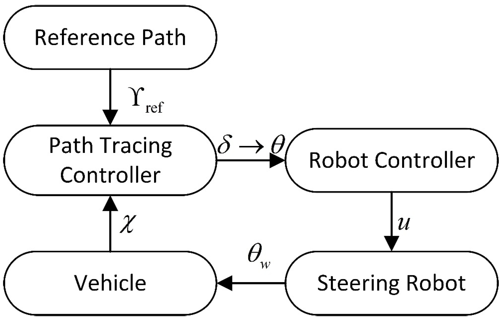
Figure 1. Conventional control structure.
Applsci 15 12245 g001
Figure 2. Integrated control structure.
Applsci 15 12245 g002
Figure 3. Schematic diagram of the mounting structure of the steering robot.
Applsci 15 12245 g003
Figure 4. Schematic diagram of vehicle coordinates.
Applsci 15 12245 g004
Figure 5. Schematic diagram of side cornering angle.
Applsci 15 12245 g005
Figure 7. Flow of generalized dynamics model construction.
Applsci 15 12245 g007
Figure 8. Mechanical structure of vehicle steering system.
Applsci 15 12245 g008
Figure 9. Simulation results of high-speed condition: (a) Lateral Displacement Comparison; (b) Lateral Displacement Error Comparison; (c) Change in Steering Wheel Corner; and (d) Change in Control Voltage.
Applsci 15 12245 g009
Figure 10. Real-time performance in high-speed condition.
Applsci 15 12245 g010
Figure 11. Simulation results of low-speed condition: (a) Lateral Displacement Comparison; (b) Lateral Displacement Error Comparison; (c) Change in Steering Wheel Corner; and (d) Change in Control Voltage.
Applsci 15 12245 g011
Figure 12. Real-time performance in the low-speed condition.
Applsci 15 12245 g012
Figure 13. Robustness evaluation (straight line + crosswind).
Applsci 15 12245 g013
Table 1. Parameters of the simulated vehicle.
ParametersValueParametersValue
m 1230 kg I z 1343 kg m 2
l 2.58 m C α f −56,864 N / rad
l f 1.22 m C α r −66,864 N / rad
k s 27
1 All parameters are explained in the paper.
Table 2. Parameters of the steering robot motor.
ParametersValueParametersValue
U n 48 V k m 0.72 Nm / A
I n 3.6 A k e 0.2 Vs / rad
n n 2000 r / min J 0.01 kg / m 2
R 1 Ω B 0.03 Ns / m
1 U n is rated voltage, I n is rated current, and n n is the rated speed.
Table 3. The core parameters of the integrated MPC controller for high-speed condition.
ParametersValueParametersValue
N p 10 N c 10
Q λ 1 × 10 3 0 0 3.4 R 1 . 5 × 10 5
δ min −30 ° δ max 30 °
1 Q λ is the diagonal block of the Q matric. 2 N p is the prediction horizon and N c is the control horizon.
Table 4. Path Tracking Accuracy Evaluation Metrics (high-speed condition).
GroupRMSPeakP95
Cascaded MPC+PID0.17368 m 0.62321 m 0.44708 m
Integrated MPC0.13492 m 0.51082 m 0.36798 m
Table 5. Integrated MPC real-time statistics in high-speed condition.
StatisticValueStatisticValue
T 10 ms T max 2.34 ms
T A v g 1.697 ms ρ A v g 0.17
Table 6. The core parameters of the integrated MPC controller for low-speed condition.
ParametersValueParametersValue
N p 10 N c 10
Q λ 1.3 × 10 3 0 0 3.6 R 1 . 5 × 10 5
δ min −30 ° δ max 30 °
1 Q λ is the diagonal block of the Q metric.
Table 7. Path Tracking Accuracy Evaluation Metrics (low-speed condition).
GroupRMSPeakP95
Cascaded MPC+PID0.17300 m 0.49843 m 0.41930 m
Integrated MPC0.143615 m 0.40146 m 0.34018 m
Table 8. Integrated MPC real-time statistics in the low-speed condition.
StatisticValueStatisticValue
T 10 ms T max 2.12 ms
T A v g 1.717 ms ρ A v g 0.172
Table 9. Robustness metrics (straight line + crosswind).
GroupRMSPeakP95
Baseline
(Integrated MPC)
0.00622 m 0.00880 m 0.00877 m
With Disturbance
(Integrated MPC)
0.05234 m 0.08209 m 0.07832 m
Baseline
(MPC+PID)
0.00942 m 0.01320 m 0.01316 m
With Disturbance
(MPC+PID)
0.05794 m 0.127440 m 0.11318 m
Disclaimer/Publisher’s Note: The statements, opinions and data contained in all publications are solely those of the individual author(s) and contributor(s) and not of MDPI and/or the editor(s). MDPI and/or the editor(s) disclaim responsibility for any injury to people or property resulting from any ideas, methods, instructions or products referred to in the content.