UGV Formation Path Planning Based on DRL-DWA in Off-Road Environments ^†

Abstract

Uneven terrains and complex obstacles in off-road environments present significant challenges to the stability and safety of vehicle path planning. This paper presents a hierarchical DRL-DWA path planning framework for unmanned ground vehicles (UGVs). At the global level, an energy-aware D* Lite algorithm generates cost-efficient waypoints considering both distance and energy consumption. At the local level, a deep reinforcement learning-enhanced DWA controller adaptively adjusts the weighting factors of evaluation functions in real time to ensure dynamic feasibility on rough terrain. The parameter selection is formulated as a Markov decision process (MDP), where a novel reward function based on elevation maps, vehicle pose, goal, and obstacle information guides the optimization for off-road navigation. Furthermore, the single UGV framework is extended to a multi-UGV system, where formation control is achieved through the leader–follower strategy. To evaluate the performance of our algorithm, we conduct experiments in 3D simulation environments featuring various terrains and obstacles. The results indicate that the proposed approach outperforms existing path planning techniques, showing a higher success rate and a lower average elevation gradient in uneven terrains.

1. Introduction

1.1. Research Motivation

Unmanned ground vehicles (UGVs) have gained widespread recognition for their capability to replace humans in performing tasks in hazardous environments [1]. They have been widely applied in various fields including wilderness search and rescue, forest firefighting, planetary exploration, and military operations. In contrast to on-road environments, off-road scenes often present uneven terrains and a wide array of static and dynamic obstacles, creating substantial difficulties for vehicle navigation.

Path planning aims to calculate a feasible route that can safely navigate to the target position without collision after the starting and target points are defined based on a certain environmental model [2]. Depending on the degree of knowledge about the environment, path planning is categorized into global path planning and local path planning. Global path planning is applicable to static scenarios, and its precision largely depends on the accuracy of environmental data acquisition. On the other hand, local path planning leverages real-time perception data from the sensor system, offering greater adaptability to dynamic environments. To enable UGVs to move efficiently and safely to the task area, path planning needs to be performed in advance [3].

A single UGV is usually limited by its operational efficiency and capabilities; therefore, a multi-UGV formation is more suitable for completing complex tasks. The multi-UGV system needs to have the ability to maintain formation, rapidly form and reconfigure formations, avoid internal collisions, and achieve flexible formation changes.

1.2. Literature Review

Path planning for off-road environments is usually divided into two stages: map construction and path searching. Cost maps are often considered binary, distinguishing between traversable and non-traversable areas, or represented as a continuous traversability score [4]. Various path planning methods can then be applied, such as search-based [5,6], sampling-based [7,8], and optimization-based [9,10] approaches.

The dynamic window approach (DWA) is another notable method [11] that directly searches for optimal control velocities. It achieves this by calculating the weighted sum of multiple evaluation functions in the velocity space. These velocities are constrained within a region known as the “dynamic window,” allowing the incorporation of UGV dynamics into the approach. However, these weighting factors are manually set based on expert experience. During the path planning process, as the relationship between the UGV and the environment changes, the requirements for each evaluation function become time-varying. The use of fixed weighting factors can thus lead to more collisions or situations where the UGV becomes trapped.

The rapid development of artificial intelligence has garnered significant attention from scholars, leading to the emergence of numerous learning-based local path planning schemes [12,13,14,15]. These learning-based methods demonstrate the ability to process high-dimensional input information, showing autonomy and flexibility in the field of vehicle autonomous navigation. However, most of them concentrate on flat indoor surfaces, making it challenging to apply them to cluttered rough terrain. To address this limitation, several studies have focused on learning to classify cost functions or cost maps from environmental features. For instance, Ref. [16] proposed a novel method that leverages unlabeled data to train a deep neural network, allowing the robot to effectively perceive and differentiate between various types of terrain surfaces, including grass, rocks, and paths. Ref. [4] investigated a statistical method to calculate cost maps directly from point cloud data and a learning-based method that employs point cloud data as input to an LSTM neural network for predicting the IMU response, both of which enabled local and global path planning for autonomous systems. Moreover, LiDAR-based traversability analysis has been investigated to improve terrain understanding in off-road driving. A recent study combining deep learning and Gaussian Process modeling achieved up to 14% higher precision than traditional methods, highlighting the importance of robust perception for safe UGV navigation [17].

Recently, there has been growing research interest in end-to-end methods for path planning in uneven environments [18]. Ref. [19] proposed a novel Navigation Multi-Modal Fusion Network and chose end-to-end supervised learning for training. Ref. [20] proposed a self-supervised near-to-far approach to help autonomous vehicles sense and understand the terrain ahead by utilizing unlabeled sensory data. Deep reinforcement learning (DRL) is another prominent category that enables learning directly from raw sensory data. In [21], multi-dimensional sensory data, including elevation maps, depth images, and robot orientations, were utilized as input to a DRL network to learn the navigation actions of the robot. Ref. [22] compared the effectiveness of four input types and introduced an attention mechanism to highlight the relative importance of the inputs. Ref. [23] decoupled perception and navigation into two different DRL models, introduced an attention mask to pinpoint regions with reduced stability, and finally evaluated the proposed method on real-world uneven terrains. Building upon this, a multi-objective DRL framework (AC-MOPP) was proposed to improve robustness under complex terrain and varying weather by integrating heuristic rules and prioritized experience replay [24]. Moreover, a Bird’s-Eye View (BEV)-based perception–planning framework was introduced to enhance vehicle adaptability and autonomous decision-making in extreme off-road scenarios [25]. These studies highlight the trend toward perception-aware and multi-objective reinforcement learning for robust off-road navigation.

Nevertheless, it is important to note that the velocities produced directly by the DRL network may violate the vehicle’s non-holonomic constraints, making them dynamically infeasible [26]. Moreover, as the distance between the start and the destination increases, training the DRL agent becomes more challenging due to longer episodes and sparse rewards. This scenario often leads to the issue of getting stuck in local optima during the learning process [13].

1.3. Contributions

In this study, global planning based on a pre-built environment representation is performed. This approach aims to avoid relying solely on local planning, which can easily lead the UGV to suboptimal solutions, such as a dead end [11,27]. Subsequently, the local path planner following the global route finds a dynamically feasible trajectory for the UGV, ensuring collision avoidance with obstacles detected by the onboard sensors. Unlike previous works that only apply reinforcement learning to tune the DWA parameters, our approach introduces a hierarchical integration that combines a global energy-aware D* Lite planner with a DRL-enhanced DWA local controller. Moreover, this framework is further extended to leader–follower formation navigation in off-road environments, representing a comprehensive scheme that jointly addresses global–local coupling, dynamic feasibility, and multi-agent coordination.

Building upon our preliminary work presented in [28], which introduced a hierarchical path planning framework using deep reinforcement learning in off-road settings, this paper further extends the approach by integrating a DRL-enhanced DWA controller and applying it to multi-UGV formation navigation. The key innovations of our work are as follows:

• A hierarchical large-scale off-road path planning scheme is presented in this paper, which consists of two components: (1) a global path planner based on D* Lite for calculating a roughly feasible global path, and (2) a local motion controller for calculating a dynamically feasible path and conducting obstacle avoidance.
• DRL and DWA are combined to complement each other’s strengths and overcome their respective limitations. The weighting factors of the DWA evaluation functions are adaptively adjusted by the DRL network, and the final optimal control velocities are calculated by DWA, which ensures that they are dynamically feasible.
• We expand the single UGV into a multi-UGV system and compare the proposed algorithm to prior navigation methods using real-world terrain data. Experimental results demonstrate that the proposed method considerably enhances the success rate of path planning while avoiding various obstacles and non-traversable terrain when the sacrifice of trajectory length and travel time is almost negligible.

1.4. Organization

This paper is organized in the following manner. In Section 2, we formulate the parameter selection process for DWA as a Markov decision process (MDP) and discuss why reinforcement learning is a suitable approach. Section 3 provides a comprehensive description of our hierarchical path planning algorithm. Section 4 examines the simulation results of our algorithm, and finally, Section 5 summarizes the key findings and contributions of this work.

2. Problem Formulation

This work focuses on a UGV incorporating a 3D LiDAR system capable of sensing within a $radius$ range. The local elevation map ${\mathbf{E}}_t$ in a robot-centric coordinate frame at time instant t is obtained from sensor measurements. x, y, z represent the position of the UGV. Key positional elements include the vehicle’s location $P_{ugv}=(x,y)$, obstacle positions $P_{obst}=(x_{obst},y_{obst})$, and the target goal $P_{goal}=(x_{goal},y_{goal})$. The UGV’s orientation is determined through three rotational parameters: pitch (${\theta }_{pitch}$), roll (${\theta }_{roll}$), and yaw (${\theta }_{yaw}$). Smaller pitch and roll angles make the driving process of the UGV more stable, and these are obtained from the elevation map and the coordinates and yaw of the vehicle in this study.

Figure 1 illustrates the architecture of our path planning algorithm. The gray part above is the global path planner, which generates a finite set of waypoints with the least cost to guide the local path planning process. The blue part below is the local path planner. The DRL neural network dynamically generates the weight parameters for DWA based on the global information, vehicle pose, and sensor information. Subsequently, DWA generates dynamically feasible velocities for the UGV considering its dynamic constraints.

In the adaptive tuning of DWA parameters, the parameter selection depends solely on the present state of the UGV, without considering the previous state. As a result, this property allows the problem to be formally represented as a Markov decision process (MDP) characterized by five fundamental components: $\langle S,A,P,R,\gamma \rangle$. The state space S includes information that describes the current driving state of the UGV, such as the local elevation map, vehicle pose, obstacle information, and goal information. The action space A represents the set of adjustable DWA parameters that need adaptive learning. P is the state transition probability matrix. R is the reward function, and $\gamma \in [0,1]$ is the discount factor for future rewards.

At each time step t, the agent chooses an action $a_t$ according to its environmental observation $s_t$ and the policy $\pi \left(a_t\right|s_t)$. It then receives a reward $r_{t+1}$ and a new observation $s_{t+1}$, which is determined by the state transition probability $p\left(s_{t+1}\right|s_t,a_t)$.

The discounted return $G_t$ can be used to evaluate a sequence of actions in the long run:

$$G_t=r_{t+1}+\gamma r_{t+2}+{\gamma }^2{r}_{t+3}+{\gamma }^3{r}_{t+4}+\dots$$

(1)

Calculating the expected discounted reward produces the action-value function, which is commonly utilized for evaluating the value of a given state–action pair:

$$q_{\pi }(s,a)=\mathbb{E}\left[G_t\right|S_t=s,A_t=a].$$

(2)

Furthermore, as one of the criteria to evaluate the pros and cons of a policy $\pi$, the state-value function can be defined as the expectation of the action-value function:

$$V_{\pi }\left(s\right)={\mathbb{E}}_a\left[q_{\pi }(s,a)\right]=\sum _{a\in A}\pi \left(a\right|s)·q_{\pi }(s,a).$$

(3)

We utilize the neural network $\pi \left(a\right|s,\theta )$ to approximate the policy $\pi \left(a\right|s)$, and we employ the neural network $V(s,\omega )$ to approximate $V_{\pi }\left(s\right)$, which guides policy updates during training. Therefore, the problem of adaptive tuning of the DWA parameters can be expressed as finding an optimal policy that maximizes the average reward:

$${\theta }^{*}=\underset{\theta }{argmax}{\overline{r}}_{\pi }.$$

(4)

Since $\pi$ is parameterized by $\theta$, the average reward is a function of $\theta$. Gradient-based optimization algorithms can be employed to search for optimal policy. Finally, the DWA parameter at the current time instant can be obtained from the fully trained policy $\pi$.

3. Proposed Solution

3.1. Global Path Planning

An enhanced D* Lite algorithm, which considers both the distance and energy factors affecting the mobility of UGVs, is employed for global path planning. The main advantage of D* Lite is its ability to dynamically update the path in a changing environment without recalculating the entire path from scratch, so the search efficiency is higher. When UGVs receive new environmental information from external communication equipment or map updates, such as cave-in or fire ahead, D* Lite has the capability for rapid re-planning.

(1) Environment model: The Digital Elevation Model (DEM) is a discrete mathematical representation of the earth’s surface landform, typically represented by an elevation matrix composed of regular grid elements, defined as

$$z=dem(x,y).$$

(5)

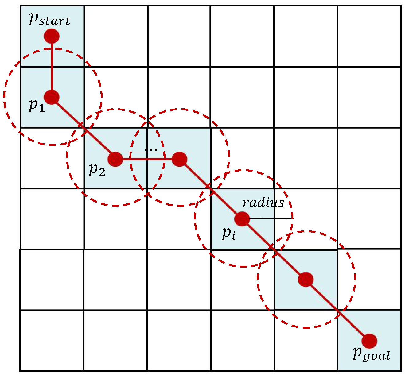
To facilitate path planning, the grids in these raster data are abstracted into nodes. The research areas are then converted into weighted graph representations utilizing eight-connected connectivity, and the edges in the graph represent the motion costs between adjacent nodes, as illustrated in Figure 2.

(2) Energy-cost model: According to the energy expenditure framework [29], it is assumed that the UGVs travel at a fixed velocity v throughout the whole journey. Then the energy consumed from node n to node m is easily calculated as $Mg{d}_{m,n}(\mu cos{\varphi }_{m,n}+sin{\varphi }_{m,n})$, where M represents the UGV’s mass, g denotes gravitational acceleration, and $\mu$ stands for the coefficient of friction. The term $d_{m,n}$ corresponds to the 3D Euclidean distance between nodes m and n, while ${\varphi }_{m,n}$ indicates the angle of inclination.

Assuming that the maximum output force to counteract gravity and friction is $F_{max}=P_{max}/v$, where $P_{max}$ representing the UGV’s maximum power capacity, the maximum slope angle that the UGV can exceed is given by

$${\varphi }_f=arcsin\left({\displaystyle \frac{F_{max}}{Mg\sqrt{{\mu }^2+1}}}\right)-arctan\left(\mu \right).$$

(6)

To avoid the loss of traction on a steep surface, the slope angle must be less than ${\varphi }_s$, which is defined by (7), where ${\mu }_s$ denotes static friction.

$${\varphi }_s=arctan({\mu }_s-\mu ).$$

(7)

As analyzed above, the critical uphill slope limit can be defined as

$${\varphi }_{up}=min({\varphi }_f,{\varphi }_s).$$

(8)

When the UGVs travel downhill, the slope angle at which the resultant external force on the UGVs be zero is termed the critical braking angle [30], which can be calculated by,

$${\varphi }_{down}=-arctan\left(\mu \right).$$

(9)

When $\varphi <{\varphi }_{down}$, the UGV will accelerate because of its own gravity. To maintain a constant velocity, the UGV needs to brake, which consumes negligible energy. It is worth noting that if ${\varphi }_{m,n}>{\varphi }_{up}$, it means that the UGV cannot drive along the straight line linking node m and node n, but it may still take a detour from node m to node n. Here, following [30], the heuristic energy cost from node m to node n is defined as

$$\begin{array}{c}\hfill e_{m,n}=\left\{\begin{array}{cc}{\displaystyle \frac{Mg(z_n-z_m)}{sin{\varphi }_{up}}}(\mu cos{\varphi }_{up}+sin\left({\varphi }_{up}\right)),\hfill & \hfill \mathrm{if}{\varphi }_{m,n}>{\varphi }_{up}\\ Mg{d}_{m,n}(\mu cos{\varphi }_{m,n}+sin{\varphi }_{m,n}),\hfill & \hfill \mathrm{if}{\varphi }_{up}>{\varphi }_{m,n}>{\varphi }_{down}\\ 0,\hfill & \hfill \mathrm{otherwise}.\end{array}\right.\end{array}$$

(10)

(3) Global planning based on D* Lite: D* Lite uses reverse search from goal to start and selects the next exploration node according to the minimum $key$-value as defined in (11)–(13). It continuously propagates and updates the path information until convergence at the target location is achieved. When selecting the node to expand, it first compares the $k_1$-value and selects the node with the minimum $k_1$-value. When $k_1$-value is equal, it selects the node with the minimum $k_2$-value.

$$key\left(n\right)=[k_1\left(n\right);k_2\left(n\right)].$$

(11)

$$k_1\left(n\right)=min(g\left(n\right),rhs\left(n\right))+h(c,n)+k_m.$$

(12)

$$k_2\left(n\right)=min(g\left(n\right),rhs\left(n\right)).$$

(13)

The function $g\left(n\right)$ quantifies the currently known minimum path cost from the target location to node n; $rhs\left(n\right)$ is an estimate of the cost from the goal to the node n that is updated based on new information. $h(c,n)$ is a heuristic function that calculates an estimated traversal cost between the initial node c and node n. It is used to guide the algorithm to compute and update only g-values associated with the shortest path from origin to destination. These three values can be calculated from the global cost map. $k_m$ is a key modifier, indicating the distance that the UGV has moved.

Based on simple additive weighting, the cost of moving from node m to node n can be calculated by (14), where $\alpha$ is a weighting factor adjustable according to user preferences.

$$c(n,n^{\prime })=\alpha ·d_{m,n}+(1-\alpha )·e_{m,n}.$$

(14)

(4) Combination of global and local planning: Applying the above global cost map to the D* Lite algorithm, the minimum cost global path can be calculated. During the hierarchical planning process, each global path node $P_i$ serves as an intermediate target for local path optimization. When the distance between the UGV and the waypoint $P_i$ is less than the effective $radius$, as shown in Figure 3, the next waypoint $P_{i+1}$ becomes the new optimization target. This iterative target-switching mechanism continues until final destination attainment. The strategy of utilizing global path nodes as sequential waypoints enables the vehicle to maintain velocity consistency while effectively navigating around challenging terrain features, thereby preventing convergence to suboptimal local solutions.

3.2. Local Path Planning

The dynamic window approach (DWA) generates a search space and maximizes the objective function to directly select the optimal translational and rotational velocities from the feasible velocities within the dynamic window. This approach aims to generate a collision-free trajectory that conforms to the dynamic constraints of UGVs [11].

(1) Search space generation: The DWA restricts the trajectory to an arc by directly controlling the velocity pair $(v,\omega )$.

Equation (15) illustrates that the UGVs are limited by both maximum and minimum linear velocities and angular velocities.

$$V_s=\left\{(v,\omega )\right|v\in [v_{min},v_{max}]\wedge \omega \in [{\omega }_{min},{\omega }_{max}]\}.$$

(15)

The dynamic window is defined as (16), which indicates that the search space is limited to the actual admissible velocities constrained by acceleration in a single forward time step.

$$\begin{array}{cc}\hfill V_d=\left\{(v,\omega )\right|& v\in [v_c-{\dot{v}}_{max}·▵t,v_c+{\dot{v}}_{max}·▵t],\hfill \\ & \omega \in [{\omega }_c-{\dot{\omega }}_{max}·▵t,{\omega }_c+{\dot{\omega }}_{max}·▵t]\},\hfill \end{array}$$

(16)

where $v_c$, ${\omega }_c$ are the current velocities of the UGV, ${\dot{v}}_{max}$, ${\dot{\omega }}_{max}$ are the maximum linear and angular accelerations, and $▵t$ is the time step.

To ensure that the UGVs can come to a stop in front of obstacles while decelerating at their current speed under maximum acceleration, the search space is pruned as shown in (17), where function $dist(v,\omega )$ quantifies the distance to the closest obstacle.

$$\begin{array}{cc}\hfill V_a=\left\{(v,\omega )\right|& v\le \sqrt{2·dist(v,\omega )·{\dot{v}}_{max}},\hfill \\ & \omega \le \sqrt{2·dist(v,\omega )·{\dot{\omega }}_{max}}\}.\hfill \end{array}$$

(17)

The final velocity search space of UGVs is defined as

$$V_r=V_s\cap V_d\cap V_a.$$

(18)

(2) Objective function optimization: Once the predicted trajectories for each velocity in the search space have been calculated, the trajectory corresponding to the $(v,\omega )$ pair that maximizes the objective function defined in (19) is selected as the locally optimal path. $\alpha$, $\beta$, and $\gamma$ are weight factors that can be adjusted manually according to specific requirements. Additionally, $\sigma$ represents the normalization coefficient.

$$\begin{array}{c}\hfill G(v,\omega )=\sigma [\alpha ·heading(v,\omega )+\beta ·dist(v,\omega )+\gamma ·velocity(v,\omega \left)\right].\end{array}$$

(19)

The function $heading(v,\omega )$ computes the angle between the forward orientation of the UGV along its predicted path and the target direction. This subfunction ensures rapid convergence of the UGV toward the target during movement. The function $dist(v,\omega )$ calculates the distance between the UGV’s predicted trajectory endpoint and the nearest obstacle. This subfunction helps to keep the UGV away from obstacles, thus ensuring safe navigation. The function $velocity(v,\omega )$ represents the forward velocity of the UGV. It is designed to ensure that the target is reached as quickly as possible, prioritizing efficiency in movement.

3.3. DRL Design

Reinforcement learning develops state–action mappings through environmental interaction, optimizing cumulative rewards [31]. This section defines the state space, action space, and reward function for path planning in uneven terrains and introduces the architecture of the DRL network.

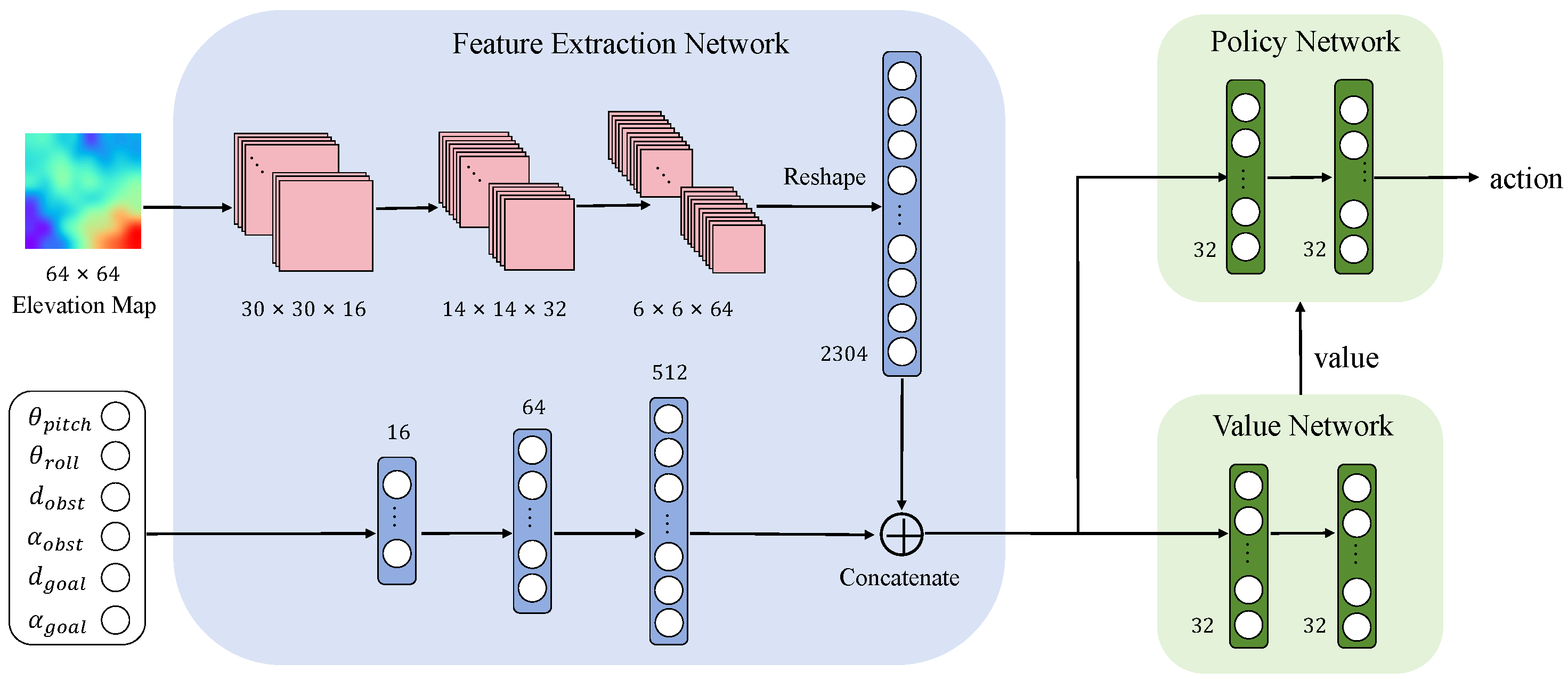
(1) State space: State describes the status of the agent with respect to the environment. The inputs to the DRL network include 2D local elevation maps ${\mathbf{E}}_t$, vehicle pose ${\theta }_{pitch}$, ${\theta }_{roll}$, obstacle information, and goal information. Obstacle information consists of nearest obstacle distance $d_{obst}=d(P_{ugv},P_{nearest})$ and the relative bearing angle between the current heading and nearest obstacle direction ${\alpha }_{obst}$. Goal information consists of the distance to the goal $d_{goal}=d(P_{ugv},P_{goal})$ and the goal bearing angle ${\alpha }_{goal}$ relative to the current heading.

$$S=[{\mathbf{E}}_t,{\theta }_{pitch},{\theta }_{roll},d_{obst},{\alpha }_{obst},d_{goal},{\alpha }_{goal}].$$

(20)

(2) Action space: In reinforcement learning, an action represents the agent’s decision in a given state. In the context of the DWA, the UGV chooses a speed that maximizes an objective function composed of three weighted subfunctions. In addition to the weight factors associated with the objective function, the time period T significantly influences the objective function’s final score. Consequently, the action space in the DRL-DWA network consists of four actions, as expressed in (21). Since each evaluation function has been normalized, its weight factor is defined as a continuous value ranging from $[0,1]$, indicating the level of importance given to the corresponding evaluation function. The time period T is defined as a continuous value within the range of [0,2], representing the duration for simulating the UGV’s motion at the sampled speed.

$$A=[\alpha ,\beta ,\gamma ,T].$$

(21)

(3) Reward: Reward provides environmental feedback for the agent’s state–action pairs, enabling behavior evaluation and policy improvement. This reinforcement mechanism prioritizes high-reward actions, progressively guiding the agent toward optimal target states.

Dangerous situations for the UGV can be categorized into three cases: (a) collision with obstacles; (b) beyond the map; and (c) pitch or roll angles exceeding 40°. Exploration is terminated either when the target is reached or when the UGV encounters any of these dangerous conditions. To prevent the agent from failing to improve its policy due to a lack of rewards during the lengthy navigation process, a dense reward function consisting of seven sub-reward functions is designed as (22), where the different $\lambda$ values are the weighing factors.

$$\begin{array}{cc}\hfill R_{tot}=& {\lambda }_1{R}_{succ}+{\lambda }_2{R}_{fail}+{\lambda }_3{R}_{wayp}+{\lambda }_4{R}_{goal}\hfill \\ & +{\lambda }_5{R}_{obst}+{\lambda }_6{R}_{grad}+{\lambda }_7{R}_{time}.\hfill \end{array}$$

(22)

The agent will receive a large positive reward $r_{succ}$ when the UGV successfully reaches the target. Conversely, if the UGV is in danger, the agent will receive a large negative reward $r_{fail}$. In addition, if the distance between the UGV and the temporary waypoint is less than the effective $radius$, the agent receives a positive reward denoted as $r_{wayp}$.

$$R_{succ}^t=\left\{\begin{array}{cc}{r}_{succ},\hfill & \mathrm{if}\mathrm{reach}\mathrm{target}\hfill \\ 0,\hfill & \mathrm{otherwise}.\hfill \end{array}\right.$$

(23)

$$R_{fail}^t=\left\{\begin{array}{cc}{r}_{fail},\hfill & \mathrm{if}\mathrm{in}\mathrm{danger}\hfill \\ 0,\hfill & \mathrm{otherwise}.\hfill \end{array}\right.$$

(24)

$$R_{wayp}^t=\left\{\begin{array}{cc}{r}_{wayp},\hfill & \mathrm{if}\mathrm{reach}\mathrm{waypoints}\hfill \\ 0,\hfill & \mathrm{otherwise}.\hfill \end{array}\right.$$

(25)

If the UGV is closer to the destination, the agent receives a positive reward of $r_{goal}$; otherwise, it receives a negative reward of $-r_{goal}$ as defined in (26). Similarly, if the UGV is closer to the obstacle, the agent receives a negative reward of $-r_{obst}$; otherwise, it receives a positive reward of $r_{obst}$ as defined in (27).

$$R_{goal}^t=\left\{\begin{array}{cc}{r}_{goal},\hfill & \mathrm{if}d(P_{ugv}^t,P_{goal})<d(P_{ugv}^{t-1},P_{goal})\hfill \\ -r_{goal},\hfill & \mathrm{if}d(P_{ugv}^t,P_{goal})>d(P_{ugv}^{t-1},P_{goal})\hfill \\ 0,\hfill & \mathrm{otherwise}.\hfill \end{array}\right.$$

(26)

$$R_{obst}^t=\left\{\begin{array}{cc}{r}_{obst},\hfill & \mathrm{if}dist(v^t,{\omega }^t)>dist(v^{t-1},{\omega }^{t-1})\hfill \\ -r_{obst},\hfill & \mathrm{if}dist(v^t,{\omega }^t)<dist(v^{t-1},{\omega }^{t-1})\hfill \\ 0,\hfill & \mathrm{otherwise}.\hfill \end{array}\right.$$

(27)

$R_{grad}$ is designed to encourage the agent to learn features that help avoid regions with high elevation gradients, as shown in (28). $r_{grad}$ is a small positive number.

$$R_{grad}^t=-▵{\mathbf{E}}^t\left(P_{ugv}^t\right)·r_{grad}.$$

(28)

The agent receives a small negative reward $r_{time}$ for each time step before reaching the final state.

$$R_{time}^t=r_{time}.$$

(29)

(4) Network architecture: Our DRL network of actor–critic architecture is based on Proximal Policy Optimization (PPO) because of its ease of use and good performance [32].

The network architecture is illustrated in Figure 4. As mentioned earlier, the DRL network utilizes elevation maps, vehicle pose, goal information, and obstacle information as inputs for determining the parameters of the DWA. The DRL network is divided into two main parts: a shared feature extraction network for the actor and critic, which extracts features from high-dimensional observations, and a fully connected network that maps these features to actions and values. In the image branch, we employ three stacked convolutional layers to extract features from the input elevation map and reshape the resulting feature maps into a latent vector representation. In the vector branch, we concatenate the remaining inputs and pass them through two fully connected layers. The outputs of these two branches are then merged as inputs for the policy network and value network, each containing two fully connected layers. The value network produces a state value that aids in improving future policies, while the policy network generates a 4D vector parameterizing the DWA controller.

The overall algorithm is shown in Algorithm 1.

Algorithm 1 Path planning based on DRL-DWA.

Initialization: Policy network with random parameters $\theta$, value network with random parameters $\omega$, discount factor $\gamma$ Training:     1: for episode = 1 to N do     2:       Initialize the start and end of navigation, the location and size of obstacles;     3:       for t = 1 to $timesteps$ do     4:             Observe the state $s_t$;     5:             Randomly sample $a_t$ according to $\pi (·|s_t,{\theta }_t)$;     6:             Perform DWA according to $a_t$;     7:             Observe new state $s_{t+1}$ and receive reward $r_{t+1}$;     8:             Update $\omega$ using temporal difference;     9:             Update $\theta$ using policy gradient;   10:             if reaching the target or being in danger then   11:                  break;   12:             end if   13:       end for   14: end for

3.4. Formation Control

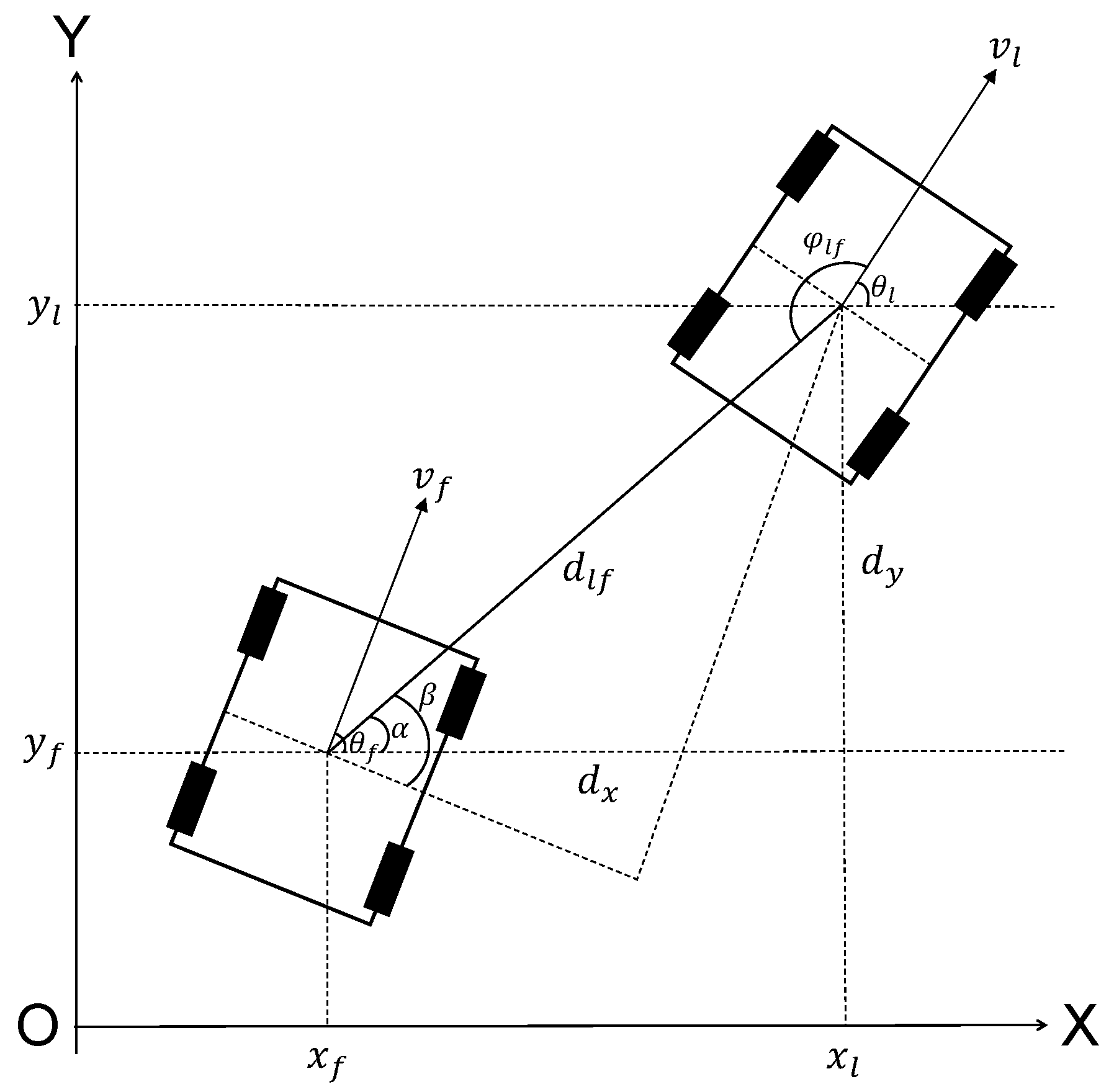
The leader–follower formation motion model between two vehicles is shown in Figure 5. The vehicle body length is $2h$, and the front axle length and rear axle length of the vehicle are both h. For a given UGV, h is a constant. The center-of-mass coordinates of the leader UGV are $(x_l,y_l,{\theta }_l)$, while those of the follower UGV are $(x_f,y_f,{\theta }_f)$. The leader UGV’s motion is characterized by linear velocity $v_l$ and angular velocity ${\omega }_l$, while the follower UGV operates with corresponding velocities $v_f$ and ${\omega }_f$. The relative positioning between UGVs is defined by three parameters: the inter-vehicle distance $d_{lf}$ between their centers of mass, the velocity alignment angle ${\phi }_{lf}$ between $v_l$ and $d_{lf}$, and the orientation angle $\alpha$ between $d_{lf}$ and the global X-axis. The straight-line distance between the center of mass of the leader UGV and the follower UGV is $d_{lf}$, which represents the relative distance between the leader and the follower. The angle between the linear velocity $v_l$ of the leader UGV and the straight-line distance $d_{lf}$ between the centers of mass is ${\phi }_{lf}$, which represents the relative angle between the leader and the follower. The angle $\alpha$ is the angle between the straight-line distance $d_{lf}$ between the centers of mass and the X-axis direction. The angle $\beta$ is the angle between the straight-line distance $d_{lf}$ between the centers of mass and the vertical direction of the follower’s linear velocity $v_f$.

According to Figure 5, the following angle relationships can be obtained:

$$\left\{\begin{array}{c}{\theta }_l=\pi -{\phi }_{lf}+\alpha \hfill \\ {\theta }_f={\displaystyle \frac{\pi }{2}}-\beta +\alpha .\hfill \end{array}\right.$$

(30)

Decompose the straight-line distance $d_{lf}$ between the centers of mass of the leading and the following UGV into $d_x$ along the X-axis and $d_y$ along the Y-axis, then

$$d_{lf}={d_x}^2+{d_y}^2,$$

(31)

$$\left\{\begin{array}{c}{d}_x=x_l-x_f=d_{lf}cos\alpha \hfill \\ d_y=y_l-y_f=d_{lf}sin\alpha .\hfill \end{array}\right.$$

(32)

Assume that the ideal distance and ideal angle between the leader and the follower are $d_{lf}^{id}$ and ${\phi }_{lf}^{id}$, respectively. Accordingly, $d_x^{id}$ and $d_y^{id}$ represent the components of the ideal distance along the X- and Y-axes. The error function can be expressed as

$$\left\{\begin{array}{c}{e}_x=d_x-d_x^{id}\hfill \\ e_y=d_y-d_y^{id}\hfill \\ e_{\theta }={\theta }_l-{\theta }_f.\hfill \end{array}\right.$$

(33)

The error function is differentiated and simplified to obtain the final error control model:

$$\left\{\begin{array}{cc}\dot{e_x}=\hfill & v_{l}sin{e}_{\theta }+h{\omega }_{l}cos{e}_{\theta }+(h+e_y){\omega }_f\hfill \\ & -d_{lf}^{id}{\omega }_{l}cos({\phi }_{lf}^{id}+e_{\theta })\hfill \\ \dot{e_y}=\hfill & v_{l}cos{e}_{\theta }-v_f+h{\omega }_{l}sin{e}_{\theta }-e_x{\omega }_f\hfill \\ & -d_{lf}^{id}{\omega }_{l}sin({\phi }_{lf}^{id}+e_{\theta })\hfill \\ \dot{e_{\theta }}=\hfill & {\omega }_l-{\omega }_f.\hfill \end{array}\right.$$

(34)

In order to make the error (Equation (34)) converge to zero, the linear velocity $v_f$ and angular velocity ${\omega }_f$ of the UGV are designed as the system control input:

$$\left\{\begin{array}{cc}{\omega }_f=\hfill & {\displaystyle \frac{-k_1\mathrm{sgn}\left(e_x\right){\left|e_x\right|}^{{\alpha }_1}-k_2\mathrm{sgn}\left(e_x\right){\left|e_x\right|}^{{\beta }_1}-v_{l}sin{e}_{\theta }}{h+e_y}}\hfill \\ \hfill & +{\displaystyle \frac{-h{\omega }_{l}cos{e}_{\theta }+d_{lf}^{id}{\omega }_{l}cos({\phi }_{lf}^{id}+e_{\theta })}{h+e_y}}\hfill \\ v_f=\hfill & k_3\mathrm{sgn}\left(e_y\right){\left|e_y\right|}^{{\alpha }_2}+k_4\mathrm{sgn}\left(e_y\right){\left|e_y\right|}^{{\beta }_2}+v_{l}cos{e}_{\theta }\hfill \\ & +h{\omega }_{l}sin{e}_{\theta }-e_x{\omega }_f-d_{lf}^{id}{\omega }_{l}sin({\phi }_{lf}^{id}+e_{\theta }).\hfill \end{array}\right.$$

(35)

Among them, the parameters $0<{\alpha }_1,{\alpha }_2<1$, ${\beta }_1,{\beta }_2>1$, $k_1,k_2,k_3,k_4>0$, $\mathrm{sgn}(·)$ is the symbolic function, and the calculation method is as follows:

$$\mathrm{sgn}\left(x\right)=\left\{\begin{array}{cc}1,\hfill & x>0\hfill \\ 0,\hfill & x=0\hfill \\ -1,\hfill & x<0.\hfill \end{array}\right.$$

(36)

The implementation steps of the unmanned vehicle formation control problem in an off-road environment are mainly divided into three steps: (1) The leader uses the DRL-DWA-based path planning method to plan the path according to the global cost map and sensor information. (2) The leader drives along the planned path, avoiding various obstacles in the environment. Simultaneously, the leader also needs to detect its own pose information in real time, use the distance–direction control strategy to generate the position information of the virtual UGV and send it to the follower. (3) The follower takes the position of the virtual UGV sent by the leader as the target, adjusts its own linear speed and angular velocity, and moves along the trajectory of the virtual UGV. The follower continuously detects the surrounding environmental information in real time. When encountering an obstacle, it waits in place for a while. When the leader passes, the follower will drive to the position of the leader’s UGV at the last moment. After avoiding the obstacle, the follower resumes the original trajectory and the formation is restored. To prevent mutual waiting in cluttered scenes, we add a lightweight priority-based tie-breaking rule as an extension of the leader–follower scheme: when a follower detects that the obstacle ahead is another UGV, right of way is granted according to a simple order (leader → follower closer to the goal → others); the lower-priority vehicle waits briefly and retries, while the higher-priority vehicle proceeds (with local replanning via DRL-DWA if needed).

Based on the DRL-DWA-based path planning algorithm proposed above, the leader–follower formation algorithm is shown in Algorithm 2.

Algorithm 2 A formation algorithm combining DRL-DWA-based path planning and leader–follower method.

Output: Global cost map, UGV position, obstacle information, target information Input: Formation trajectory     1: The leader uses the DRL-DWA-based path planning method to plan the path according to the global cost map and sensor information;     2: Use the leader–follower method to make the follower follow the leader at a certain distance and angle;     3: if Changes in the information surrounding the leader then     4:     Re-plan to avoid obstacles;     5: end if     6: if Follower encounters an obstacle then     7:     if obstacle is another UGV then     8:         Apply the priority rule (Leader → closer follower → others);     9:         if self has priority then   10:              Replan locally (DRL-DWA) and proceed;   11:         else   12:              Wait briefly, then retry;   13:         end if   14:     else   15:           Wait briefly until the path is clear, when the leader passes the obstacle, move to the leader’s last position and then restore the formation;   16:     end if   17: end if   18: Repeat the above steps until the unmanned vehicle formation reaches the target location

Algorithm 2 ensures practical stability of the formation. In the ideal continuous setting, the control law drives the relative position and orientation errors toward zero. However, in realistic scenarios, factors such as sensor noise, terrain irregularities, actuator limitations, and discrete-time control updates inevitably introduce small steady-state deviations. As a result, the tracking errors converge to a small and bounded neighborhood of the desired formation, which is sufficient to maintain stable and collision-free motion in off-road environments.

4. Simulation and Analysis

4.1. Implementation

To verify the effectiveness of the proposed algorithm, Python 3 is used as the programming environment for simulation, and an Intel Core i7 8700 processor and Nvidia GeForce RTX 3050 GPU are used as the experimental hardware platform. The policy network is implemented using PyTorch, and the training of our policy is conducted using the PPO2 implementation provided by stable-baselines3. Moreover, the parameters used in the energy model were set as $P_{\max }=1280\mathrm{W},M=300\mathrm{kg},\mu =0.1,{\mu }_s=1.0$ [30], while the reward function weights ${\lambda }_1={\lambda }_2=\dots ={\lambda }_7=1$.

4.2. Training Scenarios

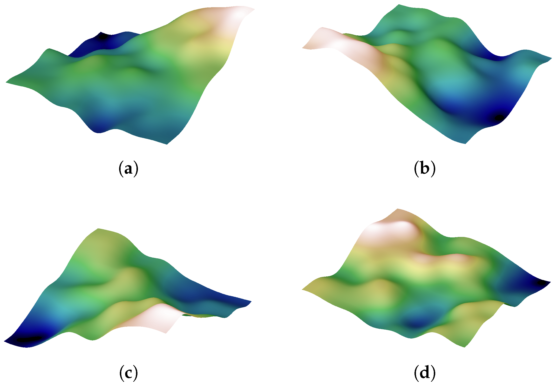
The DRL-DWA agent is trained using four parallel environments to accelerate the accumulation of experience and enhance exploration capabilities, ultimately improving the generalization performance of the model. Vectorized environments stack multiple independent environments with different terrains and obstacles into a single environment, effectively avoiding the agent’s overfitting to a specific scene, thereby achieving better performance in the testing phase. Four randomly generated terrain types, as shown in Figure 6, were used during the training process.

Equation (37) is used for training-scenario generation by utilizing Fractional Brownian motion (fBm) to fuse multi-layer Perlin noise [33] to simulate 3D uneven terrain [34]. In the equation, $PerlinNoise(x,y)$ represents Perlin noise, h represents the base elevation, $N_{layer}\in [1,\infty )$ controls the number of fusion layers, $b_p\in [0,1]$ is persistence, and $f_p\in [1,\infty )$ is frequency.

$$z(x,y)=h+\sum _{i=1}^{N_{layer}}{b}_p^i\times PerlinNoise(f_p^i\times x,f_p^i\times y)$$

(37)

In this paper, the parameters were set as $h=0,b_p=0.5$, and $f_p=1$.

4.3. Testing Scenarios and Evaluation Metrics

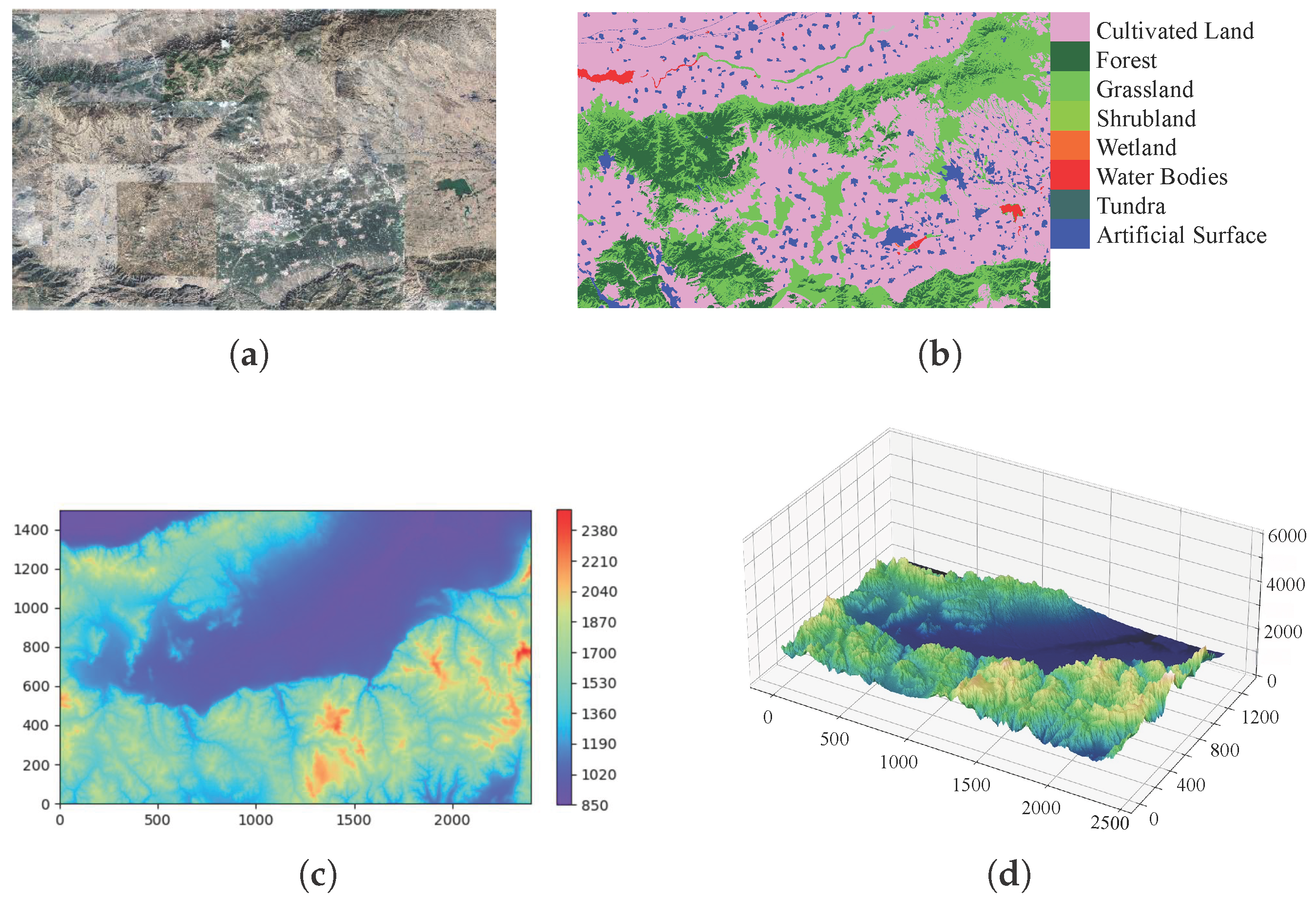
To ensure that the simulation environments reflect realistic off-road characteristics, we utilized NASA’s global Digital Elevation Model (DEM) dataset as the base terrain source. A $72\mathrm{km}\times 45\mathrm{km}$ region in Shanxi, China $({114}^{\circ }\mathrm{E},{40}^{\circ }\mathrm{N};{114}^{\circ }{51}^{\prime }\mathrm{E},{40}^{\circ }{27}^{\prime }\mathrm{N})$, was selected, and four $1\mathrm{km}\times 1\mathrm{km}$ subregions were extracted. Each subregion was interpolated to a $0.1\mathrm{m}\times 0.1\mathrm{m}$ grid using bicubic interpolation to obtain high-resolution elevation data that preserve natural slope variations. The corresponding satellite imagery, surface coverage, and DEM maps are shown in Figure 7, while the extracted results on real terrains are presented in Figure 9.

The effectiveness of the proposed method is assessed through the following four scenarios: a $1000\times 1000{\mathrm{m}}^2$ low elevation scenario with few obstacles and a maximum elevation gain of less than $100\mathrm{m}$; a $1000\times 1000{\mathrm{m}}^2$ medium elevation scenario with few obstacles and an elevation gain between 100–$200\mathrm{m}$; a $1000\times 1000{\mathrm{m}}^2$ high elevation scenario with few obstacles and a maximum elevation gain greater than $200\mathrm{m}$; and a $1000\times 1000{\mathrm{m}}^2$ scenario with numerous obstacles of different sizes.

The proposed method is evaluated against existing approaches using the following performance metrics:

• Success rate—The percentage of trials in which the UGV successfully navigates to the target while avoiding obstacles and restricted zones.
• Average trajectory length—The average distance traveled by the UGV from the start to the target, calculated across successful trials.
• Average travel time—The total time traveled by the UGV from the start to the target, averaged over the number of successful trials.
• Average elevation gradient—The elevation gradient encountered by the UGV along its trajectory, averaged over the successful trials.

4.4. Analysis and Comparison

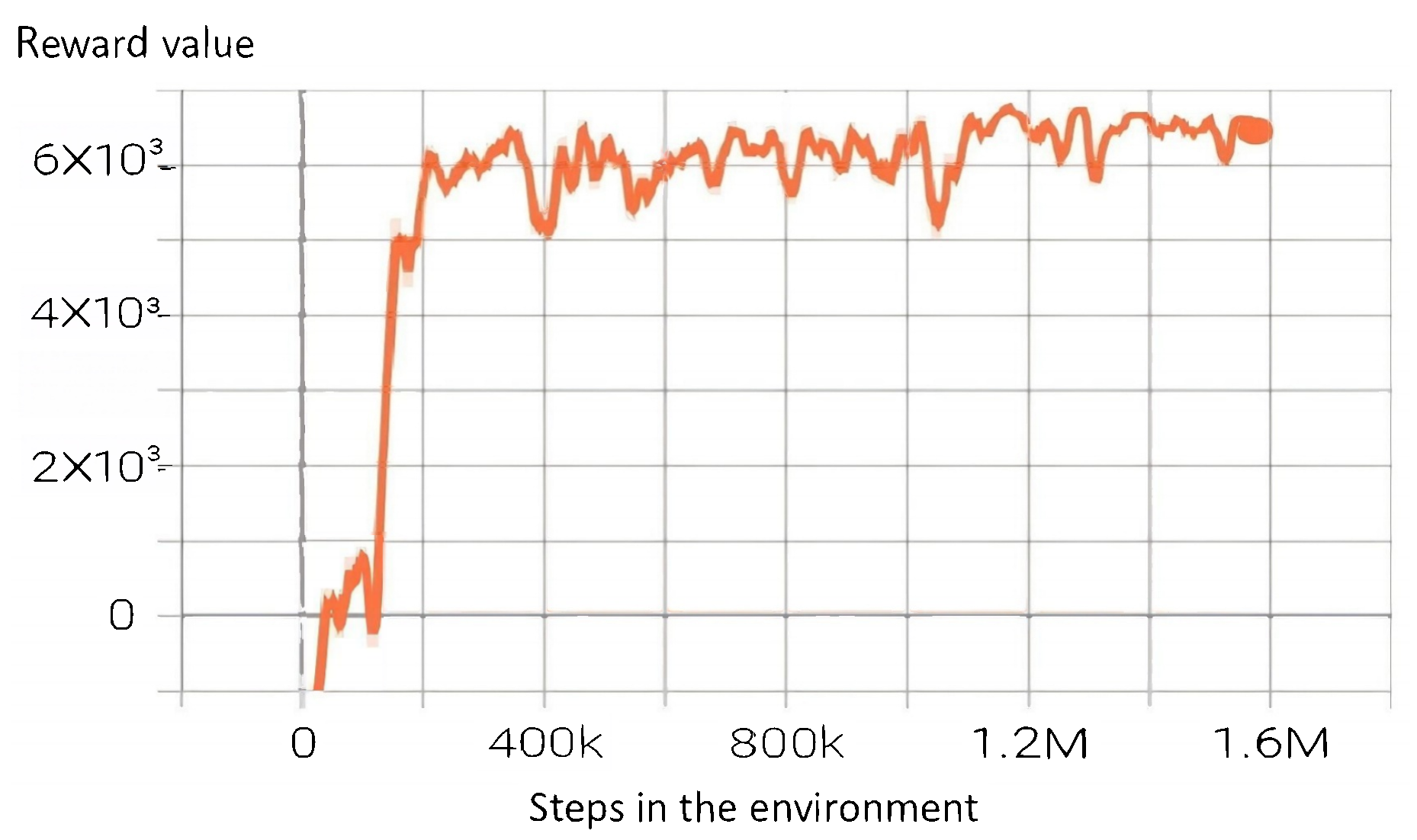
Figure 8 illustrates the policy’s reward progression during training. The reward curve exhibits oscillations due to task complexity but stabilizes after approximately 300,000 training steps as the policy converges.

We evaluate the proposed algorithm’s navigation performance against three baseline methods. Approach 1 is the dynamic window approach (DWA) proposed in [11]. Approach 2 is the ego-graph method proposed in [35], where the trajectories are generated by sets of steering velocity commands. Approach 3 is the improved DWA based on Q-learning proposed in [36]. It is worth noting that we add a global path planner based on D* Lite to [36] to facilitate better comparison (DWA-RL with D* Lite). Finally, the proposed method and the three baseline approaches are evaluated using the aforementioned metrics in different environments.

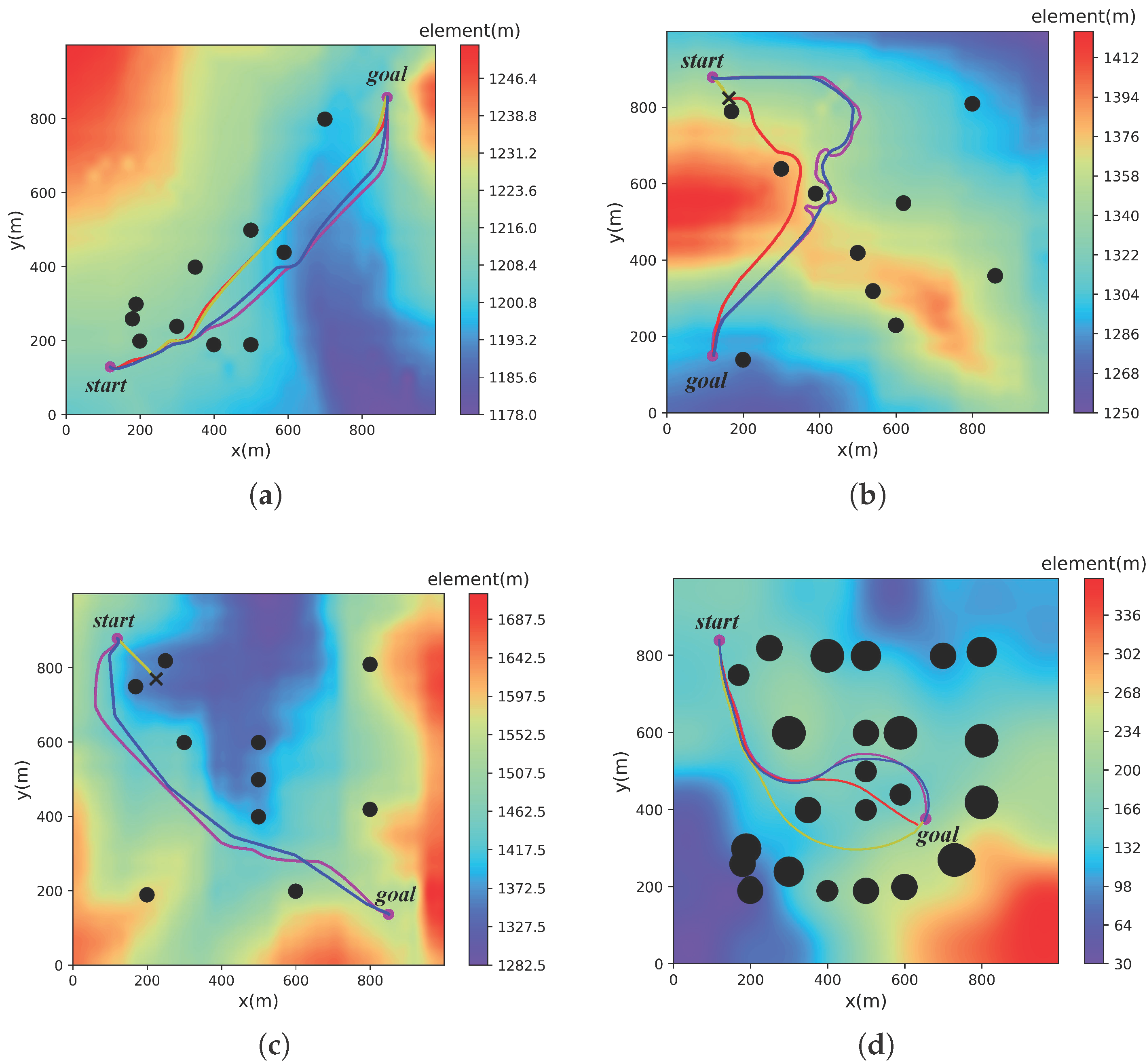
The evaluation uses 100 randomly generated start–goal position pairs, assuming that both the start and goal locations are traversable. A randomly selected set of simulation results depicting different scenarios is illustrated in Figure 9. It is evident that the proposed method generates paths that adeptly avoid obstacles. Furthermore, leveraging energy cost and elevation gradient, the planned paths tend to circumvent areas with significant surface fluctuations.

The simulation statistics are presented in

Table 1. Comparison of the proposed algorithm versus other methods on multiple evaluation metrics in different situations.

Scenarios	Method	Success Rate (%)	Average Trajectory Length (m)	Average Traveled Time (s)	Average Elevation Gradient
Low Elevation	DWA [11]	85	1364.34	132.64	1.79
	Ego-graph Method [35]	88	1357.76	132.93	1.74
	DWA-RL with D* Lite [36]	94	1398.54	133.21	1.68
	Proposed	94	1423.65	129.84	1.66
Medium Elevation	DWA [11]	72	1085.98	139.84	3.46
	Ego-graph Method [35]	69	1126.63	147.53	3.25
	DWA-RL with D* Lite [36]	79	1294.26	143.28	3.03
	Proposed	82	1320.21	143.57	2.98
High Elevation	DWA [11]	31	1259.32	142.17	4.06
	Ego-graph Method [35]	39	1243.65	143.25	3.82
	DWA-RL with D* Lite [36]	53	1298.43	152.14	3.46
	Proposed	59	1306.42	150.34	3.31
Numerous Obstacles	DWA [11]	54	775.41	97.32	1.95
	Ego-graph Method [35]	55	754.54	90.43	1.87
	DWA-RL with D* Lite [36]	70	794.02	88.65	1.80
	Proposed	71	802.82	89.01	1.78

. It is observed that as the elevation gain increases, the path planning success rate decreases for all methods. However, the proposed method exhibits the highest success rate and the lowest average elevation gradient across four different experimental environments. This is attributed to our method being guided by the least-cost global path while considering the elevation gradient information in local path planning. These findings suggest that the proposed algorithm exhibits good generalization ability in diverse off-road environments. Conversely, both the DWA and ego-graph-based methods are more susceptible to becoming trapped in local optima due to the absence of global path guidance. Additionally, the fixed parameter set of the DWA results in the UGV demonstrating the same navigation preference regardless of the situation, thereby leading to subpar performance.

The proposed DRL-DWA method is guided by an energy-efficient global path and incorporates the elevation gradient into the reinforcement learning reward function. Consequently, the planned paths tend to bypass areas with large surface fluctuations. The results in Table 1 validate that the proposed method has the lowest average elevation gradient among all compared approaches. Meanwhile, the average trajectory length increases by only 4.51%, while the average travel time decreases by 0.55% compared with the baselines. This indicates that the slightly longer paths are smoother and more dynamically feasible, allowing the UGV to maintain a higher average speed with fewer stops and turns. Hence, the performance improvement in stability and energy efficiency outweighs the minor trade-off in distance.

4.5. Formation Path Planning

To validate the effectiveness of the above formation control algorithm, Python 3 is used to simulate the formation algorithm. The simulation is conducted in two parts: linear trajectory simulation and circular trajectory simulation.

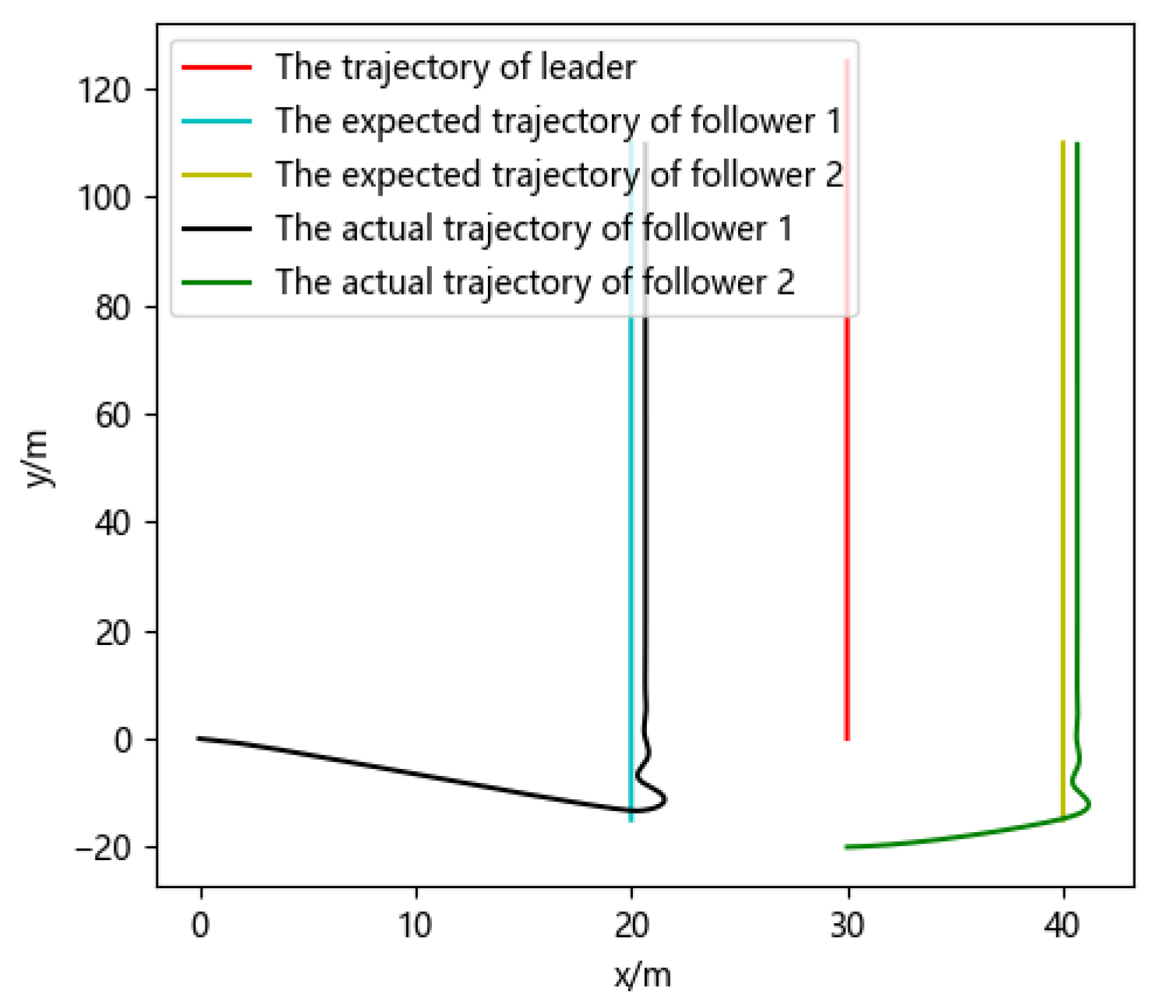
As shown in Figure 10, the linear trajectory simulation environment is a rectangular area of 50 m × 120 m. The starting coordinates of the leader are $(30,0)$, and the starting coordinates of follower 1 and follower 2 are $(0,0)$ and $(30,-20)$, respectively. The leader moves in a straight line at a linear speed of 0.5 m/s. The two followers follow the leader in a triangular formation using the above formation control algorithm.

Figure 11 shows the ideal and actual errors of follower 1 and follower 2 in the straight trajectory simulation. It is observed from the figure that the error is large at the beginning because the distance between the follower and the virtual UGV is very far. As the formation control algorithm continues to work, the followers quickly converge to the ideal trajectory and then continue to maintain the formation and move forward along the straight trajectory.

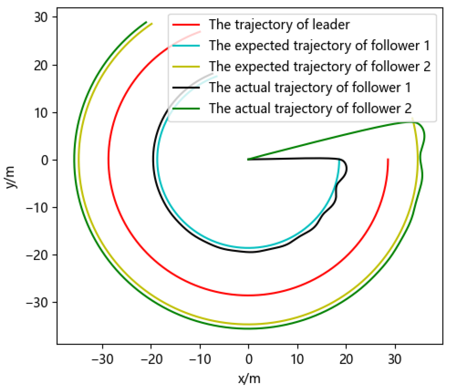
The circular trajectory simulation environment is a square area of 80 m × 80 m. The starting coordinates of the leader are $(28.7,0)$, and the starting coordinates of follower 1 and follower 2 are both $(0,0)$. The leader performs uniform circular motion at a linear velocity of 0.5 m/s and an angular velocity of ${\displaystyle \frac{\pi }{180}}$ rad/s. The two followers follow the leader in a triangular formation using the above formation control algorithm.

The expected and actual trajectories of the leader and the followers in the formation control simulation are shown in Figure 12. Follower 1 and follower 2 move to the ideal distance and angle with the leader through the formation control algorithm to form a triangular formation and can also maintain the formation well in the subsequent circular motion process.

Figure 13 shows the ideal and actual errors of follower 1 and follower 2 in the circular trajectory simulation. It is observed from the figure that the error is large at the beginning because the distance between the follower and the virtual UGV is very far. As the formation control algorithm continues to work, the follower quickly converges to the ideal trajectory and then continues to maintain the formation and move forward along the ideal trajectory.

During both linear and circular trajectory experiments, the steady-state formation errors remained within 2.5 m in distance and 3rad in orientation, demonstrating stable tracking performance. In the off-road terrain test, the proposed DRL-DWA-based formation maintained the desired triangular configuration while avoiding collisions and adapting to elevation changes, confirming its robustness and coordination capability.

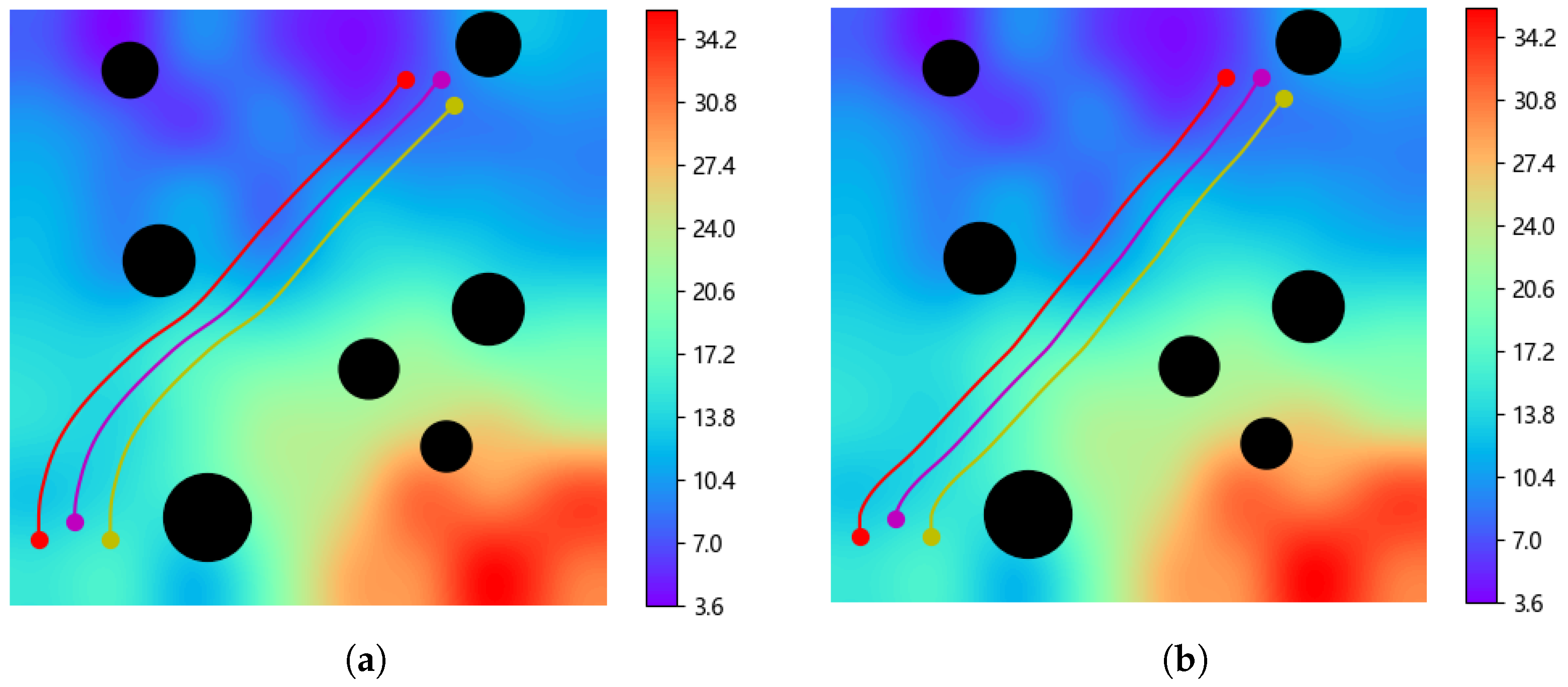
To validate the effectiveness of the proposed UGV formation path planning algorithm on off-road terrain, simulations are performed on real terrain data. The simulation environment is a square area of 150 m × 150 m. The terrain is relatively flat in the northwest direction, whereas the southeast region exhibits more pronounced elevation variations due to higher elevation. The leader and followers form a triangular formation at the initial moment, and the formation trajectory is shown in Figure 14. Among them, the magenta trajectory is the leader’s trajectory, the red and yellow trajectories are the followers’ trajectories, and the black circles are randomly generated obstacles. The leader uses the DRL-DWA-based path algorithm proposed in this paper to complete the navigation task. The followers track the leader according to the leader–follower method guided by the position of the virtual UGV. In addition, the leader and the followers form a triangular formation and move from the southwest to the northeast on the map, crossing the off-road terrain together while avoiding obstacles and avoiding internal collisions.

Figure 14b shows the DWA-based formation trajectory. This conventional approach, lacking off-road environment adaptation, prioritizes minimal path length over terrain considerations, resulting in trajectories through significant elevation variations. The proposed method takes into account information such as energy cost and elevation gradient so that the UGV formation can bypass the steep terrain areas in the map, thereby reducing energy consumption and improving the success rate of navigation.

5. Conclusions

This paper presents a novel approach for vehicle path planning in off-road environments, based on deep reinforcement learning and DWA. First, we propose a hierarchical path planning scheme to incorporate the pre-planned global path based on D* Lite into local path planning. Second, we combine DRL and DWA to address their respective limitations. Specifically, the weighting factors of the DWA evaluation functions are adaptively adjusted by the DRL network, and the final optimal control velocities are calculated by DWA, ensuring dynamic feasibility. Then, we expand the single UGV into a multi-UGV system and realize formation control through the leader–follower method. Finally, we evaluate the proposed algorithm against existing navigation methods using real-world terrain data, demonstrating that it enhances the planning success rate and reduces the average elevation gradient. Although the proposed DRL-DWA framework shows good performance, its current validation is limited to small-scale formations, and the conservative avoidance rule may reduce efficiency in dense obstacles. In addition, the DRL module depends on the training setup and may require retuning for new terrains. Future work will address these limitations and focus on validating the proposed algorithm on a physical vehicle in real-world off-road environments to further demonstrate its practicality.

References

1. Gan, X.; Huo, Z.; Li, W. DP-A*: For Path Planing of UGV and Contactless Delivery. IEEE Trans. Intell. Transp. Syst. 2023, 25, 907–919. [Google Scholar] [CrossRef]
2. Park, C.; Park, J.S.; Manocha, D. Fast and bounded probabilistic collision detection for high-DOF trajectory planning in dynamic environments. IEEE Trans. Autom. Sci. Eng. 2018, 15, 980–991. [Google Scholar] [CrossRef]
3. Liu, C.; Zhang, S.; Akbar, A. Ground feature oriented path planning for unmanned aerial vehicle mapping. IEEE J. Sel. Top. Appl. Earth Obs. Remote Sens. 2019, 12, 1175–1187. [Google Scholar] [CrossRef]
4. Waibel, G.G.; Löw, T.; Nass, M.; Howard, D.; Bandyopadhyay, T.; Borges, P.V.K. How rough is the path? Terrain traversability estimation for local and global path planning. IEEE Trans. Intell. Transp. Syst. 2022, 23, 16462–16473. [Google Scholar] [CrossRef]
5. Koenig, S.; Likhachev, M.; Furcy, D. Lifelong planning A*. Artif. Intell. 2004, 155, 93–146. [Google Scholar] [CrossRef]
6. Koenig, S.; Likhachev, M. Fast replanning for navigation in unknown terrain. IEEE Trans. Robot. 2005, 21, 354–363. [Google Scholar] [CrossRef]
7. Karaman, S.; Frazzoli, E. Sampling-based algorithms for optimal motion planning. Int. J. Robot. Res. 2011, 30, 846–894. [Google Scholar] [CrossRef]
8. Gammell, J.D.; Srinivasa, S.S.; Barfoot, T.D. Informed RRT: Optimal sampling-based path planning focused via direct sampling of an admissible ellipsoidal heuristic. In Proceedings of the 2014 IEEE/RSJ International Conference on Intelligent Robots and Systems, Chicago, IL, USA, 14–18 September 2014; pp. 2997–3004. [Google Scholar]
9. Katrakazas, C.; Quddus, M.; Chen, W.H.; Deka, L. Real-time motion planning methods for autonomous on-road driving: State-of-the-art and future research directions. Transp. Res. Part C Emerg. Technol. 2015, 60, 416–442. [Google Scholar] [CrossRef]
10. Hu, J.; Hu, Y.; Lu, C.; Gong, J.; Chen, H. Integrated path planning for unmanned differential steering vehicles in off-road environment with 3D terrains and obstacles. IEEE Trans. Intell. Transp. Syst. 2021, 23, 5562–5572. [Google Scholar] [CrossRef]
11. Fox, D.; Burgard, W.; Thrun, S. The dynamic window approach to collision avoidance. IEEE Robot. Autom. Mag. 1997, 4, 23–33. [Google Scholar] [CrossRef]
12. Xu, X.; Cai, P.; Ahmed, Z.; Yellapu, V.S.; Zhang, W. Path planning and dynamic collision avoidance algorithm under COLREGs via deep reinforcement learning. Neurocomputing 2022, 468, 181–197. [Google Scholar] [CrossRef]
13. Francis, A.; Faust, A.; Chiang, H.T.L.; Hsu, J.; Kew, J.C.; Fiser, M.; Lee, T.W.E. Long-range indoor navigation with prm-rl. IEEE Trans. Robot. 2020, 36, 1115–1134. [Google Scholar] [CrossRef]
14. Sathyamoorthy, A.J.; Liang, J.; Patel, U.; Guan, T.; Chandra, R.; Manocha, D. Densecavoid: Real-time navigation in dense crowds using anticipatory behaviors. In Proceedings of the 2020 IEEE International Conference on Robotics and Automation (ICRA), Paris, France, 31 May–31 August 2020; pp. 11345–11352. [Google Scholar]
15. Zhu, Y.; Mottaghi, R.; Kolve, E.; Lim, J.J.; Gupta, A.; Fei-Fei, L.; Farhadi, A. Target-driven visual navigation in indoor scenes using deep reinforcement learning. In Proceedings of the 2017 IEEE International Conference on Robotics and Automation (ICRA), Singapore, 29 May–3 June 2017; pp. 3357–3364. [Google Scholar]
16. Zhou, S.; Xi, J.; McDaniel, M.W.; Nishihata, T.; Salesses, P.; Iagnemma, K. Self-supervised learning to visually detect terrain surfaces for autonomous robots operating in forested terrain. J. Field Robot. 2012, 29, 277–297. [Google Scholar] [CrossRef]
17. Shan, Y.; Fu, Y.; Chen, X.; Lin, H.; Zhang, Z.; Lin, J.; Huang, K. LiDAR Based Traversable Regions Identification Method for Off-Road UGV Driving. IEEE Trans. Intell. Veh. 2024, 9, 3544–3557. [Google Scholar] [CrossRef]
18. Guastella, D.C.; Muscato, G. Learning-based methods of perception and navigation for ground vehicles in unstructured environments: A review. Sensors 2020, 21, 73. [Google Scholar] [CrossRef] [PubMed]
19. Nguyen, A.; Nguyen, N.; Tran, K.; Tjiputra, E.; Tran, Q.D. Autonomous navigation in complex environments with deep multimodal fusion network. In Proceedings of the 2020 IEEE/RSJ International Conference on Intelligent Robots and Systems (IROS), Las Vegas, NV, USA, 25–29 October 2020; pp. 5824–5830. [Google Scholar]
20. Mayuku, O.; Surgenor, B.W.; Marshall, J.A. A self-supervised near-to-far approach for terrain-adaptive off-road autonomous driving. In Proceedings of the 2021 IEEE International Conference on Robotics and Automation (ICRA), Xi’an, China, 30 May–5 June 2021; pp. 14054–14060. [Google Scholar]
21. Zhang, K.; Niroui, F.; Ficocelli, M.; Nejat, G. Robot navigation of environments with unknown rough terrain using deep reinforcement learning. In Proceedings of the 2018 IEEE International Symposium on Safety, Security, and Rescue Robotics (SSRR), Philadelphia, PA, USA, 6–8 August 2018; pp. 1–7. [Google Scholar]
22. Josef, S.; Degani, A. Deep reinforcement learning for safe local planning of a ground vehicle in unknown rough terrain. IEEE Robot. Autom. Lett. 2020, 5, 6748–6755. [Google Scholar] [CrossRef]
23. Weerakoon, K.; Sathyamoorthy, A.J.; Patel, U.; Manocha, D. Terp: Reliable planning in uneven outdoor environments using deep reinforcement learning. In Proceedings of the 2022 International Conference on Robotics and Automation (ICRA), Philadelphia, PA, USA, 23–27 May 2022; pp. 9447–9453. [Google Scholar]
24. Zhu, L.; Huang, K.; Wang, Y.; Hu, Y. A Multi-Objective Path Planning Framework in Off-Road Environments Based on Deep Reinforcement Learning. IEEE Trans. Intell. Transp. Syst. 2025, 1–19. [Google Scholar] [CrossRef]
25. Fan, J.; Fan, L.; Ni, Q.; Wang, J.; Liu, Y.; Li, R.; Wang, Y.; Wang, S. Perception and Planning of Intelligent Vehicles Based on BEV in Extreme Off-Road Scenarios. IEEE Trans. Intell. Veh. 2024, 9, 4568–4572. [Google Scholar] [CrossRef]
26. Patel, U.; Kumar, N.K.S.; Sathyamoorthy, A.J.; Manocha, D. Dwa-rl: Dynamically feasible deep reinforcement learning policy for robot navigation among mobile obstacles. In Proceedings of the 2021 IEEE International Conference on Robotics and Automation (ICRA), Xi’an, China, 30 May–5 June 2021; pp. 6057–6063. [Google Scholar]
27. Langer, D.; Rosenblatt, J.; Hebert, M. A behavior-based system for off-road navigation. IEEE Trans. Robot. Autom. 1994, 10, 776–783. [Google Scholar] [CrossRef]
28. Zhang, Y.; Li, C. On Hierarchical Path Planning Based on Deep Reinforcement Learning in Off- Road Environments. In Proceedings of the 2024 10th International Conference on Automation, Robotics and Applications (ICARA), Athens, Greece, 22–24 February 2024; pp. 461–465. [Google Scholar]
29. Rowe, N.C.; Ross, R.S. Optimal grid-free path planning across arbitrarily-contoured terrain with anisotropic friction and gravity effects. IEEE Trans. Robot. Autom. 1990, 6, 540–553. [Google Scholar] [CrossRef]
30. Ganganath, N.; Cheng, C.T.; Chi, K.T. A constraint-aware heuristic path planner for finding energy-efficient paths on uneven terrains. IEEE Trans. Ind. Inform. 2015, 11, 601–611. [Google Scholar] [CrossRef]
31. Thrun, S.; Littman, M.L. Reinforcement learning: An introduction. AI Mag. 2000, 21, 103. [Google Scholar]
32. Schulman, J.; Wolski, F.; Dhariwal, P.; Radford, A.; Klimov, O. Proximal policy optimization algorithms. arXiv 2017, arXiv:1707.06347. [Google Scholar] [CrossRef]
33. Perlin, K. An image synthesizer. ACM Siggraph Comput. Graph. 1985, 19, 287–296. [Google Scholar] [CrossRef]
34. Jain, A.; Sharma, A.; Rajan. Adaptive & Multi-Resolution Procedural Infinite Terrain Generation with Diffusion Models and Perlin Noise. In Proceedings of the Thirteenth Indian Conference on Computer Vision, Graphics and Image Processing, Gandhinagar, India, 8–10 December 2022; pp. 1–9. [Google Scholar]
35. Lacaze, A.; Moscovitz, Y.; DeClaris, N.; Murphy, K. Path planning for autonomous vehicles driving over rough terrain. In Proceedings of the 1998 IEEE International Symposium on Intelligent Control (ISIC) Held Jointly with IEEE International Symposium on Computational Intelligence in Robotics and Automation (CIRA) Intell, Gaithersburg, MD, USA, 17 September 1998; pp. 50–55. [Google Scholar]
36. Chang, L.; Shan, L.; Jiang, C.; Dai, Y. Reinforcement based mobile robot path planning with improved dynamic window approach in unknown environment. Auton. Robot. 2021, 45, 51–76. [Google Scholar] [CrossRef]
Figure 1. DRL-DWA’s overall system architecture.
Applsci 15 12212 g001
Figure 2. Convert raster data to a graph with eight-connected neighborhoods.
Applsci 15 12212 g002
Figure 3. Illustration of a global path planning scenario. The D* Lite algorithm generates the optimal trajectory represented by the red polyline. The nodes ( P 1 , P 2 , , P i , ) selected by the global path serve as the waypoints for the local path planning. r a d i u s is the effective radius of each waypoint. When the vehicle comes within r a d i u s of the current waypoint, the next waypoint is selected as the sub-target of local path planning.
Applsci 15 12212 g003
Figure 4. The network architecture of our DRL network.
Applsci 15 12212 g004
Figure 5. Leader–follower formation motion model.
Applsci 15 12212 g005
Figure 6. Four representative terrain types used for training: (a) Low-frequency terrain; (b) Medium-frequency terrain; (c) High-frequency terrain; (d) Mixed-frequency terrain.
Applsci 15 12212 g006
Figure 7. Digital elevation model of the selected area. (a) Satellite image. (b) Surface coverage. (c) Two-dimensional diagram of DEM data. (d) Three-dimensional diagram of DEM data.
Applsci 15 12212 g007
Figure 8. The horizontal axis represents the policy’s training steps, while the vertical axis displays the moving average reward per 100 episodes.
Applsci 15 12212 g008
Figure 9. Comparison of paths driven by the proposed algorithm (magenta), the dynamic window approach (yellow), the ego-graph method (red), and DWA-RL with D* Lite (blue). The black solid circles represent obstacles: (a) Low elevation. (b) Medium elevation. (c) High elevation. (d) Numerous obstacles.
Applsci 15 12212 g009
Figure 10. Linear trajectory simulation result.
Applsci 15 12212 g010
Figure 11. Errors between the ideal and actual followers in the linear trajectory simulation: (a) Follower 1. (b) Follower 2.
Applsci 15 12212 g011
Figure 12. Circular trajectory simulation result.
Applsci 15 12212 g012
Figure 13. Error between the ideal and actual followers in the circular trajectory simulation: (a) Follower 1. (b) Follower 2.
Applsci 15 12212 g013
Figure 14. Comparison of formation trajectories based on different navigation algorithms: (a) Formation trajectory based on DRL-DWA. (b) Formation trajectory based on DWA.
Applsci 15 12212 g014