Life Cycle Cost Analysis of a Biomass-Driven ORC Cogeneration System for Medical Cannabis Greenhouse Cultivation

Abstract

Medical cannabis cultivation requires substantial energy for heating, lighting, and climate control. This study evaluates the economic feasibility of an innovative biomass-fired micro-CHP system in a greenhouse facility for medicinal cannabis cultivation. The system comprises an 80 kW_th boiler retrofitted for biomass and a 7 kW_el ORC engine and is assessed against a diesel-boiler Business-As-Usual (BAU) benchmark. Thermal load simulations for two growing periods (1 March–30 June and 1 September–30 December) estimate an annual heating demand of 91,065.20 kWh_th. The micro-CHP system delivers 8195.87 kWh_el per year, exceeding the greenhouse’s 7839.90 kWh_el consumption. Over a 30-year lifespan at a 7% discount rate, Life Cycle Costing yields EUR 196,421.33 for micro-CHP versus EUR 229,468.46 for BAU, a 14.4% reduction. Under all-equity financing, the project achieves an NPV of EUR 59,591.88, IRR of 27.32%, and a DPBP of 12.1 years; with 70% debt financing, NPV rises to EUR 61,211.39 and DPBP shortens to 10.5 years. Levelized Cost of Energy (LCOE) and Heat (LCOH) are EUR 0.122 per kWh_el and EUR 0.062 per kWh_th, respectively. While the LCOE is below the Greek and EU non-household averages (EUR 0.1578 and EUR 0.1515 per kWh_el), the LCOH exceeds the corresponding heat price benchmarks (EUR 0.0401 and EUR 0.0535 per kWh_th). These results indicate that, in the modeled context, biomass-ORC cogeneration can be a financially attractive and lower-carbon option for medicinal cannabis greenhouse operations.

1. Introduction

1.1. Medical Cannabis Cultivation

Cannabis (Cannabis sativa L.) is a plant primarily known for its psychoactive properties, which are caused by tetrahydrocannabinol (THC). THC is the primary psychoactive compound and the most recognizable, but beyond this well-known facet, the therapeutic potential of cannabis has emerged as a global focus, placing the species among the most discussed in botanical and medical sciences [1]. In recent years, cannabis has raised public awareness in many countries worldwide about its medical uses, as an expanding body of research and regulatory shifts has underscored the plant’s value for therapeutic purposes. This has subsequently led to a number of jurisdictions either decriminalizing cannabis or legalizing it for medical use, with some moving toward full legalization [2,3]. As societal and legislative landscapes continue to evolve and public acceptance grows, a dedicated cannabis industry has emerged to meet consumer demand and preferences, such as demand for cannabis-based medicines [4].

In March of 2018, Greece introduced Law 4523/2018, which regulates the production and processing of medical cannabis. This law was applied due to the desire to revitalize the crop industry and to trade in cannabis products [5]. For the granting of approval for installation and authorization, the applicant must submit documents for all stages (from cultivation to processing and production of final medical cannabis products). On the basis of legislation, the cultivation will take place under greenhouse or indoor conditions [6]. This legal requirement aligns with a broader modernization trend in agriculture toward controlled-environment agriculture (CEA). In practice, high-value cannabis is primarily grown in controlled settings using year-round production schedules, soilless systems, and data-driven climate control [7]. Recent analyses identify greenhouses as a means for continuous production, precise environmental management, and improved resource efficiency [8,9]. At the same time, greenhouse and high-tunnel studies on cannabis/hemp demonstrate that protected cultivation can improve crop uniformity and influence cannabinoid and aromatic profiles compared with open-field systems, which helps explain why medicinal cannabis projects gravitate to greenhouses even when costs are higher [10,11]. In this sense, the legal framework does not create an isolated practice but rather situates medicinal cannabis production within the ongoing move toward greenhouse-based CEA.

1.2. Energy Use in Medicinal Cannabis Greenhouses

Greenhouses, particularly in Mediterranean climates, are widely used for crop cultivation due to their ability to regulate environmental conditions and enhance productivity [12]. They are, however, energy-intensive systems, especially when used for high-demand crops like cannabis. Heating in conventional greenhouses is typically achieved through hot air or hot water systems, and energy use has become a growing concern due to rising costs and environmental impacts. This has driven increased interest in renewable energy sources (RES) integration to reduce reliance on non-renewable sources [13].

Legalized cannabis cultivation in various regions is a particularly energy-intensive greenhouse application. Basic energy consumption includes lighting, dehumidification, heating, and cooling; yet recent reviews and program reports highlight a persistent lack of standardized, publicly available energy-use data for cannabis cultivation, particularly outside North America, underscoring the need for benchmarking and comparable metrics to support robust techno-economic and environmental analyses [14,15,16,17].

For illustration, cannabis cultivation accounted for 45.5% of Denver’s 1.2% year-over-year increase in electricity demand in 2014 [18], and in California, indoor cannabis uses about 3% of the state’s and 1% of the nation’s electricity [19]. Reported electricity intensity spans ~21.7 kWh_el·m⁻² for outdoor production to ~2820 kWh_el·m⁻² for indoor facilities, whereas greenhouse vegetables and flowers typically consume ~167–785 kWh_th·m⁻²·yr⁻¹ [20]. In indoor cannabis operations, HVAC and lighting commonly account for ~51% and ~38% of electricity use, respectively [19], while electricity represents only ~10–15% of total energy in conventional greenhouses [21]. Complementing these benchmarks, modeled U.S. indoor scenarios estimate total site energy at approximately 2.3–6.0 MWh·kg⁻¹ (1.8–4.6 MWh·kg⁻¹ of electricity, plus space-heating fuels of 0.47–1.47 MWh·kg⁻¹) [22]. Greenhouse compilations [23] report electricity productivity of approximately 0.68 g·kWh⁻¹ (i.e., 1.47 MWh of electricity per kg of dried flower) and heating fuel use around 552 kWh·m⁻²·yr⁻¹, noting that system boundaries vary across studies. European figures, though sparse, align with high energy demand under protected cultivation. A Portuguese medical cannabis greenhouse (15,000 m²) was estimated at ~2209 MWh·yr⁻¹ (~147 kWh·m⁻²·yr⁻¹), with HVAC and pumping totaling to ~87.5 kWh m⁻²·yr⁻¹ [24]. Moreover, a Dutch desk study calculates a direct energy requirement of ~2.12 kWh·g⁻¹ (~6366 kWh·m⁻²·yr⁻¹ under a stylized high-intensity regime), highlighting both the potential magnitude of loads and the current reliance on modeled estimates in Europe [25].

Cannabis cultivation progresses through three main stages—propagation (or seedling), vegetative, and flowering—each stage has distinct requirements for light, temperature, and humidity, which result in varying energy demands (

Table 1. Requirements for different stages of cannabis cultivation.

Cultivation Stage	Duration	Cultivation Stages’ Needs
		Lighting	Dehumidification	Cooling
Propagation	1–2 weeks	54–431 W·m−2, 18–24 h	Low	Low
Vegetative	2–6 weeks	161–753 W·m−2, 18 h	Medium	High
Flowering	6–11 weeks	40–70 W·m−2, 12 h	High	Very high

). The propagation stage typically lasts 1 to 2 weeks and involves low-intensity lighting (54–431 W·m⁻²) for 18 to 24 h per day. This stage accounts for less than 5% of total electricity consumption [26]. Optimal environmental conditions require a temperature range between 24 and 26 °C and relative humidity (RH) of 70–75%, which can be maintained using split air conditioning units [27]. The vegetative stage lasts 2–3 weeks in indoor setups (or 4 to 6 weeks in greenhouses), using medium-intensity lighting (161–753 W·m⁻²) for 18 h daily. This phase consumes approximately 30–40% of total electricity [26]. While metal halide (MH) and high-pressure sodium (HPS) lamps have been traditionally used, modern operations increasingly adopt LED or ceramic metal halide (CMH) lighting. Climate conditions during this stage are typically regulated with rooftop HVAC units. The flowering stage is the most energy-intensive, accounting for 50–65% of total electricity use. It lasts 7–11 weeks and requires 12 h of lighting per day, at an intensity of 40–70 W m⁻². Environmental control is maintained using rooftop HVAC systems and dehumidifiers to ensure proper temperature and humidity levels [26].

Facility type, of course, strongly influences energy use. As of 2017, 60% of U.S. legal cannabis electricity demand was from indoor operations and 37% from greenhouses. Energy costs in indoor cultivation can reach 20–50% of operating expenses, equating to roughly 1614 kWh·m⁻² per year. Despite the lower energy intensity of outdoor cultivation, indoor and greenhouse methods are favored for yield control and consistency. Consequently, utilities and planners must understand this load’s profile [28].

Incentivizing best practices, such as LED adoption, off-peak scheduling, and cogeneration solutions such as biomass-fired ORC systems, can reduce the energy footprint of cannabis greenhouses. Emerging regulations that mandate energy plans, monitoring, and reporting, alongside local policies, can foster efficiency, build consumption databases, and help set realistic energy use targets.

1.3. Micro-CHP (Combined Heat and Power) in Greenhouse Applications

Combined Heat and Power (CHP), or cogeneration, holds significant potential across a range of industries. Among them are greenhouses, one of the most energy-intensive segments of modern agriculture. CHP systems are already in use across several greenhouse complexes, particularly in the Netherlands, where they have shown high efficiency and flexibility. As Canova et al. [29] point out, cogeneration is widely recognized for its superior fuel efficiency compared to the separate production of heat and electricity.

Greenhouses, as a form of CEA, offer a way to optimize growing conditions year-round, providing high productivity while improving resource efficiency. They can achieve high yields while substantially reducing water consumption, land use, and chemical inputs. However, these benefits come with significant energy demands, particularly for heating, lighting, and ventilation, making energy efficiency a critical concern for long-term sustainability. In this context, CHP systems can generate electricity on-site while utilizing the resulting heat for immediate use, efficiently meeting the diverse energy needs of greenhouse operations. Compared to traditional setups that rely on grid electricity and separate boilers, CHP systems reduce energy losses and environmental impact [30]. They can also be paired with complementary technologies like absorption cooling or carbon capture and utilization (CCU), expanding their benefits even further.

In practice, CHP is already being used successfully in greenhouse cultivation, particularly in Northern European countries. These systems often supply electricity to the grid while using the heat and CO₂ byproducts to enhance the indoor environment [31]. When the on-site electricity demand is lower than the system’s output, excess power can be sold back to the grid, providing an additional income stream.

Beyond their operational benefits, CHP systems are increasingly seen as a strategic tool for reducing the carbon footprint of energy-intensive agricultural practices [32]. Their ability to improve efficiency, lower emissions, and integrate with existing greenhouse infrastructure makes them especially well-suited for sustainable greenhouse cultivation. A key challenge, however, lies in developing advanced CHP systems that can effectively integrate renewable energy sources and adapt to variable weather patterns, while maintaining a reliable balance between energy supply and demand [33].

The integration potential of micro-CHP systems with other RES-assisted and energy-efficient solutions has been shown to further enhance energy autonomy and sustainability. Moreover, continuous progress in fuel cell technology has motivated researchers and industry to consider adopting fuel cell-based micro-CHP systems as promising candidates for future sustainable energy solutions [34]. Hybrid micro-CHP systems that combine photovoltaic (PV) systems, battery storage, and predictive control algorithms can dynamically balance supply and demand, achieving near-zero grid dependency [35]. The coupling of photovoltaic–thermal (PVT) collectors with Stirling- and ORC-based micro-CHP units has also emerged as a promising configuration for residential and agricultural buildings, stably delivering power and heat even under variable solar conditions [36]. These configurations can anticipate energy fluctuations and ensure that the micro-CHP unit operates only when required, minimizing both operational costs and carbon emissions.

From a broader perspective, international experiences reflect the growing attention that micro-CHP technologies receive due to policy incentives and technological advances, which provide higher electrical efficiencies and lower CO₂ emissions compared to conventional boilers [37]. Studies on distributed renewable-based CHP systems have further shown that hybridizing with solar and wind power can meet up to 79% of community-level energy demand while reducing over 4000 tCO₂ annually [38]. The inclusion of biofuels such as biogas or biodiesel in CHP operation has also proven effective for reducing fossil fuel dependence and enhancing combustion performance [39].

The Organic Rankine Cycle (ORC) Technology

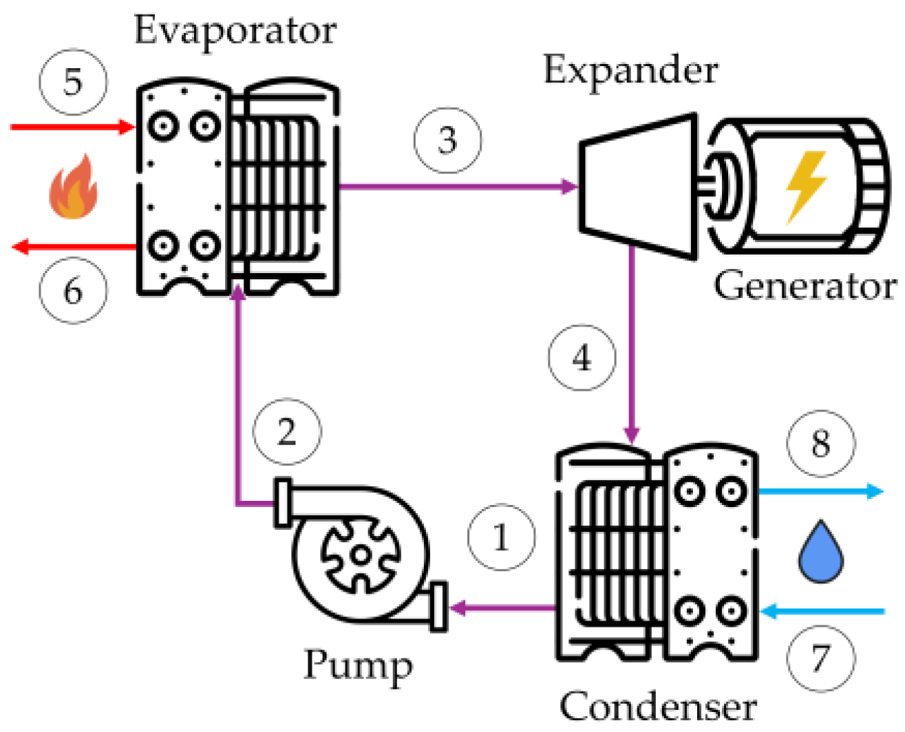
The organic Rankine cycle (ORC) is a closed thermodynamic process used for power generation. Although it follows the same basic principles as the Clausius–Rankine cycle, it uses organic working fluids instead of water or steam. The ORC exploits heat from a high-temperature source into mechanical work, while releasing excess heat to a cold sink, typically the environment. It is commonly applied for recovering energy from low-grade heat sources such as waste heat, solar power, geothermal energy, biomass, and hybrid systems [40]. The main components of a basic ORC system, namely the feed pump, evaporator, expander (or turbine), and condenser, are illustrated in Figure 1 [41]. The corresponding thermodynamic cycle comprises liquid compression (1–2), phase change in the evaporator (2–3), expansion in the expander or turbine (3–4), and condensation (4–1). The heat source and heat sink are finite thermal reservoirs, indicated by lines (5–6) and (7–8), respectively.

In commercial applications, for small-scale (up to a few tens of kW) and relatively small-scale (up to a few tens of kW) at low temperature (below 100–120 °C), the basic ORC setup (Figure 1) is almost exclusively used. With proper selection of working fluids for each application, the ORC can outperform the conventional water/steam Rankine cycle for waste heat recovery at temperatures up to 300 °C. This is mainly due to the lower critical temperatures of organic fluids, which allow for more efficient heat transfer and optimized system design [42]. The sustainability of the ORC technology is clearly demonstrated by the growing number of installations. Over the past decade, 759 installations have been completed, with an additional 63 currently under construction [43]. Nearly one-third of these installed systems (31.5%) are biomass-based.

1.4. Research Objectives and Scope

This study will investigate the economic feasibility of an innovative micro-CHP system, incorporating a biomass boiler and an ORC engine for a greenhouse facility intended for cultivating medicinal cannabis. Techno-economic metrics, such as Life Cycle Cost (LCC), Net Present Value (NPV), Discounted Payback Period (DPBP), and Internal Rate of Return (IRR), will be evaluated to determine the economic viability for a medicinal cannabis cultivator to invest in replacing the conventional system with the innovative micro-CHP configuration.

To this end, two main scenarios are analyzed. The first is the Business-As-Usual (BAU) scenario, in which the greenhouse relies exclusively on a diesel-fired boiler for heating and draws electricity from the grid. The second is the innovative micro-CHP (m-CHP) scenario, which features a boiler retrofitted for biomass combustion, integrated with an ORC engine for on-site power generation. In this setup, the ORC engine operates in parallel with the boiler, producing electricity whenever the boiler is active. In both scenarios, electricity consumption is supplied by the grid; however, in the m-CHP scenario, the electricity generated on-site is fed into the grid under a net metering arrangement. Following the simulation of the greenhouse’s thermal load profile, the corresponding thermal and electrical energy outputs of the m-CHP system are estimated.

2. Materials and Methods

2.1. Description of the Micro-CHP and Greenhouse Setup

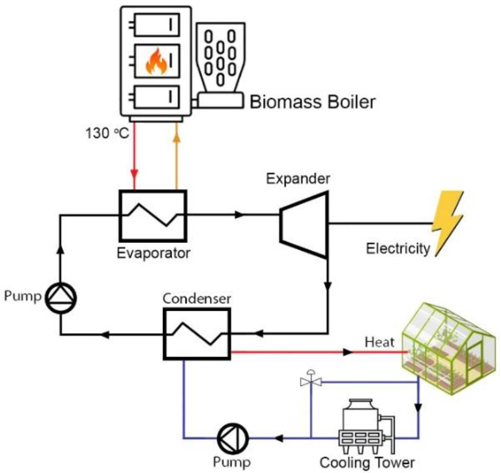
The study is based on the performance of an existing micro-CHP system installed at the Agricultural University of Athens (AUA). The system comprises (i) a fire-tube biomass boiler with modular, water-jacketed sections and (ii) an ORC unit for power generation, sized to meet the thermal requirements of a small greenhouse. As illustrated in Figure 2, the biomass boiler heats a glycol-based working fluid to 130 °C, providing up to 200 kW_th of thermal capacity. The heated working fluid then flows into the hot side of the ORC evaporator, where heat is transferred to the R1233zd(E) refrigerant. A single cooling loop condenses the refrigerant in the ORC condenser, and the rejected heat from this condenser is used to warm the greenhouse air.

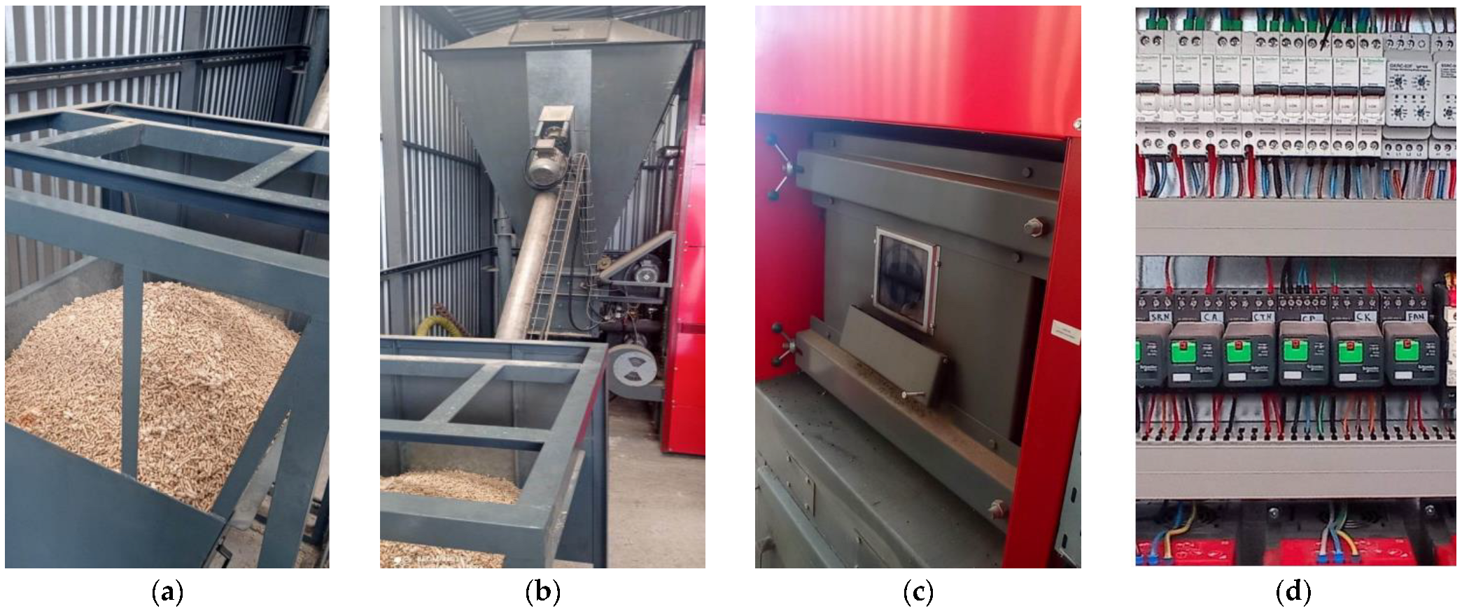
Figure 3 presents photographs of the biomass system components, including the storage hoppers, comprising the main silo and the smaller open tank, boiler, and the control panel, installed in a dedicated enclosure adjacent to the greenhouse. The biomass feedstock used consists of wood pellets that are commercially available in Greece, typically produced from debarked coniferous residues sourced domestically or from neighboring Balkan regions. These pellets are delivered in bulk over transport distances of approximately 100–150 km. From the open tank, pellets are moved to the feeder and then to the boiler’s combustion chamber by screw conveyors with stainless-steel blades, controlled by level-sensor readings. As a standardized market product, no on-site drying or special storage procedures are applied, apart from standard covered storage at the boiler facility to protect the pellets from moisture and weather exposure. The main technical specifications of the biomass boiler and fuel storage system are summarized in

Table 2. Main technical specifications of the biomass boiler and fuel storage system.

Specification	Value
Boiler efficiency	85%
Hopper volume (silo and open tank) [L]	5210.00
Boiler operating autonomy [h] a	~34

^a Considering biomass LHV and density of 5.2 kWh·kg⁻¹ and 0.6 kg·L⁻¹, respectively.

.

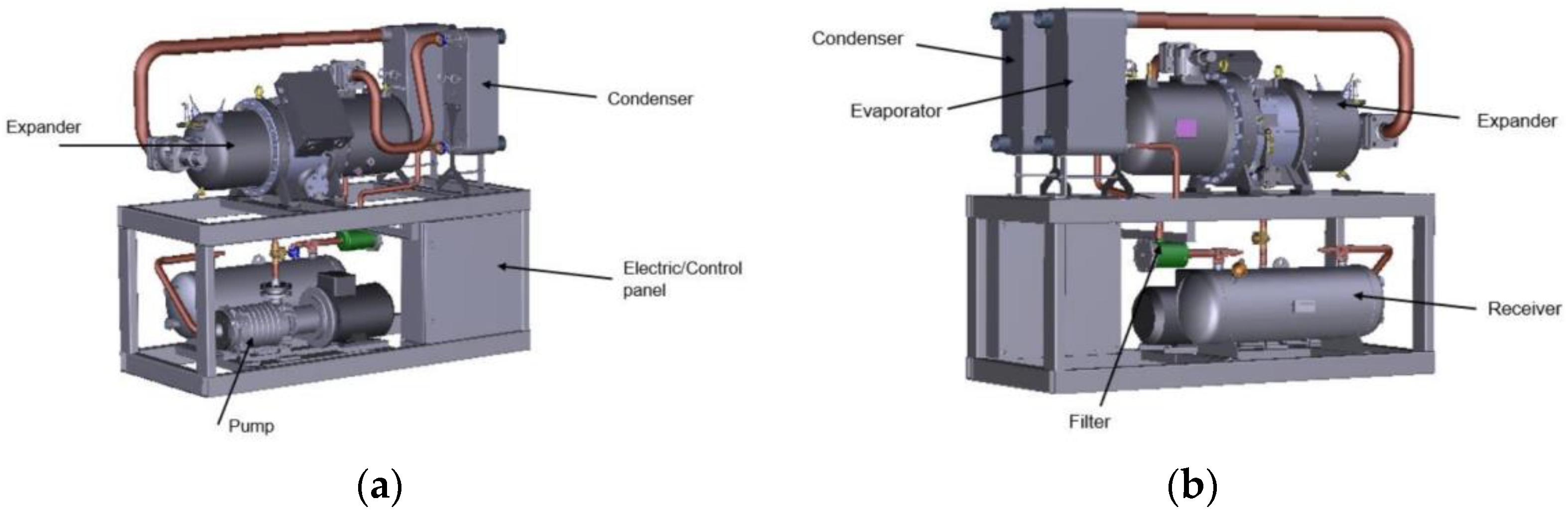
The ORC engine operates at fixed frequencies for both the pump (Freq_pu) and the expander (Freq_exp). The system achieves a maximum net electrical output (P_net,ORC) of 20.39 kW when the pump operates at 42.70 Hz and the expander at 60.00 Hz. Additional test data across various frequency settings for both components are presented in

Table A1. Experimental data on power generation of the ORC system at AUA.

Freqpu (Hz)	Freqexp (Hz)	Tcon,in (°C)	Pel,exp (kWel)	Pel,pu (kWel)	Pnet,ORC (kWel)
15	25	47.50	1.91	0.29	1.62
15	30	45.70	2.99	0.35	2.64
20	35	50.60	3.04	0.48	2.56
25	25	54.00	1.45	0.57	0.88
25	30	54.20	2.25	0.84	1.41
25	35	54.30	2.30	0.85	1.45
30	30	46.50	5.16	1.40	3.76
30	50	64.90	6.28	1.40	4.88
35	40	64.30	7.82	1.68	6.14
35	45	54.20	11.86	2.23	9.63
35	50	64.30	9.92	1.84	8.08
35	55	66.10	11.57	2.03	9.54
40	50	64.40	14.46	2.60	11.86
40	60	64.30	15.60	2.85	12.75
45	60	64.20	24.82	3.89	20.93

(Appendix A). The recorded parameters include the condenser inlet temperature (T_con,in in °C), the expander’s electrical power output (P_el,exp in kW), and the pump’s electrical power consumption (P_el,pu in kW). Figure 4 illustrates 3D models of the ORC unit designed to produce 20 kW_el, showing its primary cycle components—namely the condenser, compressor, evaporator, and expander.

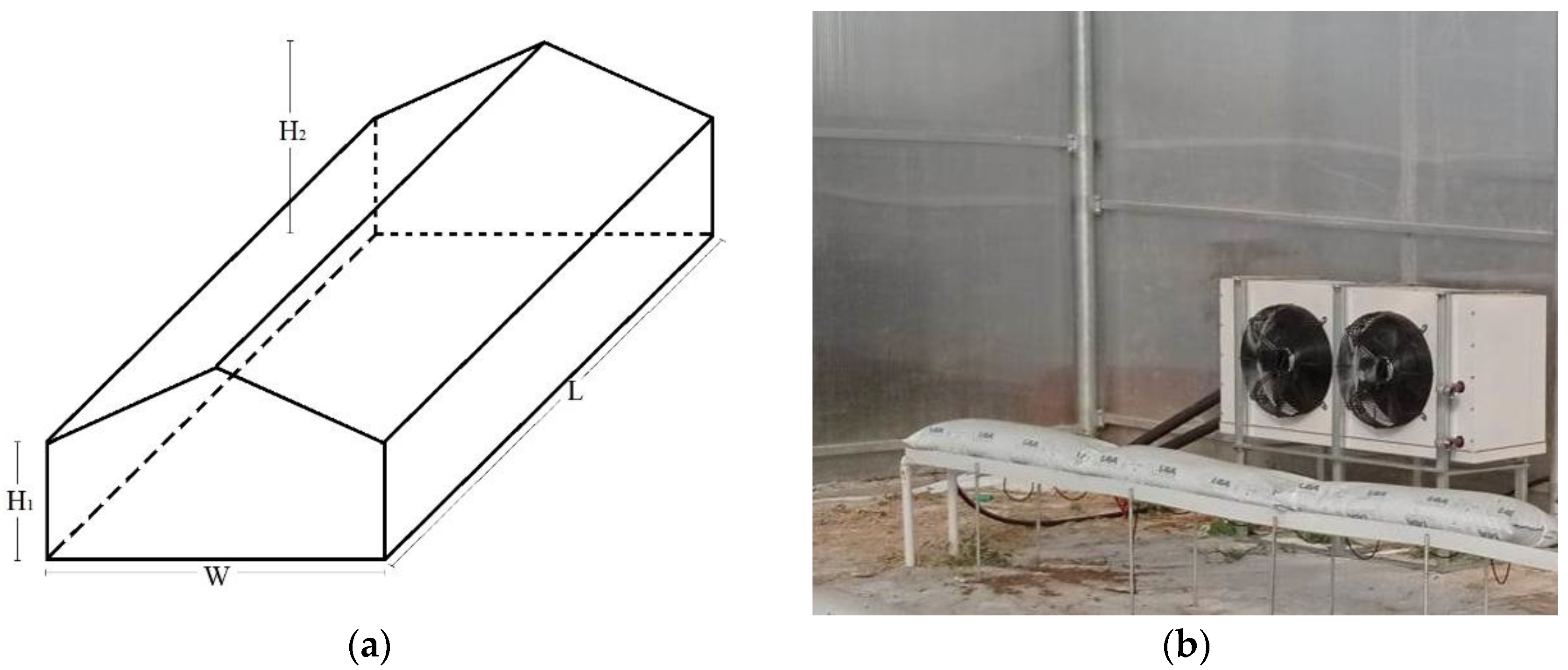
An experimental greenhouse facility located adjacent to the micro-CHP system served as the reference case for the simulations conducted in this study. The structure is an even-span greenhouse constructed with polycarbonate panels, featuring a length of 30 m (L), a width of 13.5 m (W), an eave height of 3.15 m (H₁), and a ridge height of 5.00 m (H₂), as illustrated in Figure 5a. The total surface area is 405 m², while its volume totals 1648.50 m³. Climate control within the greenhouse is achieved through forced ventilation via top windows oriented to the north and south, and space heating provided by fan coil-type air heaters (Figure 5b).

2.2. Thermal and Electrical Energy Requirements Modeling

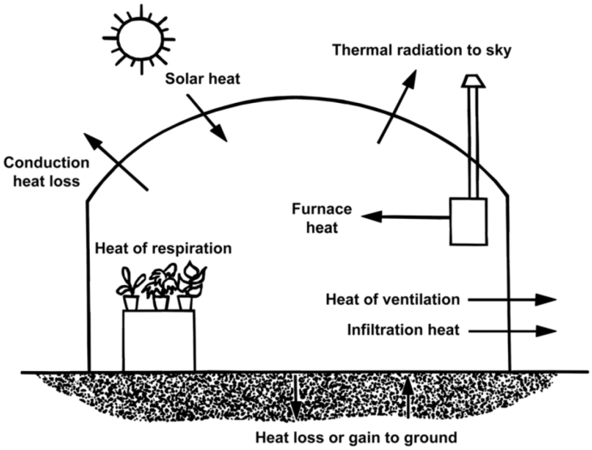
Calculating the greenhouse energy balance requires quantifying thermal interactions between exterior and interior environments, as well as moisture exchanges. Figure 6 illustrates the primary heat transfer mechanisms. Because these heat and mass fluxes vary continuously, dynamic calculations are needed to determine both thermal behavior and heating or cooling requirements.

Solar radiation reaching a greenhouse is partially absorbed or scattered by the atmosphere before striking the glazing. A portion is reflected, a small fraction absorbed by the glazing, and the remainder transmitted indoors. Heat exchange occurs via convection between the glazing and air, conduction through framing and insulation, and radiation between the glazing and internal surfaces. Transmitted solar energy is absorbed by plant canopies, soil, and internal structures, with retention aided by internal reflections and the greenhouse effect. Inside, plants exchange sensible heat with air and surfaces via convection and radiation, while evapotranspiration cools the leaf boundary through latent heat consumption. Similarly, the soil transfers heat by conduction, convection, and radiation, and loses latent heat through evaporation. Supplemental heating adds sensible heat to the air, while natural or forced ventilation removes both sensible and latent heat. Irrigation and fertigation influence soil moisture and humidity, affecting the greenhouse’s energy balance.

This work focuses on the economic feasibility of a CHP system, and for this reason, only the sensible heat loads are estimated. Accordingly, a simplified energy balance approach is adopted (as described in [45]). Outdoor temperature and solar radiation data from a typical meteorological year were used to calculate the heating load per unit of greenhouse surface area, as shown in Equation (1). The total required heating load (${\dot{Q}}_h$) is then calculated based on Equation (2).

$$H=\left[U\cdot {\displaystyle \frac{A_c}{A_f}}\cdot \left(T_{i,s}-T_o\right)\right]-\left(1-f\right)\cdot \tau \cdot \left(1-\rho \right)\cdot G_h$$

(1)

$${\dot{Q}}_h=H\cdot A_f$$

(2)

where

• H is the greenhouse heating load per sq. meter (W·m⁻²);
• U is the overall thermal transmittance (W·m⁻²·°C⁻¹);
• A_c is the cover and wall area (m²);
• A_f is floor area (m²);
• T_i,s is the indoor air temperature (setpoint) (°C);
• T_o is the outdoor air temperature (°C);
• f is the radiation to latent heat conversion factor inside the greenhouse (between 0.5 and 0.7);
• τ is the permeability to solar radiation factor (indicative value: 0.5);
• ρ is the reflectance coefficient of the interior (indicative value: 0.5);
• G_h is the solar radiation per sq. meter (W·m⁻²).

The parameters used in this simplified model are listed in

Table 3. The constant parameters in the model.

Coefficients	Symbol	Value	Unit
Overall thermal transmittance	U	4.20	W·m−2·°C−1
Cover area	Ac	783.13	m2
Floor area	Af	405.00	m2
Covers-to-Floor ratio	Ac/Af	1.93	[-]
Indoor air temperature (setpoint)	Ti,s	23.00	[°C]
Radiation to latent heat conversion factor inside the greenhouse	f	0.60	[-]
Permeability to solar radiation factor	τ	0.50	[-]
Reflectance coefficient of the interior	ρ	0.20	[-]

.

Electricity consumption has to be included in the calculations as well. This was performed by considering each electrically powered subsystem’s nominal power rating (e.g., lighting, irrigation pumps, shading system, dehumidifiers) and its daily operating hours throughout each cultivation stage. Section 3.2 elaborates on the electrical energy needs calculations for each growing stage.

2.3. Life Cycle Cost Analysis and Economic Indicators

Life Cycle Costing (LCC) is a method for estimating the total economic cost of a project by accounting for all resources consumed over its lifetime [46]. The cost categories and parameters required for the LCC calculation are [47,48] as follows:

• Initial capital cost (i.e., equipment purchase and installation);
• Operating cost (i.e., energy and fuel consumption);
• Maintenance and repair (OM&R) costs, including both annual and non-annual expenses;
• End-of-life cost (i.e., disposal or decommissioning).

In addition to these cost items, the analysis includes the equipment’s service life, the inflation rate, which is used to project future nominal costs, and the discount rate, which converts future expenditures to present value. The LCC is calculated using Equation (3), where C_INV denotes the initial investment costs, t the year in which a cost occurs, T is the system’s lifetime in years, C_tot is the cost, i.e., cash outflow, incurred in year t, and r is the discount rate [49].

$$LCC=C_{INV}+\sum _{t=0}^T{\displaystyle \frac{C_{out,tot}}{{\left(1+r\right)}^t}}$$

(3)

The total annual costs are the sum of the operating costs (C_O), maintenance (C_M), and end-of-life costs (C_E)—Equation (4). An inflation rate is applied to all cost parameters to project their future nominal values over the equipment’s lifetime.

$$C_{out,tot}=C_O\left(t\right)+C_M\left(t\right)+C_E\left(t\right)$$

(4)

Additionally, to provide a comprehensive assessment of economic viability, future costs are evaluated using three primary indicators, Net Present Value (NPV), Internal Rate of Return (IRR), and Discounted Payback Period (DPBP) [50], while applying a discount rate to convert future expenditures into present value.

In general, NPV is calculated by discounting all expected cash inflows (C_in) and outflows (C_out) over the project’s lifetime to their present values and then summing them. A positive NPV indicates that the present value of benefits exceeds that of costs, signaling a financially viable investment at the given discount rate. In the present study, NPV is applied to quantify the savings between the m-CHP and BAU scenarios (Equation (5), adapted from [51]), calculated by subtracting the sum of net cash flows (NCF) of the BAU scenario NCF_BAU from that of the m-CHP scenario NCF_m-CHP.

$$NPV=\sum _{t=0}^T{\displaystyle \frac{\left({NCF}_{m-CHP,t}-{NCF}_{BAU,t}\right)}{{\left(1+r\right)}^t}}$$

(5)

The Internal Rate of Return (IRR) is defined as the discount rate that makes the NPV of all project cash flows equal to zero, or, in other words, the IRR is the break-even discount rate where discounted inflows exactly offset discounted outflows. If the IRR exceeds the project’s required rate of return, the investment is considered acceptable; if it falls below, the project is not justified.

The Discounted Payback Period (DPBP) measures the length of time required for the discounted cumulative cash flows to recover the initial investment Equation (6). Unlike the simple payback period, DPBP thus accounts for the time value of money.

$$\sum _{t=0}^T{\displaystyle \frac{\left({NCF}_{m-CHP,t}-{NCF}_{BAU,t}\right)}{{\left(1+r\right)}^t}}\ge 0$$

(6)

Finally, the Levelized Cost of Energy (LCOE, Equation (7)) and Levelized Cost of Heat (LCOH, Equation (8)) are calculated. The equations are adapted from [52,53] and represent the lifetime cost per unit of energy output, defined as the system’s total LCC divided by its lifetime electrical energy generation (E_tot) and heat (Q_tot), respectively. Thus, LCOE is the cost per kilowatt-hour of electricity (EUR per kWh_el), and LCOH is the cost per kilowatt-hour of heat (EUR per kWh_th). The symbol a_el represents the cost allocation factor for the electricity generated from the micro-CHP unit, while a_he stands for the cost allocation factor for the heat generated by the cogeneration unit.

$$LCOE=a_{el} {\displaystyle \frac{LCC}{\sum _{t=0}^T{E}_{tot}}}$$

(7)

$$LCOH=a_{he}{\displaystyle \frac{LCC}{\sum _{t=0}^T{Q}_{CHP}}}$$

(8)

The values of a_el and a_he are determined in this work by applying the alternative generation method [52,53]. By following this approach, a_el and a_he are given by Equations (9) and (10), where n_el,ref (0.425) is the reference efficiency for electricity generation in Greece, and n_he,ref (0.85) is the efficiency of a typical natural gas boiler for heat generation [54].

$$a_{el}={\displaystyle \frac{E_{tot}/n_{el,ref}}{E_{tot}/n_{el,ref}+Q_{CHP}/n_{he,ref}}}$$

(9)

$$a_{he}={\displaystyle \frac{Q_{CHP}/n_{he,ref}}{E_{tot}/n_{el,ref}+Q_{CHP}/n_{he,ref}}}$$

(10)

2.4. Life Cycle Inventory

2.4.1. Initial Investment Costs

Initial investment costs are incurred only in the m-CHP scenario and cover one-time expenses at project inception. These include the ORC unit purchase (EUR 23,179.70), transportation of materials and installation of the biomass boiler, which replaces the conventional unit from the BAU scenario (EUR 1300.00), and a biomass storage tank for the boiler (EUR 500.00). The existing greenhouse heating distribution network requires no replacement or expansion; only minor modifications, which are already included in the retrofit and installation costs, are needed to connect the biomass boiler. The total initial investment of EUR 24,979.70 is summarized in

Table 4. Initial investment cost breakdown.

Cost Type	Cost (EUR)
ORC engine purchase costs	23,179.70
Transportation of equipment and materials	200.00
Boiler retrofitting and installation costs	1100.00
Biomass tank purchase costs	500.00
Total	24,979.70

, with a detailed breakdown of ORC engine component costs provided in

Table A3. Micro-CHP bill of materials and purchase costs.

Component	Model	Qty.	Unit Cost (EUR)	Cost (EUR)
Refrigerant pump	EDURAGGR LBM 406 A120 L/5.5 KW	1 pc.	6060.00	6060.00
Expander	Hanbell ER-230	1 pc.	5488.00	5488.00
Evaporator	SWEP V250ASHx120/1P	1 pc.	1550.00	1550.00
Condenser	SWEP B250ASHx96/1P	1 pc.	1150.00	1150.00
Ball valve	GMC 1.3/8″	1 pc.	46.80	46.80
Oil ball valve	GMC 5/8″	1 pc.	19.94	19.94
Oil solenoid	GMC 5/8″	1 pc.	46.80	46.80
Filter drier oil	GMC 5/8″	1 pc.	9.66	9.66
Oil receiver	Vertical 10Lt	1 pc.	130.00	130.00
Liquid receiver	Horizontal 50Lt	1 pc.	260.00	260.00
Filter drier	GMC 1.3/8″ with cartridge	1 pc.	47.97	47.97
PHE water connections	Victaulic 3″ silicone gasket	4 pcs.	11.93	47.74
Safety valve	GMC SV1/34	1 pc.	17.55	17.55
Suction line	Copper tube 2.5/8″	2.10 m	47.97	100.74
Discharge line	Copper tube 2.1/8″	1.32 m	37.44	49.42
Liquid line	Copper tube 1.3/8″	3.17 m	18.34	58.15
Oil line	Copper tube 5/8″	3.00 m	11.05	33.15
Pipe insulation	Armaflex 9 mm Φ54	1.32 m	1.30	1.72
Rotalolock valve	1.3/8″ (tube) in 1.3/4″ (flare)	2 pcs.	14.82	29.64
Frame	1.90 × 0.80 × 0.81 m	1 pc.	2000.00	2000.00
Pump connections	Flange JIS 1.1/2″	2 pcs.	7.44	14.87
Liquid indicator	GMC 1.3/8″	1 pc.	17.55	17.55
Electric panel with PLC	0.6 × 0.6 × 0.25 m	1 pc.	6000.00	6000.00
TOTAL				23,179.70

of Appendix A.

2.4.2. Operation and Maintenance Phase

During operation in both BAU and m-CHP scenarios, the unit costs for fuel (i.e., diesel and biomass) and electricity from the national grid are taken into account (

Table 5. Operation and maintenance costs under the BAU and m-CHP scenarios.

Operating Costs	Unit Cost
Diesel fuel (BAU)	EUR 1.12·L−1
Biomass fuel (BAU)	EUR 0.40·kg−1
Grid electricity (BAU and m-CHP)	EUR 0.1826·kWhel−1
Maintenance Costs	Cost (EUR)
BAU scenario	200.00
m-CHP scenario	270.00

), determining the ongoing expenses to meet the greenhouse’s energy demand. Finally, annual maintenance is estimated at EUR 200.00 for the BAU scenario, while for the m-CHP scenario, it amounts to EUR 270.00, including boiler cleaning (EUR 50.00), nozzle replacement (EUR 70.00), chimney cleaning (EUR 100.00), and working fluid refilling (EUR 50.00), summarized in Table 5 as well.

2.4.3. End-of-Life Stage

After 30 years of operation, the micro-CHP system is decommissioned, dismantled, and recycled. Modernization costs are prohibitively high, and when combined with its performance, continued operation is deemed uneconomical. The dismantling process itself incurs no significant costs. To enhance sustainability and generate profit, easily collectible and classifiable waste materials, specifically aluminum alloy, steel, plastic, and glass components, are recovered. Recovery rates for these materials are sourced from the literature [55], and their recycling values are based on average EU market prices shown in

Table 6. Materials recovered at the end-of-life of the micro-CHP system.

Material	Recovery Yields	Recovery Price (EUR·ton−1)
Plastic	90%	244.70
Aluminum	86%	2820.00
Steel	90%	500.00
Glass	9%	55.10

. At its end-of-life, the system yields 3000.00 kg of steel and 900.00 kg of aluminum solid waste. Recycling this equipment generates approximately EUR 4038.00 in revenue.

2.4.4. Economic Parameters

To estimate the annual cash flows and evaluate the economic performance of both scenarios over the system’s lifetime, several assumptions were made regarding key financial parameters. Fuel and energy prices are projected to rise annually, reflecting market forecasts, rather than remaining constant over the 30-year lifetime of the system. An inflation rate was set at 2.5%, in line with the Bank of Greece’s projection for the next years. Additionally, a 7% discount rate was applied to account for the time value of money, within the typical range of 6–8% for investments of this nature.

Although renewable energy projects in Greece are often eligible for EU and national subsidies, this study assumes project financing is provided either solely from own funds or through a combination of own funds and bank debt. In the debt-financed scenario, bank borrowing constitutes 70% of the initial investment. The interest rate for the loan was set at 5.5%, based on current interbank lending rates for a 15-year repayment period. The complete set of financial input data is summarized in

Table 7. Financial analysis input data.

Description	Value
Inflation	2.5%
Discount rate (r)	7%
Lifespan (years)	30
Loan-to-Cost Ratio (LTC)	0% or 70%
Loan interest rate	5.5%
Repayment term (years)	15

.

3. Results and Discussion

3.1. Greenhouse Heating Requirements and ORC Power Generation

For the simulations, two standard growing periods (GPs) within the year, i.e., 1st March to 30th June (GP1), and 1st September to 30th December (GP2), were considered. It should be noted that the greenhouse remains non-operational during July and August. Optimal indoor air temperature for cannabis growth typically ranges between 22 °C and 30 °C, while relative humidity is maintained between 65% and 70% [27]. Additionally, the ideal soil temperature ranges from 12 °C to 14 °C and should not fall below 6–8 °C. For the purposes of this study, the heating system setpoint temperature was fixed at 23 °C.

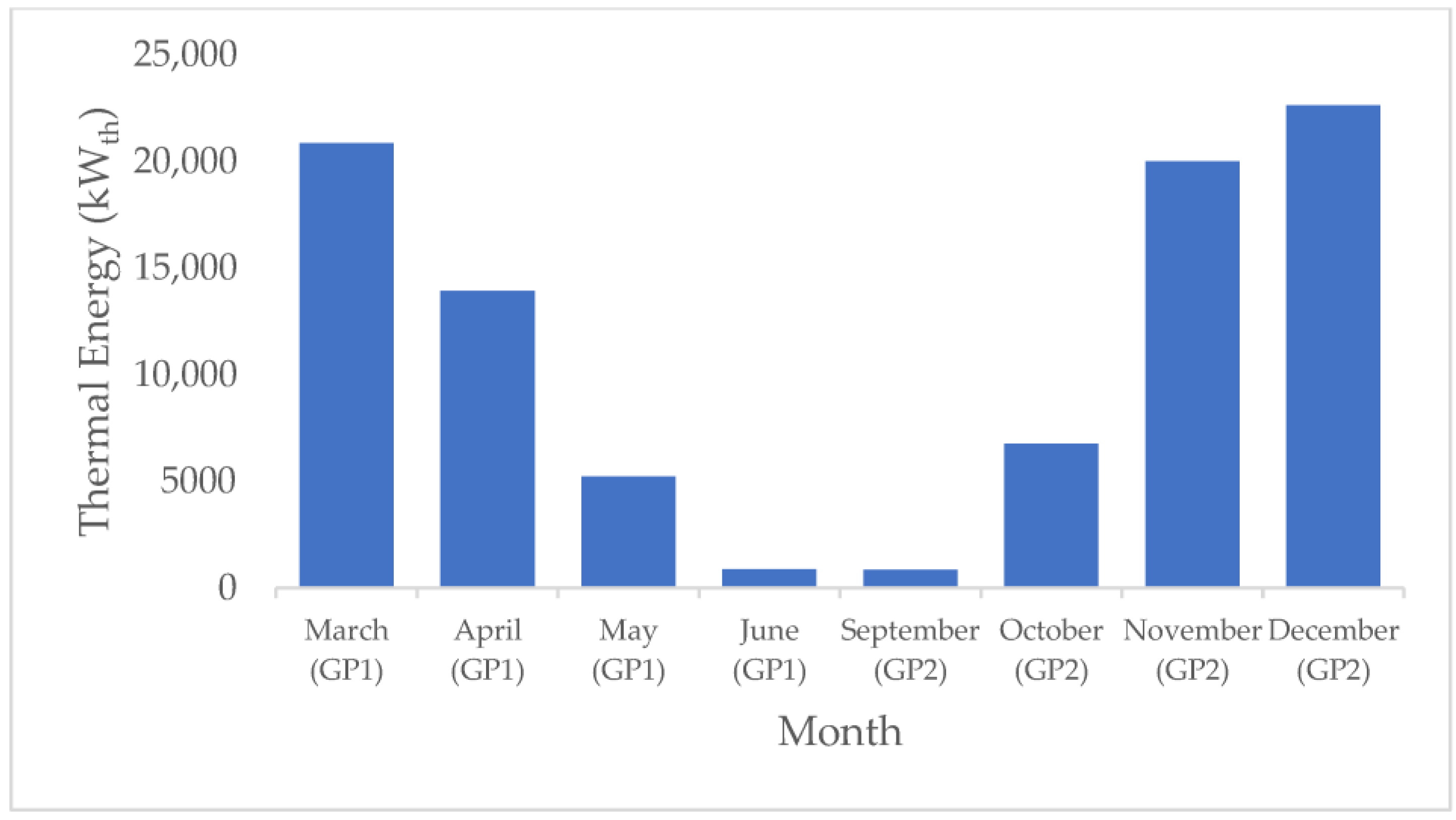
Based on Equation (2), the estimated thermal load profiles required for greenhouse heating throughout the two GPs over a full year are shown in Figure 7. Heating is required for a total of 3733 h annually, during which 91,065.20 kWh_th (224.58 kWhth·m⁻²) of thermal energy is supplied. The most energy-intensive months in GP1 are March (20,841.91 kWh_th) and April (13,914.90 kWh_th), while in GP2, the highest demand occurs in November (20,005.57 kWh_th) and December (22,628.34 kWh_th).

After estimating the total required heating load, the boiler’s fuel consumption was calculated (expressed as L·h⁻¹ for diesel and kg·h⁻¹ for biomass) using the assumed boiler efficiency, lower heating values (LHV), and densities listed in

Table 8. Fuel consumption-related assumptions of micro-CHP and BAU scenarios.

Coefficients	Value	Unit
Boiler Efficiency (diesel)	90%	[-]
Diesel LHV	11.62	kWh·kg−1
Diesel density	0.835	kg·L−1
Boiler Efficiency (biomass)	85%	[-]
Biomass LHV a	5.20	kWh·kg−1
Biomass pellet density	0.600	kg·L−1

^a Considering ENplus A1 class wood pellets, with a moisture content below 10% (wet basis, determined according to ISO 18134-1 [56] and compliant with ISO 17225-2 [57]).

.

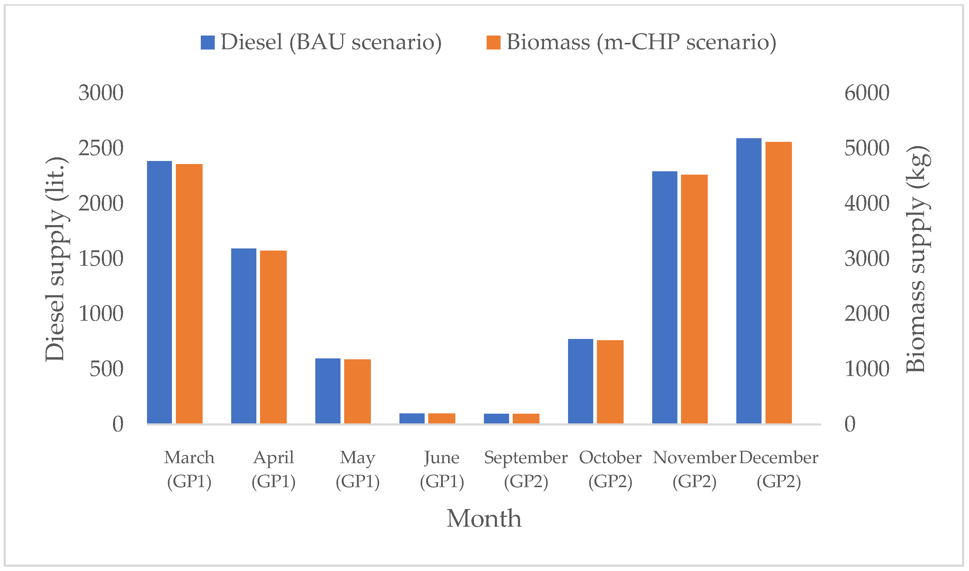
In the BAU scenario, the boiler requires an annual diesel supply of 10,428.39 L, whereas in the m-CHP scenario, the biomass boiler requires 20,602.99 kg to deliver the same thermal energy. The estimated monthly fuel supply profiles for each scenario are illustrated in Figure 8.

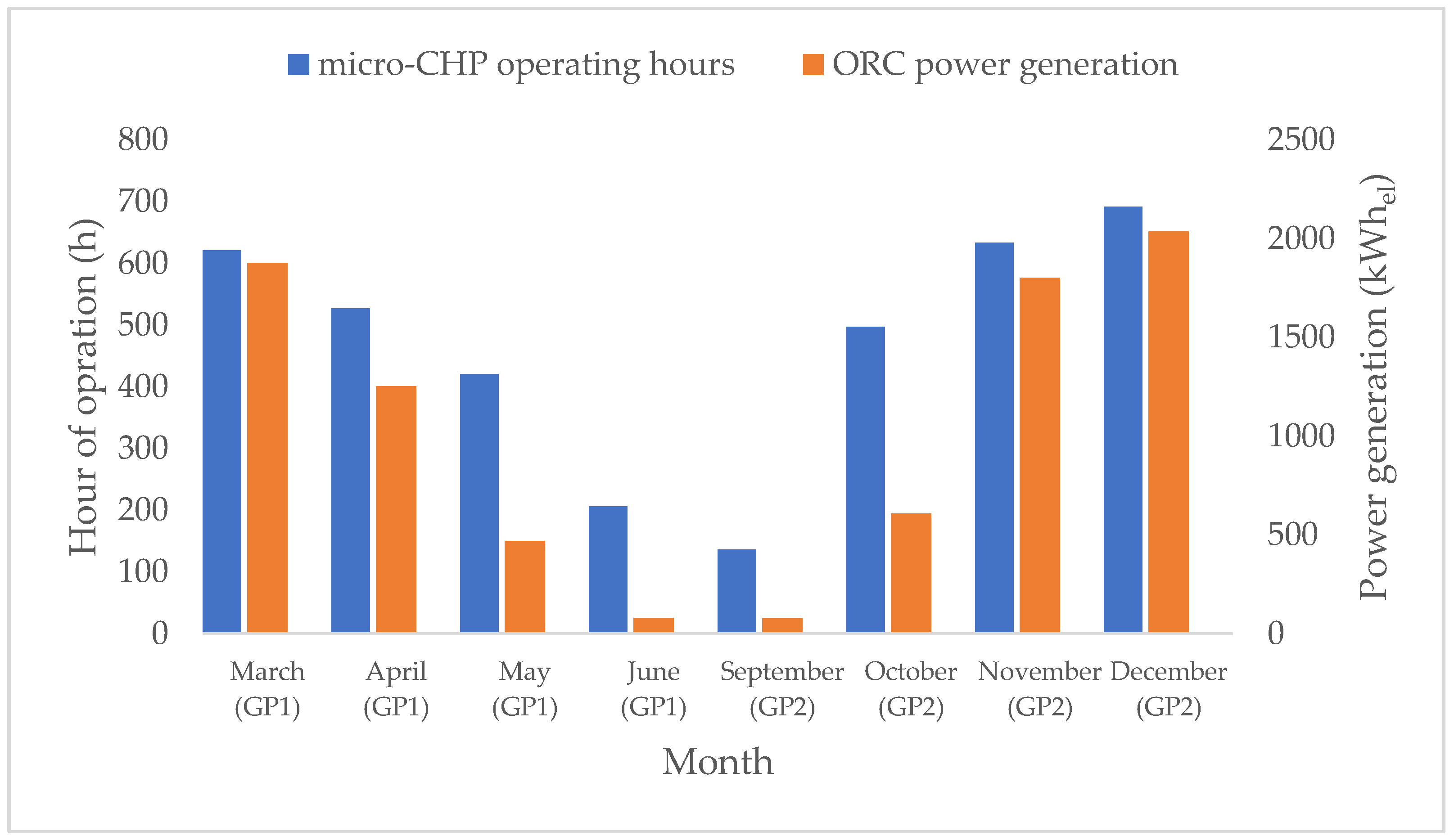
Based on the calculations performed, an 80 kW_th boiler is deemed sufficient for the specific application. To model the micro-CHP system’s hourly power generation and resulting electrical output, an average thermal efficiency of 9% was applied for a 7 kW_el ORC engine, considered reasonable based on available experimental data. Operating the proposed micro-CHP system with priority on covering the greenhouse heating is consistent with achieving high overall energy utilization while accepting the typical conversion efficiency at this scale. Specifically, lab-scale tests of a biomass-fired micro-ORC report net conversion efficiency up to 8.55% [58], whereas a hybrid solar–biomass micro-CHP achieved total energy efficiency up to 90.74% (exergy 15.05%) in a residential application [52]. The estimated monthly power generation output for the m-CHP scenario is illustrated in Figure 9, along with the corresponding monthly operating hours. On an annual basis, this corresponds to an estimated electrical energy production of 8195.87 kWh_el.

It should be noted that the system’s operating hours are influenced by the climatic conditions of the region where the greenhouse and the micro-CHP system are located. In colder regions, the system is expected to operate for more hours, as heating demand increases. Since power generation is directly linked to the operation of the heating system, this could potentially result in higher electricity output.

3.2. Greenhouse Electrical Energy Needs

The electrical energy requirements for the vegetative and flowering stages are presented in detail in

Table 9. Electrical energy needs for the vegetative stage from September to December (28 days).

System	Power (kW)	Operating Hours (h/day)	Daily Energy Consumption (kWhel)	Total Consumption (kWhel)
Lighting System	6.08	8.00	48.60	1360.80
Water pump	1.50	0.30	0.45	12.60
Shading system	5.00	2.00	10.00	280.00
Dehumidifiers	5.00	2.00	10.00	280.00
Total	-	-	-	1933.40

,

Table 10. Electrical energy needs for the flowering stage from September to December (56 days).

System	Power (kW)	Operating Hours (h/day)	Daily Energy Consumption (kWhel)	Total Consumption (kWhel)
Lighting System	6.08	4.00	24.30	1360.80
Water pump	1.50	0.30	0.45	25.20
Shading system	5.00	2.00	10.00	560.00
Dehumidifiers	5.00	2.00	10.00	560.00
Total	-	-	-	2506.00

,

Table 11. Electrical energy needs for the vegetative stage from March to June (28 days).

System	Power (kW)	Operating Hours (h/day)	Daily Energy Consumption (kWhel)	Total Consumption (kWhel)
Lighting System	6.08	4.00	24.30	680.40
Water pump	1.50	0.30	0.45	12.60
Shading system	5.00	2.00	10.00	280.00
Dehumidifiers	5.00	2.00	10.00	280.00
Total	-	-	-	1253.00

and

Table 12. Electrical energy needs for the flowering stage from March to June (56 days).

System	Power (kW)	Operating Hours (h/day)	Daily Energy Consumption (kWhel)	Total Consumption (kWhel)
Lighting System	6.075	2.00	12.15	680.40
Water pump	1.50	0.30	0.45	25.20
Shading system	5.00	2.00	10.00	560.00
Dehumidifiers	5.00	2.00	10.00	560.00
Total	-	-	-	1825.60

. During the September to December cultivation period, electricity consumption was 1933.40 kWh_el for the vegetative stage (Table 9) and 2506.00 kWh_el for the flowering stage (Table 10). In the March to June period, the vegetative stage required 1253.00 kWh_el (Table 11), while the flowering stage consumed 1825.60 kWh_el (Table 12).

Although the propagation stage involves significantly lower energy demands, it is not entirely negligible. To ensure a more accurate estimate of total annual energy use, an additional 5% has been added to account for the electrical energy consumed during propagation [26], resulting in a total annual electricity demand for operating environmental control systems and irrigation equipment estimated at 7893.90 kWh_el (19.36 kWh_el·m⁻²). The annual thermal energy and fuel consumption figures for the micro-CHP and BAU scenarios are summarized in

Table 13. Annual thermal energy and fuel consumption for the micro-CHP and BAU scenarios.

Parameter	Value	Unit
Thermal energy needs	91,065.20	kWhth
Boiler capacity	80.00	kWth
Diesel supply	10,428.39	L
Biomass supply	20,602.99	kg
Electrical energy needs	7893.90	kWhel
ORC unit capacity	7.00	kWel
ORC unit efficiency	9%	[-]
Power generation	8195.87	kWhel

. For a more detailed presentation of monthly electrical energy needs in each GP, refer to

Table A2. Monthly estimations of thermal energy needs, operating hours, fuel supply, and electrical energy generation for the micro-CHP and BAU scenarios.

Month [Growing Period]	Thermal Energy Demand (kWhth)	Micro-CHP Operating Hours (h)	Diesel Supply (L)	Biomass Supply (kg)	ORC Electrical Energy Generation (kWhel)
March [GP1]	20,841.91	621.00	2386.73	4715.37	1875.77
April [GP1]	13,914.90	527.00	1593.47	3148.17	1252.34
May [GP1]	5205.69	421.00	596.13	1177.76	468.51
June [GP1]	871.84	206.00	99.84	197.25	78.47
September [GP2]	848.89	136.00	97.21	192.06	76.40
October [GP2]	6748.07	497.00	772.76	1526.71	607.33
November [GP2]	20,005.57	633.00	2290.95	4526.15	1800.50
December [GP2]	22,628.34	692.00	2591.30	5119.53	2036.55
TOTAL	91,065.20	3733.00	10,428.39	20,602.99	8195.87

of Appendix A.

3.3. Operating Costs Under the BAU and m-CHP Scenarios

In the BAU scenario, meeting the greenhouse’s annual heating demand of 91,065.20 kWh_th requires diesel consumption that results in an annual fuel cost of EUR 11,679.80, based on an average diesel price of EUR 1.12·L⁻¹. Additionally, the total electricity consumption (7893.90 kWh_el), at an average price of EUR 0.1826·kWh_el⁻¹ [59], leads to an additional cost of EUR 1441.43. This brings the total annual operational expense to EUR 12,921.22. These figures are summarized in

Table 14. Annual operating costs under the BAU scenario.

Category	Quantity	Unit Cost	Total Cost (EUR)
Operating Costs
Diesel fuel consumption	10,428.39 L	EUR 1.12·L−1	11,679.80
Grid electricity consumption	7893.90 kWhel	EUR 0.1826·kWhel−1	1441.43
Total annual operating cost	—	—	12,921.22

.

Under the m-CHP scenario (see

Table 15. Annual operating costs and revenues under the m-CHP scenario.

Category	Quantity	Unit Cost (EUR)	Total Cost or Revenue (EUR)
Operating Costs
Biomass fuel consumption	20,602.99 kg	EUR 0.40·kg−1	8241.19
Grid electricity consumption	7893.90 kWhel	EUR 0.1826·kWhel−1	1441.43
Total annual operating cost	—	—	10,920.66
Generated Revenue
Electricity fed into the grid	8195.87 kWhel	EUR 0.1840·kWhel−1	—
Total annual generated revenue	—	—	1508.04

), the greenhouse requires 20,602.99 kg of biomass annually to meet its heating demand. At a retail price of EUR 0.40 per kg for biomass pellets, this results in a fuel cost of EUR 8241.19. Electricity consumption from the grid incurs the same cost as in the BAU scenario (EUR 1441.43), yielding a total annual expense of EUR 10,920.66. However, the ORC engine generates 8195.87 kWh_el of electricity annually, which, when sold to the local grid at a rate of EUR 0.1840 per kWh_el [59], applicable to non-household consumers, yields an additional gross revenue of EUR 1508.04 (Table 15).

3.4. Life Cycle Cost (LCC), Levelized Cost of Energy (LCOE), and Levelized Cost of Heat (LCOH)

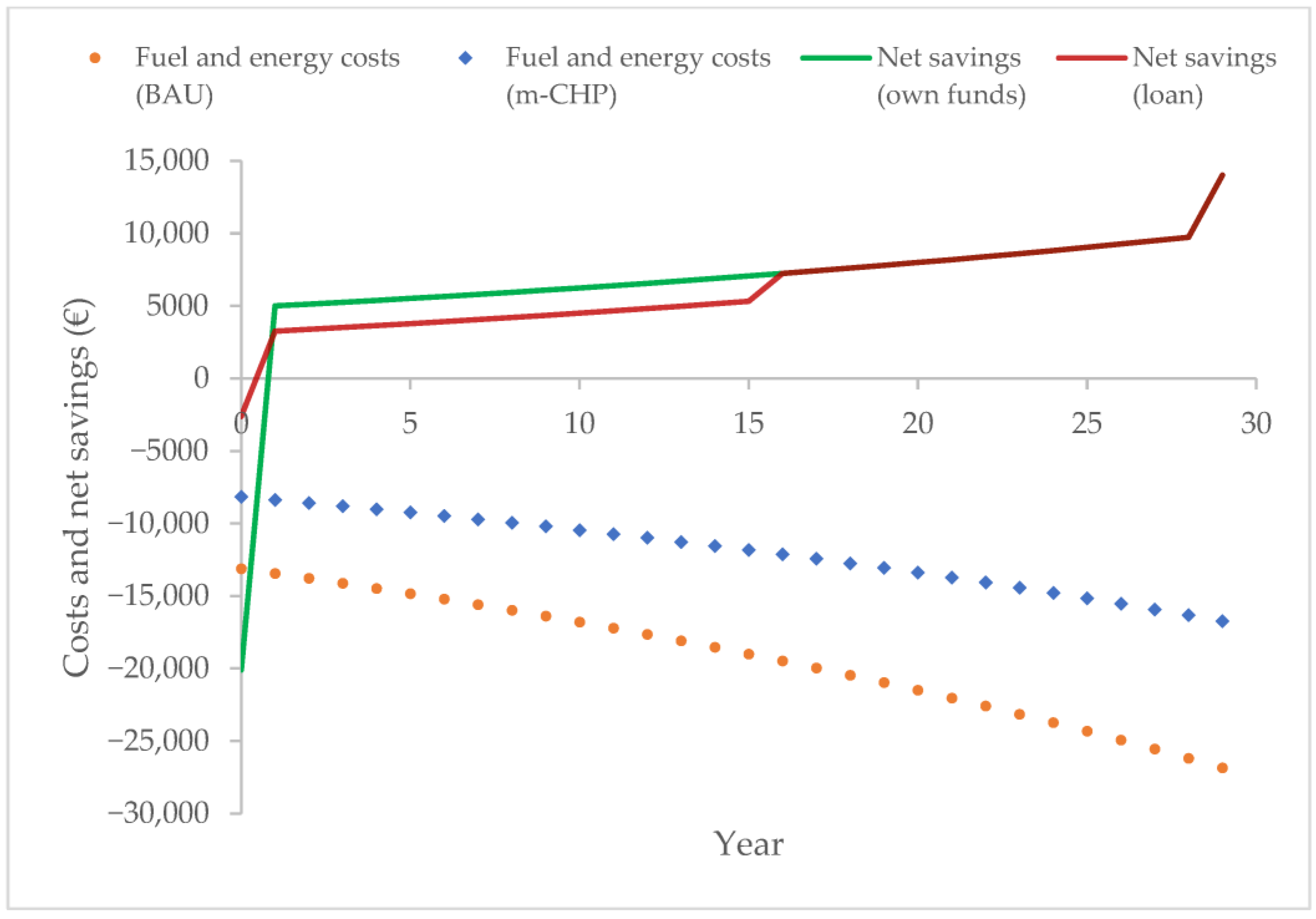
Using Equations (3) and (4), the LCC for the m-CHP scenario is calculated at EUR 196,421.33 over the system’s lifetime, representing a 14.4% reduction compared to the BAU scenario (EUR 229,468.46). Based on the undiscounted annual net cash flows, electricity revenues from the m-CHP system, and lower fuel costs yield cumulative savings of EUR 193,156.15. As shown in Figure 10, fuel and energy costs increase steadily on an annual basis due to the projected escalation of prices. In the BAU case, costs are largely driven by diesel purchases, whereas in the m-CHP case, the annual expenditure on fuel (biomass pellets) is ~29% lower. The two net savings curves reflect different financing structures: in the own-funds case, after the higher upfront investment in year 0, savings begin immediately and grow gradually, while in the loan-financed case, early-year savings are smaller due to debt service but converge after the loan is repaid (year 15). The steeper change in slope between year 0 and year 1 is driven by the difference in initial investment between the two cases, which affects annual net cash flows. Under 70% debt CAPEX financing (see Table 7), cumulative undiscounted savings decreased by EUR 8644.7, to EUR 184,511.45, reflecting the total principal and interest repayments.

The resulting LCOE and LCOH, EUR 0.122 per kWh_el and EUR 0.062 per kWh_th, respectively (

Table 16. Levelized Costs of Electricity (LCOE) and Heat (LCOH) in the micro-CHP scenario, alongside the key input parameters used for their calculation.

Parameter	Symbol	Value	Unit
Levelized Cost of Energy	LCOE	0.122	EUR·kWhel−1
Levelized Cost of Heat	LCOH	0.062	EUR·kWhth−1
Total electricity generated	Etot	245,876.04	kWhel
Total heat generated	QCHP	2,731,956.03	kWhth
Reference efficiency for electricity generation	nel,ref	0.425	-
Reference efficiency for heat generation	nhe,ref	0.850	-
Cost allocation factor for electricity	ael	0.150	-
Cost allocation factor for heat	ahe	0.850	-

), are highly competitive against current retail electricity and natural-gas prices for Greek non-household consumers (EUR 0.1578 per kWh_el and EUR 0.0401 per kWh_th), as well as against the EU averages (EUR 0.1515 per kWh_el and EUR 0.0535 per kWh_th) [60,61]. The cost allocation factors for electricity (a_el) and heat (a_he) are derived from Equations (9) and (10) based on the estimated total electricity (E_tot) and heat (Q_CHP) generated over the 30-year analysis period. If the loan on the initial investment is considered, both LCOE and LCOH are not significantly affected, showing only a reduction of 0.82% and 1.64%, respectively.

3.5. Net Present Value (NPV), Internal Rate of Return (IRR), and Discounted Payback Period (DPBP)

Under an all-equity financing structure, the m-CHP scenario delivers an NPV of EUR 59,591.88 and an un-levered IRR of 27.32%, indicating a highly attractive investment. When 70% of the capital expenditure is financed at 5.5% over 15 years (see

Table 17. Summary of key financial performance indicators for the m-CHP investment scenario compared to the BAU scenario.

Indicator		Scenario
	BAU	m-CHP (Own-Funds)	m-CHP (Loan)
LCC	EUR 229,468.46	EUR 196,421.33	EUR 194,801.82
NPV	-	EUR 59,591.88	EUR 61,211.39
DPBP	-	12.1 years	10.5 years

), the NPV increases by EUR 1619.51 to EUR 61,211.39. Thus, although servicing the debt reduces gross cash flows, it amplifies the project’s risk-adjusted returns. Finally, the DPBP is 12.1 years under the equity-financed scenario and 10.5 years under the debt-financed scenario, indicating a shorter capital repayment horizon under the leveraged structure. Table 15 presents a summary of the key financial performance indicators used to evaluate the m-CHP investment scenarios in comparison to the BAU case.

3.6. Sensitivity Analysis

While baseline projections assumed prices rising with inflation, a sensitivity analysis investigating plausible variations in key cost drivers (i.e., diesel, grid electricity, biomass costs, and RES electricity revenue) was also deemed necessary to provide additional insight into their effect on the financial performance of the innovative micro-CHP system.

Table 18. Sensitivity analysis scenarios and resulting key indicators.

Sensitivity Analysis Scenario			LCOE (EUR·kWhel−1)	LCOH (EUR·kWhhe−1)	LCC (EUR)	NPV (EUR)	DPBP (Years)
Baseline	Diesel cost (EUR·L−1)	1.12	0.122	0.062	196,421.33	59,591.88	12.13
	Grid electricity cost (EUR·kWh−1)	0.1826
	Biomass cost (EUR·kg−1)	0.40
	RES electricity revenue (EUR·kWh−1)	0.1840
Varying costs	Diesel cost (EUR·L−1)	0.90–1.15	0.122	0.062	196,421.33	20,071.70 to 127,854.00	>30 to 5.32
	Grid electricity cost (EUR·kWh−1)	0.15–0.25	0.119 to 0.128	0.060 to 0.64	191,988.43 to 205,586.29	59,591.88	12.13
	Biomass cost (EUR·kg−1)	0.30–0.50	0.100 to 0.144	0.050 to 0.072	160,931.09 to 231,911.58	95,082.12 to 24,101.63	7.41 to >30
	RES electricity revenue (EUR·kWh−1)	0.15–0.25	0.122	0.061	196,421.33	54,791.75 to 68,909.77	13.22 to 10.43
m-CHP favorable	Diesel cost (EUR·L−1)	1.232	0.112	0.056	179,736.83	96,505.05	7.06
	Grid electricity cost (EUR·kWh−1)	0.1643
	Biomass cost (EUR·kg−1)	0.36
	RES electricity revenue (EUR·kWh−1)	0.2024
BAU favorable	Diesel cost (EUR·L−1)	1.008	0.132	0.066	213,105.84	14,292.6	>>30
	Grid electricity cost (EUR·kWh−1)	0.2009
	Biomass cost (EUR·kg−1)	0.44
	RES electricity revenue (EUR·kWh−1)	0.1062

summarizes the sensitivity analysis scenarios and resulting key indicators (i.e., LCOE, LCOH, LCC, NPV, and DPBP). Using the m-CHP system (own-funds case) as the baseline, the main cost parameters were first varied individually within defined ranges to evaluate their impact on overall system performance. Subsequently, two scenarios were developed: one representing a condition more favorable to the m-CHP configuration and another favoring the BAU setup. In these, the most influential parameters were adjusted by approximately ±10% to reflect realistic shifts that would, respectively, benefit or challenge each configuration.

Although some indicators, such as LCOE, LCOH, and LCC, remained nearly constant in certain cases due to their definition and the system’s configuration, the sensitivity analysis highlights that fuel-related parameters exert a stronger influence on the project’s financial viability. Variations in diesel cost notably altered the DPBP from over 30 years to as low as 5.3 years, revealing how changes in fuel price can strongly affect investment attractiveness. Similarly, changes in biomass price significantly impacted both the levelized costs and the NPV, demonstrating that the system’s profitability is highly dependent on feedstock economics. In contrast, variations in grid electricity price and RES electricity revenue had comparatively modest effects on overall performance, as their relative contribution to total costs and revenues was smaller due to the energy exchange arrangement with the grid.

In the m-CHP favorable scenario, the combination of a higher diesel price, slightly lower grid cost, lower biomass price, and higher RES electricity revenue represents conditions that favor the micro-CHP system. Under these assumptions, both the LCOE and LCOH decrease, while the NPV rises substantially and the DPBP shortens to just over 7 years. This demonstrates a strong improvement in system profitability and cost-effectiveness, confirming that when RES and electricity revenues align favorably, the micro-CHP configuration becomes highly competitive and financially robust. On the other hand, the scenario representing conditions more advantageous to the conventional system (BAU approach) results in poorer economic performance. This case yields higher LCOE and LCOH values, a higher LCC, a substantially lower NPV, and an exceedingly long payback period exceeding 30 years. These results clearly indicate that, under these assumptions, the conventional configuration is less economically attractive compared to the m-CHP alternative.

3.7. Environmental Aspects

Along with the generally positive assessment of the economic feasibility of the innovative biomass-fired micro-CHP system for medicinal cannabis cultivation, the environmental performance of the greenhouse facility also shows a significant improvement. The transition from diesel to sustainably sourced biomass substantially reduces GHG emissions. As presented in

Table 19. Fuel characteristics, emission factors, and calculated greenhouse gas emissions for diesel and wood pellet combustion.

Parameter	Unit	Diesel Fuel	Wood Pellet Biomass
Fuel consumption	kg	8707.71	20,602.99
Energy content	kWh·kg−1	11.62	5.2
	TJ·kg−1	4.18 × 10−5	1.87 × 10−5
Total energy used	TJ	0.36	0.39
CO2 GWP a	kg·TJ−1	74,100.00	112,000.00
NH4 GWP a	kg·TJ−1	3.00	30.00
N2O GWP a	kg·TJ−1	0.60	4.00
Emitted CO2	kg	26,972.40	0.00 b
Emitted CH4	kg	1.09	11.58
Emitted N2O	kg	0.22	1.54
CO2 × GWP	kg CO2-equivalent	26,972.40	0
CH4 × GWP c	kg CO2-equivalent	30.58	324.24
N2O × GWP c	kg CO2-equivalent	57.88	409.16
Total GHG emissions	kg CO2-equivalent	27,060.85	733.40

^a IPCC 2006 defaults for stationary combustion on a net calorific basis [62]. ^b The biogenic CO₂ emissions from pellet combustion (≈43.2 tCO₂) are not included in the net fossil totals, consistent with IPCC reporting practice that considers CO₂ from sustainably sourced biomass as biogenic and carbon-neutral, while excluding upstream supply-chain emissions from the combustion inventory. ^c GWP values are from the IPCC AR5 (CH₄ = 28, N₂O = 265).

, replacing diesel with ENplus A1 wood pellets effectively eliminates net fossil CO₂ emissions (26.97 tCO₂), resulting in an estimated reduction of approximately 26.33 tCO₂-eq (97.3%) in reported GHG emissions, assuming the biomass is sustainably sourced.

Additional CO₂ emission reductions can be attributed to RES electricity generation, which is treated as avoided grid electricity production. Specifically, assuming an average national grid carbon intensity of 269 gCO₂·kWh⁻¹ for 2024 [63], the avoided generation of 301.97 kWh_el (Table 12) corresponds to approximately 81.23 kg of avoided CO₂ emission, resulting in a total of 27.01 tCO₂.

3.8. Comparative Analysis of Alternative Energy Technologies for Greenhouse Applications

While not strictly comparable, the studied biomass-fired micro-CHP system appears to occupy a middle ground in techno-economic performance relative to both innovative and conventional technologies used in greenhouse settings. Although it offers a slower payback than biomass systems providing only heating, the on-site electricity generation could offset most purchased electricity and reduce exposure to grid price fluctuations. Compared with heat pump (HP) options, it is more resilient in contexts where power tariffs are high or drilling is costly. Unlike natural gas (NG) CHP, it avoids exposure to fossil fuel price volatility and potential carbon-pricing schemes, while remaining financially attractive in the modeled context.

More specifically, biomass heating-only options that use flue gases for soil or air heating in greenhouses in China have demonstrated payback periods (DPBPs) of less than three years when biomass is inexpensive [64]. Similar findings were reported for a 1000 m² greenhouse in Crete, Greece, where a solid biomass boiler achieved a payback of 2.95 years [65]. An earlier Canadian study [66] also showed that installing a biomass boiler to meet 40% of annual heating demand was more economical than using a natural gas boiler to supply the full load. However, these systems do not produce electricity.

The economics of gas-engine CHP systems are primarily governed by the spark ratio (i.e., the ratio of electricity price to natural gas price) and the potential to monetize CO₂ for enrichment. A pan-European analysis found that when the spark ratio exceeds 4, negative net heat costs can be achieved (i.e., the combined electricity and CO₂ value exceeds the fuel cost) [67]. Depending on operational strategy, daily dynamic optimization in Dutch greenhouses equipped with CHP, boilers, HPs, thermal buffers, and aquifer storage reduced energy costs by up to 29% compared to baseline grower dispatch [68].

For air-source heat pumps (ASHPs), measured Seasonal Coefficients of Performance (SCOPs) between 1.5 and 3.0 can yield relatively short payback periods (around 5.5 years). Ground-source heat pumps (GSHPs), while offering lower operating costs, typically have paybacks of around 18 years unless cheap electricity or favorable geothermal conditions are available [69,70]. Hybrid systems combining photovoltaic–thermal (PVT) panels with GSHPs have achieved COPs of 3.38 and 78% heating cost savings relative to kerosene, although their electricity generation offsets only 36.72% of HP electricity consumption, and performance strongly depends on hydrogeological conditions and local fuel benchmarks [71].

Finally, a recent feasibility study on greenhouse–fuel cell convergence systems reported benefit–cost ratios of 0.62–0.65 for farmer-led models and 1.19–1.86 for utility-led models [72]. In that study, the fuel-cell CHP was benchmarked against geothermal HP greenhouse systems, highlighting capital expenditure and policy support as decisive factors.

Beyond the reference case, biomass-ORC micro-CHP could be most advantageous in colder climates or in places with long, steady heating seasons, where higher run hours would increase annual electricity yield and shorten the payback period. In warmer climates, PV/PVT-assisted, high-SCOP heat-pump architectures may outperform, particularly where electricity tariffs are low. The micro-CHP configuration could also suit grid-constrained or outage-prone locations, utilizing on-site generation, electricity storage, and modest thermal buffering. A detailed, case-specific techno-economic assessment should be conducted beforehand to assess performance, as investment costs can be substantial.

If biomass-ORC micro-CHP were widely adopted, potential benefits could arise at multiple levels. By substituting biomass, substantial fossil CO₂ abatement could be achieved. Moreover, where biomass residues are abundant, local bioenergy value chains and regional circularity could be strengthened. However, using residual biomass rather than certified pellets introduces quality risks (e.g., lower energy content, ash) and necessitates the use of emission-certified boilers. This may also increase O&M needs (ash handling, fouling control, periodic cleaning) and entail local air-quality compliance obligations. Moreover, renewable-electricity production, paired with storage or a favorable interconnection/metering arrangement, could considerably reduce exposure to electricity-price volatility and improve the greenhouse sector’s resilience.

4. Conclusions

The techno-economic assessment of a biomass-fired micro-CHP system integrated with an ORC unit for a medicinal cannabis greenhouse demonstrates clear financial advantages over the conventional diesel-boiler configuration. For the greenhouse studied, the estimated annual energy intensities are consistent with the recent literature on protected cannabis cultivation once differences in operational practices and local climate are considered, with an estimated annual heating demand of 224.58 kWh_th·m⁻² (91,065.20 kWh_th), and electricity use of 19.36 kWh_el·m⁻² (7839.90 kWh_el). Over a thirty-year lifetime, the micro-CHP scenario (80 kW_th boiler retrofitted for biomass and a 7 kW_el ORC engine) reduces the life-cycle cost from EUR 229,468.46 to EUR 196,421.33 when fully equity-financed, and to EUR 194,801.82 with 70% debt financing, representing savings up to approximately 14.4%. These savings translate into a positive net present value of EUR 59,591.88 (own-funds) and EUR 61,211.39 (leveraged), while the discounted payback period shortens from 12.1 years to 10.5 years under the debt-financed case. The internal rate of return of 27.32% under all-equity financing further confirms the project’s attractiveness.

In addition to cost reductions, the micro-CHP configuration yields highly competitive levelized costs of electricity (EUR 0.122·kWh_el) and heat (EUR 0.062·kWh_th). These figures undercut typical retail electricity and natural-gas prices in Greece and compare favorably to EU averages. Though the on-site generation of 8195.87 kWh_el per year exceeds just by 4% the greenhouse’s electricity requirements, it generates additional revenues for the producer. From an environmental standpoint, switching from diesel to biomass, ideally sourced from cannabis residue or local agricultural waste, reduces reliance on fossil fuels and lowers CO₂ emissions (27.01 tCO₂ reduction) and total GHG emissions. When combined with other best practices such as LED lighting, off-peak scheduling, and CO₂ enrichment via waste-heat recovery, the micro-CHP system advances the greenhouse toward a circular and sustainable operation.

The study evaluates an innovative micro-CHP system in a high-value greenhouse operation, providing insights into techno-economic performance, system optimization, and environmental impact. Socially, it highlights tangible benefits in operational cost reduction, energy autonomy, emission mitigation, and circular resource utilization, contributing to more sustainable, resilient, and economically viable practices in the agricultural sector. Biomass-ORC micro-CHP systems are well-suited to colder or grid-constrained sites with long heating seasons and reliable biomass supply. At scale, they cut GHG emissions and moderate power-price volatility, but require attention to feedstock quality, O&M practices, air-quality compliance, and storage/safety requirements. Future research should focus on dynamic control strategies and energy storage, both electrical and thermal, options that optimize ORC operation under real-time thermal loads, undertake detailed life-cycle carbon-footprint analysis, and evaluate at the techno-economic level the combined heat, power, and CO₂ utilization schemes in cannabis greenhouses.

References

1. Saragoça, A.; Silva, A.C.; Varanda, C.M.R.; Materatski, P.; Ortega, A.; Cordeiro, A.I.; Telo da Gama, J. Current Context of Cannabis sativa Cultivation and Parameters Influencing Its Development. Agriculture 2025, 15, 1635. [Google Scholar] [CrossRef]
2. Thetsane, R.M. Envisaging Challenges for the Emerging Medicinal Cannabis Sector in Lesotho. J. Cannabis Res. 2024, 6, 23. [Google Scholar] [CrossRef]
3. Dillis, C.; Polson, M.; Bodwitch, H.; Carah, J.; Power, M.E.; Sayre, N.F. Industrializing Cannabis? Socio-Ecological Implications of Legalization and Regulation in California. In The Routledge Handbook of Post-Prohibition Cannabis Research; Corva, D., Meisel, J.S., Eds.; Routledge: London, UK, 2021; pp. 221–230. [Google Scholar]
4. Chatzigianni, C.; Roussis, I.; Papadas, C.T.; Karidogianni, S.; Kouneli, V.; Kakabouki, I.; Folina, A.; Papastylianou, P.; Bilalis, D. Estimated Cost of Production for Medical Cannabis (Cannabis sativa L.) in Greece. Bull. UASVM Hortic. 2020, 77, 1843–5394. [Google Scholar] [CrossRef]
5. Hellenic Republic. Law No. 4523—Gov. Gazette A’ 41/07.03.2018; Government Gazette, National Printing Office: Athens, Greece, 2018. (In Greek)
6. Folina, A.; Roussis, I.; Kouneli, V.; Kakabouki, I.; Karidogianni, S.; Bilalis, D. Opportunities for cultivation of medical cannabis (Cannabis sativa L.) in Greece. Sci. Pap. Ser. A. Agron. 2019, 62, 293–300. [Google Scholar]
7. Collado, C.E.; Hwang, S.J.; Hernández, R. Supplemental Greenhouse Lighting Increased the Water Use Efficiency, Crop Growth, and Cutting Production in Cannabis sativa. Front. Plant Sci. 2024, 15, 1371702. [Google Scholar] [CrossRef]
8. Dohlman, E.; Maguire, K.; Davis, W.V.; Husby, M.; Bovay, J.; Weber, C.; Lee, Y. Trends, Insights, and Future Prospects for Production in Controlled Environment Agriculture and Agrivoltaics Systems; Economic Information Bulletin, No. 264; U.S. Department of Agriculture, Economic Research Service: Washington, DC, USA, 2024. Available online: https://www.ers.usda.gov/sites/default/files/_laserfiche/publications/108221/EIB-264.pdf (accessed on 4 November 2025).
9. Azzaretti, C.; Carleton, B. CEA Energy & Water Benchmarking Report: Establishing Preliminary Benchmarks for Controlled Environment Agriculture (CEA) Operations; Resource Innovation Institute: Portland, OR, USA, 2023; Available online: https://resourceinnovation.org/wp-content/uploads/2023/08/RII-Benchmarking_2023.pdf (accessed on 4 November 2025).
10. Bafort, F.; Libault, A.; Maron, E.; Kohnen, S.; Ancion, N.; Jijakli, M.H. Operational Costs and Analysis of Agronomic Characteristics on Cannabidiol and Cannabigerol Hemp (Cannabis sativa L.) in Hydroponic Soilless Greenhouse and Field Cultivation. Horticulturae 2024, 10, 1271. [Google Scholar] [CrossRef]
11. Charles, A.P.R.; Gu, Z.; Archer, R.; Auwarter, C.; Hatterman-Valenti, H.; Rao, J.; Chen, B. Effect of High-Tunnel and Open-Field Production on the Yield, Cannabinoids, and Volatile Profiles in Industrial Hemp (Cannabis sativa L.) Inflorescence. J. Agric. Food Chem. 2024, 72, 12975–12987. [Google Scholar] [CrossRef] [PubMed]
12. Syed, A.; Hachem-Vermette, C. Climate Change Resilient Urban Prototypes—A Canadian Perspective on Net Zero Energy Design for Retail Amenities. Energy Eng. 2019, 116, 7–25. [Google Scholar] [CrossRef]
13. Marcelis, L.F.M.; Costa, J.M.; Heuvelink, E. Achieving Sustainable Greenhouse Production: Present Status, Recent Advances and Future Developments. In Achieving Sustainable Greenhouse Production; Marcelis, L.F.M., Heuvelink, E., Eds.; Burleigh Dodds Science Publishing: Cambridge, UK, 2019; pp. 1–14. [Google Scholar]
14. Mills, E. Comment on “Cannabis and the Environment: What Science Tells Us and What We Still Need to Know”. Environ. Sci. Technol. Lett. 2021, 8, 483–485. [Google Scholar] [CrossRef]
15. Independent Electricity System Operator (IESO). Energy Management Best Practices for Cannabis Greenhouses and Warehouses; IESO: Toronto, ON, Canada, 2021. [Google Scholar]
16. Mills, E. The Emergence of Indoor Agriculture as a Driver of Global Energy Demand. NPJ Sustain. Agric. 2025, 3, 52. [Google Scholar] [CrossRef]
17. Kamminga, J.; Me, A. The Blind Men and the Elephant: Measuring the Environmental Impact of Cannabis. J. Illicit Econ. Dev. 2025, 7, 1–13. [Google Scholar] [CrossRef]
18. Massachusetts Department of Energy Resources. Cannabis Energy Overview and Recommendations; Massachusetts Cannabis Control Commission: Boston, MA, USA, 2018. [Google Scholar]
19. Mills, E. The Carbon Footprint of Indoor Cannabis Production. Energy Policy 2012, 46, 58–67. [Google Scholar] [CrossRef]
20. Cola, G.; Mariani, L.; Toscano, S.; Romano, D.; Ferrante, A. Comparison of Greenhouse Energy Requirements for Rose Cultivation in Europe and North Africa. Agronomy 2020, 10, 422. [Google Scholar] [CrossRef]
21. Sanford, S. Reducing Greenhouse Energy Consumption—An Overview; University of Wisconsin, Extension Service Report; University of Wisconsin: Madison, WI, USA, 2011. [Google Scholar]
22. Summers, H.M.; Sproul, E.; Quinn, J.C. The Greenhouse Gas Emissions of Indoor Cannabis Production in the United States. Nat. Sustain. 2021, 4, 644–650. [Google Scholar] [CrossRef]
23. Mills, E. Energy-Intensive Indoor Cultivation Drives the Cannabis Industry’s Expanding Carbon Footprint. One Earth 2025, 8, 101179. [Google Scholar] [CrossRef]
24. Moreno, R.M. Dimensionamento e Análise Energética de uma Estufa de Cannabis Medicinal. Master’s Thesis, Instituto Superior Técnico, Universidade de Lisboa, Lisbon, Portugal, 2020. (In Portuguese). [Google Scholar]
25. van Gruisen, D.; van Noort, F. Towards Energy-Neutral Cannabis Cultivation: Exploring Energy Efficiency and Carbon Footprint Mitigation Strategies—A Desk Study on Regulated Medical Cannabis Production; Kas als Energiebron/Wageningen University & Research: Wageningen, The Netherlands, 2024. [Google Scholar]
26. New Frontier Data. The 2018 Cannabis Energy Report; New Frontier Data: Washington, DC, USA, 2018. [Google Scholar]
27. Wells, M.J. Expert Opinion: How Humidity Works. Cannabis Business Times. 2017. Available online: https://www.cannabisbusinesstimes.com/home/article/15703674/moisture-matters (accessed on 4 November 2025).
28. National Cannabis Industry Association. Environmental Sustainability in the Cannabis Industry: Impacts, Best Management Practices, and Policy Considerations; NCIA: Washington, DC, USA, 2020. [Google Scholar]
29. Canova, A.; Chicco, G.; Genon, G.; Mancarella, P. Emission Characterization and Evaluation of Natural Gas-Fueled Cogeneration Microturbines and Internal Combustion Engines. Energy Convers. Manag. 2008, 49, 2900–2909. [Google Scholar] [CrossRef]
30. Seiler, J.C.; Pavlak, G.; Freihaut, J.D. Energy Dispatch Optimization at Controlled Environment Agriculture Sites with CHP: How Energy Utilization, Storage, and Market Exports Impact Operational Costs. Energy Convers. Manag. 2025, 332, 119743. [Google Scholar] [CrossRef]
31. Vermeulen, P.C.M.; van der Lans, C.J.M. Combined heat and power (CHP) as a possible method for reduction of the CO2 footprint of organic greenhouse horticulture. In Proceedings of the I International Conference on Organic Greenhouse Horticulture, Bleiswijk, The Netherlands, 11–14 October 2010; Dorais, M., Bishop, S.D., Eds.; ISHS: Leuven, Belgium, 2011; Volume 915, pp. 61–68. [Google Scholar]
32. Compernolle, T.; Witters, N.; Van Passel, S.; Thewys, T. Analyzing a Self-Managed CHP System for Greenhouse Cultivation as a Profitable Way to Reduce CO2-Emissions. Energy 2011, 36, 1940–1947. [Google Scholar] [CrossRef]
33. Abbass, A. Hybrid Solar CHP Microgrid Optimization: Python Code Framework Using Real Equipment Data. Adv. Eng. Lett. 2025, 4, 164–174. [Google Scholar] [CrossRef]
34. Arsalis, A. A Comprehensive Review of Fuel Cell-Based Micro–Combined-Heat-and-Power Systems. Renew. Sustain. Energy Rev. 2019, 105, 391–414. [Google Scholar] [CrossRef]
35. Cardoso, D.; Nunes, D.; Faria, J.; Fael, P.; Gaspar, P.D. Intelligent Micro-Cogeneration Systems for Residential Grids: A Sustainable Solution for Efficient Energy Management. Energies 2023, 16, 5215. [Google Scholar] [CrossRef]
36. Kallio, S.; Siroux, M. Hybrid Renewable Energy Systems Based on Micro-Cogeneration. Energy Rep. 2022, 8 (Suppl. S1), 762–769. [Google Scholar] [CrossRef]
37. Hammond, G.P.; Titley, A.A. Small-Scale Combined Heat and Power Systems: The Prospects for a Distributed Micro-Generator in the ‘Net-Zero’ Transition within the UK. Energies 2022, 15, 6049. [Google Scholar] [CrossRef]
38. Gul, E.; Baldinelli, G.; Bartocci, P. Energy Transition: Renewable Energy-Based Combined Heat and Power Optimization Model for Distributed Communities. Energies 2022, 15, 6740. [Google Scholar] [CrossRef]
39. Dobre, C.; Costin, M.; Constantin, M. A Review of Available Solutions for Implementation of Small–Medium Combined Heat and Power (CHP) Systems. Inventions 2024, 9, 82. [Google Scholar] [CrossRef]
40. Bellos, E. A Review of Organic Rankine Cycles with Partial Evaporation and Dual-Phase Expansion. Sustain. Energy Technol. Assess. 2024, 72, 104059. [Google Scholar] [CrossRef]
41. Lecompte, S.; Huisseune, H.; Van Den Broek, M.; Vanslambrouck, B.; De Paepe, M. Review of Organic Rankine Cycle (ORC) Architectures for Waste Heat Recovery. Renew. Sustain. Energy Rev. 2015, 47, 448–461. [Google Scholar] [CrossRef]
42. Karellas, S.; Leontaritis, A.D.; Panousis, G.; Bellos, E.; Kakaras, E. Energetic and Exergetic Analysis of Waste Heat Recovery Systems in the Cement Industry. Energy 2013, 58, 147–156. [Google Scholar] [CrossRef]
43. ORC World Map. Available online: https://orc-world-map.org/ (accessed on 4 November 2025).
44. Worley, J. Greenhouses: Heating, Cooling and Ventilation; Bulletin 792; University of Georgia, UGA Extension: Athens, GA, USA, 2014. [Google Scholar]
45. Cecilia, S.; Heuvelink, E.; Ooster, B.V. Greenhouse Horticulture: Technology for Optimal Crop Production, 2nd ed.; Brill|Wageningen Academic: Wageningen, The Netherlands, 2024; ISBN 9789004697041. [Google Scholar]
46. Bagg, M. Save Cash and Energy Costs via an LCC Model. World Pumps 2013, 12, 18–21. [Google Scholar] [CrossRef]
47. Cheng Hin, J.N.; Zmeureanu, R. Optimization of a Residential Solar Combisystem for Minimum Life Cycle Cost, Energy Use and Exergy Destroyed. Sol. Energy 2014, 100, 102–113. [Google Scholar] [CrossRef]
48. Gkoloni, N.; Golonis, C.; Kostopoulos, V. Integration of LCA and LCC for Decision Making in Biocomposite Production. Proc. IOP Conf. Ser. Earth Environ. Sci. 2022, 1123, 012071. [Google Scholar] [CrossRef]
49. Chaurasiya, P.K.; Azad, A.K.; Warudkar, V.; Ahmed, S. Advancement in Remote Sensing of Wind Energy. In Advances in Clean Energy Technologies; Azad, A.K., Ed.; Academic Press: Cambridge, MA, USA, 2021; pp. 207–233. [Google Scholar]
50. Spertino, F.; Di Leo, P.; Cocina, V. Economic Analysis of Investment in the Rooftop Photovoltaic Systems: A Long-Term Research in the Two Main Markets. Renew. Sustain. Energy Rev. 2013, 28, 531–540. [Google Scholar] [CrossRef]
51. Kumar, L.; Mamun, M.A.A.; Hasanuzzaman, M. Energy Economics. In Energy for Sustainable Development; Hasanuzzaman, M., Abd Rahim, N., Eds.; Academic Press: Cambridge, MA, USA, 2020; pp. 167–178. [Google Scholar]
52. Skiadopoulos, A.; Kosmadakis, G.; van Heule, X.; Lecompte, S.; De Paepe, M.; Manolakos, D. Hybrid Solar-Biomass Residential Micro–Combined Heat and Power Systems Driven by the Partially Evaporating Organic Rankine Cycle—A Case Study in Southern Europe. Therm. Sci. Eng. Prog. 2024, 55, 102906. [Google Scholar] [CrossRef]
53. Noussan, M. Allocation Factors in Combined Heat and Power Systems—Comparison of Different Methods in Real Applications. Energy Convers. Manag. 2018, 173, 516–526. [Google Scholar] [CrossRef]
54. European Environmental Agency. ENER19 Efficiency of Conventional Thermal Electricity and Heat Production. Available online: https://tinyurl.com/54mf2mfk (accessed on 4 November 2025).
55. Gholami, H.; Røstvik, H.N. Economic Analysis of BIPV Systems as a Building Envelope Material for Building Skins in Europe. Energy 2020, 204, 117931. [Google Scholar] [CrossRef]
56. ISO 18134-1:2022; Solid Biofuels—Determination of Moisture Content—Part 1: Reference Method. International Organization for Standardization: Geneva, Switzerland, 2022.
57. ISO 17225-2:2021; Solid Biofuels—Fuel Specifications and Classes—Part 2: Graded Wood Pellets. International Organization for Standardization: Geneva, Switzerland, 2021.
58. Falbo, L.; Algieri, A.; Morrone, P.; Perrone, D. Experimental Investigation into the Energy Performance of a Biomass Recuperative Organic Rankine Cycle (ORC) for Micro-Scale Applications in Design and Off-Design Conditions. Energies 2025, 18, 3201. [Google Scholar] [CrossRef]
59. Electricity Price Statistics. Available online: https://ec.europa.eu/eurostat/statistics-explained/index.php?title=Electricity_price_statistics (accessed on 4 November 2025).
60. Eurostat. Electricity Prices for Non-Household Consumers—Bi-Annual Data (from 2007 Onwards). Available online: https://ec.europa.eu/eurostat/databrowser/view/nrg_pc_205/default/table?lang=en (accessed on 4 November 2025).
61. Eurostat. Gas Prices for Non-Household Consumers—Bi-Annual Data (from 2007 Onwards). Available online: https://ec.europa.eu/eurostat/databrowser/view/NRG_PC_203__custom_110987/default/table?lang=en (accessed on 4 November 2025).
62. Intergovernmental Panel on Climate Change (IPCC). 2006 IPCC Guidelines for National Greenhouse Gas Inventories; Volume 2: Energy. Chapter 2: Stationary Combustion; IGES: Hayama, Japan, 2006; Available online: http://www.ipcc-nggip.iges.or.jp/public/2006gl/pdf/2_Volume2/V2_2_Ch2_Stationary_Combustion.pdf (accessed on 4 November 2025).
63. The Green Tank. The Carbon Footprint of Electricity Production—January 2025. 2025. Available online: https://thegreentank.gr/en/2025/03/10/emissionswatch-jan25/ (accessed on 4 November 2025).
64. Huang, T.; Li, H.; Zhang, G.; Xu, F. Experimental Study on Biomass Heating System in the Greenhouse: A Case Study in Xiangtan, China. Sustainability 2020, 12, 5673. [Google Scholar] [CrossRef]
65. Vourdoubas, J. Economic and Environmental Assessment of the Use of Renewable Energies in Greenhouses: A Case Study in Crete–Greece. J. Agric. Sci. 2015, 7, 48–55. [Google Scholar] [CrossRef]
66. Chau, J.; Sowlati, T.; Sokhansanj, S.; Preto, F.; Melin, S.; Bi, X. Economic Sensitivity of Wood Biomass Utilization for Greenhouse Heating Application. Appl. Energy 2009, 86, 616–621. [Google Scholar] [CrossRef]
67. Tataraki, K.; Giannini, E.; Kavvadias, K.; Maroulis, Z. Cogeneration Economics for Greenhouses in Europe. Energies 2020, 13, 3373. [Google Scholar] [CrossRef]
68. van Beveren, P.J.M.; Bontsema, J.; van ’t Ooster, A.; van Straten, G.; van Henten, E.J. Optimal Utilization of Energy Equipment in a Semi-Closed Greenhouse. Comput. Electron. Agric. 2020, 179, 105800. [Google Scholar] [CrossRef]
69. Nemś, A.; Nemś, M.; Świder, K. Analysis of the Possibilities of Using a Heat Pump for Greenhouse Heating in Polish Climatic Conditions—A Case Study. Sustainability 2018, 10, 3483. [Google Scholar] [CrossRef]
70. Harjunowibowo, D.; Omer, S.A.; Riffat, S.B. Experimental Investigation of a Ground-Source Heat Pump System for Greenhouse Heating–Cooling. Int. J. Low-Carbon Technol. 2021, 16, 1529–1541. [Google Scholar] [CrossRef]
71. Lee, C.G.; Kang, G.C.; Jang, J.K.; Yun, S.-W.; Moon, J.P.; Mun, H.-S.; Lagua, E.B. Efficacy of Hybrid Photovoltaic–Thermal and Geothermal Heat Pump System for Greenhouse Climate Control. Energies 2025, 18, 5386. [Google Scholar] [CrossRef]
72. Lee, C.-S.; Shin, H.; Park, C.; Park, M.-L.; Choi, Y. Economic Feasibility Analysis of Greenhouse–Fuel Cell Convergence Systems. Sustainability 2024, 16, 74. [Google Scholar] [CrossRef]
Figure 1. Schematic representation of a simple ORC layout. (1–2): Compression, (2–3): Evaporation, (3–4): Expansion, (4–1): Condensation, (5–6): Heat source, (7–8): Heat sink.
Applsci 15 12085 g001
Figure 2. Flow diagram of the micro-CHP experimental setup.
Applsci 15 12085 g002
Figure 3. The biomass boiler system component. (a) Open tank; (b) main silo (feeder); (c) boiler; (d) control panel.
Applsci 15 12085 g003
Figure 4. 3D models of the ORC engine (key components labeled). (a) Front view; (b) back view.
Applsci 15 12085 g004
Figure 5. (a) Dimension of the AUA greenhouse; (b) inside view of the greenhouse.
Applsci 15 12085 g005
Figure 6. Heat transfer mechanisms in a greenhouse. Reproduced from [44].
Applsci 15 12085 g006
Figure 7. Monthly thermal energy demand of the greenhouse over the year.
Applsci 15 12085 g007
Figure 8. Monthly fuel supply to cover thermal energy demands.
Applsci 15 12085 g008
Figure 9. Operating hours and corresponding electricity production from March to December.
Applsci 15 12085 g009
Figure 10. Fuel and energy costs under m-CHP and BAU scenarios and the resulting net savings.
Applsci 15 12085 g010