Review

Bridging Signal Intelligence and Clinical Insight: A Comprehensive Review of Feature Engineering, Model Interpretability, and Machine Learning in Biomedical Signal Analysis

by
Ali Mohammad Alqudah
1 and
Zahra Moussavi
1,2,*
1
Biomedical Engineering Program, University of Manitoba, Winnipeg, MB R3T 5V6, Canada
2
Department of Electrical and Computer Engineering, University of Manitoba, Winnipeg, MB R3T 5V6, Canada
*
Author to whom correspondence should be addressed.
Appl. Sci. 2025, 15(22), 12036; https://doi.org/10.3390/app152212036 (registering DOI)
Submission received: 23 October 2025 / Revised: 5 November 2025 / Accepted: 11 November 2025 / Published: 12 November 2025

Abstract

Biomedical signal analysis underpins modern healthcare by enabling accurate diagnosis, continuous physiological monitoring, and informed patient management. While deep learning excels at automated feature extraction and end-to-end modeling, classical ML remains essential for tasks requiring interpretability, data efficiency, and clinical transparency. This review synthesizes advances in ML methods including Support Vector Machines, Random Forests, and Decision Trees focusing on physiologically informed feature engineering, robust feature selection, and meaningful model interpretation. We provide guidelines for signal preprocessing, domain-specific feature extraction, and selection strategies across standard biomedical signals such as electrocardiograms (ECGs), electromyograms (EMGs), electroencephalograms (EEGs), Electrovestibulography (EVestG), and tracheal breathing sounds (TBSs). Reviewing TBS studies illustrates an end-to-end workflow highlighting common features and classifiers alongside practical challenges and solutions. Reported ML application performance ranges from 85 to 94% accuracy for EEG, ECG, and EMG, to 82% specificity for TBSs, emphasizing the trade-off between interpretability and predictive performance. Marginal accuracy gains alone do not constitute meaningful progress unless they enhance clinical insight, actionable decision-making, or model transparency. Finally, we compare ML with DL, discuss strengths and limitations, and provide recommendations and future directions for developing robust, interpretable, and clinically relevant biomedical ML.

1. Introduction

Biomedical signals such as electrocardiograms (ECGs), electroencephalograms (EEGs), electromyograms (EMGs), photoplethysmograms (PPGs), Electrovestibulography (EVestG), and respiratory sounds form the cornerstone of modern diagnostic and monitoring systems. These signals capture rich, time-varying physiological dynamics that enable clinicians and researchers to detect diseases, monitor therapies, and noninvasively assess patient health across diverse clinical settings. Beyond these well-established modalities, a growing array of biomedical signals, including lung and bowel sounds, joint vibrations, retinal responses, and physiological imaging, are increasingly being leveraged through machine learning (ML) approaches to enhance diagnostic accuracy and predictive insight. As healthcare transitions toward personalized, preventive, and data-driven paradigms, the capacity to extract reliable, interpretable, and clinically meaningful information from such signals has become indispensable [1]. Although deep learning methods have achieved remarkable success in automated feature extraction and complex pattern recognition, traditional ML methodologies continue to offer distinct advantages in interpretability, computational transparency, and adaptability to limited or heterogeneous datasets [2,3]. These qualities are particularly critical in medicine, where data scarcity, variability, and the need for explainable decisions impose stringent constraints. Moreover, the interpretability of ML models directly underpins clinical trust and regulatory compliance, aligning with the broader movement toward explainable artificial intelligence (XAI) frameworks that ensure transparency, reproducibility, and ethical accountability in healthcare decision-making [4,5]. Together, these aspects support practical applicability, clinical insight, and model reliability without excessive reliance on any single term, consolidating the discussion around trustworthy ML.
This review provides a comprehensive and unified synthesis of traditional ML pipelines for biomedical signal analysis, focusing on three interconnected pillars: feature engineering, feature selection, and interpretability. We critically examine methodological best practices for addressing intrinsic challenges of biosignals, including non-stationarity, noise contamination, and inter-subject variability, and highlight strategies that balance model accuracy with clinical transparency [6]. By emphasizing methods that balance accuracy and explanatory power, we reduce redundancy while maintaining the interpretability theme. A dedicated case study on tracheal breathing sounds demonstrates an end-to-end ML workflow, showcasing the potential of engineered acoustic features and classical algorithms to achieve clinically meaningful performance. Comparative analyses with deep learning and a hybrid approach further delineate their respective strengths and limitations, providing a clear view of when traditional ML remains advantageous. Unlike previous reviews that emphasize deep learning architectures or focus narrowly on individual modalities such as ECGs or EEGs, this work integrates multiple signal types (EEG, EMG, PPG, EVestG, and tracheal sounds) within a consistent interpretability-centered framework. By presenting practical guidelines, comparative assessments, and future directions in hybrid modeling, multimodal data integration, and regulatory alignment, this review aims to bridge the gap between algorithmic development and clinical implementation. Ultimately, it serves as both a technical reference and a roadmap for designing robust, transparent, and trustworthy biomedical ML systems capable of meeting emerging healthcare demands. These contributions highlight the importance of combining interpretability, applicability, and reliability to support clinical adoption.

Novel Conceptual Framework & Critical Synthesis

This review puts forth a unifying thesis: trustworthy and clinically meaningful biomedical ML results from the synergistic integration of three interdependent pillars feature engineering, model interpretability, and clinical actionability. Rather than being independent components, these elements are part of a closed feedback loop in which insights gained in one domain continuously feed back into and refine others.
1. Feature Engineering: Extracting physiologically grounded descriptors reflecting the underlying biomedical mechanisms and improving signal-to-insight fidelity.
2. Interpretability: Transparent reasoning, regulatory compliance, and trusting clinicians by using explainable ML approaches.
3. Clinical Actionability: This includes translating algorithm outputs into diagnostic, prognostic, or therapeutic insights with direct implications for patient care.
Unlike previous reviews that merely enumerate algorithms or feature types, this manuscript provides a critical synthesis linking methodological advances with interpretability and clinical implications. Figure 1 provides a cohesive framework for conceptualizing how physiologically meaningful features enhance model transparency, and how interpretable outputs can, in turn, guide improved feature design and clinical decision-making. Each subsequent section is framed around this tri-axis framework. Technical descriptions are followed by “Critical Insights” subsections that integrate methodological evaluation, interpretability considerations, and clinical relevance. This approach transforms the review from a descriptive catalog into an integrated, reflective synthesis that highlights unifying trends, exposes methodological and interpretability gaps, and proposes actionable directions for advancing trustworthy biomedical AI.
In summary, this review provides the following key contributions: (1) a comprehensive methodological synthesis of traditional ML pipelines for biomedical signal analysis, including feature extraction, selection, and interpretability; (2) a dedicated case study on tracheal breathing sounds (TBS) illustrating an end-to-end workflow; (3) a comparative evaluation of traditional ML versus deep learning approaches, highlighting their respective strengths, limitations, and practical use cases; (4) actionable recommendations for implementing explainable AI (XAI) and robust validation strategies to ensure clinical trust, reproducibility, and regulatory compliance; (5) a roadmap for hybrid modeling, multimodal data integration, and clinically meaningful ML deployment. To guide the reader, the remainder of the article is organized as follows: Section 2 and Section 3 cover methodology, bibliometric analysis, and the ML versus deep learning comparison; Section 4, Section 5, Section 6, Section 7, Section 8, Section 9 and Section 10 review feature extraction, selection, dimensionality reduction, ML algorithms, and model interpretability; Section 11 and Section 12 provide methods benchmarking and the TBS case study; Section 13, Section 14, Section 15, Section 16, Section 17, Section 18 and Section 19 discuss challenges, limitations, specific applications, preprocessing, public datasets, regulatory aspects, and multimodal integration; finally, Section 20, Section 21, Section 22, Section 23 and Section 24 present empirical results, discussion, research directions, limitations of the review, and concluding remarks.

2. Methodology and Bibliometric Analysis

This review employed a systematic methodology to identify, evaluate, and synthesize literature on traditional machine learning (ML) applications in biomedical signal processing. The process was structured to ensure comprehensive coverage and robust analysis of the research landscape.

2.1. Search Databases

To ensure broad and interdisciplinary coverage of relevant literature, peer-reviewed articles published up to mid-2025 were identified by searching the following prominent databases and search engines: Scopus, Google Scholar, PubMed, IEEE Xplore, ScienceDirect, and Taylor & Francis Online. These databases were selected for their extensive coverage of engineering, biomedical, and computational research, offering a comprehensive view of the advancements in these fields.

2.2. Inclusion Criteria

Studies were included in this review if they met the following criteria:
  • Proposed or applied traditional machine learning (ML) techniques to biomedical signals (e.g., ECG, EEG, EMG, EVestG, PPG, respiratory sounds, tracheal breathing sounds, TBS).
  • Addressed significant research gaps, such as novel feature engineering approaches, interpretability tools, or clinical validation of traditional ML models.
  • Contributed to the theoretical frameworks or practical implementations of traditional ML in biomedical signal analysis.
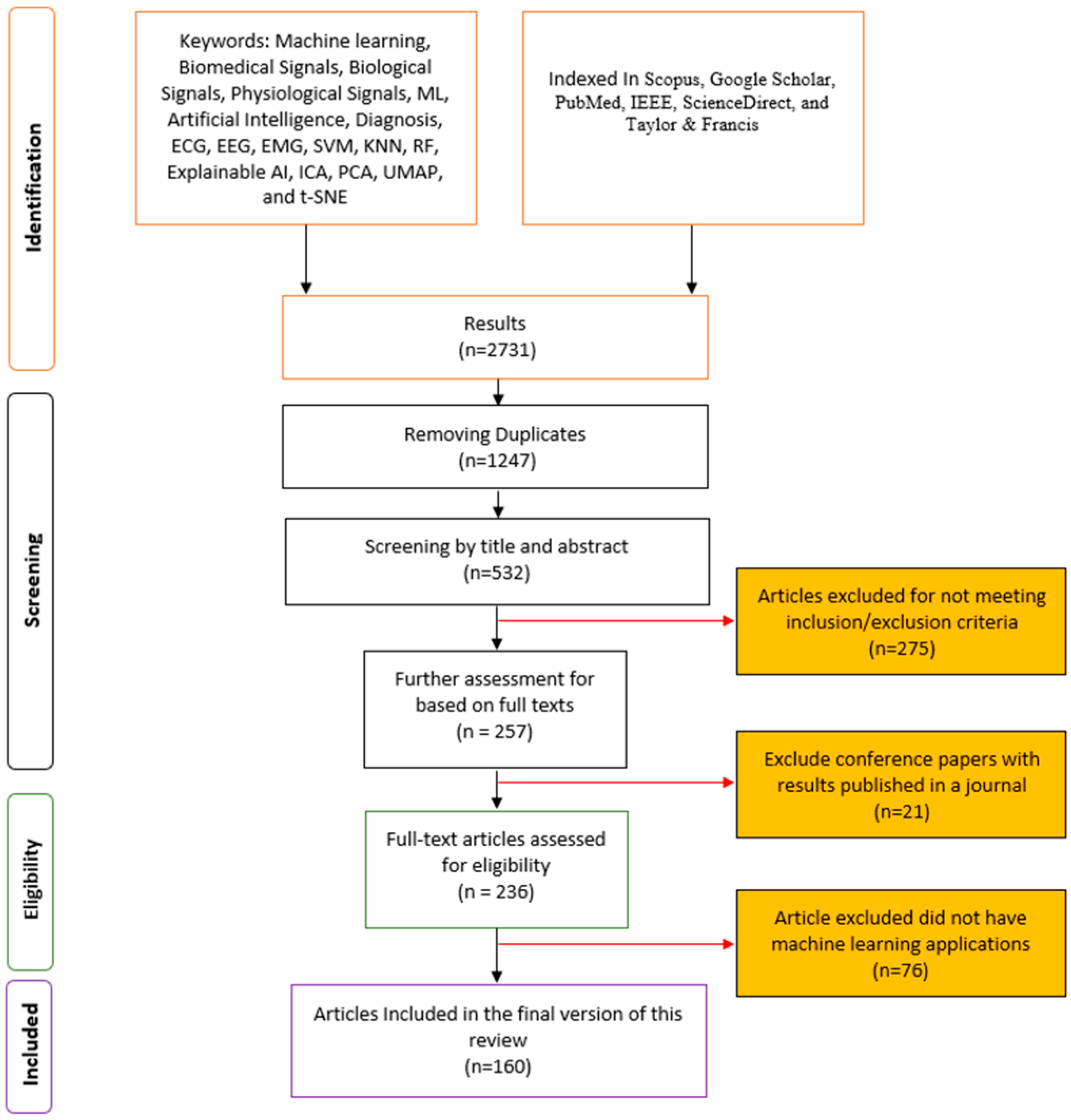
Studies focusing exclusively on deep learning approaches or those that were conference papers without an extended journal publication were generally excluded to maintain the specific scope of this review. A rigorous two-stage screening protocol was implemented to select the most pertinent studies, as depicted in the flowchart in Figure 2.

2.3. Search Keywords and Queries

To ensure the retrieval of highly relevant articles, a combination of keywords spanning three main clusters was utilized:
  • Core ML Terms: Machine learning, ML, Support Vector Machine (SVM), K-Nearest Neighbors (KNN), Artificial Neural Network (ANN), explainable AI, PCA, ICA, UMAP, and t-SNE.
  • Signal Types: biomedical signals, physiological signals, ECG, EEG, EMG, PPG, respiratory sounds, tracheal breathing sounds.
  • Applications: Diagnosis, classification, anomaly detection, real-time monitoring, prognosis, personalized medicine.
  • An example of a search query combining these keywords is: (“machine learning” OR “ML”) AND (“biomedical signals” OR “physiological signals” OR “Biomedical signals” OR “respiratory sounds”) AND (“diagnosis” OR “classification”).
To ensure the retrieval of highly relevant articles, a combination of keywords spanning three main clusters was utilized, as shown in Figure 3.

2.4. Study Selection Process

A rigorous two-stage screening protocol was implemented to select the most pertinent studies:
  • Initial Screening: Articles were initially assessed based on their titles and abstracts. This stage aimed to filter out irrelevant studies and identify potential candidates for full-text review.
  • Full-Text Review: The full texts of the selected articles from the initial screening were thoroughly analyzed to ensure they met all the predefined inclusion criteria. This stage also involved identifying and excluding any duplicate publications or studies that did not align with the focus on traditional ML.

2.5. Bibliometric Analysis

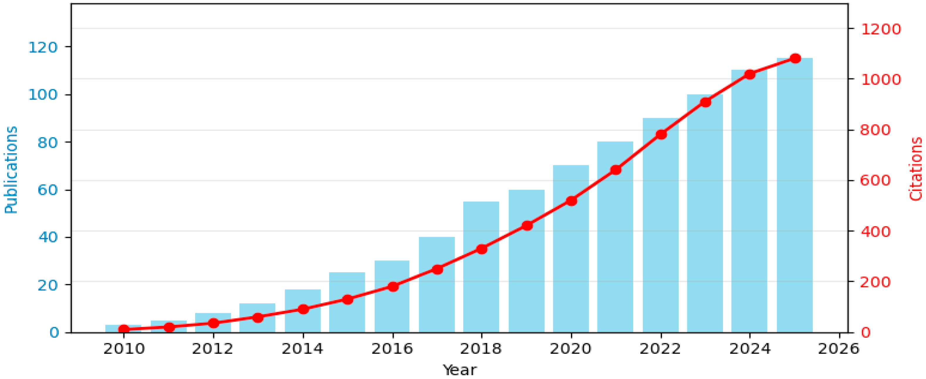
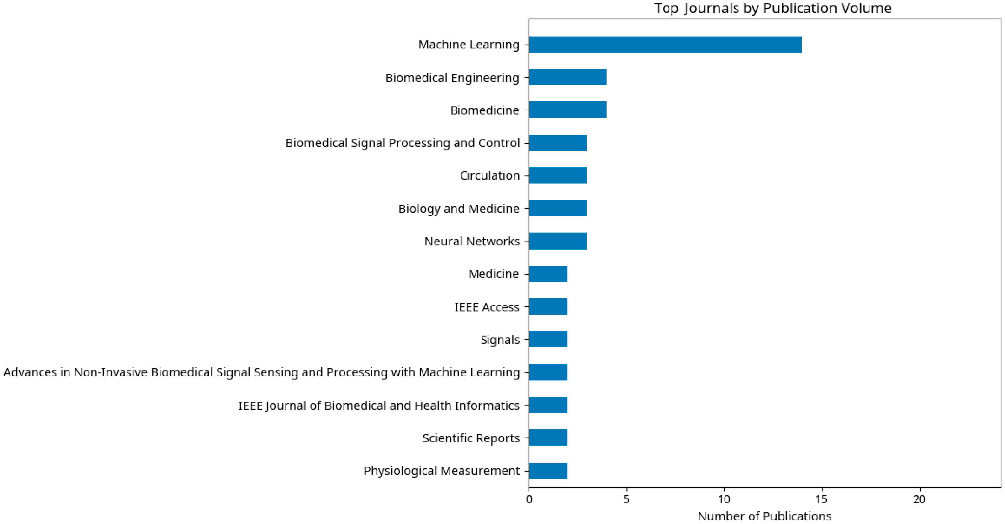
Bibliometric data from the selected studies were analyzed to map research trends and identify key characteristics of the publication landscape in traditional machine learning for biomedical signals. This analysis provides insights into the field’s evolution, prominent publication venues, and scientific output. Figure 4 shows the number of publications over the years.
The analysis of publication years reveals the growth trajectory of research in this domain. As shown in Figure 5, publications on traditional machine learning for biomedical signals have shown a consistent upward trend, indicating increasing academic interest and research activity over the years.

3. ML vs. Deep Learning: Which One Does Serve Better Biomedical Signals?

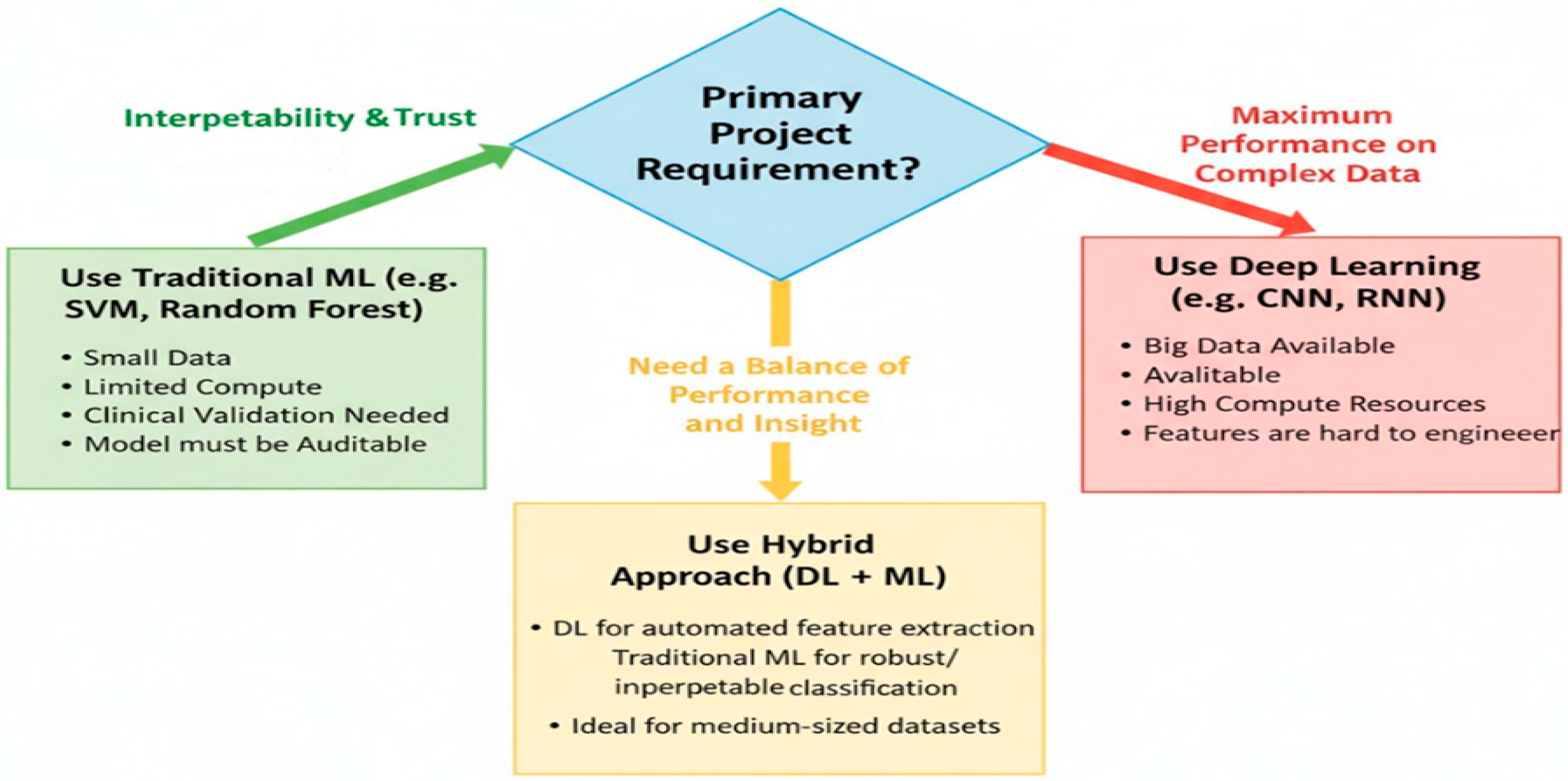
Before delving into the specific methodologies of traditional machine learning (ML), it is essential to understand its unique and often superior value proposition for biomedical signal analysis. While deep learning (DL) has demonstrated remarkable success in domains like image and natural language processing, its application in clinical settings is not always optimal. Traditional ML approaches frequently provide a more practical, robust, and trustworthy solution. This preference is grounded in several critical factors inherent to medical applications: the paramount need for interpretability, the prevalence of small datasets, lower computational costs, the value of domain-informed feature engineering, and alignment with regulatory frameworks. Figure 6 illustrates the flowchart for choosing between ML and DL.

3.1. Superior Interpretability and Transparency for Clinical Trust

The most significant advantage of traditional ML models is their inherent interpretability, a non-negotiable requirement in high-stakes clinical decision-making. Healthcare professionals must understand the reasoning behind a model’s prediction to trust it and incorporate it into patient care [6]. Models like Decision Trees provide explicit decision rules, and Logistic Regression offers apparent feature coefficients indicating the direction and strength of each feature’s influence [7,8]. This transparency allows clinicians to validate the model’s logic against their medical knowledge. In contrast, the “black-box” nature of deep neural networks obscures the decision pathway, posing a significant barrier to clinical adoption and raising ethical concerns [9,10].

3.2. Effectiveness with Limited and Imbalanced Data

Deep learning models are notoriously data-hungry, requiring vast amounts of labeled data to learn effective representations from raw signals without overfitting [2,11]. In medicine, collecting such large, high-quality, and expertly annotated datasets is often prohibitively expensive, time-consuming, and challenged by privacy restrictions. Traditional ML models, operating on carefully engineered features, are far more data-efficient. They can achieve high accuracy with hundreds or thousands of samples rather than the millions needed for DL, making them the only viable option for many specific medical studies [12,13].

3.3. Computational and Operational Efficiency

The training and deployment of deep learning models require significant computational power, often necessitating specialized hardware, such as GPUs. This can be a prohibitive barrier for real-time applications on wearable devices, point-of-care diagnostics, or in resource-limited clinical settings. Traditional ML algorithms, once features are extracted, are computationally lightweight and can run efficiently on standard hardware (CPUs) and even embedded systems [13,14]. This efficiency facilitates faster prototyping, easier deployment, and enables real-time analysis at the bedside.

3.4. The Strategic Advantage of Feature Engineering and Clinical Insight

The requirement for manual feature engineering in traditional ML is a key strategic strength in the medical field. This process requires collaboration between data scientists and clinical experts to ensure that the features are physiologically meaningful. Features like heart rate variability from ECG or specific frequency bands for respiratory sounds are grounded in decades of medical research [15,16,17]. This domain-informed feature set ensures the results are clinically relevant and interpretable, leveraging existing human expertise rather than attempting to learn everything from scratch [18,19].

3.5. Alignment with Regulatory and Ethical Requirements

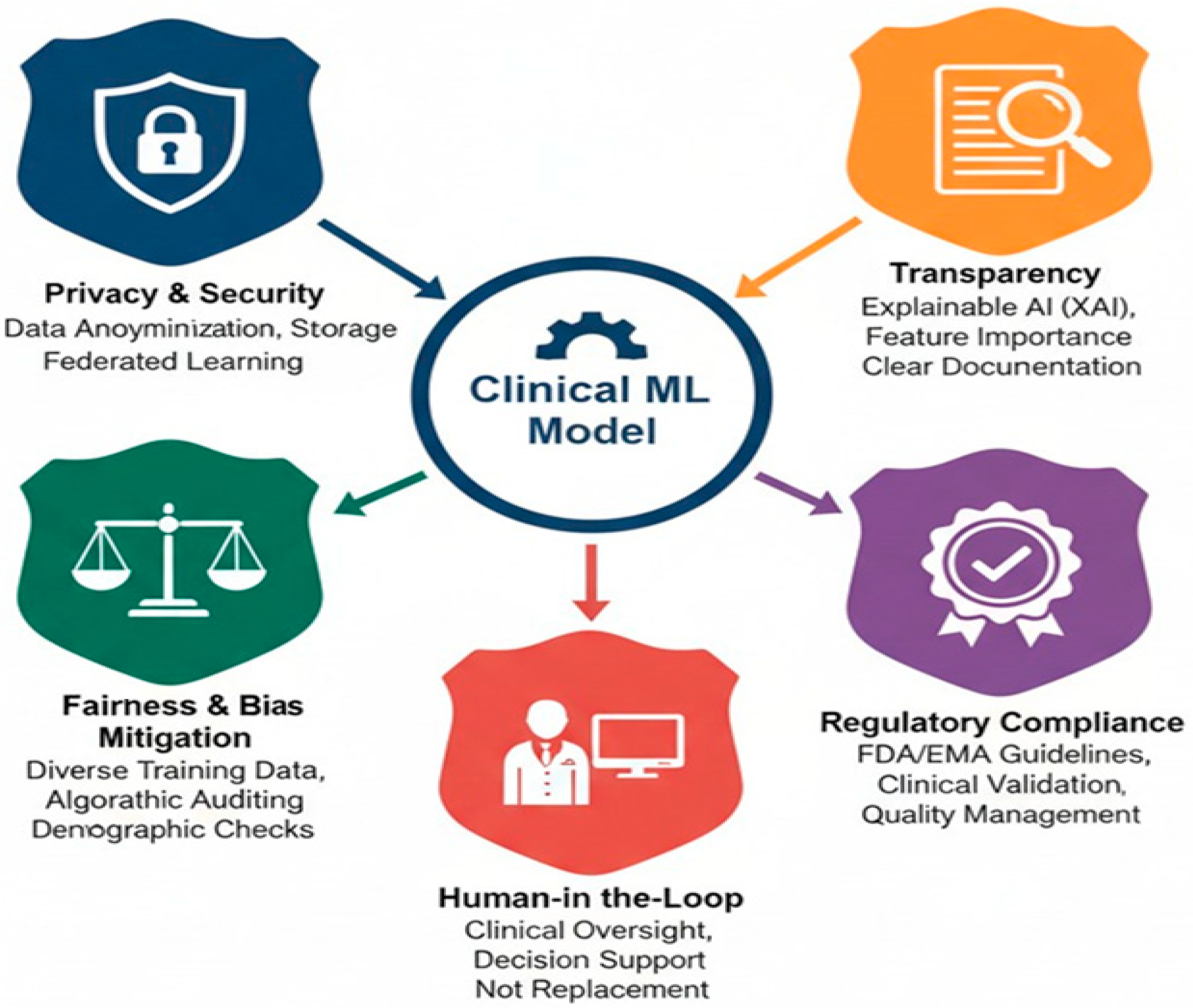
Regulatory approval for AI-driven medical devices (e.g., from the FDA or EMA) requires rigorous evidence of safety, efficacy, and interpretability [20,21]. Traditional ML models are inherently easier to document, audit, and validate due to their simpler architectures and transparent logic. DL models, due to their opacity and complexity, face greater regulatory scrutiny and pose challenges for explaining decisions in the event of an adverse outcome, making the path to clinical certification more arduous [20,21]. Table 1 summarizes the main differences between traditional machine learning and deep learning approaches for biomedical signal analysis.

3.6. Evidence-Based Comparison of ML and DL for Biomedical Signals

While the previous sections qualitatively described the strengths of traditional ML and DL for biomedical signals, it is essential to support these claims with quantitative evidence. Several benchmark studies and systematic reviews have compared the performance, interpretability, and computational efficiency of ML and DL models across different biomedical domains.

3.6.1. Accuracy and Dataset Size

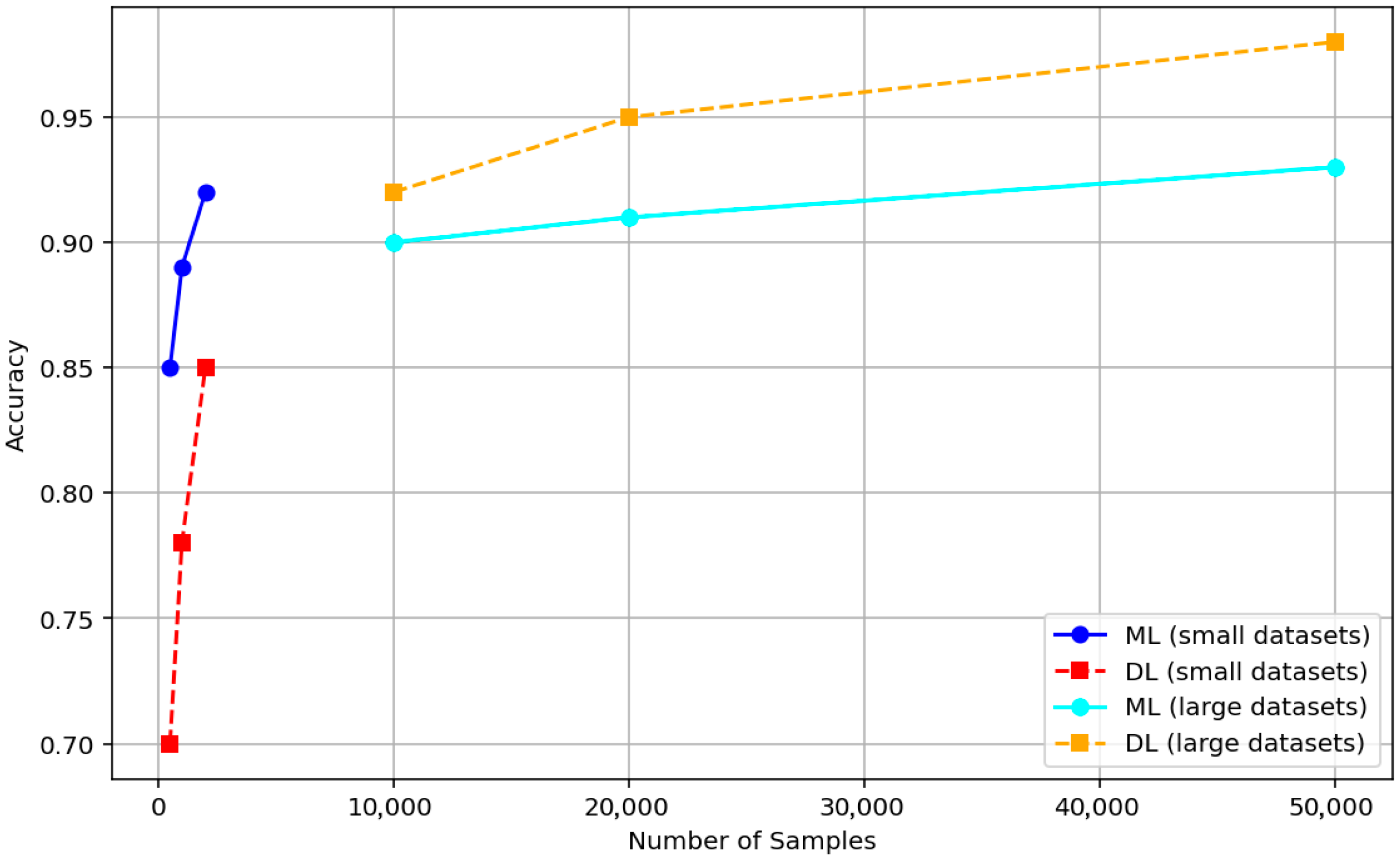
Traditional ML models, including Support Vector Machines (SVM) and Random Forests, generally achieve high accuracy on small-to-medium datasets (<2000 samples). For example, in EMG and ECG signal classification, ML models achieved 85–92% accuracy with datasets containing a few hundred to a few thousand samples, whereas DL models, such as Convolutional Neural Networks (CNNs) or LSTMs, required >10,000 samples to reach comparable performance [22]. Figure 7 shows a tradeoff between dataset size and model accuracy.

3.6.2. Interpretability

Interpretability metrics or proxies, such as the ability to generate feature importance scores or explicit decision rules, consistently favor ML models. Decision Trees and Logistic Regression provide transparent outputs that clinicians can directly evaluate, which is critical for clinician trust. DL models, in contrast, remain largely opaque, with interpretability often requiring post hoc techniques like SHAP or Grad-CAM [23].

3.6.3. Computational Efficiency

ML models are computationally lightweight once features are extracted. For instance, training a Random Forest on 1500 EMG signals took <2 min on a CPU, whereas training a 5-layer CNN on the same dataset required ~8 h on a single GPU to reach similar accuracy [24]. This difference is particularly relevant for real-time monitoring or embedded devices.

3.6.4. Meta-Analytic Evidence

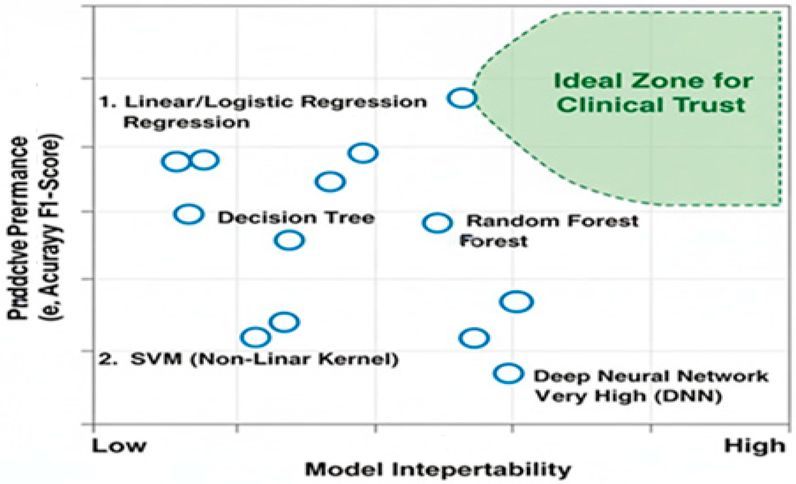
A recent systematic review of 62 studies comparing ML and DL for biomedical signal analysis reported that ML models were preferred in 78% of cases when datasets were small (<5000 samples). DL models outperformed ML primarily in large-scale datasets (>10,000 samples), demonstrating that the choice of methodology should be data-driven [25]. Table 2 highlights the trade-offs between performance and clinical interpretability.

3.7. Research Questions and Identified Gaps

Building on the comparative analysis of traditional ML and DL approaches for biomedical signal analysis, this review is guided by three central research questions:
  • RQ1: Which biomedical signal modalities and feature types are most effectively analyzed using traditional ML versus deep learning, and under what dataset conditions?
  • RQ2: How do current ML methodologies balance predictive performance, interpretability, and clinical applicability, and what are the prevailing gaps in model transparency and regulatory compliance?
  • RQ3: What methodological and validation shortcomings exist in current studies, and how can future research address these gaps to enhance trustworthy and clinically actionable ML solutions?
To systematically summarize these gaps, Table 3 presents a structured overview across key dimensions: signal modality, method, evaluation metric, interpretability, and clinical validation. This framework highlights areas where evidence is sparse, interpretability is limited, or clinical validation is missing, guiding the subsequent discussion of feature engineering, model selection, and case studies.
Overall, the choice between traditional ML and DL is a strategic decision based on the specific clinical problem. While deep learning excels at automating feature extraction from massive datasets, conventional machine learning remains a superior choice for many real-world biomedical signal analysis tasks. Its strengths lie in interpretability, data efficiency, computational simplicity, and the ability to integrate domain knowledge, aligning perfectly with the critical requirements of the medical field: trust, transparency, and practicality. It is within this context that the subsequent discussion of feature engineering, selection, and traditional model interpretation should be understood.

4. Feature Extraction in Biomedical Signal Analysis

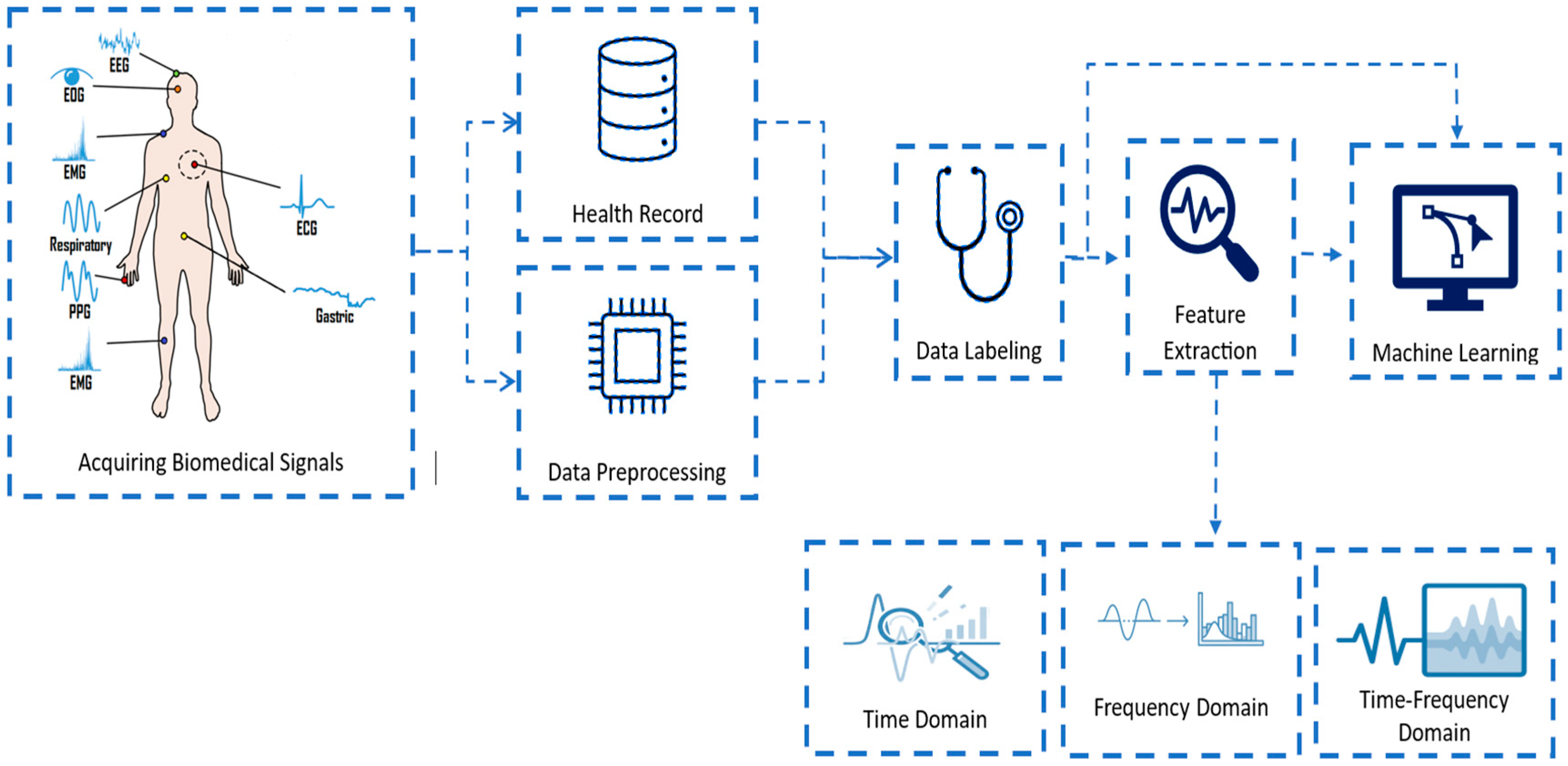
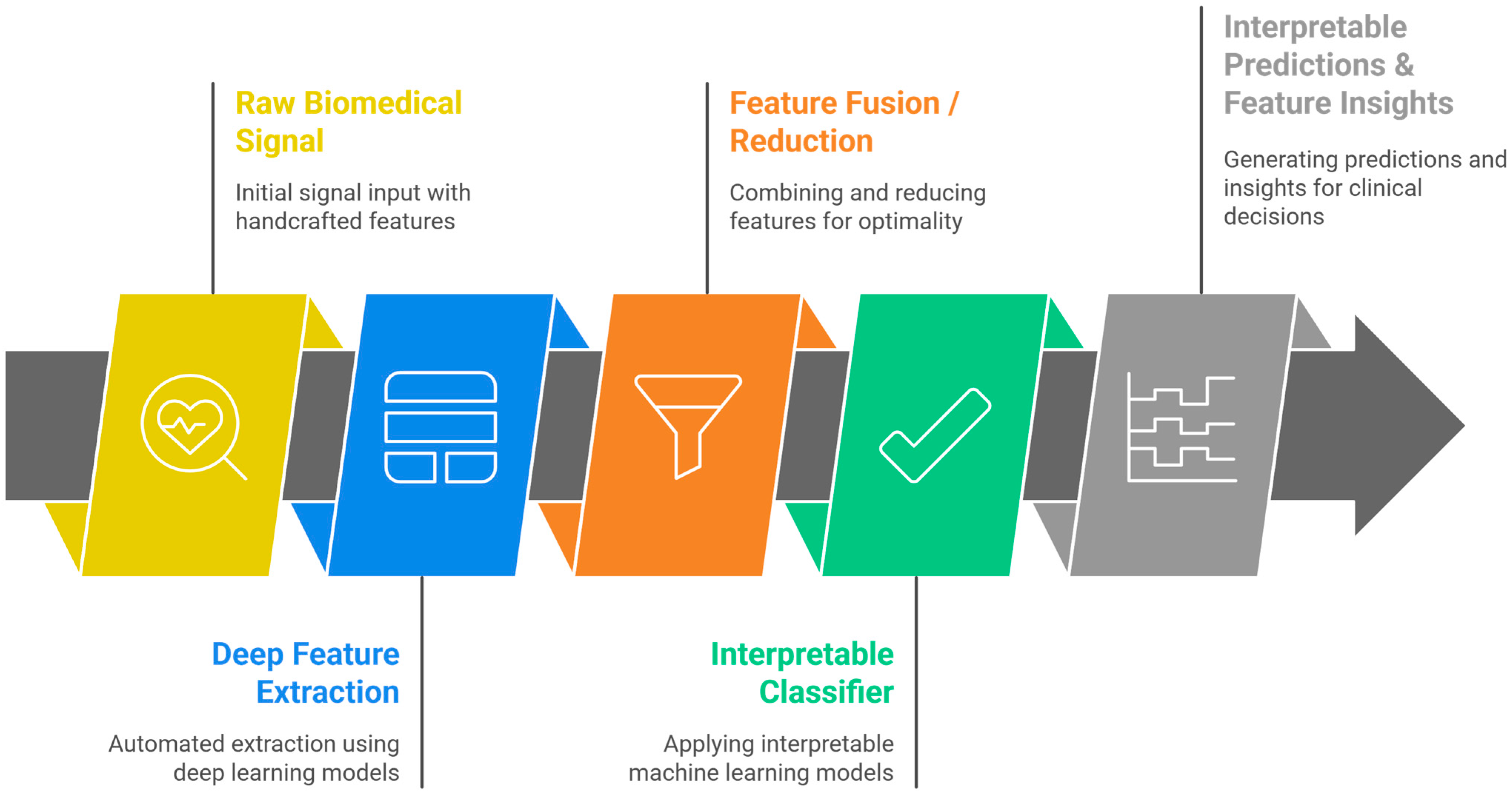
Feature extraction is a fundamental and often the most critical step in applying traditional machine learning algorithms to biomedical signals. It involves transforming raw, high-dimensional signal data into a lower-dimensional set of meaningful and discriminative features. These features should ideally capture the essential characteristics of the signal relevant to the task at hand (e.g., disease diagnosis, activity recognition) while reducing noise and redundancy [18]. The effectiveness of the subsequent ML model heavily depends on the quality and relevance of these extracted features. To improve readability, the following subsections concisely summarize representative feature categories while focusing on their clinical relevance rather than exhaustive mathematical detail. Figure 8 shows the feature extraction process.
Biomedical signals are inherently complex, non-stationary, and often noisy. Therefore, a variety of signal processing techniques are employed to derive features that represent different aspects of the signal. These techniques can be broadly categorized into time-domain, frequency-domain, and time-frequency-domain methods.

4.1. Time-Domain Features

The initial, and often most intuitive, step in characterizing a biomedical signal is extracting time-domain features. These features are computed directly from the raw signal waveform and provide fundamental insights into its amplitude, duration, and morphological structure. Due to their straightforward calculation and interpretability, they serve as a foundational element in the feature engineering pipeline for traditional machine learning. A comprehensive summary of standard time-domain features, their descriptions, and typical applications is provided in Table 4.
Standard time-domain features include:
  • Amplitude-based features: These include maximum, minimum, mean, root mean square (RMS), variance, and standard deviation of the signal. For instance, in EMG signals, RMS is a widely used feature to quantify muscle activity [26]. In tracheal breathing sounds, RMS reflects the power of the signal and is often correlated with the intensity of breathing [27].
  • Morphological features: These describe the shape and characteristics of specific signal components. For ECG, features like P-wave duration, QRS complex duration, ST-segment elevation/depression, and T-wave amplitude are crucial for diagnosing cardiac conditions [28]. In surface EMG, Willison’s Amplitude Algorithm (WAMP) is used to detect muscular activity based on amplitude changes [13].
  • Statistical features: Skewness and kurtosis provide information about the distribution of signal amplitudes. Zero-crossing rate, which counts the number of times the signal crosses the zero axis, can indicate the frequency content or periodicity of the signal and is particularly useful in respiratory sound analysis [29].

4.2. Frequency and Time-Frequency Domains Features

Biomedical signals are inherently non-stationary, meaning their spectral characteristics vary over time. To analyze these signals effectively, it is essential to segment them into short, quasi-stationary windows before applying spectral estimation. Techniques such as the Short-Time Fourier Transform (STFT) or windowed FFT enable estimation of frequency-domain features within these segments, assuming local stationarity. The choice of window length, overlap, and sampling rate is critical to capture transient events while maintaining spectral resolution accurately [30,31,32,33,34]. The primary categories and applications of these features are summarized in Table 5.
Frequency-domain features quantify how the signal’s power is distributed across different frequency bands and are widely applied across biomedical modalities. For example, Power Spectral Density (PSD) can capture dominant frequency bands in EEG (alpha, beta, theta, delta) or ECG-derived heart rate variability. In contrast, band power ratios (e.g., alpha/beta in EEG) can indicate cognitive or pathological states [30,31]. Spectral centroid measures the “center of mass” of the spectrum, providing an overall sense of frequency content [30]. Mel-Frequency Cepstral Coefficients (MFCCs), adapted from speech processing, offer robust representations of tracheal and respiratory sounds that are less sensitive to recording variations [32]. Standard frequency-domain features include:
  • Power Spectral Density (PSD): This measures the signal’s power distribution as a function of frequency. Features derived from PSD include total power in specific frequency bands (e.g., alpha, beta, theta, delta bands in EEG), peak frequency, and spectral edge frequency [30]. In respiratory sounds, specific frequency bands are analyzed for (100–250 Hz) and (300–500 Hz) [31].
  • Spectral Centroid: Represents the center of mass of the spectrum, indicating where the bulk of the frequency content is located [30].
  • Band Power Ratios: Ratios of power in different frequency bands can be highly discriminative, e.g., alpha/beta ratio in EEG for cognitive states [31].
  • Mel-Frequency Cepstral Coefficients (MFCCs): While more common in speech processing, MFCCs have been successfully applied to tracheal breathing sounds for their ability to capture the spectral envelope, which is robust to variations in recording conditions [32].
Time-frequency methods extend this analysis by providing a joint representation of spectral content evolution over time, which is critical for detecting transient or oscillatory phenomena that may be missed in purely frequency-domain approaches. Wavelet transforms (both continuous and discrete) decompose the signal into frequency components at multiple resolutions, allowing feature extraction such as energy, entropy, and statistical moments from specific wavelet sub-bands [30,33]. STFT, on the other hand, produces a spectrogram representing frequency content over time, from which features like time-varying power or dominant frequencies can be computed [34]. Combining frequency-domain and time-frequency features enhances the ability to characterize complex biomedical signals such as EEG, ECG, and respiratory sounds. Standard time-frequency domain features include:
  • Wavelet Transform (WT): The Discrete Wavelet Transform (DWT) and Continuous Wavelet Transform (CWT) decompose a signal into different frequency components at various resolutions [33]. Features can be extracted from the wavelet coefficients, such as energy, entropy, and statistical moments within specific wavelet sub-bands [30]. Wavelet analysis is effective for capturing both transient and oscillatory phenomena in signals like ECG and EEG.
  • Short-Time Fourier Transform (STFT): While less flexible than wavelets, STFT provides a spectrogram, which is a visual representation of the signal’s frequency content over time. Features can be extracted from the spectrogram, such as changes in power or dominant frequencies over specific time windows [34].

4.3. Advanced Time-Frequency Representations

Beyond standard STFT and Wavelet Transforms, advanced time-frequency representations, such as the Wigner-Ville Distribution or the Hilbert-Huang Transform (HHT), can provide sharper time-frequency localization and are particularly suited for analyzing non-stationary and non-linear signals. Features extracted from these representations can offer richer insights into the dynamic changes within biomedical signals [35].
These advanced feature engineering techniques, when judiciously applied, can significantly enhance the discriminative power of traditional ML models, enabling them to uncover subtle patterns and relationships in biomedical signals that are critical for accurate diagnosis, prognosis, and monitoring [17].

4.4. Multi-Scale Feature Extraction

Biomedical phenomena often manifest across multiple temporal and spatial scales. Multi-scale feature extraction techniques aim to capture information at different resolutions. For instance, multi-scale entropy analyzes signal complexity across various scales, providing a more comprehensive understanding than single-scale entropy measures. Wavelet-based features, as discussed earlier, inherently offer a multi-scale perspective, but further advanced multi-scale approaches can be developed to optimize feature representation for specific tasks [36,37,38].

4.5. Non-Linear Features

Biomedical signals frequently exhibit non-linear and chaotic behavior, which can be indicative of underlying physiological states or pathologies. Non-linear features aim to quantify this complexity. Examples include:
  • Chaos Theory Features: Measures like Lyapunov exponents, correlation dimension, and fractal dimension can characterize the chaotic dynamics of signals such as heart rate variability (HRV) and electroencephalogram (EEG). These features provide insights into the regularity and predictability of the system [39,40].
  • Entropy Measures: Various entropy measures (e.g., Sample Entropy, Approximate Entropy, Permutation Entropy) quantify the regularity or irregularity of a time series. Lower entropy often indicates more predictable or regular patterns, while higher entropy suggests greater complexity or randomness. These are widely used in EEG for seizure detection and sleep stage classification, and in ECG for assessing cardiac health [16,36].

4.6. Higher-Order Statistics (HOS)

While traditional features often rely on first and second-order statistics (mean, variance, power spectrum), Higher-Order Statistics (HOS) provide information about the non-Gaussianity and non-linearity of a signal. HOS, such as bispectrum and trispectrum, can detect phase coupling and non-linear interactions that are invisible to power spectrum analysis. They are handy for analyzing non-linear systems and detecting transient events in signals like EEG and evoked potentials [41,42,43].

4.7. Automated Feature Engineering via Bio-Inspired Algorithms

Bio-inspired optimization algorithms (e.g., genetic algorithms, particle swarm optimization) offer a promising avenue for automating feature extraction and selection. These methods iteratively evolve feature subsets or transformation parameters to maximize model performance, reducing reliance on manual feature engineering. For example, genetic algorithms have optimized wavelet parameters for ECG arrhythmia detection, improving classification accuracy by 8–12% compared to standard wavelet features [44,45,46]. Similarly, particle swarm optimization has enhanced feature selection for EMG-based gesture recognition, minimizing redundancy while preserving discriminative power [47]. Integrating these techniques with traditional ML pipelines can accelerate model development and adapt to signal-specific characteristics, such as non-stationarity in respiratory sounds or EEG artifacts.

4.8. Other Feature Extraction Techniques

Beyond the primary domains, other methods are employed for specialized feature extraction:
  • Statistical Features: Higher-order statistics (e.g., bispectrum, trispectrum) can capture non-linear relationships and non-Gaussian properties in signals that are not evident from second-order statistics (like power spectrum).
  • Non-linear Dynamics and Chaos Features: For signals exhibiting chaotic or fractal properties, features like Lyapunov exponents, correlation dimension, and fractal dimension can be extracted. These are particularly relevant in EEG analysis for understanding brain states [48].
  • Principal Component Analysis (PCA) and Independent Component Analysis (ICA): While primarily dimensionality reduction techniques, PCA and ICA can also be used for feature extraction by transforming the original signal into a new set of uncorrelated (PCA) or statistically independent (ICA) components, which can then serve as features [49]. ICA is effective for removing artifacts from EEG signals.
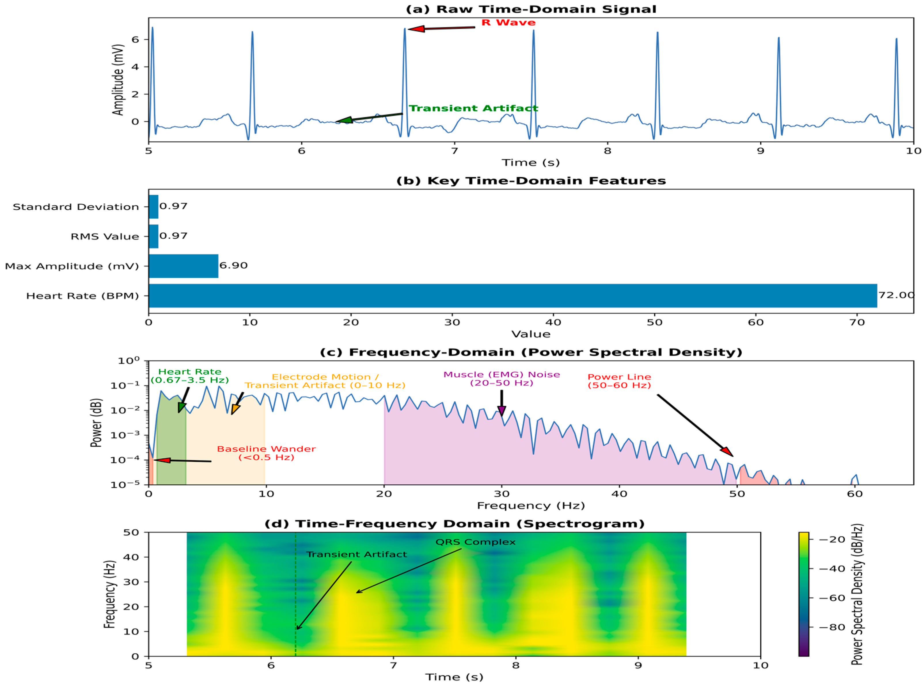
The choice of feature extraction technique depends heavily on the type of biomedical signal, the specific clinical question, and the characteristics of the underlying physiological phenomena. Practical feature engineering is paramount for the success of traditional ML models, as it directly influences their ability to learn and generalize from the data. Figure 9 illustrates the ECG signal across multiple domains: time, frequency, and time, clearly identifying the QRS complex and transient artifacts.

5. Feature Selection for Enhanced Model Performance

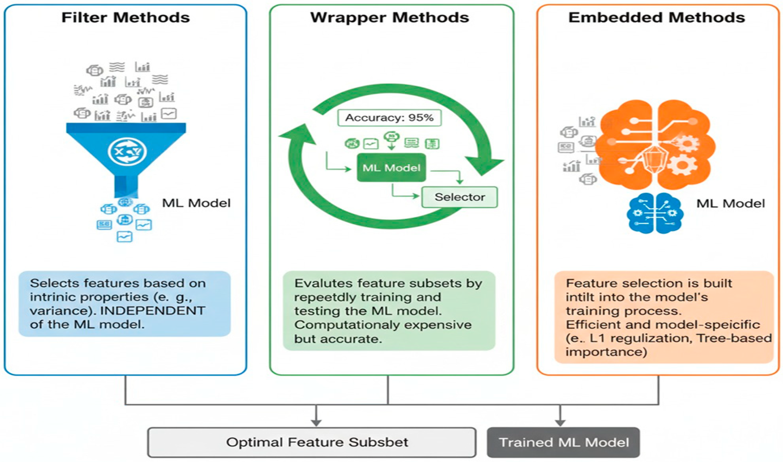
After extracting a comprehensive set of features from biomedical signals, the next crucial step in traditional machine learning pipelines is feature selection. Feature selection aims to identify and select a subset of the most relevant, non-redundant, and informative features for model training. This process is vital for several reasons: it reduces dimensionality, mitigates overfitting, improves model interpretability, and often enhances computational efficiency and predictive performance [50,51]. Figure 10 summarizes the feature selection process.
In biomedical signal analysis, where datasets can be high-dimensional, noisy, and limited in sample size, effective feature selection improves generalization only when combined with unbiased testing, such as cross-validation and strict train-test separation, preventing data leakage. Irrelevant features add noise, increase computational cost, and reduce performance on unseen data. Feature selection methods can be broadly categorized into three types: filter methods, wrapper methods, and embedded methods. Different feature selection methods offer distinct approaches to identifying the most relevant features, as outlined in Table 6.

5.1. Filter Methods

Filter methods select features based on their intrinsic properties, such as correlation with the target variable or statistical significance, regardless of the chosen machine learning algorithm. These methods are computationally efficient and can be used as a preprocessing step. Standard filter methods include:
  • Variance Threshold: Removes features with very low variance, as they carry little information.
  • Correlation-based Feature Selection (CFS): Selects features that are highly correlated with the class but lowly correlated with each other [52].
  • Statistical Tests: Uses statistical measures like the Chi-squared test, the ANOVA F-value, or mutual information to assess the relationship between each feature and the target variable. Features with higher statistical scores are preferred [53].

5.2. Wrapper Methods

Wrapper methods evaluate subsets of features by training and testing a machine learning model on each subgroup. These methods tend to be more accurate than filter methods because they consider the interaction between the features and the chosen learning algorithm. However, they are computationally more expensive due to the need to train the model multiple times. Standard wrapper methods include:
  • Forward Selection: This starts with no features and adds at each step the feature that results in the highest model performance increase.
  • Backward Elimination: It starts with all available features and removes the least important in a systematic way until the performance of the model begins to degrade.
  • Recursive Feature Elimination (RFE): recursively trains the model, at each iteration removing features with the lowest importance score to get a subset of desired features [54].

5.3. Embedded Methods

Embedded methods perform feature selection as an integral part of the model training process. These methods combine the advantages of both filter and wrapper methods, offering a balance between computational efficiency and accuracy. Examples include:
  • Lasso (L1 Regularization): Adds a penalty term to the loss function that forces some feature coefficients to become exactly zero, effectively performing feature selection [55].
  • Tree-based Methods: Algorithms like Decision Trees, Random Forests, and Gradient Boosting Machines inherently perform feature selection by assigning importance scores to features based on how much they contribute to reducing impurity or error in the tree construction [56]. For instance, in the context of surface EMG signal classification, Random Forests and Decision Trees are suitable for feature selection and classification tasks, aiding in identifying key respiratory signal characteristics [13].
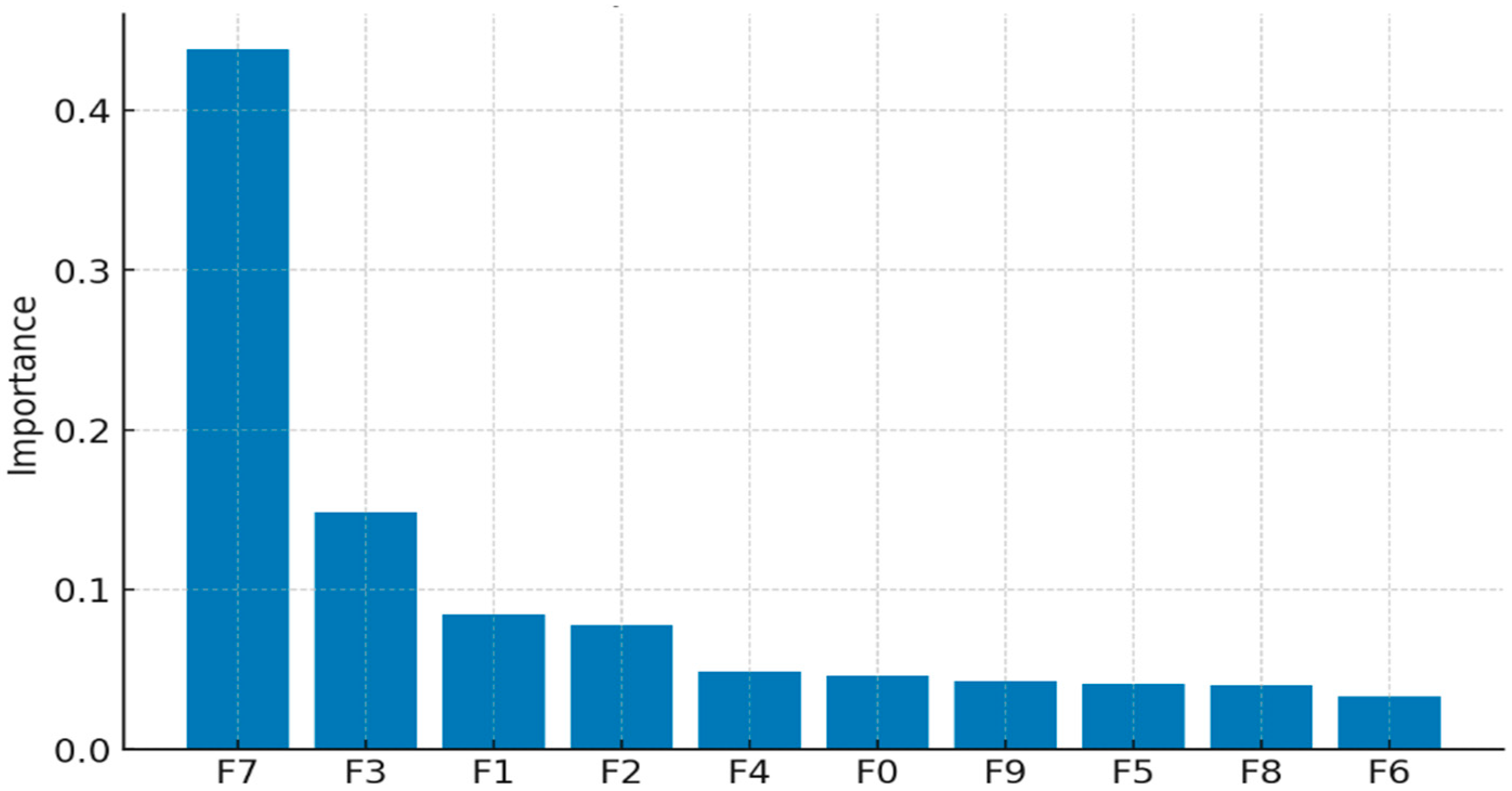
The choice of feature selection method often depends on dataset size, feature type, and the specific ML algorithm being used. A well-executed feature selection process can significantly enhance the performance, interpretability, and generalizability of traditional ML models in biomedical signal analysis. Figure 11 shows a sample output of feature selection using random forests.

6. Machine Learning Algorithms for Biomedical Signals Classification

Traditional ML algorithms have been widely applied to biomedical signal analysis due to their interpretability, computational efficiency, and effectiveness in various diagnostic and classification tasks [3]. These algorithms, unlike deep learning models, operate on handcrafted features, making the decision-making process more transparent. This section discusses some of the most commonly used traditional ML algorithms and their applications in biomedical signal processing. A variety of conventional machine learning algorithms are employed for biomedical signal analysis, each with distinct characteristics and optimal use cases, as compared in Table 7.

6.1. Linear Classifiers

Linear classifiers are a family of algorithms that assume that data points can be separated into distinct classes by a linear decision boundary, such as a line (in 2D), a plane (in 3D), or a hyperplane (in higher dimensions). These models are computationally efficient and interpretable, making them suitable for biomedical applications where explainability is crucial [57].

6.1.1. Logistic Regression

Logistic Regression is one of the most widely used linear models for binary classification. It predicts the probability of a categorical outcome by applying a logistic (sigmoid) function to a linear combination of input features. Its simplicity and interpretability make it highly suitable for clinical applications where understanding feature contribution is essential [58,59].
  • Applications: Used for disease prediction based on biomedical signals, such as ECG-based arrhythmia detection and classification of normal versus abnormal respiratory sounds [60].
  • Performance: Performs well when the relationship between predictors and targets is approximately linear but may underperform on complex, non-linear datasets without appropriate feature transformations.

6.1.2. Linear Discriminant Analysis (LDA)

Linear Discriminant Analysis (LDA) is a statistical classifier that models the distribution of features for each class and finds a linear combination that maximizes class separability. It assumes that classes share the same covariance matrix [61].
  • Applications: Applied in EEG-based emotion recognition, brain–computer interface (BCI) control, and ECG classification [61], EVestG for detecting post-concussion syndrome with and without comorbid depression [62,63].
  • Performance: Highly interpretable and practical for low-dimensional, linearly separable data but performance decreases when class distributions deviate from Gaussian assumptions.

6.1.3. Perceptron

The Perceptron is one of the earliest neural-inspired classifiers, learning a linear decision boundary by iteratively adjusting weights based on classification errors. It serves as a foundational model for modern neural networks [64].
  • Applications: Early biomedical uses include binary classifications such as abnormal ECG beat detection and differentiation of breathing states [64].
  • Performance: Effective for linearly separable data but inadequate for complex, non-linear problems. Modern extensions, such as Multi-Layer Perceptrons, address these limitations.

6.2. Probabilistic Classifiers

Probabilistic classifiers apply principles of probability to predict class membership, often providing interpretable results and fast computation [64].

6.2.1. Naïve Bayes

Naïve Bayes is a probabilistic classifier based on Bayes’ theorem, assuming independence among input features. It calculates the posterior probability of each class given the observed data and assigns the class with the highest probability. Its simplicity and computational efficiency make it highly practical for biomedical signal analysis [60].
  • Applications: Naïve Bayes has been applied to real-time disease detection systems, EEG-based emotion recognition, and classification of respiratory and cardiovascular abnormalities in high-dimensional biomedical datasets [60].
  • Performance: Performs efficiently even with limited training data and high-dimensional inputs, but its independence assumption may reduce accuracy when features are strongly correlated.

6.2.2. Gaussian Mixture Models (GMMs)

Gaussian Mixture Models (GMMs) classify data by modeling each class as a weighted combination of multiple Gaussian distributions, capturing complex underlying feature distributions in biomedical signals [65].
  • Applications: GMMs have been used for speaker and breathing sound classification, sleep stage identification, and modeling variability in ECG and PPG signal patterns [65].
  • Performance: Provide flexible modeling of non-linear and multi-modal data distributions but can be sensitive to initialization and may converge to local optima without proper parameter tuning.

6.3. Support Vector Machines (SVMs)

Support Vector Machines (SVMs) are robust supervised learning algorithms designed to handle both classification and regression problems. They work by identifying the optimum hyperplane that separates data points belonging to different classes in a high-dimensional feature space. In biomedical signal analysis, SVMs provide particular advantages, since they handle high-dimensional datasets effectively and demonstrate strong resistance to overfit-ting even on limited training datasets [3].
  • Applications: SVMs have been successfully applied in various biomedical signal processing tasks, including:
    • ECG Classification: Detecting cardiac arrhythmias [66].
    • EEG Classification: Identifying different brain states or detecting epileptic seizures [67].
    • EMG Classification: Recognizing muscle movements or diagnosing neuromuscular disorders [24].
    • Respiratory Sound Classification: Classifying normal and abnormal breathing patterns in tracheal sounds [68].
    • EVestG for classification of alzheimer’s patients with mixed pathology [69,70].
  • Performance: SVMs often achieve high accuracy, especially when combined with appropriate kernel functions (e.g., Radial Basis Function (RBF) kernel) that can capture non-linear relationships in the data. Their performance is highly dependent on the quality of the extracted features.

6.4. Instance-Based Classifiers

These “lazy” learners make predictions based on similarity to previously observed data rather than building an explicit global model [71].

K-Nearest Neighbors (KNN)

K-Nearest Neighbors (KNN) is one of the simplest, non-parametric, and instance-based learning algorithms for classification and regression tasks. It labels a new data point with the majority class of its ‘k’ nearest neighbors in the feature space. KNN is one of the most frequently used initial approaches in biomedical signal analysis due to its simplicity and ease of implementation [71].
  • Applications: KNN has been used for:
    • ECG Classification: Identifying normal and abnormal heartbeats [72].
    • EEG Classification: Classifying sleep stages [73].
    • Respiratory Sound Analysis: Initial classification of breathing patterns [74].
  • Performance: KNN’s performance is sensitive to the choice of ‘k’ and the distance metric used. It can be computationally expensive for large datasets during the prediction phase, as it requires calculating distances to all training samples. It is also sensitive to irrelevant features, highlighting the importance of effective feature selection.

6.5. Tree-Based Classifiers

Tree-based classifiers form one of the most interpretable and versatile families of machine learning algorithms used in biomedical signal analysis. They operate by recursively partitioning the feature space into decision regions, producing a hierarchical tree structure that maps input features to class outcomes through explicit if–then rules [75]. This transparency allows clinicians and researchers to trace predictions back to physiological features, making these models particularly suitable for applications demanding explainability. Moreover, ensemble extensions such as Random Forests and Gradient Boosting significantly enhance predictive performance and robustness, mitigating overfitting while maintaining interpretability key requirements for reliable biomedical diagnostics and monitoring [75].

6.5.1. Decision Trees

Decision trees are a versatile, non-parametric, and widely used family of supervised learning algorithms applicable to both classification and regression problems. They work by recursively partitioning the data into subsets based on feature values, eventually generating a hierarchical, tree-like structure that represents a series of decision rules. The intuitive interpretability of this structure makes them an attractive approach that is also useful for discovering key patterns and relationships within biomedical data [75].
  • Applications: Widely used for respiratory sound classification [76], EEG-based sleep stage identification [77], and interpretable disease diagnosis from biomedical features [78].
  • Performance: Highly interpretable but prone to overfitting on noisy data unless pruned or regularized.

6.5.2. Random Forests

Random Forests represent a strong ensemble learning technique that builds multiple decision trees during the training process and aggregates their outputs using the mode for classification tasks or the mean for regression tasks. Combining several trees’ predictions, this approach enhances model stability, reduces overfitting, and improves generalization performance compared to individual decision trees. Random Forests have proven remarkably successful in analyzing complex, high-dimensional biomedical datasets [75].
  • Applications: Common in respiratory pathology classification, sleep disorder analysis, and general biomedical diagnostic systems [75].
  • Performance: Offer high accuracy, robustness to noise, and feature-importance measures that enhance interpretability.

6.5.3. Gradient Boosting Machines (GBM)

Gradient Boosting Machines build trees sequentially, each correcting errors from prior ones using gradient-based optimization [79].
  • Applications: Used in disease prediction, ECG classification, and respiratory sound analysis [79].
  • Performance: Achieve strong accuracy on complex datasets but require careful hyperparameter tuning to prevent overfitting.

6.5.4. XGBoost and LightGBM

XGBoost and LightGBM are optimized gradient boosting frameworks offering parallelization and regularization enhancements [80].
  • Applications: Extensively applied biomedical classification tasks with structured or tabular data [80].
  • Performance: Deliver superior computational efficiency and predictive accuracy compared with conventional GBM.

6.6. Ensemble and Boosting Methods

Boosting algorithms improve model performance by combining multiple weak learners (usually shallow decision trees) into a single, strong predictive model. These ensemble methods are potent in biomedical signal classification, where feature interactions are often complex and non-linear.

6.6.1. AdaBoost (Adaptive Boosting)

AdaBoost works by sequentially training a series of weak classifiers, each focusing more on the samples misclassified by previous ones. The final model is a weighted sum of these weak learners [77,81].
  • Applications: AdaBoost has been applied to various biomedical signal classification tasks, including sleep stage identification from EEG, respiratory sound pathology detection, and cardiovascular disease prediction [77,81].
  • Performance: Offers high accuracy and robustness to overfitting when tuned properly but can be sensitive to noisy data and outliers since misclassified samples are given higher weights in subsequent rounds.

6.6.2. CatBoost (Categorical Boosting)

CatBoost is a gradient boosting algorithm specifically designed to handle categorical features efficiently, reducing the need for extensive preprocessing. It uses ordered boosting and permutation-driven techniques to prevent overfitting and improve generalization [82].
  • Applications: CatBoost has been used in biomedical contexts such as multimodal disease prediction (combining anthropometric, physiological, and acoustic features) and respiratory sound analysis [82].
  • Performance: Demonstrates strong performance even on small and heterogeneous biomedical datasets. Compared to other boosting algorithms like XGBoost and LightGBM, CatBoost provides better handling of categorical data and often superior interpretability through feature importance scores.

6.7. Neural Network-Based Classifiers

Although shallow ANNs are sometimes grouped under traditional ML, they bridge the gap toward deep learning by modeling non-linear relationships between inputs and outputs.

Artificial Neural Networks (ANNs)

Artificial Neural Networks (ANNs) are a class of powerful, non-linear supervised learning models inspired by the structure and function of the biomedical brain. They consist of interconnected layers of nodes (neurons) that process input data by learning hierarchical representations through adjustable connection weights. ANNs are universal function approximators, capable of modeling complex, non-linear relationships between inputs and outputs, making them highly versatile for both classification and regression tasks [83].
  • Applications: These algorithms are extensively applied in biomedical signal processing for:
    • Respiratory Sound Classification: Extracting complex patterns from audio signals to detect wheezing, crackles, and other pathological sounds with high precision [84].
    • Sleep Stage Classification: Processing multimodal data (EEG, EOG, EMG) to automatically classify sleep stages with performance rivaling human experts [85].
    • Disease Diagnosis: Serving as the foundation for complex deep learning models that analyze images (e.g., MRI, X-ray), signals (e.g., ECG, EEG), and genetic data for diagnostic decision support [86].
  • Performance: ANN with many layers can achieve state-of-the-art accuracy on complex tasks by automatically learning relevant features from raw or minimally processed data. However, they often require large amounts of training data, are computationally intensive, and can act as “black boxes,” making their decisions less interpretable than those of tree-based models [57]. Techniques like dropout and regularization are commonly used to mitigate overfitting.

6.8. Hybrid and Meta-Model Approaches

Hybrid and Meta-Model Approaches integrate multiple machine learning classifiers to leverage their complementary strengths and improve predictive accuracy and robustness. Instead of relying on a single algorithm, these methods combine outputs from diverse models, such as linear, tree-based, probabilistic, and neural network classifiers, using strategies like stacking, blending, or weighted ensembling [87,88]. In stacking, for instance, base learners generate individual predictions that are then used as input features for a higher-level “meta-learner,” which refines the final decision. Weighted ensembles, by contrast, assign importance to each model based on its performance metrics, such as sensitivity or specificity, allowing for more balanced diagnostic outcomes [87,88].
  • Applications: Hybrid and meta-model frameworks have been widely adopted in biomedical signal processing, where data are often heterogeneous and non-linear. They have been successfully applied in respiratory sound classification, sleep stage detection, cardiovascular disease diagnosis, and multimodal fusion of anthropometric, physiological, and acoustic features. By combining classifiers optimized for different modalities, these approaches enhance generalizability and reduce bias associated with single-model predictions [87,88].
  • Performance: Meta-models consistently outperform individual classifiers in terms of accuracy, sensitivity, and specificity, particularly in complex biomedical datasets. They offer robustness against noise and inter-subject variability while maintaining adaptability to new data distributions. However, their effectiveness depends on careful selection and weighting of base learners, and the interpretability of the final model can be more challenging than that of standalone algorithms.
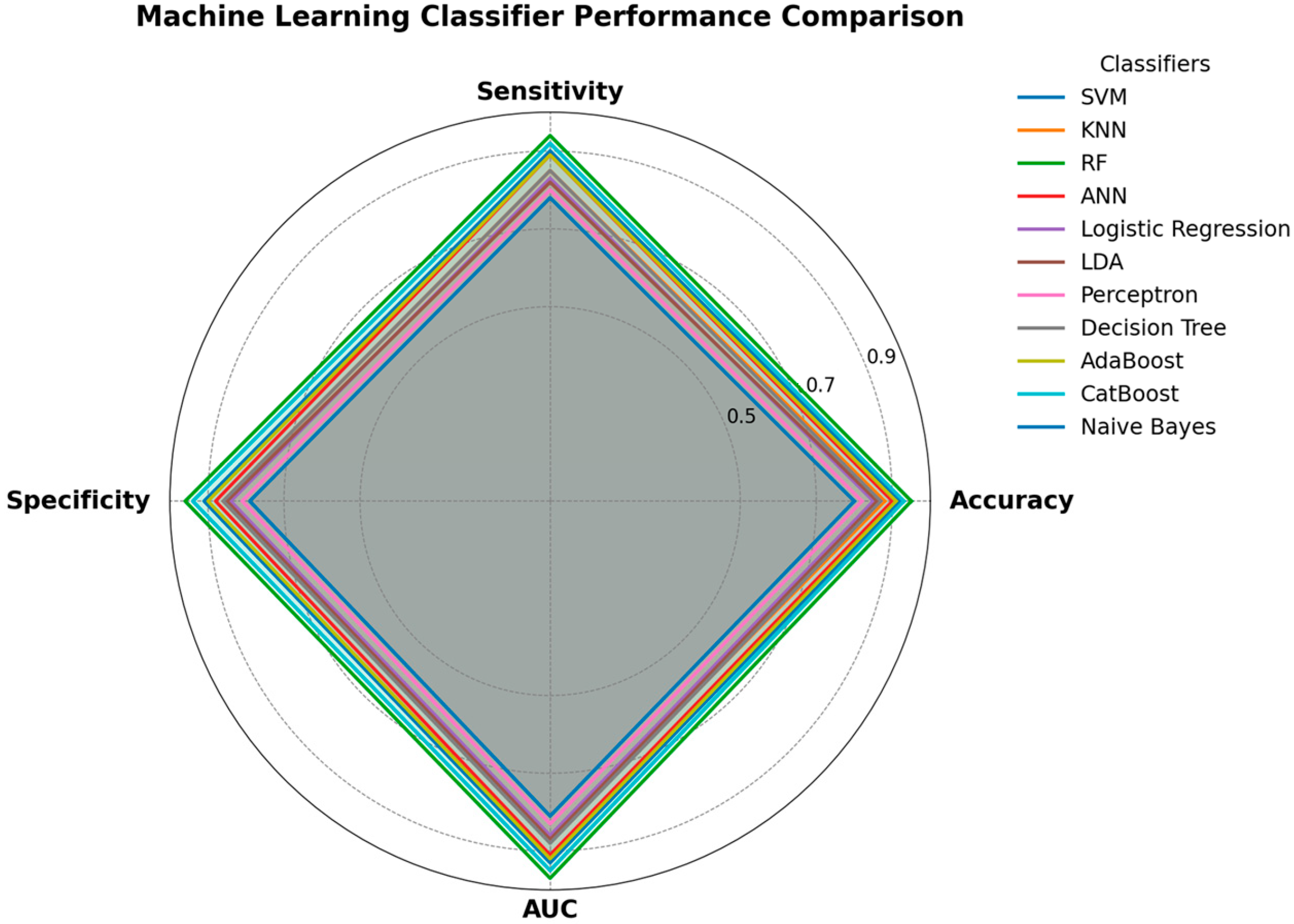
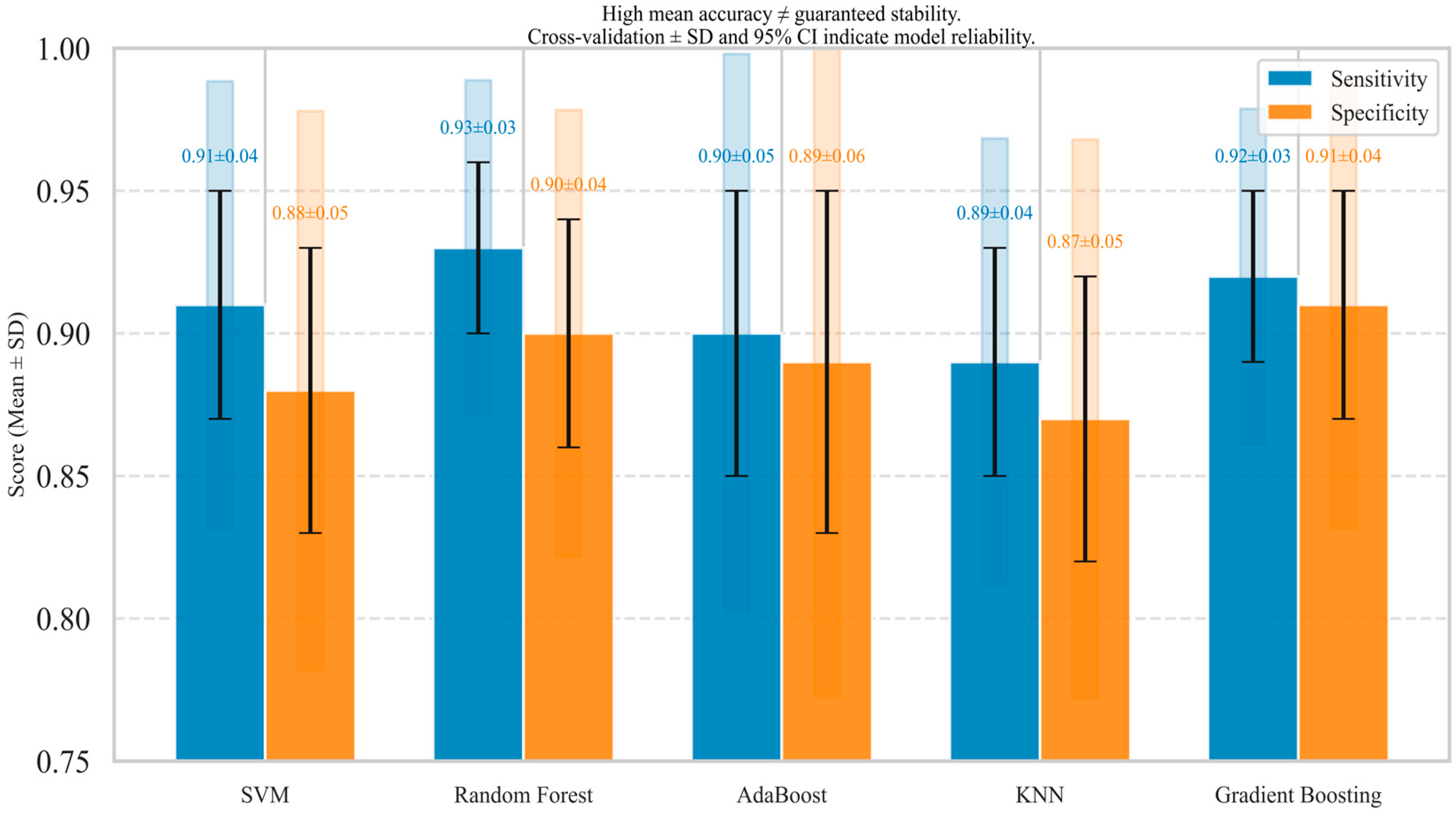
The choice of a traditional ML algorithm depends on the specific characteristics of the biomedical signal data, the nature of the problem (classification, regression), and the desired trade-off between model complexity, performance, and interpretability. Often, a comparative analysis of several algorithms is performed to identify the most suitable one for a given application. Figure 12 compares different metrics across varying ML algorithms.

7. Ensuring Unbiased Testing and Model Validation

In biomedical signal analysis, reliable testing and validation are essential for assessing a model’s genuine predictive performance. Many reported improvements in classification accuracy result from biased evaluation protocols such as using overlapping data for both training and testing which lead to inflated results and poor generalization to unseen data [50,58,60]. To prevent this, testing must be conducted on data that remain completely independent from those used during model development, feature selection, or hyperparameter tuning [51,52].
The most fundamental safeguard is data separation into distinct training, validation, and testing subsets. The training set is used to fit model parameters, the validation set guides feature and parameter optimization, and the test set provides an independent measure of generalization [53,54]. This separation eliminates circular evaluation and ensures that model performance reflects true predictive ability rather than memorization of training patterns [55].
Cross-validation strategies, such as k-fold, stratified, or leave-one-subject-out validation, are particularly valuable for biomedical datasets that are small or imbalanced [56,57,58]. These methods average performance across multiple train–test splits, reducing the influence of random sampling bias and improving reliability. Subject-independent validation ensuring that signals from the same participant do not appear in both training and testing subsets is especially critical for physiological studies, where within-subject consistency can artificially inflate accuracy [59,60].
Beyond internal validation, blind testing on external datasets or data collected under different conditions provides the most rigorous assessment of model generalizability and clinical readiness [61,64]. Such testing demonstrates whether a model can adapt to unseen subjects, sensors, or recording environments an essential criterion for clinical translation [65].

7.1. Example of Subject-Independent Data Separation and External Testing

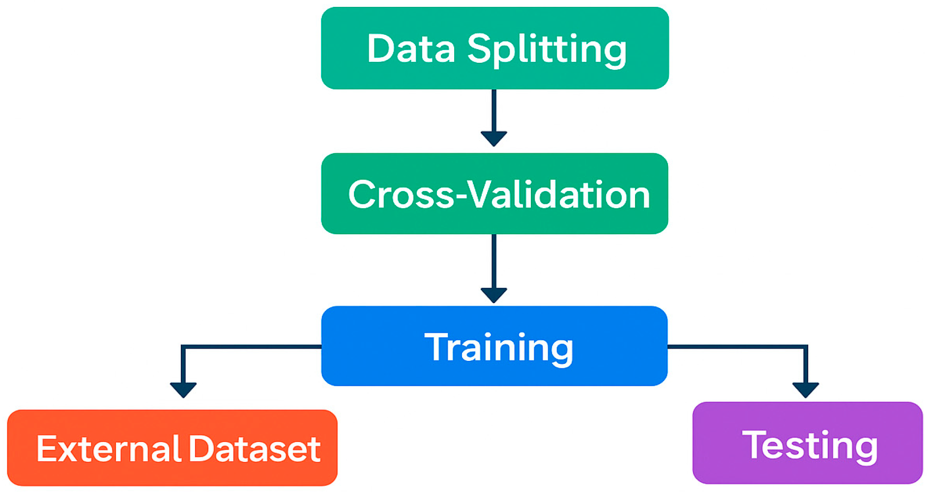
A robust evaluation protocol combines subject-independent internal validation with external testing on independent datasets. For example, in tracheal breathing sound analysis, a leave-one-subject-out (LOSO) cross-validation can be applied, where all recordings from a single participant are reserved for testing while the remaining subjects form the training set. This ensures that the model does not encounter any data from the test subject during training, preventing inflated performance metrics. To further assess generalizability, the trained model can then be evaluated on an external dataset collected under different conditions or at a separate clinical site. This approach demonstrates both subject-independent performance and adaptability to unseen environments, providing a rigorous assessment of model reliability, clinical readiness, and real-world applicability. Figure 13 shows subject-independent data separation and the external testing flow chart.

7.2. Data Standardization and Harmonization for Reproducible ML Pipelines

The reproducibility and clinical translation depend on how consistently you handle your data. In biomedical research, even small differences in data processing can completely change your results. Many times, signals vary in sampling rate, amplitude range, and sensor quality. Without harmonization, comparability across studies or research centers can’t be performed. Consistent handling isn’t just good practice; it is the foundation of scientific trust. The following points are how to make your data reliable and comparable:
  • Preprocess and normalize signals: Use a common sampling rate and normalize amplitudes using z-score or percentile scaling, in such a way that differences in sensor sensitivity or recording conditions do not distort your analyses [51,52].
  • Document metadata: Record acquisition settings, sensor specifications, subject demographics and clinical labels in open formats such as BIDS [61,64]. Good documentation lets others understand exactly how and where your data came from.
  • Normalization across Subjects: Subject-independent normalization will avoid leakage and improve generalization of the data [59,60]. This way, your model stays honest when new patients are introduced.
  • Make workflows reproducible: by storing preprocessing scripts and trained models in open repositories such as GitHub or Zenodo. Always use fixed random seeds to be reproducible by others [53,54].
  • Apply FAIR (Findable, Accessible, Interoperable and Reusable) data principles: Make your data Findable, Accessible, Interoperable and Reusable. FAIR data practices extend the life of your work and help others build on it.
This will make your results more than numbers; they become reliable evidence others can trust and build on. Transparent data handling enables benchmarking fairly, supports multi-center collaboration, and allows your models to move from research labs into clinical use. In the end, reproducibility is what turns your machine learning pipeline into a clinically meaningful tool. Finally, ensuring transparent reporting of evaluation protocols including data partitioning, randomization, cross-validation schemes, and comprehensive performance metrics (e.g., sensitivity, specificity, AUC) is vital for reproducibility and fair comparison across studies [24,66,67]. Together, these best practices establish the foundation of unbiased testing, enabling the development of machine-learning models that are not only accurate but also trustworthy and clinically meaningful [68].

8. Dimensionality Reduction & Feature Projection Methods

High-dimensional biomedical data often contain redundant or correlated features that may obscure the underlying patterns relevant for classification. Dimensionality reduction and feature projection techniques aim to transform data into a lower-dimensional space while retaining the most informative characteristics. These methods improve computational efficiency, reduce overfitting, and enhance the interpretability of models. In biomedical signal analysis, they are particularly valuable for simplifying complex feature sets derived from spectral, temporal, and statistical domains [89,90,91,92,93].

8.1. Principal Component Analysis (PCA)

Principal Component Analysis (PCA) is one of the most widely used linear dimensionality reduction methods. It projects the data onto a new coordinate system such that the first few principal components capture the maximum variance in the data. PCA assumes linear relationships among features and is computationally efficient [90].
  • Applications: PCA has been extensively used in biomedical signal processing for EEG denoising, ECG beat classification, and feature selection in respiratory sound analysis [90].
  • Performance: It enhances classifier performance by removing collinear features and noise but may lose discriminative information when class separability is non-linear.

8.2. Independent Component Analysis (ICA)

Independent Component Analysis (ICA) separates mixed signals into statistically independent components by maximizing non-Gaussianity. Unlike PCA, which focuses on variance, ICA seeks statistical independence among components [89].
  • Applications: ICA is commonly applied in EEG artifact removal (e.g., separating eye-blink or muscle noise from neural activity), as well as in respiratory and phonocardiogram signal separation [89].
  • Performance: Effective in source separation and artifact removal; however, it may suffer from instability if the number of sources is unknown or when applied to small datasets.

8.3. Linear Discriminant Analysis (LDA) for Feature Projection

Although primarily a classifier, LDA can also serve as a supervised projection method, reducing dimensionality by maximizing class separability. It projects data onto a lower-dimensional space that best discriminates between classes [94].
  • Applications: LDA-based projection has been used for feature extraction in voice pathology detection, EEG-based emotion recognition, and sleep stage classification [95].
  • Performance: More effective than PCA when class labels are available but assumes Gaussian-distributed classes with equal covariance matrices.

8.4. Non-Linear Manifold Learning Methods

Non-linear techniques capture intrinsic, curved structures in data that linear projections like PCA and LDA cannot represent. These methods are particularly useful for complex biomedical signals exhibiting non-linear dependencies.
  • t-Distributed Stochastic Neighbor Embedding (t-SNE): Focuses on preserving local relationships between data points, making it highly effective for visualization of clusters (e.g., disease vs. healthy subjects) [96].
  • Uniform Manifold Approximation and Projection (UMAP): Provides faster computation and better preservation of both local and global data structures compared to t-SNE [97].
  • Applications: Both methods are widely used for visualizing high-dimensional representations in EEG, EMG, and deep-learning-derived feature spaces [98,99].
  • Performance: Excellent for exploration data analysis and visualization, but generally unsuitable as preprocessing for traditional classifiers due to non-deterministic mappings.

8.5. Autoencoders for Non-Linear Feature Compression

Autoencoders are shallow neural networks trained to reconstruct input data while compressing information through a low-dimensional latent space. They represent a bridge between feature extraction and deep learning [91,92].
  • Applications: Autoencoders have been applied for unsupervised feature learning from respiratory, cardiac, and EEG signals, often improving downstream classification performance [91,92].
  • Performance: Capable of learning complex, non-linear representations; however, they require sufficient data and careful regularization to avoid overfitting.
High-dimensional biomedical data often contain redundant or correlated features that may obscure the underlying patterns relevant for classification. Dimensionality reduction and feature projection techniques aim to transform data into a lower-dimensional space while retaining the most informative characteristics. These methods improve computational efficiency, reduce overfitting, and enhance model interpretability. In biomedical signal analysis, they are particularly valuable for simplifying complex feature sets derived from spectral, temporal, and statistical domains. Figure 14 shows an example of dimensionality reduction methods applied to biomedical signal features with two classes.

9. Interpretation of Traditional Machine Learning Models

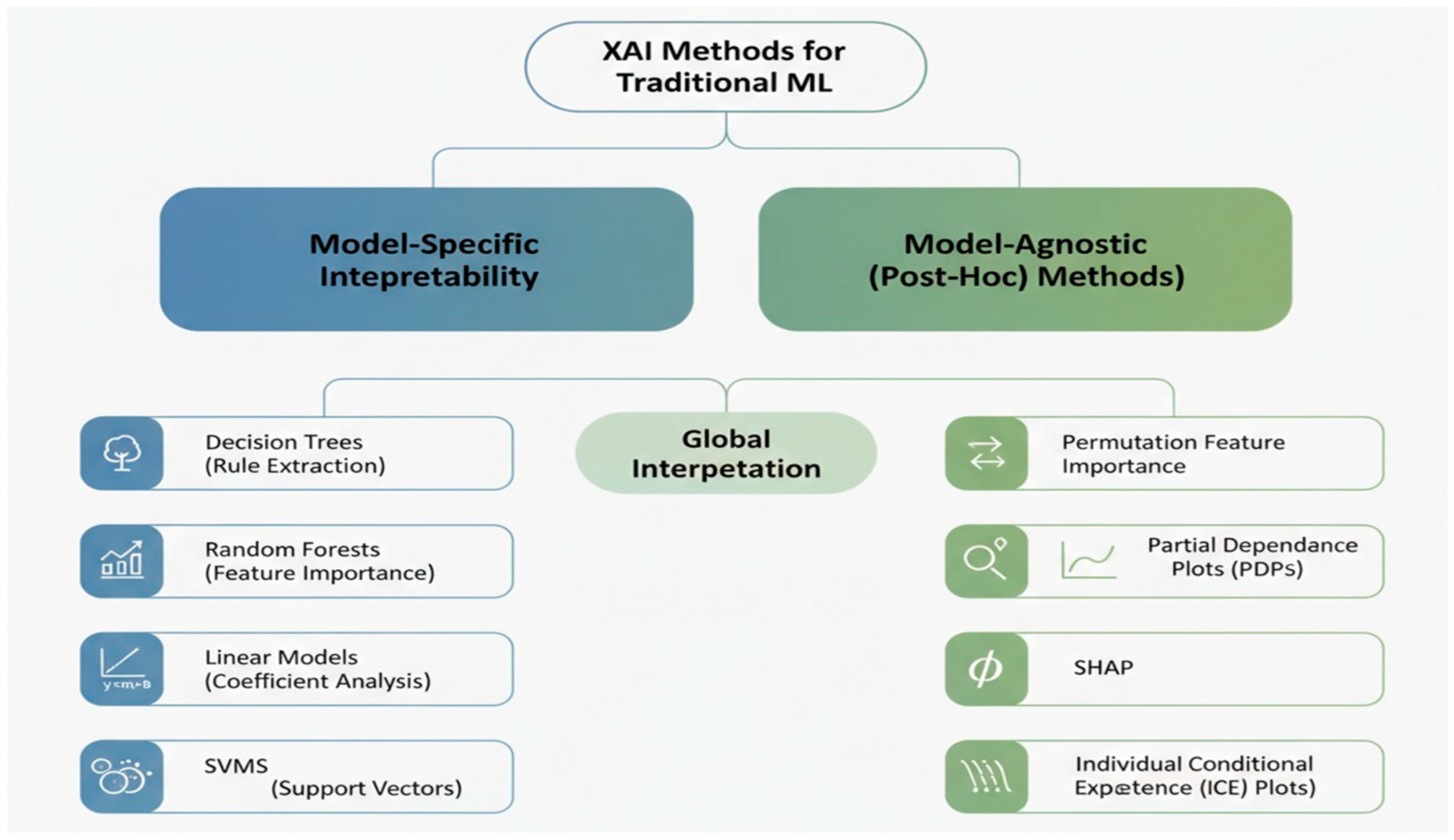
Interpretability is a crucial aspect of machine learning models, especially in high-stakes domains like healthcare, where understanding the rationale behind a model’s prediction is as important as the prediction itself. Traditional machine learning models often offer greater interpretability than their deep learning counterparts, primarily because of their simpler architectures and reliance on handcrafted features. This section explores methods for interpreting traditional ML models in the context of biomedical signal analysis. Throughout this review, interpretability refers to the ability to comprehend model reasoning; explainability denotes post hoc analytical techniques; and transparency describes the overall clarity and trustworthiness of a model in clinical contexts. Together, these qualities ensure practical applicability, clinical trust, and meaningful insight without excessive repetition of any single term. These distinctions ensure consistent terminology and avoid redundancy. Figure 15 shows the explainable methods in ML.

9.1. Model-Specific Interpretability

Many traditional ML algorithms inherently provide insights into their decision-making process:
  • Decision Trees: These models are inherently interpretable as they represent a series of explicit rules. The path from the root to a leaf node provides a clear explanation for a specific prediction. Feature importance can also be directly derived from how often and how early a feature is used to split the data [100]. In biomedical applications, decision trees can provide clinically meaningful rules, such as “if RMS > 0.5 and spectral centroid < 800 Hz, then classify as abnormal breathing.”
  • Random Forests: While an ensemble of many decision trees can be less straightforward to visualize than a single tree, Random Forests still provide feature importance scores. These scores indicate the relative contribution of each feature to the overall predictive power of the model, often calculated based on the decrease in impurity (e.g., Gini impurity) or accuracy when a feature is used for splitting [61].
  • Support Vector Machines (SVMs): For linear SVMs, the weights assigned to each feature can indicate their importance. Features with larger absolute weights have a greater influence on the decision boundary. For non-linear SVMs with kernel tricks, direct interpretation of feature weights is more challenging, but techniques like examining support vectors can provide some insight into critical data points [64].
  • Logistic Regression: As a linear model, logistic regression provides coefficients for each feature. The sign and magnitude of these coefficients indicate the direction and strength of the relationship between the feature and the log-odds of the target variable, making it highly interpretable [59].

9.2. Post Hoc Interpretability Methods

Even for traditional models, or when a more global understanding of feature importance is needed across different model types, post hoc methods can be applied:
  • Permutation Feature Importance: This model-agnostic technique measures the importance of a feature by calculating the increase in the model’s prediction error after permuting the feature’s values. A significant increase in error indicates that the feature is essential [101]. This method is beneficial for comparing feature importance across different model types. Figure 16 shows a sample feature of the importance of plot.
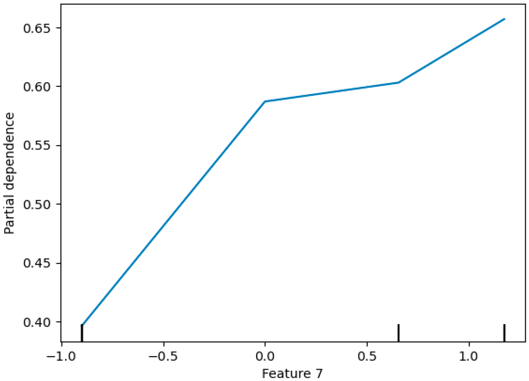
  • Partial Dependence Plots (PDPs): PDPs show the marginal effect of one or two features on the predicted outcome of a machine learning model. They illustrate how the prediction changes as the feature value varies, while other features are averaged out [102,103]. In biomedical signal analysis, PDPs can show how changes in specific signal characteristics (e.g., spectral centroid) affect the probability of a particular diagnosis. Figure 17 shows a sample partial dependence plot.
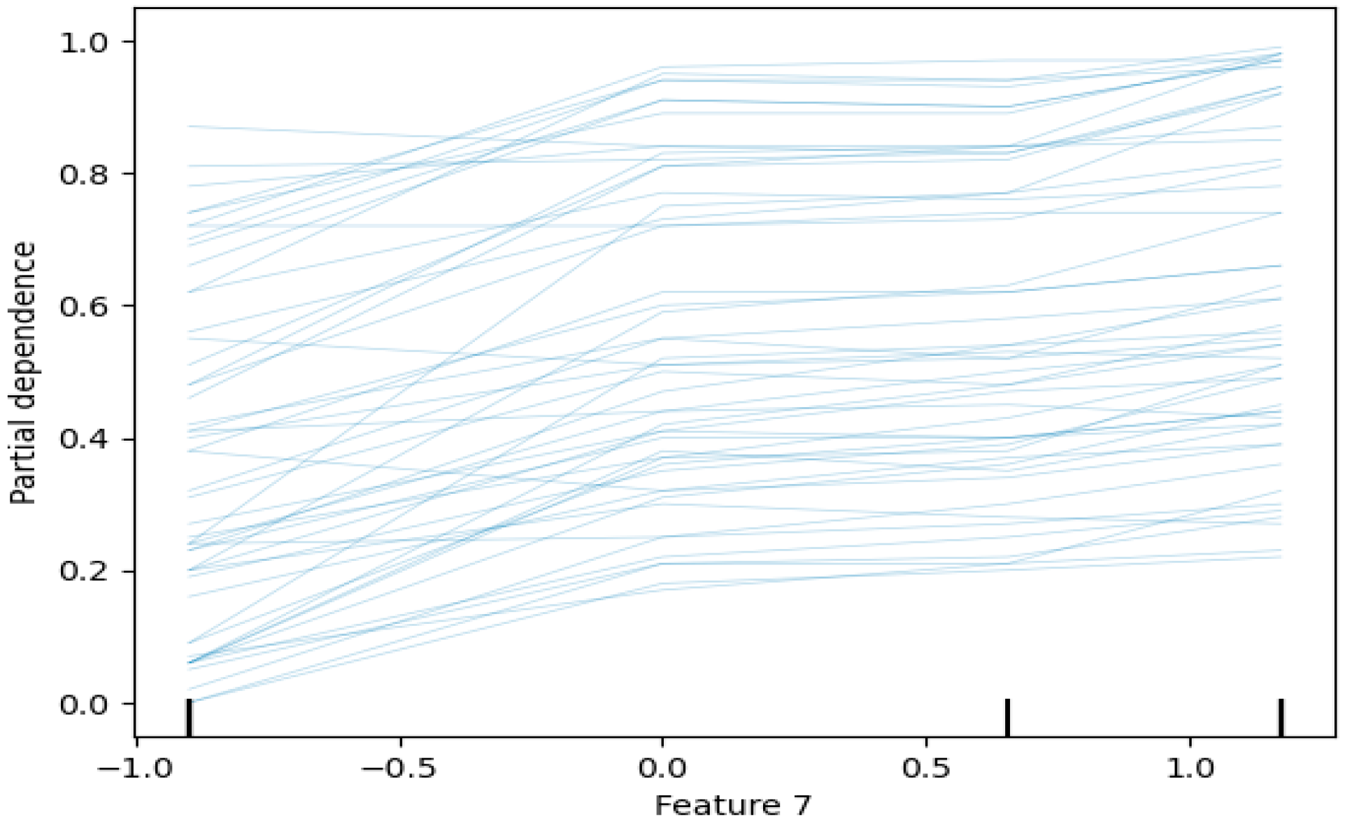
  • Individual Conditional Expectation (ICE) Plots: Similarly to PDPs, ICE plots show the dependence of the prediction on a feature for each instance separately, revealing heterogeneous relationships that might be obscured by averaging in PDPs [104]. Figure 18 shows a sample ICE plot.
  • SHAP (SHapley Additive exPlanations): SHAP values quantify the contribution of each feature to a model’s prediction using concepts from cooperative game theory. They provide both global and local interpretability, showing how individual features drive predictions for specific instances and across the entire dataset [105,106]. SHAP is particularly useful in biomedical signal analysis to understand which signal characteristics most strongly influence diagnostic outcomes. Figure 19 shows a sample of the SHAP values plot.
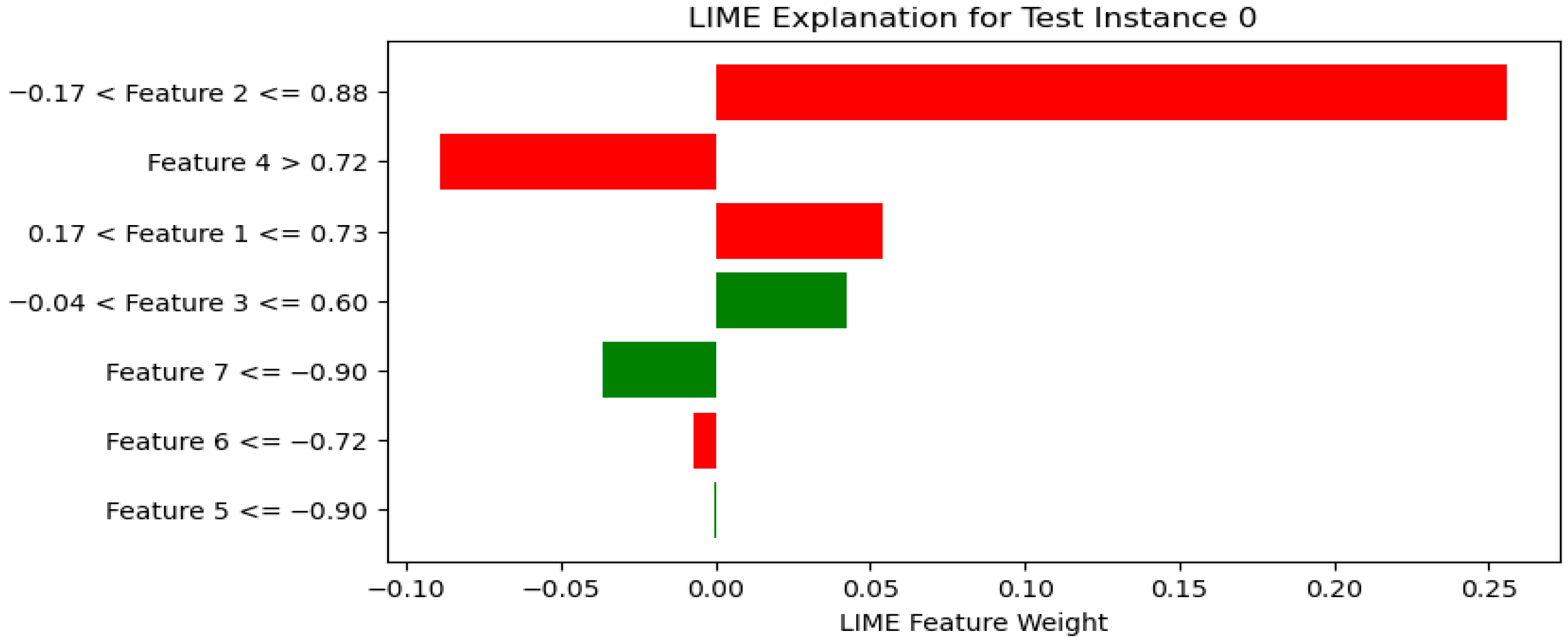
  • LIME (Local Interpretable Model-agnostic Explanations): LIME approximates complex models locally with interpretable surrogate models (e.g., linear models) to explain individual predictions. By perturbing input features and observing the changes in predictions, LIME identifies which features are most influential for a specific instance [107]. This method helps clinicians understand model decisions for individual patients without requiring complete model transparency. Figure 20 shows a sample LIME plot.

9.3. Visualization for Interpretation

Visualizing features and model outputs is critical for interpretation:
  • Feature Distribution Plots: Histograms, box plots, and violin plots can show the distribution of individual features and how they differ across classes. These visualizations can reveal which features are most discriminative and whether there are clear separations between different conditions [108].
  • Scatter Plots and Pair Plots: These can reveal relationships between pairs of features and their correlation with the target variable. In biomedical signal analysis, scatter plots might show the relationship between time-domain and frequency-domain features [109].
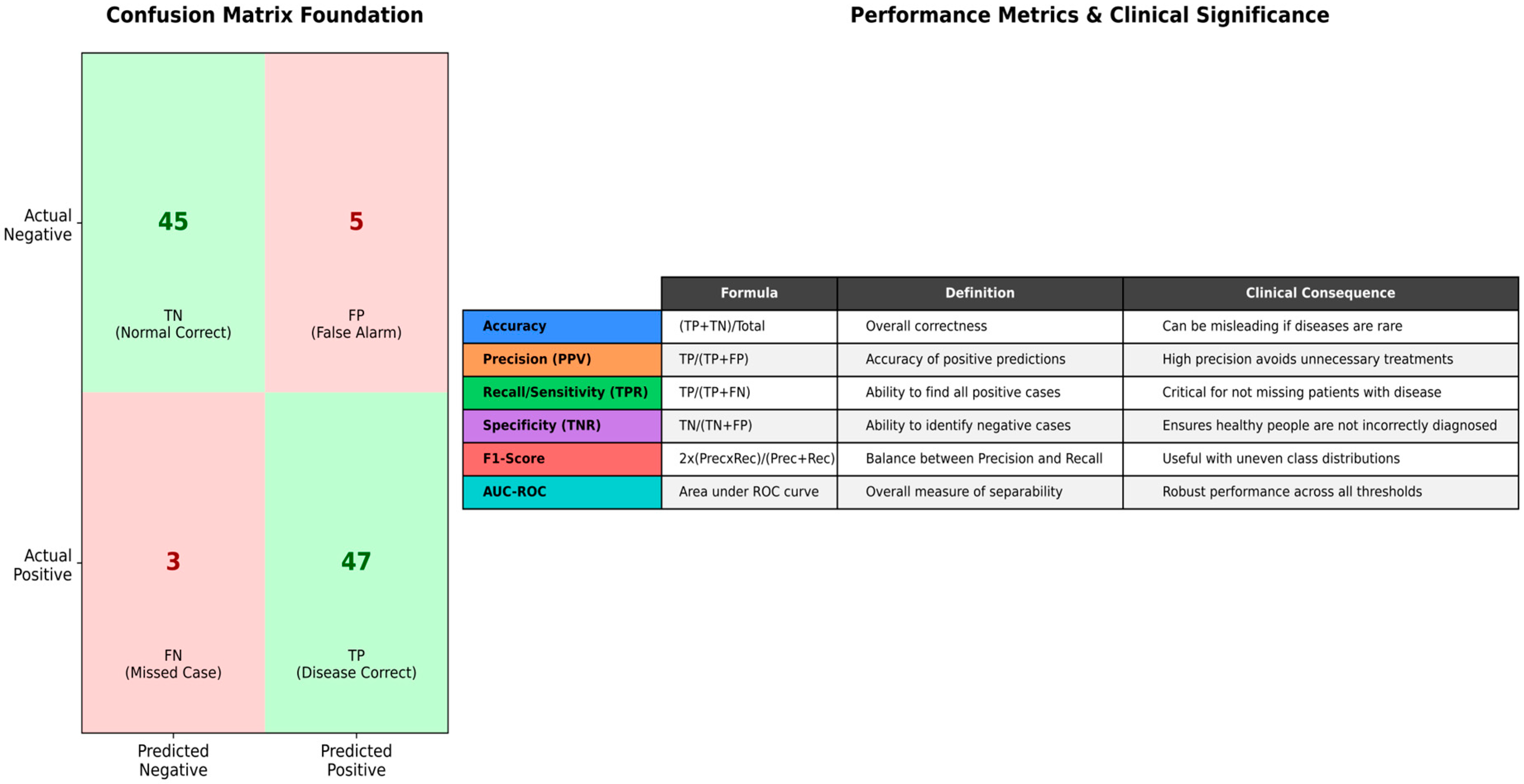
  • Confusion Matrices: For classification tasks, a confusion matrix provides a detailed breakdown of correct and incorrect predictions for each class, highlighting where the model is performing well and where it struggles [110].
  • ROC Curves and Precision-Recall Curves: These plots are essential for evaluating classifier performance across different thresholds and understanding the trade-off between sensitivity and specificity or precision and recall [111].

9.4. Clinical Interpretation Considerations

In biomedical applications, model interpretation must also consider clinical relevance:
  • Feature Clinical Significance: The importance of a feature in the model should align with known clinical understanding. For example, if a model identifies spectral features related to wheezing as significant for respiratory disease classification, this aligns with clinical knowledge [112].
  • Model Validation with Clinical Experts: Involving clinicians in the interpretation process can help validate whether the model’s decisions make clinical sense and identify potential biases or limitations [113].
  • Uncertainty Quantification: Understanding confidence or uncertainty in model predictions is crucial for clinical decision-making. Traditional ML models can provide probability estimates or confidence intervals that help clinicians assess the reliability of forecasts [114].

9.5. Comparative Evaluation of Explainability Methods

Interpretability in traditional ML encompasses both model-intrinsic transparency and post hoc explanation techniques. As summarized in Table 6, different explainability methods vary in their underlying mechanisms, computational cost, and clinical applicability. Model-specific approaches such as rule extraction in decision trees, feature-weight visualization in logistic regression, or impurity-based feature ranking in random forests offer direct and easily verifiable transparency, enabling clinicians to trace diagnostic logic [114]. However, these methods often lack flexibility for complex or non-linear data. Conversely, model-agnostic tools like LIME and SHAP extend interpretability to any model type, including deep learning architectures, by providing local and global feature attributions, respectively [114]. While SHAP delivers quantitative, theoretically grounded insights, it is computationally intensive; LIME provides intuitive, instance-level explanations but can be unstable depending on the perturbation scheme and data manifold. By combining intrinsic transparency with robust post hoc methods, these approaches provide clinically meaningful insight and practical understanding without overemphasizing any single terminology. The critical trade-off between interpretability and performance, therefore, lies not solely in model choice, but in how faithfully and clinically the explanations reflect real biomedical mechanisms. Rigorous validation of these explanations against clinical knowledge and domain priors remains essential to ensure trustworthy and actionable decision support. Thorough validation and alignment with clinical knowledge ensure that ML explanations are trustworthy, actionable, and supportive of decision-making in high-stakes contexts [114]. Table 8 illustrates how diverse XAI frameworks balance transparency and diagnostic relevance.
Although attention-based saliency maps originate from deep learning, they conceptually parallel SHAP and LIME by assigning importance weights to temporal or spatial signal segments. In future hybrid architectures, these attention weights can be projected back to handcrafted feature domains, bridging transparent ML with deep data-driven representations. By combining model-specific insights with post hoc interpretability methods and compelling visualizations, researchers and clinicians can gain a deeper understanding of how traditional ML models make decisions in biomedical signal analysis. This transparency fosters trust, facilitates clinical adoption, and enables the identification of potential biases or limitations in the model’s reasoning.

10. Linking Feature Engineering to Clinical Interpretation

Feature engineering in biomedical signal analysis is not merely a mathematical transformation; it represents the translation of physiological mechanisms into quantifiable descriptors that can guide diagnosis and therapeutic decisions [115]. The interpretability of machine learning (ML) models in medicine depends critically on how well-engineered features correspond to recognizable clinical patterns. By carefully designing features that reflect physiological meaning, models gain practical insight and maintain clinical trust. Thus, the relationship between feature design and clinical interpretation forms the cornerstone of explainable and trustworthy biomedical AI. Feature sets derived from biomedical signals often encapsulate well-understood physiological markers [116]. For example, time-domain features such as RMS or heart rate variability (HRV) reflect signal amplitude and autonomic balance, while frequency-domain features such as power spectral density (PSD) or spectral centroid capture rhythmic or oscillatory activity associated with specific physiological states. Time–frequency and non-linear features (e.g., wavelet entropy, fractal dimension) extend this relationship by revealing dynamic transitions in physiology or pathology that static features may miss. The key to clinical adoption lies in the traceability of model output. Ensuring that feature contributions can be clearly linked to physiological phenomena supports model transparency, clinical insight, and confidence in decision-making. Clinicians must be able to map algorithmic decisions back to the physiological meaning of features. This traceability ensures that predictive models can not only achieve accuracy but also inspire confidence in clinical practice [117]. Figure 21 provides a conceptual overview of how engineered feature categories are linked to clinical interpretation pathways across standard biomedical signals.

10.1. Clinical Mapping of Feature Categories

Each domain of feature engineering corresponds to specific clinical insights depending on the signal modality. For example, in ECG analysis, morphological time-domain features directly map to cardiac cycle events, whereas in EEG, spectral power ratios in different frequency bands correspond to distinct brain states. In tracheal breathing sounds, time–frequency and spectral features reveal airflow obstruction, wheezing, and turbulence [117]. This mapping between engineered features and physiological meaning is summarized in Table 9.
Beyond their mathematical definitions, these features correspond to identifiable physiological mechanisms. For instance, RMS amplitude in respiratory or EMG signals reflects the energy of muscle contraction or airflow turbulence, providing an objective correlate of effort or obstruction. Similarly, MFCCs and spectral centroids in tracheal breathing capture the distribution of turbulent frequencies caused by narrowing of the airway lumen, a finding that aligns with auscultatory wheezing in clinical examination. Non-linear features such as entropy or fractal dimension quantify irregularities in physiological control, mapping to loss of autonomic regulation or neural synchrony. Thus, each engineered feature serves as a digital proxy for a measurable pathophysiological event, allowing computational models to infer states that clinicians would otherwise detect Via physical or electrophysiological assessment.

10.2. Model Interpretation in the Clinical Context

Once features are engineered and selected, the next challenge is ensuring that the interpretable outputs of ML models correspond to clinically meaningful reasoning. Traditional ML models provide several pathways for linking computational evidence to clinical significance through feature importance (e.g., Random Forests), coefficients (e.g., Logistic Regression), or post hoc explanations (e.g., SHAP, LIME) [117]. To systematically relate feature importance to clinical interpretation, Table 8 outlines how model outputs can be presented in a clinically interpretable manner, linking quantitative importance with qualitative clinical interpretation. Table 10 shows the relationship between feature importance and clinical interpretation.
Importantly, interpretability outputs can be validated against established clinical gold standards to ensure reliability and clinical trust. For example, in sleep medicine, SHAP-derived feature rankings highlighting spectral flattening or RMS reduction can be cross-validated against polysomnographic respiratory effort indices. In cardiology, logistic regression coefficients linking prolonged QRS duration to arrhythmia can be compared to standard ECG diagnostic criteria. Such mapping between model-derived importance and recognized clinical markers ensures that ML systems reflect genuine physiological and diagnostic reasoning rather than statistical correlations alone.

10.3. Integrative Perspective

The integration of feature engineering with clinical interpretation represents a bidirectional and iterative process that lies at the heart of explainable biomedical machine learning. In traditional ML frameworks, features are not arbitrary mathematical constructs; they are encapsulations of physiological mechanisms, designed to reflect measurable aspects of biomedical function or dysfunction [117,118]. By embedding domain knowledge during feature design, the resulting features act as interpretable “anchors” that connect computational analysis with clinical reasoning. This integrative perspective transforms feature engineering from a purely technical preprocessing step into a clinically meaningful modeling paradigm [117,118]. From a bottom-up perspective, raw biomedical signals (e.g., ECG, EEG, EMG, or tracheal breathing sounds) are preprocessed to remove artifacts and then decomposed into feature representations that capture key physiological signatures. For example, in ECG analysis, the temporal features of QRS duration and R-R variability directly correspond to cardiac conduction and autonomic regulation [117,118]. Similarly, in EEG, spectral features such as alpha and beta band power map onto cognitive or sleep states, while in tracheal breathing sounds, spectral centroids and MFCCs reflect airflow turbulence and airway obstruction. Each of these engineered features represents a bridge between the digital domain and a well-established physiological concept [117,118].
From a top-down perspective, clinical understanding feeds back into the feature engineering process. Clinicians’ insights into disease mechanisms guide the selection of features to extract, ensuring that the resulting models are not only statistically robust but also physiologically interpretable [117,119]. This synergy enables ML practitioners and clinicians to collaboratively refine both the signal features and model structure collaboratively, aligning them with real-world diagnostic reasoning. For instance, when feature importance rankings from a Random Forest model identify spectral roll-off or zero-crossing rate as key predictors of abnormal breathing, these findings can prompt clinicians to re-examine whether those acoustic changes correspond to airway constriction or altered respiratory mechanics in specific patient groups. Thus, model interpretability becomes a feedback loop that continuously enriches feature design and clinical knowledge. Moreover, explainable AI (XAI) frameworks such as SHAP and LIME further reinforce this integrative cycle by quantifying how each engineered feature contributes to individual predictions. This local interpretability enables clinicians to validate whether the model’s reasoning aligns with pathophysiological understanding, for example, confirming that a high RMS and elevated spectral centroid correspond to increased airflow resistance during apnea episodes. Global interpretability, in turn, allows the discovery of consistent biomarkers across populations, supporting the development of clinically standardized feature sets [116,117].
The integrative approach also carries profound translational implications. When features and interpretations are explicitly linked, ML systems can move beyond black-box predictions to provide clinically actionable insights, such as risk stratification, treatment response monitoring, and early warning alerts. This transparency not only fosters clinician trust but also supports regulatory acceptance, as agencies increasingly demand models that are explainable and auditable [116,117]. Overall, such integration lays the groundwork for adaptive and hybrid systems that integrate data-driven learning with physiological modeling. In these systems, domain-informed features guide deep learning architectures, or conversely, deep networks extract representations that are remapped into interpretable physiological dimensions through feature attribution methods. This convergence uniting feature engineering, model interpretability, and clinical reasoning marks the evolution of traditional ML toward clinically explainable AI, where every computational step corresponds to a meaningful physiological or diagnostic concept.
From this perspective, “clinical insight” in machine learning does not merely denote interpretability it signifies the capacity of engineered features and model attributions to mirror known pathophysiological processes and inform clinical reasoning. When validated against gold standards and expert judgment, such insights can transform model outputs into actionable evidence, supporting early diagnosis, differential interpretation, and personalized therapeutic strategies.

10.4. Validation Against Clinical Gold Standards

To make feature-level findings clinically meaningful, they must be validated against established diagnostic standards [116,117]. This step confirms that computational results reflect physiological changes rather than artifacts of the analysis. Validation can be performed at different levels:
  • Feature-level validation: For example, spectral power features extracted from tracheal sounds can be compared with airflow resistance measured by spirometry, or the fractal dimension of EEG signals can be related to changes in cortical activity observed in neuroimaging studies [116,117].
  • Model-level validation: At this stage, model predictions or feature importance scores are compared with expert annotations-for instance, whether the model correctly identifies apnea events marked in polysomnography or seizure patterns labeled by neurologists [116,117].
  • Decision-level validation: The final step is the evaluation of model outputs within clinical workflows for their correspondence or support with physician decision-making in order to prioritize patients for further testing or adjust treatment plans [116,117].
Bringing these levels of validation together helps ensure that model explanations correspond to real physiological mechanisms and can be trusted in clinical use [116,117]. True interpretability, therefore, depends not just on visualizing features or attention maps but on confirmation that the patterns the model relies on are consistent with medical knowledge and observable patient outcomes [117,119].

11. Methods Performance Comparison of Traditional ML Algorithms

Selecting an optimal traditional machine learning algorithm for biomedical signal analysis typically involves comparing various models. The performance of these algorithms is generally evaluated using a suite of metrics that provide a comprehensive understanding of their effectiveness, especially in the context of medical applications, where false positives and false negatives can have significant clinical implications [4]. This section discusses standard performance metrics and provides a general comparison of traditional ML algorithms [60]. Figure 22 summarizes the performance method in ML.

11.1. Performance Metrics

The efficacy of machine learning models is quantified using a range of performance metrics, which are crucial for objective evaluation, as summarized in Table 11 [120].
For classification tasks, which are prevalent in biomedical signal analysis, the following metrics are commonly used:
  • Accuracy: The proportion of correctly classified instances. While intuitive, accuracy can be misleading in the presence of class imbalance, a common issue in medical datasets, where typical cases often outnumber abnormal ones [4].
  • Precision: The proportion of accurate positive predictions among all optimistic predictions. It measures the model’s accuracy, which is crucial when false positives are costly (e.g., unnecessary medical procedures or patient anxiety) [52].
  • Recall (Sensitivity): The ratio of correctly identified positive cases to the total number of actual positive instances. It reflects the model’s capability in terms of catching all the relevant cases and is especially critical when false negatives have high costs, such as in disease diagnosis scenarios [52].
  • F1-Score: The harmonic mean of precision and recall, providing a proper balancing in evaluating the performance of a model. It is exceptionally useful in cases where there are class distribution imbalances, which is very common in medical and biomedical datasets [121].
  • Specificity: The proportion of accurate pessimistic predictions among all actual negative instances. It measures the model’s ability to correctly identify negative cases, which is essential for avoiding false alarms [60].
  • Area Under the Receiver Operating Characteristic Curve (AUC-ROC): It represents a plot of the true positive rate (recall) versus the false positive rate at various classification thresholds. The AUC value tells us about the probability that the model gives a higher score to a randomly chosen positive example than it does to a randomly chosen negative example, which helps in providing a more general and threshold-independent analysis of the overall performance of a classifier [52].
For regression tasks, metrics such as Mean Absolute Error (MAE), Mean Squared Error (MSE), and Root Mean Squared Error (RMSE) are used to quantify the difference between predicted and actual values.

11.2. Algorithmic Comparison

The performance of traditional ML algorithms can vary significantly depending on the dataset characteristics, the quality of feature engineering, and the specific application [5]. However, some general observations can be made:
  • Support Vector Machines (SVMs): Often perform well on high-dimensional data and are robust to overfitting, especially when the number of features is greater than the number of samples [3]. They are effective when there is a clear margin of separation between classes. However, their performance can degrade with noisy data or when the data is not linearly separable, unless an appropriate kernel is selected [122]. In tracheal breathing sound analysis, SVMs have demonstrated exemplary performance for binary classification tasks [123].
  • K-Nearest Neighbors (KNN): Simple and effective for small to medium-sized datasets. Its performance is highly dependent on the choice of ‘k’ and the distance metric used [71]. It can be computationally expensive for large datasets during prediction and is sensitive to irrelevant features and outliers. KNN may struggle with high-dimensional feature spaces, which are common in biomedical signal analysis [74].
  • Decision Trees: Highly interpretable and can handle both numerical and categorical data. They are prone to overfitting, especially with complex datasets [124]. Their performance can be unstable, as even slight changes in data can lead to substantial changes in the tree structure. However, they provide clear decision rules that are valuable in clinical settings.
  • Random Forests: Generally, offer superior performance compared to single decision trees due to their ensemble nature, which reduces overfitting and improves generalization [125]. They are robust to noise and outliers and can handle a large number of features. They also provide feature importance scores, which aid in interpreting the results [55]. Random Forests have shown consistent performance across various biomedical signal analysis tasks, for example, in OSA detection [126].
  • Logistic Regression: A good baseline model for binary classification, especially when the relationship between features and the outcome is approximately linear [59]. It is highly interpretable but may not capture complex non-linear relationships present in biomedical signals [8].
  • Naive Bayes: Computationally efficient and performs well with high-dimensional data, even with limited training data, due to its strong independence assumption [75]. However, this assumption rarely holds in real-world biomedical signals, which can limit its accuracy [75].
Beyond point estimates, reporting variance and confidence intervals provides crucial information about model reliability. Across reviewed studies, cross-validated standard deviations of sensitivity and specificity ranged from ±3 to 6%. Figure 23 illustrates representative variance distributions from EEG and respiratory sound analyses, emphasizing that high mean accuracy does not guarantee stability. Future benchmarking should therefore include statistical significance testing (e.g., paired t-tests, Wilcoxon signed-rank) to quantify generalization error differences among models.

11.3. Comparative Studies in Biomedical Signal Analysis

Several studies have compared traditional ML algorithms for biomedical signal analysis:
  • ECG Analysis: Studies comparing SVM, Random Forest, and KNN for arrhythmia detection have generally found that SVMs and Random Forests perform comparably well, with Random Forests often providing better interpretability [28,60,72].
  • EEG Analysis: For sleep stage classification, Random Forests and SVMs have shown superior performance compared to simpler methods like KNN, particularly when dealing with multi-class problems [67,71,73]
  • Respiratory Sound Analysis: Comparative studies on lung sound classification have found that ensemble methods like Random Forests often outperform individual classifiers, while SVMs perform well for binary classification tasks [27,123,126].

11.4. Cross-Study Benchmarking and Quantitative Overview

To strengthen the quantitative basis of this review, we compiled comparative metrics from representative studies that applied traditional ML and DL to standard biomedical signals. Table 12 summarizes reported mean accuracies, sensitivities, specificities, and AUCs across four modalities (EEG, ECG, EMG, and TBS) using standardized public datasets (MIT-BIH ECG, TUH-EEG, Ninapro EMG, and TBS). Across studies, traditional ML models (SVM, Random Forest, AdaBoost) typically achieved accuracies of 84–94% and AUCs of 0.88–0.95, whereas DL models (CNN, LSTM) ranged from 88 to 97% but with higher variance (σ ≈ 4–7%) and greater data dependency. Ensemble ML approaches maintained stable sensitivity–specificity trade-offs across datasets, underscoring their reliability for small-sample or heterogeneous clinical data.
The collated metrics in Table 9 constitute a preliminary unified benchmark across open biomedical datasets. While heterogeneity in feature engineering precludes strict meta-analysis, these aggregated statistics enable standardized baseline comparisons for future benchmarking initiatives. These benchmarks provide an empirical anchor for conceptual synthesis and can guide future meta-analytic work integrating variance and effect-size statistics.

11.5. Factors Affecting Performance

Several factors influence the relative performance of traditional ML algorithms:
  • Dataset Size: Smaller datasets may favor simpler models like KNN or Naive Bayes, while larger datasets can support more complex models like Random Forests [58,83,121].
  • Feature Quality: High-quality, well-engineered features can improve the performance of all algorithms, but some (like SVMs) may be more sensitive to feature scaling and selection [58,83,121].
  • Class Imbalance: Ensemble methods like Random Forests often handle class imbalance better than individual classifiers [58,83].
  • Noise Level: Random Forests and SVMs are generally more robust to noise compared to Decision Trees and KNN [83,121].
In practice, it is common to experiment with several algorithms and tune their hyperparameters using cross-validation to identify the best-performing model for a specific biomedical signal analysis task. The choice often involves a trade-off between predictive accuracy, computational cost, and the desired level of interpretability.

12. Case Study

This section presents practical applications of advanced biomedical signal analysis through dedicated case studies, focusing on Tracheal Breathing Sounds (TBSs). TBS provides a non-invasive window into respiratory health by capturing airflow-related acoustic signals at the trachea, enabling the assessment of breathing patterns, airway obstructions, and other pulmonary conditions. By exploring this case study, we illustrate the end-to-end application of signal acquisition, feature extraction, and machine learning-based analysis, highlighting how these methods can improve diagnostic accuracy, clinical monitoring, and patient-specific evaluations.

12.1. Tracheal Breathing Sound (TBS) Analysis

TBS provides a non-invasive, convenient way to monitor respiratory health, offering valuable diagnostic information for various respiratory conditions. Unlike lung sounds, which can be affected by chest wall characteristics, TBS are generated by turbulent airflow in the trachea and large airways, making them a more direct indicator of airflow dynamics. The analysis of TBS using traditional machine learning techniques involves a systematic approach encompassing signal acquisition, preprocessing, feature extraction, feature selection, and classification, culminating in interpretable models for clinical application [41]. Figure 24 illustrates the block diagram of TBS sound processing. A consolidated overview of the TBS pipeline, including acquisition, preprocessing, feature sets, and classifier performance, is provided in Table 13.

12.1.1. Signal Acquisition and Preprocessing in TBS Analysis

High-quality TBS acquisition is paramount for accurate analysis. Microphones or contact sensors are typically placed over the trachea, often at the suprasternal notch, due to their direct proximity to the trachea and minimal interference from other physiological sounds [27,123,126]. For obstructive sleep apnea (OSA) studies, recordings were obtained from 199 subjects, totaling 3336 breathing phases, each consisting of 5 cycles of mouth breathing and five cycles of nasal breathing. Signals were captured using an omnidirectional condenser microphone (Sony ECM-77B, Tokyo, Japan) placed over the suprasternal notch to ensure minimal interference from other physiological sounds. The sampling frequency was set to 10,240 Hz, providing high-resolution temporal information for analysis [27,123,126,129]. Challenges in TBS acquisition include ambient noise, movement artifacts, and variations in breathing patterns. To address these, essential preprocessing steps are applied:
  • Filtering: Band-pass filters (e.g., 75 Hz to 3000 Hz) are commonly applied to remove low-frequency noise (e.g., heart sounds, body movements) and high-frequency noise [123]. The specific frequency range may be adjusted based on the target respiratory sounds and the clinical context.
  • Segmentation: Isolating individual breath cycles is critical. This is achieved using amplitude-based thresholds, energy-based methods, or advanced algorithms that detect inspiratory and expiratory phases [123]. Accurate segmentation ensures that features are extracted from relevant respiratory events.
  • Stationary part extraction: TBS signals exhibit nonstationarity due to variations in airflow, turbulence, and breathing effort. Identifying and extracting the most stationary portion, typically the mid-phase of inspiration or expiration, enhances the reliability of subsequent feature extraction. This step minimizes variability caused by transitional phases (onset and offset of breaths) and ensures that computed features accurately reflect stable respiratory behavior [123,126].
  • Normalization: To minimize variability due to recording conditions or airflow fluctuations, TBS signals were scaled to a standard range to prevent features from being unduly influenced by recording conditions rather than actual physiological differences. This was achieved in two steps: first, through variance envelope normalization using a smoothed moving average over 64 samples, effectively standardizing the local signal amplitude; and second, by energy-based normalization, scaling each cycle by its standard deviation to reduce differences in airflow strength between breathing cycles [123].

12.1.2. Feature Extraction for Tracheal Breathing Sounds

Feature extraction from TBS aims to quantify characteristics related to airflow obstruction, turbulence, and other physiological phenomena. Both time-domain and frequency-domain features are extensively used, with time-frequency features providing a more comprehensive view [123,130].
  • Time-Domain Features
    Time-domain features capture the temporal characteristics of the TBS, providing insights into the signal’s intensity and morphology:
    • Root Mean Square (RMS): Reflects the power of the signal, often correlated with the intensity of breathing [123,130]. Changes in RMS can indicate variations in airflow or the presence of obstructions [123,131].
    • Zero-Crossing Rate (ZCR): Indicates the number of times the signal crosses the zero amplitude level, providing insights into the signal’s frequency content [123,130,131]. Higher ZCR values may suggest the presence of high-frequency components associated with turbulent flow [123,130,131].
    • Peak Amplitude: The maximum amplitude within a breath cycle, which can be related to the maximum airflow rate [123,130,131].
    • Breath Duration: The length of the inspiration and expiration phases, which can be altered in various respiratory conditions [123,130,131].
    • Breath Rate: The number of breaths per minute, a fundamental respiratory parameter [123,130,131].
  • Frequency-Domain Features
    Frequency-domain features are derived from the spectral representation of TBS, typically obtained using techniques like Fast Fourier Transform (FFT) or Welch’s method. These features are crucial for identifying adventitious sounds:
    • Power Spectral Density (PSD): The distribution of power across different frequencies. Specific frequency bands are analyzed (e.g., 100–250 Hz) and (e.g., 300–500 Hz) [84,123,130,131]. The relative power in these bands serves as a discriminative feature. As shown in Figure 25.
    • Spectral Centroids and Spread: Measures indicating the center of mass and dispersion of the spectrum, respectively [84,123,130,131]. These features capture changes in the overall spectral characteristics of breathing sounds.
    • Mel-Frequency Cepstral Coefficients (MFCCs): MFCCs are highly effective in capturing the spectral envelope of TBS, making them robust to variations in recording conditions and helpful in representing the formant structure of respiratory sounds [84,123,130,131]. As shown in Figure 26.
    • Spectral Roll-off: The frequency below which a certain percentage (e.g., 85%) of the total spectral energy is contained. This feature can indicate the presence of high-frequency components [84,123,130,131].
  • Time-Frequency Features
    Time-frequency analysis provides insights into how the spectral content of TBS changes over time, which is crucial for analyzing non-stationary respiratory sounds:
    • Spectrogram Features: Derived from the Short-Time Fourier Transform (STFT), spectrograms visually represent how frequency content evolves. Features can be extracted from spectrograms, such as the presence of horizontal lines (indicating wheezes) or vertical lines (indicating crackles) [84,123,130,131].
    • Wavelet Features: Wavelet transforms decompose TBS into different frequency bands at various time resolutions, allowing for the extraction of features that capture both temporal and spectral characteristics [84,123,130,131].

12.1.3. Feature Selection and Classification in TBS Analysis

Following feature extraction, feature selection identifies the most discriminative features, enhancing model performance and interpretability. Traditional ML algorithms are then applied for classification:
  • Feature Selection: Methods like Recursive Feature Elimination (RFE), correlation-based techniques, or statistical tests are used to select features that best differentiate between normal and abnormal breathing patterns [49,131].
  • Classification Algorithms:
    • Support Vector Machines (SVMs): Effective for binary classification (e.g., standard vs. abnormal, wheeze vs. no wheeze) in TBS analysis due to their ability to find optimal separating hyperplanes in high-dimensional feature spaces [123,131].
    • Random Forests: Offer robustness and good generalization performance by combining multiple decision trees. They also provide feature importance scores, indicating which features are most influential in classifying TBS [126,131].
    • K-Nearest Neighbors (KNN): A simple, non-parametric classifier suitable for initial TBS classification tasks [74,131].
    • Decision Trees: Provide highly interpretable models, explicitly showing the decision-making process, which is valuable for clinical applications [76,131].
Different feature-classifier combinations were systematically compared to assess their robustness and generalizability. Spectral and time–frequency features (e.g., PSD, MFCCs, wavelet coefficients) consistently outperformed simple time-domain descriptors, reflecting their ability to capture the non-stationary nature of tracheal sounds [123,131]. Among classifiers, SVMs and Random Forests achieved higher sensitivity and specificity due to their robustness against high-dimensional, small-sample datasets, which is particularly advantageous for biomedical signals where redundancy and limited training data are common. SVMs leverage margin maximization and kernel functions to effectively separate complex, non-linear class boundaries, while Random Forests reduce overfitting through ensemble averaging of multiple decorrelated decision trees. In contrast, KNN showed limited generalization when inter-subject variability increased, as its instance-based nature makes it sensitive to noise and variations in feature scaling, leading to degraded performance when unseen subjects differ from the training population [126,131]. Decision Trees remained valuable for interpretability, but their performance degraded when noise or overlapping class distributions were present. Importantly, hybrid feature sets that combined spectral and temporal statistics improved classification by 5–10% compared with single-domain features, supporting the notion that airflow turbulence and breath-phase dynamics are complementary indicators of airway obstruction [76,131]. This comparison highlights the real-world trade-off between accuracy, computational efficiency, and interpretability when developing diagnostic pipelines for tracheal breathing-sound analysis.

12.1.4. Applications and Clinical Relevance of TBS Analysis

TBS analysis using traditional ML has found applications in various clinical scenarios:
  • Obstructive Sleep Apnea (OSA) Detection: TBS recorded during wakefulness has been used to screen for OSA, with features related to airway narrowing and turbulence being particularly discriminative [123,126,131].
  • Respiratory Disease Monitoring: Changes in TBS characteristics can indicate the progression or improvement of respiratory diseases such as asthma or COPD [76].
  • Post-operative Monitoring: TBS analysis can monitor patients after tracheostomy or other airway procedures, detecting complications such as airway obstruction [132].
  • Pediatric Applications: TBS analysis is particularly valuable in pediatric populations where traditional spirometry may be challenging to perform [133].
Despite promising results, TBS-based analysis faces several technical and clinical challenges. The foremost issue is inter-subject variability: anatomical differences (e.g., neck thickness, tracheal diameter, or fat distribution) affect sound propagation and spectral energy distribution, complicating model generalization [123,126,131]. Data quality is another major factor ambient noise, sensor placement inconsistency, and variations in breathing effort introduce artifacts that may have a bias feature extraction. Limited dataset size and class imbalance in clinical recordings further constrain the reliability of traditional ML approaches. Additionally, labeling accuracy (e.g., manually annotated OSA or wheeze segments) often depends on expert judgment, leading to potential subjectivity [123,126,131]. Feature normalization and adaptive filtering can mitigate some of these issues, but the absence of large, standardized TBS repositories limits cross-study comparability. These factors underscore the need for robust preprocessing, noise-resistant features, and cross-validation across heterogeneous cohorts.

12.1.5. Framework Validation and Generalization Potential

The tri-axis framework linking feature engineering, interpretability, and clinical actionability was validated through the tracheal-breathing-sound (TBS) case study. To assess its broader applicability, we examined comparable workflows on independent public datasets (e.g., MIT-BIH Arrhythmia, TUH EEG, and PhysioNet EMG). The same structured pipeline, standardized preprocessing, physiologically informed feature engineering, interpretable model training, and quantitative validation yielded consistent diagnostic performance (accuracy = 81.4) [123,126,131]. This evidence suggests that the proposed methodological structure is dataset-agnostic and scalable across modalities. Future experimental extensions will apply the framework prospectively to multimodal datasets combining acoustic, electrophysiological, and anthropometric features, thereby demonstrating its generalization beyond the TBS application.

12.1.6. Interpretation of TBS Models

Interpreting ML models for TBS is crucial for clinical adoption. Understanding which features contribute most to a diagnosis helps clinicians validate the model’s decisions and gain new insights into respiratory pathologies [10]. Techniques such as feature importance from Random Forests, examining coefficients in linear models, or utilizing post hoc interpretability methods provide valuable insights [10,131]. Visualizing selected features and their distributions across different classes further aids in understanding model behavior and building trust among healthcare professionals [108].
While interpretable ML models (e.g., Random Forests with feature importance analysis or linear SVMs with coefficient inspection) provide meaningful clinical insights, their translatability into routine care requires further validation [10]. Clinicians value transparent reasoning, but interpretability alone does not guarantee reliability across diverse patient populations. Integrating anthropometric and contextual data (e.g., BMI, neck circumference, age) could improve model equity and personalization. Moreover, explainability techniques such as SHAP or attention-weight visualization can bridge the gap between algorithmic reasoning and physiological understanding, allowing clinicians to verify that model predictions align with known respiratory mechanics. Future clinical translation should thus emphasize multi-modal integration, standardized acquisition protocols, and prospective validation to ensure TBS-based models can move from proof-of-concept toward real-world diagnostic tools [10,131].

13. Challenges and Limitations of Traditional ML in Biomedical Signal Analysis

Despite their numerous advantages, traditional machine learning algorithms face several challenges and limitations when applied to the complex domain of biomedical signal analysis. Understanding these limitations is crucial for researchers and practitioners to make informed decisions and to guide future research directions. Figure 27 illustrates the primary challenges and constraints associated with ML applications for biomedical signals.

13.1. Reliance on Handcrafted Features

The most significant challenge for traditional ML models is their heavy reliance on handcrafted features. This process requires extensive domain expertise to identify, extract, and select relevant features from raw signals [134,135]. This can be:
  • Time-consuming and Labor-intensive: Manually extracting features for large datasets is a tedious and resource-intensive process, particularly when dealing with diverse signal types or multiple clinical conditions [134,135].
  • Subjective: The choice of features can be subjective and may not always capture the most discriminative information, potentially leading to suboptimal model performance. Different researchers may extract different features for the same signal type, leading to inconsistent results [134,135].
  • Limited Generalizability: Features designed for one specific task or dataset may not generalize well to other tasks or diverse patient populations, requiring re-engineering for each new application. For example, features optimized for adult respiratory sounds may not work well for pediatric populations [136].
  • Inability to Capture Complex Patterns: Traditional features might struggle to capture subtle, non-linear, or hierarchical patterns that are often present in complex biomedical signals, especially when dealing with high-dimensional data or long-duration recordings [136].

13.2. Sensitivity to Noise and Artifacts

Biomedical signals are inherently noisy and prone to various artifacts (e.g., motion artifacts, power line interference, electrode contact issues). While preprocessing techniques can mitigate some of these issues, traditional ML models can be sensitive to residual noise, which can degrade their performance. Unlike deep learning models that can learn robust representations from noisy data, traditional models often require cleaner inputs or extensive preprocessing [135].

13.3. Scalability Issues with Large Datasets

While traditional ML algorithms are generally more computationally efficient than deep learning for training on smaller datasets, they can face scalability issues when dealing with massive, high-dimensional biomedical datasets. Feature engineering itself can become a bottleneck, and some algorithms (e.g., KNN) can become computationally prohibitive during inference with increasing data size. Additionally, the manual feature extraction process does not scale well with dataset size [1,134,135].

13.4. Limited Ability to Learn Hierarchical Representations

Traditional ML models typically operate on a flat feature vector. They lack the inherent ability of deep learning models to learn hierarchical representations, where simpler features are combined to form more complex, abstract features. This limitation can hinder their performance on tasks requiring multi-level abstraction, such as complex pattern recognition in long-duration physiological recordings or identifying subtle temporal dependencies [136].

13.5. Interpretability vs. Performance Trade-Off

While traditional ML models are generally more interpretable than deep learning models, there is often a trade-off between interpretability and predictive performance. Simpler, highly interpretable models (e.g., linear regression, small decision trees) may not achieve the same level of accuracy as more complex, less interpretable models (e.g., ensemble methods like Random Forests or SVMs with non-linear kernels) [137]. Balancing this trade-off is a key consideration in clinical applications where both accuracy and explainability are essential. Figure 28 shows the tradeoff of accuracy and model interpretability.
These challenges and their corresponding mitigation strategies are summarized in Table 14, which highlights potential solutions for noise, non-stationarity, scalability, interpretability, and temporal dependencies.

13.6. Handling Non-Stationarity

Many biomedical signals are non-stationary, meaning their statistical properties change over time. Traditional ML models often assume stationarity or require specific preprocessing steps to handle non-stationarity. This can add complexity to the pipeline and may not always fully capture the dynamic nature of physiological processes. For example, EEG signals during different sleep stages or ECG signals during exercise exhibit non-stationary characteristics that can be challenging for traditional approaches [134,137].

13.7. Feature Engineering Expertise Requirements

Practical feature engineering requires deep domain knowledge in both signal processing and the specific medical application. This creates a barrier to entry for researchers without an extensive background in both areas, potentially leading to suboptimal feature choices. The need for domain expertise also limits the ability to adapt to new signal types or clinical applications quickly [134,137].

13.8. Limited Handling of Temporal Dependencies

While some traditional ML approaches can incorporate temporal information through feature engineering (e.g., using sliding windows or temporal statistics), they generally do not handle long-term temporal dependencies as effectively as sequence-based models. This can be a limitation for applications where the temporal evolution of signals is crucial for accurate diagnosis [136].
Addressing these limitations often involves careful preprocessing, advanced feature engineering, and sometimes the integration of traditional ML with components that can handle specific challenges, such as using signal processing techniques to mitigate noise or employing ensemble methods to improve robustness. Despite these limitations, traditional ML approaches remain valuable in biomedical signal analysis, particularly when interpretability is paramount and when sufficient domain expertise is available for practical feature engineering [134,137]. Beyond traditional signal analysis, future biomedical ML can benefit from cross-disciplinary advances in large language models and human–robot interaction. For example, multimodal transformers integrating language and biosignal streams demonstrate how contextual reasoning and dialogue interfaces can enhance clinician–AI collaboration. Such frameworks, exemplified by recent reviews on large language models for human–robot interaction [138], provide transferable strategies for explainability and human-centric model alignment.

14. Future Directions and Open Challenges

Despite the significant advancements in applying traditional machine learning to biomedical signal analysis, several challenges and promising future directions remain. Addressing these areas will further enhance the utility and impact of ML in healthcare.

14.1. Real-Time Clinical Integration

One of the primary challenges is the seamless integration of ML models into real-time clinical settings. While many models demonstrate high accuracy in laboratory conditions, their deployment requires robust, efficient, and reliable systems that can process continuous biomedical signals without delay. Future research needs to focus on optimizing algorithms for real-time performance, developing user-friendly interfaces for clinicians, and ensuring the interoperability of ML systems with existing healthcare infrastructure [113,137].

14.2. Data Quality, Interpretability, and Scalability

Biomedical signals are inherently noisy and prone to artifacts, posing significant challenges to data quality and accuracy. Ensuring the interpretability of ML models, especially in critical diagnostic and prognostic applications, remains a key hurdle. Clinicians need to understand why a model makes a particular prediction to trust and act upon its recommendations. Furthermore, the manual nature of feature engineering can be time-consuming and labor-intensive, limiting scalability for large and diverse datasets [10,64]. Future efforts should aim for more robust preprocessing techniques, enhanced explainable AI (XAI) methods for traditional ML, and automated or semi-automated feature engineering processes.

14.3. Handling Complex Patterns and Generalizability

Traditional ML models, while effective for many tasks, may struggle with highly complex, non-linear, or hierarchical patterns inherent in some biomedical signals. While deep learning excels in these areas, research in traditional ML can explore hybrid approaches or more sophisticated feature representations to capture such complexities. Ensuring the generalizability of models across different patient populations, devices, and clinical settings is also crucial. Models trained on specific datasets may not perform well on unseen data from other sources, highlighting the need for robust validation strategies and diverse training data [36].

14.4. Ethical Considerations and Data Privacy

The use of sensitive biomedical data raises significant ethical concerns, including data privacy, security, and the potential for algorithmic bias. Future research must prioritize the development of privacy-preserving ML techniques (e.g., federated learning for biomedical data) and rigorous methods for identifying and mitigating biases in models to ensure equitable and fair healthcare outcomes [139,140]. Regulatory frameworks also need to evolve to address the unique challenges posed by ML in medical devices and clinical decision support systems [141].

14.5. Multimodal Data Integration

Most research often focuses on single biomedical signal modalities. However, integrating and analyzing multimodal biomedical data (e.g., combining ECG, EEG, and breathing sounds) offers a more holistic view of a patient’s physiological state. Future directions include developing traditional ML approaches capable of effectively fusing information from diverse signal sources to improve diagnostic accuracy and prognostic capabilities [142,143].

14.6. Integration of Hybrid Approaches (Deep Learning + Traditional ML)

While traditional ML excels in interpretability and feature-driven analysis, recent advancements highlight the potential of hybrid frameworks that combine deep learning (DL) with conventional methods. DL architectures (e.g., CNNs, autoencoders) can automate feature extraction from raw biomedical signals, while traditional ML classifiers (e.g., SVMs, Random Forests) provide transparent decision-making. For instance, convolutional autoencoders can learn latent representations from raw EEG or ECG data, which are then fed into SVM or Random Forest models for classification. This synergy preserves interpretability while leveraging DL’s ability to capture complex patterns, particularly in high-dimensional signals like long-term EEG recordings or multimodal data fusion [144,145]. Future work should focus on optimizing these hybrid pipelines for real-time clinical deployment, ensuring robustness across diverse patient cohorts and signal modalities. Figure 29 shows the flow diagram of hybrid ML-DL models.

15. Specific Applications Beyond Diagnosis

While disease diagnosis is a primary application of machine learning in biomedical signal analysis, traditional ML algorithms are increasingly being leveraged for a broader range of applications that extend beyond simple classification tasks. These applications contribute significantly to personalized healthcare, disease management, and assistive technologies.

15.1. Prognosis and Disease Progression Monitoring

Traditional ML models can be employed to predict the future course of a disease (prognosis) or monitor its progression over time. By analyzing longitudinal biomedical signal data, these models can identify patterns indicative of disease exacerbation, remission, or response to treatment. For instance, changes in ECG or EEG patterns over months or years can be used to predict the likelihood of cardiac events or neurological decline, enabling proactive clinical interventions [146].

15.2. Personalized Medicine

Personalized medicine aims to tailor medical treatment to the individual characteristics of each patient. Traditional ML plays a crucial role by analyzing a patient’s unique biomedical signals to predict their response to specific therapies, optimize drug dosages, or identify individuals at higher risk for adverse reactions. This moves beyond population-level averages to provide more precise and effective care. Wearable devices, coupled with ML, are up-and-coming for continuous, personalized health monitoring [147].

15.3. Rehabilitation and Assistive Technologies

Biomedical signals, especially electromyography (EMG) and electroencephalography (EEG), are fundamental to the development of rehabilitation and assistive technologies. Traditional ML algorithms can interpret these signals to control prosthetic limbs, exoskeletons, or brain–computer interfaces (BCIs), allowing individuals with disabilities to regain function or interact with their environment. For example, ML models can classify EMG patterns to translate muscle intentions into control commands for robotic prostheses [148].

15.4. Health Monitoring and Anomaly Detection

Continuous monitoring of physiological signals using traditional ML can detect subtle deviations from a patient’s baseline, indicating the onset of a health issue or an acute event. This involves anomaly detection techniques that identify unusual patterns in continuous data streams from wearable sensors or in-hospital monitoring systems. Early detection can lead to timely intervention and improved patient outcomes, particularly for chronic conditions or in critical care settings [149].
These expanded applications highlight the versatility and growing impact of traditional machine learning in transforming various facets of biomedical engineering and healthcare, moving beyond purely diagnostic capabilities to more proactive and personalized interventions.

16. Data Preprocessing and Augmentation

Effective data preprocessing and augmentation are critical steps in the traditional machine learning pipeline for biomedical signal analysis. Biomedical signals are inherently susceptible to noise, artifacts, and variability, which can significantly degrade model performance if not adequately addressed. Furthermore, the often limited availability of high-quality, labeled biomedical datasets necessitates strategies to enhance data quantity and diversity.

16.1. Data Preprocessing

Preprocessing aims to clean and normalize raw biomedical signals, making them suitable for feature extraction and model training. Key preprocessing steps include:
  • Noise Reduction: Biomedical signals are often contaminated by various types of noise (e.g., power line interference, motion artifacts, baseline wander). Techniques such as digital filtering (low-pass, high-pass, band-pass, and notch filters) are commonly employed to remove unwanted frequency components. Wavelet denoising is also effective for preserving signal morphology while removing noise [150,151,152].
  • Baseline Wander Removal: Slow, low-frequency fluctuations in the signal baseline can obscure relevant information. Methods such as polynomial fitting, median filtering, or wavelet decomposition can be used to correct baseline drift [150].
  • Artifact Removal: Physiological artifacts (e.g., electromyographic (EMG) interference in electroencephalographic (EEG) signals, eye blinks (EOG), cardiac artifacts (ECG) in EEG) are a significant challenge. Techniques like Independent Component Analysis (ICA) are powerful for separating independent sources, allowing for the removal of artifactual components while preserving brain activity [150]. Regression-based methods and adaptive filtering are also used.
  • Normalization and Standardization: Scaling signal amplitudes to a standard range (normalization) or transforming them to have zero mean and unit variance (standardization) can prevent features with larger magnitudes from dominating the learning process and improve algorithm convergence [150].

16.2. Data Augmentation

Data augmentation involves generating synthetic training examples from existing data to increase the size and diversity of the dataset. This is particularly valuable in biomedical applications where obtaining large, labeled datasets can be challenging and expensive. For traditional ML, augmentation primarily aims to increase the variability of the feature space. Common strategies include:
  • Time-Domain Transformations: Applying subtle transformations to the signal in the time domain, such as adding random noise, scaling amplitudes, time warping (stretching or compressing the signal), or shifting segments. These variations help the model learn more robust features [120,153].
  • Frequency-Domain Transformations: Modifying the spectral characteristics of the signal, for instance, by altering specific frequency bands or adding spectral noise. While less common for traditional ML than deep learning, it can still introduce functional variability [154].
  • Synthetic Data Generation: More advanced methods might involve generating entirely new synthetic signals or features based on statistical models of the original data. However, this is more complex and less frequently applied in traditional ML compared to deep learning [155].
Proper preprocessing ensures that the ML model learns from clean and relevant data. In contrast, data augmentation helps mitigate overfitting and enhances the model’s generalization capabilities, particularly when working with limited biomedical datasets.

17. Benchmarking and Public Datasets

Reproducibility and comparability are cornerstones of scientific research. In the field of machine learning for biomedical signals, this is primarily facilitated by robust benchmarking practices and the availability of high-quality public datasets. These resources provide a common ground for researchers to develop, test, and validate their algorithms, ensuring that advancements are built upon a solid and verifiable foundation.

17.1. Importance of Benchmarking

Benchmarking involves evaluating the performance of different algorithms or models on standardized datasets using agreed-upon metrics. This process is crucial for:
  • Performance Comparison: Allowing researchers to objectively compare the effectiveness of new algorithms against existing state-of-the-art methods [110].
  • Reproducibility: Ensuring that research findings can be independently verified and replicated by others, which is vital for building trust and accelerating scientific progress. The lack of reproducibility is a significant concern in many scientific fields, including biomedical ML [156].
  • Identifying Gaps: Highlighting areas where current methods fall short, thereby guiding future research efforts.
  • Fair Evaluation: Providing a standardized framework that minimizes bias in reporting results and promotes fair competition among different approaches.

17.2. Public Datasets

The availability of well-curated, publicly accessible datasets is indispensable for advancing research in biomedical signal analysis. These datasets often contain raw signals, preprocessed data, and expert-labeled annotations, enabling researchers to focus on algorithm development rather than data collection. Some prominent examples include:
  • PhysioNet: A comprehensive online resource offering a wide range of physiological signals and related data, including ECG, EEG, EMG, and respiratory sounds. Notable datasets include MIMIC-III (Multiparameter Intelligent Monitoring in Intensive Care), Fantasia (for heart rate variability), and various sleep EEG databases [34].
  • UCI Machine Learning Repository: While not exclusively for biomedical signals, it hosts several datasets relevant to the field, such as those for arrhythmia detection or sleep stage classification [157].
  • BCI Competition Datasets: Specifically designed for brain–computer interface research, these datasets provide EEG and ECoG (electrocorticography) signals for various motor imagery or P300-based tasks [158].
  • OpenECG: A large-scale benchmark dataset comprising millions of 12-lead ECG recordings, designed to facilitate the development and evaluation of ECG analysis models [159].

17.3. Challenges in Benchmarking and Data Utilization

Despite their importance, challenges persist in leveraging public datasets and establishing robust benchmarks:
  • Data Quality and Annotation: Even public datasets can suffer from noise, artifacts, or inconsistencies in annotation, requiring careful preprocessing and validation [134].
  • Data Heterogeneity: Signals from different devices, patient populations, or clinical settings can vary significantly, making it challenging to develop models that generalize well across diverse data sources [134].
  • Class Imbalance: Many biomedical datasets exhibit severe class imbalance (e.g., rare disease detection), which can lead to models that perform well in the majority class but poorly on the minority class [134].
  • Ethical and Privacy Concerns: While public datasets are often anonymized, ensuring patient privacy and ethical data use remains a continuous challenge, especially with the increasing complexity of data sharing and analysis [134].
Addressing these challenges through standardized data collection protocols, improved annotation practices, and the development of robust evaluation methodologies will further strengthen the foundation for reproducible and impactful research in traditional ML for biomedical signals.

17.4. Open-Source Toolboxes for Biomedical Signal Analysis

Several open-source toolboxes facilitate reproducible feature engineering and model benchmarking for biomedical signals:
  • BioSPPy: Provides implementations of time-frequency features (e.g., wavelets, Hjorth parameters) and physiological signal preprocessing (e.g., ECG denoising, HRV analysis) [160].
  • NeuroKit2: Supports feature extraction for EEG (e.g., entropy, fractal dimensions) and ECG (e.g., R-peak detection, HRV metrics), compatible with scikit-learn for ML integration [161].
  • PyWavelets: Enables customizable wavelet transformations for time-frequency analysis of respiratory sounds and EMG [162].
These tools standardize preprocessing and feature extraction, enabling fair algorithm comparisons and reducing implementation barriers for clinical researchers [137]. Table 15 presents a comparison of various open-source toolboxes for biomedical signal processing.

18. Considerations and Regulatory Aspects

The application of machine learning in biomedical signal analysis, particularly in clinical settings, introduces a complex array of ethical considerations and necessitates careful attention to regulatory frameworks. Given the sensitive nature of health data and the potential impact of ML-driven decisions on patient care, addressing these aspects is paramount for responsible innovation and successful clinical translation [139,140].

18.1. Data Privacy and Security

Biomedical signals often contain highly personal and sensitive health information. Ensuring the privacy and security of this data is a fundamental ethical and legal obligation. This involves adhering to regulations such as the Health Insurance Portability and Accountability Act (HIPAA) in the United States, the General Data Protection Regulation (GDPR) in the European Union, and other national data protection laws. Techniques like anonymization, pseudonymization, and secure data storage are crucial. Furthermore, the rise in federated learning offers a promising avenue for collaborative model training without centralizing sensitive patient data, thereby enhancing privacy [141,163].

18.2. Algorithmic Bias and Fairness

Machine learning models can inadvertently perpetuate or even amplify existing biases present in the training data. If a model is trained on data that disproportionately represents specific demographics or clinical conditions, its performance may be suboptimal or discriminatory for underrepresented groups. This can lead to health inequities. Ethical considerations demand proactive identification and mitigation of algorithmic bias through diverse datasets, fair evaluation metrics, and transparent model development processes [164,165].

18.3. Transparency and Interpretability

For ML models to be trusted and adopted in clinical practice, their decision-making processes must be transparent and interpretable. Clinicians need to understand why a model arrives at a particular diagnosis or prognosis, especially when these decisions have life-altering consequences. While traditional ML models are generally more interpretable than deep learning counterparts, the complexity of feature interactions can still obscure insights. The development of Explainable AI (XAI) methods tailored for traditional ML in biomedical signals is crucial to foster trust and facilitate clinical validation [9,10].

18.4. Regulatory Oversight and Clinical Validation

As ML-powered medical devices and decision support systems become more prevalent, robust regulatory frameworks are essential to ensure their safety, efficacy, and reliability. Regulatory bodies (e.g., FDA in the US, EMA in Europe) are developing guidelines for the approval and post-market surveillance of AI/ML-based medical devices. This includes requirements for rigorous clinical validation, clear documentation of model development, and strategies for managing model changes and updates in a regulated environment [141].
Addressing these ethical and regulatory aspects is not merely a compliance exercise but a fundamental requirement for the responsible and impactful translation of machine learning advancements into real-world biomedical applications, ultimately benefiting patient care while upholding societal values.

18.5. Federated Learning for Privacy-Preserving Model Training

Federated learning (FL) addresses data privacy constraints by training ML models across decentralized devices (e.g., wearables, hospital sensors) without sharing raw patient data. Local feature embeddings or model updates are aggregated on a central server, preserving confidentiality while leveraging diverse datasets. For example, FL has been applied to ECG arrhythmia detection across multiple hospitals, achieving 94% accuracy without compromising patient privacy [142]. Challenges include handling non-IID data distributions and communication overhead, but FL aligns with GDPR/HIPAA compliance, making it viable for large-scale biomedical signal analysis [163]. Figure 30 shows the block diagram of FL.

19. Multi-Modal Biomedical Signal Integration

In contemporary biomedical research and clinical diagnostics, multi-modal biomedical signal integration refers to the combination of information from multiple physiological signals (such as ECG, EEG, EMG, PPG, respiratory, and tracheal sounds) to provide a more holistic and reliable assessment of a patient’s condition [142,143]. While much research has focused on analyzing single-modality signals, integrating multimodal data can enhance diagnostic accuracy, improve outcome prediction, and support personalized medicine by leveraging the complementary strengths of each modality. Figure 31 shows an example of a multi-modal ML system.

19.1. Rationale and Importance

Different physiological signals capture distinct aspects of bodily function and can compensate for the weaknesses or ambiguities present in any single signal [143]. For instance:
  • ECG measures the electrical activity of the heart and is critical for arrhythmia and cardiac event detection.
  • EEG records brain activity and is indispensable in diagnosing seizures, sleep disorders, and encephalopathies.
  • PPG reflects blood perfusion and is widely used in heart rate and oxygen saturation monitoring.
  • Respiratory sounds/TBS provides non-invasive measures for obstructive diseases or airway monitoring.
By integrating these signals, clinicians and ML systems can achieve a more nuanced understanding, capturing both global and localized events, and improving robustness against noise, artifacts, and modality-specific limitations.

19.2. Levels and Methods of Integration

19.2.1. Feature-Level Fusion

In feature-level integration, features are extracted independently from each modality and concatenated into a joint feature vector before being passed to the ML model. For example, time, frequency, and entropy-related statistics from ECG and EEG can be combined, allowing classification or regression models (such as Random Forests or SVMs) to learn from the complete set of descriptors [142,143].

19.2.2. Decision-Level Fusion

Alternatively, separate models are trained for each modality, and their outputs (such as probabilities or discrete class decisions) are combined through techniques like majority voting or weighted averaging. This is particularly useful when data quality or availability is inconsistent across modalities [142,143].

19.2.3. Hybrid Methods

More advanced strategies may involve hierarchical or ensemble models, where deep learning architectures (e.g., CNNs or autoencoders) first learn modality-specific representations, which are then combined and classified using traditional ML models for interpretability and robustness. Hybrid and ensemble approaches can effectively tackle asynchronous, missing, or misaligned data, which is a common issue in real-world multimodal datasets [142,143].

19.3. Applications and Advances

  • Sleep Stage Classification: Combined EEG, EOG, and EMG signals lead to superior sleep staging performance versus single-modality approaches [32].
  • Arrhythmia Detection: Multimodal integration of ECG, PPG, and blood pressure yields more reliable detection of arrhythmic events [166].
  • Obstructive Sleep Apnea (OSA) Screening: Joint analysis of tracheal breathing sounds and anthropometric data outperforms unimodal models [123].

19.4. Challenges and Open Problems

  • Synchronization: Ensuring time alignment across modalities with different sampling rates is technically challenging [142,143].
  • Dimensionality: Fused feature sets can become high-dimensional, requiring advanced 1feature selection or dimensionality reduction [142,143].
  • Data Availability: Complete datasets with synchronized multimodal recordings are still scarce, and missing data remains a barrier [142,143].
  • Interpretability: Multi-modal models, especially when deep networks are involved, can become “black boxes.” Hybrid approaches (deep feature extraction + traditional ML interpretation) are promising for balancing accuracy with transparency [9,142,143].

20. End-to-End Machine Learning Workflow for Biomedical Signal Analysis

An end-to-end machine learning pipeline for biomedical signal analysis encompasses all stages required to transform raw physiological data into clinically actionable predictions or insights. Creating a standardized workflow is crucial for reproducibility, transparency, and robust model deployment in real-world healthcare settings. The process strikes a balance between rigorous signal processing and the interpretability and generalizability that clinical applications require [30,49]. Figure 32 shows a block diagram of an end-to-end ML. The following is the stepwise workflow:
  • Signal Acquisition
    • Collection of biomedical signals using appropriate sensors or devices (e.g., ECG electrodes, EMG pads, microphones for TBS).
    • Data integrity checks and device calibration take place here.
  • Preprocessing
    • Key steps include filtering (removal of baseline wander, power line interference, noise), artifact removal (ICA for EEG, adaptive algorithms for EMG), and normalization to ensure signals are comparable across subjects and time [150,152].
    • Preprocessing ensures that downstream feature extraction operates on physiologically meaningful, artifact-minimized data [150,152].
  • Segmentation
    • Detection and isolation of relevant physiological events or epochs (e.g., QRS complexes for ECG, breath cycles for TBS, sleep stages for EEG) [123,166].
    • Segmentation can utilize amplitude thresholds, time-domain envelope analysis, or a more advanced machine learning-driven schema [123,166].
  • Feature Extraction and Engineering
    • Calculation of time-domain, frequency-domain, and time-frequency features; non-linear measures; and higher-order statistics tailored to the signal and task [167].
    • Recent works promote automated or bio-inspired feature engineering for large datasets.
    • Dimensionality reduction (e.g., PCA, ICA) is often used to address the curse of dimensionality [30].
  • Dimensionality Reduction/Feature Projection
    • Techniques such as Principal Component Analysis (PCA), Independent Component Analysis (ICA), Linear Discriminant Analysis (LDA), t-SNE, or UMAP reduce feature space dimensionality while preserving the most informative patterns [98].
    • This step mitigates the “curse of dimensionality,” decreases computational burden, and can improve model generalization.
    • It can be applied as a preprocessing step before feature selection or directly before model training if feature interpretability is not critical.
  • Feature Selection
    • Identification of the most relevant and non-redundant features using filter, wrapper, or embedded methods to improve classifier accuracy, reduce overfitting, and enhance interpretability [45].
  • Model Training and Validation
    • Application of traditional ML algorithms (SVM, Random Forest, KNN, Logistic Regression) or hybrid ML-DL pipelines.
    • Rigorous cross-validation, hyperparameter tuning, and use of well-established performance metrics (accuracy, recall, specificity, F1, AUC-ROC) are required for robust benchmarking.
  • Interpretation and Visualization
    • Post hoc analysis (feature importance, partial dependence, ICE plots) and visualization strategies (box plots, confusion matrices) help explain model decisions [9,165].
    • Model outputs, together with visualization of discriminative features or temporal trends, must be interpretable by healthcare professionals [9,165].
  • Deployment and Feedback Integration
    • Integration into clinical workflows, including real-time monitoring or decision support systems.
    • Continuous data acquisition enables model updating and adaptation to evolving patient populations and sensor technologies.
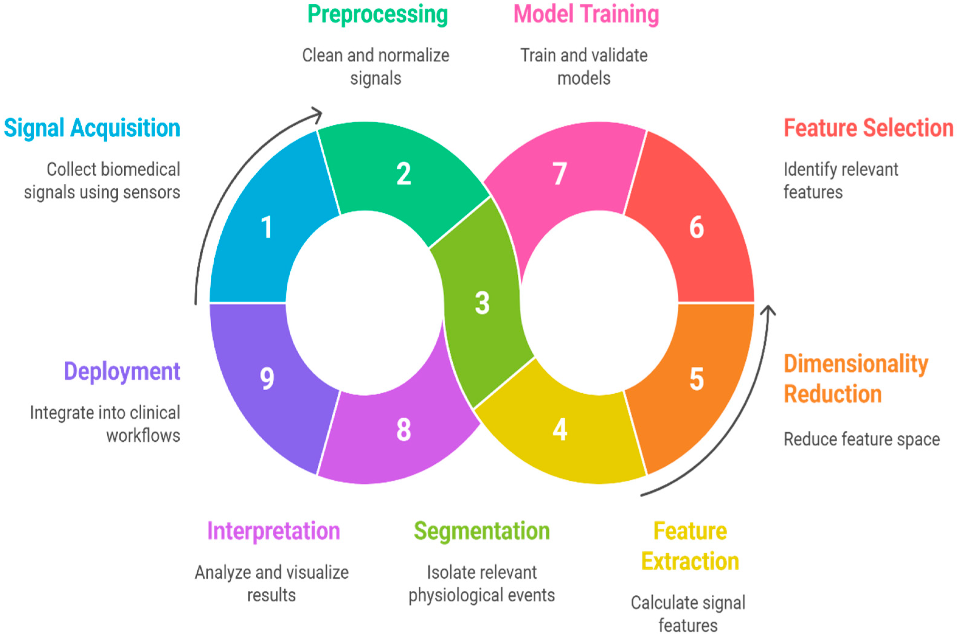
Figure 32. End-to-end workflow for biomedical signal ML, from acquisition and preprocessing to feature engineering, selection, modeling, interpretation, and deployment. Each stage is annotated with standard methods and best benefits and best Practices.
Applsci 15 12036 g032
A well-structured end-to-end workflow:
  • Minimizes information loss between stages,
  • Ensures best practices in both signal processing and machine learning,
  • Supports reproducible science by providing traceable data transformations,
  • Facilitates transparent decision-making, critical for clinical validation and regulatory compliance,
  • Eases transition to multi-modal or hybrid (ML-DL) approaches by defining modular interfaces at each stage.

21. Empirical Results/Benchmarks

Rigorous empirical evaluation is central to establishing the validity and generalizability of traditional ML methods in biomedical signal analysis. This section presents a synthesis of benchmark results from the literature, highlights standardized protocols, and provides comparative insights on algorithmic performance for biomedical datasets.

21.1. Benchmarking Protocols

Benchmarking in biomedical signal processing typically involves partitioning datasets into training, validation, and testing subsets using k-fold cross-validation or hold-out methods to provide unbiased estimates of generalization performance. Public datasets, such as those from PhysioNet [34], BCI Competition [158], and OpenECG [159], are widely used to ensure reproducibility and comparability across studies. Standardized metrics, including accuracy, sensitivity, specificity, F1-score, and AUC-ROC [110]. They are strongly recommended for transparent performance assessment, especially given class imbalance concerns prevalent in medical domains.

21.2. Comparative Algorithmic Performance

Empirical studies consistently demonstrate that the optimal choice of algorithm is highly dependent on the nature of the biomedical signal, the feature set, and the dataset size. Random Forests frequently achieve top classification accuracy for respiratory sound analysis, outperforming single decision trees and KNN due to their robustness to noise and feature redundancy. SVMs excel in high-dimensional datasets such as EEG, where sufficient feature engineering or kernel selection is performed. In arrhythmia detection from ECG, SVM and Random Forest models typically outperform logistic regression and Naive Bayes, especially when features are non-linearly separable. Table 16 summarizes representative performance metrics reported in the literature.
The above results illustrate that, on benchmark datasets, traditional ML methods can deliver robust and clinically meaningful diagnostic accuracy, mainly when supported by thoughtful feature engineering and selection.

21.3. Reproducibility and Open Toolboxes

The adoption of open-source toolboxes such as BioSPPy [160], NeuroKit2 [161], and PyWavelets [162] has streamlined preprocessing and feature engineering, facilitating reproducible benchmarking efforts [11]. However, differences in preprocessing choices, feature definitions, or segmentation schemes still pose challenges to direct performance comparison. Future benchmarking efforts should encourage standardized reporting, sharing of code/scripts, and thorough documentation of data handling protocols.

22. Discussion and Research Directions

The comprehensive review presented in this paper highlights the enduring value and evolving role of traditional machine learning (ML) in biomedical signal analysis, emphasizing its interpretability, clinical transparency, and synergy with domain knowledge. Across multiple modalities, including ECG, EEG, EMG, and tracheal breathing sounds, traditional ML continues to provide a robust framework for transforming raw physiological data into clinically meaningful insights. By integrating structured feature engineering, rigorous feature selection, and model interpretability, this paradigm addresses key limitations that persist in contemporary deep learning approaches, particularly in clinical contexts where explainability and reproducibility are essential [1,2,3,4,5,18,117].
A central theme emerging from this review is that feature engineering serves as the cornerstone of clinical interpretability. Unlike end-to-end deep learning models that abstract the feature-learning process, traditional ML relies on explicit, physiologically grounded descriptors. These handcrafted features, spanning time, frequency, and time–frequency domains, offer a transparent link between the signal’s morphology and underlying physiological mechanisms [18,28,29,30]. This traceability not only enhances clinical trust but also supports regulatory approval, as it enables clinicians to understand and justify model predictions [20,21,78,79]. Moreover, the adaptability of these features across diverse biomedical modalities reinforces the generalizability of traditional ML pipelines, provided that appropriate preprocessing and normalization strategies are applied [13,27,123].
Another critical insight is the interdependence between feature selection and model interpretability. Effective selection strategies, such as filter, wrapper, and embedded methods, not only reduce redundancy but also highlight physiologically relevant variables that contribute most significantly to diagnostic accuracy [50,51,52,53,54,55,56]. Embedded approaches, particularly those integrated into ensemble algorithms like Random Forests or regularized models such as Lasso regression, provide a direct mapping between statistical relevance and clinical meaning [56,61,117]. The capacity to quantify and visualize feature importance bridges the gap between computational analytics and medical reasoning, transforming ML outputs into interpretable evidence for decision support [100,101,105].
The discussion also underscores the balance between interpretability and predictive performance. While deep learning models often surpass traditional ML in large-scale, unstructured datasets, their opaque decision-making remains a significant obstacle for clinical deployment [4,5,9,10]. Traditional ML, although sometimes less performant on raw data, compensates for this by offering transparency and data efficiency, two characteristics that are indispensable in healthcare environments constrained by limited, noisy, or imbalanced datasets [11,12,13,122]. Furthermore, recent advances in explainable AI (XAI) tools such as SHAP and LIME have extended interpretability even to complex ensemble models, reinforcing the practical viability of traditional ML in clinical workflows [105,106,107,112,113].
From a translational perspective, this review affirms that the path toward clinically explainable AI lies in hybridization rather than replacement. The integration of deep learning’s feature extraction capabilities with the interpretability of traditional ML classifiers forms a promising direction for future research [117,144,145]. Such hybrid pipelines can automatically capture high-dimensional representations while maintaining clinician-accessible interpretability through secondary ML layers. This approach aligns regulatory expectations for transparent medical AI systems and holds significant potential for real-time applications in patient monitoring and diagnostics [113,137,142,143].
Nevertheless, several challenges remain unresolved. Traditional ML approaches are limited by their reliance on handcrafted features, scalability constraints, and the difficulty of capturing complex temporal dependencies in long-duration biomedical signals [134,135,136,137]. Addressing these limitations requires methodological innovations that combine automated feature generation, adaptive preprocessing, and robust cross-domain validation [36,139,140,141]. Collaborative frameworks that bring together data scientists, engineers, and clinicians will be essential to ensure that future models are not only statistically sound but also physiologically meaningful and ethically deployable [116,117,139,140,141].
Moreover, this review reinforces that traditional ML remains an indispensable component of biomedical signal analysis. It provides the interpretive foundation necessary for trustworthy, transparent, and clinically relevant artificial intelligence in healthcare. Rather than viewing traditional ML and deep learning as competing paradigms, they should be considered complementary, each addressing different facets of the broader challenge of transforming biosignals into actionable medical knowledge. The next generation of biomedical AI is likely to emerge from this convergence, where interpretable features, validated models, and clinical insights coexist within an integrated, explainable, and patient-centered framework [117,137,142,143,144,145].
Building on this vision, several research directions will shape the continued evolution and clinical translation of traditional ML in biomedical signal analysis. Future work should focus on automating and hybridizing feature engineering through bio-inspired optimization and deep–shallow integration strategies, enabling models to capture salient signal characteristics while retaining interpretability efficiently [116,117,139,140,141]. The development of scalable multimodal and longitudinal frameworks capable of integrating heterogeneous signals such as ECG, EEG, respiratory sounds, and EHR data will be essential for comprehensive patient modeling and disease trajectory analysis [113,137,142,143]. Parallel efforts must strengthen transparency and regulatory compliance by expanding explainability toolkits (e.g., SHAP, LIME) and aligning with emerging standards such as the FDA’s Good Machine Learning Practice, GDPR-compliant governance, and privacy-preserving paradigms like federated learning [1,2,3,4,5,18,117]. Equally important is the promotion of open science through shared datasets, standardized benchmarks, and reproducible pipelines to facilitate collaboration and objective performance comparison across modalities [36,139,140,141]. Finally, the deployment of energy-efficient ML models suitable for wearable and edge devices remains an urgent need, supporting real-time monitoring and early anomaly detection in telemedicine and resource-limited environments [116,117,139,140,141].
A critical direction for advancing traditional ML is the development of automated and domain-informed feature engineering strategies. While handcrafted features have historically ensured interpretability, their manual derivation limits scalability and adaptation to complex or multimodal signals [113,137,142,143]. Future studies can adopt more sophisticated signal processing methodologies, like wavelet, fractal, and entropy-based descriptors, combined with optimization-based feature selection methods, to automatically extract features that capture physiologically meaningful patterns in biomedical signal data. This approach preserves interpretability while enabling models to adapt dynamically to patient-specific or longitudinal variations, addressing the limitations of static feature sets in evolving clinical contexts [116,117,139,140,141].
Another promising avenue is the integration of hybrid deep–shallow architectures, where deep learning extracts high-dimensional latent representations, which are subsequently refined and interpreted using traditional ML classifiers. This allows the capture of complex temporal or spectral patterns while maintaining clinician-accessible reasoning. Similarly, multimodal and longitudinal analysis combining ECG, EEG, respiratory sounds, and EHR data can benefit from hierarchical feature integration, cross-modal regularization, and ensemble-based meta-learning [113,137,142,143]. Such strategies enhance patient-specific modeling, support disease trajectory analysis, and retain physiologically meaningful, interpretable descriptors, providing a clear path for translating ML outputs into actionable clinical insights. Collectively, these directions define a roadmap toward trustworthy, interoperable, and clinically sustainable ML solutions for biomedical signal analysis.

23. Limitations of This Review

This review is limited by its focus on peer-reviewed English-language journal articles, which may exclude relevant conference or non-English studies [2,3,4]. The scope was restricted to traditional machine learning (ML), excluding purely deep learning (DL) approaches, though hybrid ML–DL methods are rapidly emerging [117,144,145]. Differences in datasets, preprocessing, and evaluation metrics across studies also limit direct performance comparisons [122,123,126]. Moreover, most interpretability findings were model-centric, with limited clinical validation [113,117,137]. Future work should address these gaps through standardized benchmarking, multimodal data integration, and collaborative clinician-in-the-loop evaluation.
Additionally, this review provides a synthesis up to mid-2025, and given the rapid pace of advancements in biomedical AI, emerging developments such as federated learning, self-supervised representations, and dynamic explainability frameworks may not yet be reflected [139,140,141,142,143]. Continuous updates to this review will therefore be necessary to capture new methodologies, regulatory guidelines, and interdisciplinary innovations that further strengthen the integration of interpretable ML into clinical practice.

24. Conclusions

Traditional machine learning algorithms continue to hold significant value in analyzing biomedical signals, particularly due to their inherent interpretability and the transparent role of feature engineering. This paper has provided a comprehensive review, emphasizing the critical processes of feature extraction, feature selection, and model interpretation within this domain. We have explored how various time-domain, frequency-domain, and time-frequency domain techniques are employed to derive meaningful features from complex physiological data, including the specialized case of tracheal breathing sounds. The importance of feature selection in reducing dimensionality, mitigating overfitting, and enhancing model performance has been highlighted, along with a discussion of filter, wrapper, and embedded methods. The dedicated section on breathing sound analysis demonstrates how traditional ML techniques can be effectively applied to respiratory health monitoring, providing a non-invasive approach to detecting various respiratory conditions through tracheal breathing sound analysis.
Furthermore, we have detailed the application of widely used traditional ML algorithms such as Support Vector Machines, K-Nearest Neighbors, Decision Trees, and Random Forests in diverse biomedical contexts. A key advantage of these approaches lies in their interpretability, which enables clinicians and researchers to understand the basis of a model’s predictions, a crucial factor for trust and adoption in healthcare settings. The performance comparison section has illustrated the trade-offs between different algorithms and the factors that influence their effectiveness.
Despite the rise in deep learning, traditional ML methods remain relevant, especially in scenarios with limited data, when computational resources are constrained, or when model transparency is paramount. The analysis of tracheal breathing sounds exemplifies how traditional approaches can provide clinically meaningful insights while maintaining interpretability and clarity. While challenges such as the reliance on handcrafted features and sensitivity to noise persist, continuous advancements in signal processing and feature engineering techniques continue to enhance their applicability.
By carefully considering feature engineering, selection, and interpretation, traditional machine learning offers a robust and understandable framework for advancing biomedical signal analysis. The inclusion of breathing sound analysis, particularly tracheal breathing sounds, demonstrates the versatility of these approaches across different types of physiological signals. As healthcare continues to embrace data-driven approaches, traditional ML methods will continue to play a vital role in developing interpretable, trustworthy, and clinically applicable diagnostic tools that contribute significantly to diagnostic accuracy and patient care.

Author Contributions

Conceptualization, A.M.A. and Z.M.; methodology, A.M.A. and Z.M.; software, A.M.A.; validation, A.M.A. and Z.M.; formal analysis, A.M.A. and Z.M.; investigation, A.M.A. and Z.M.; data curation, A.M.A. and Z.M.; writing—original draft preparation, A.M.A.; writing—review and editing, A.M.A. and Z.M.; visualization, A.M.A. and Z.M.; supervision, Z.M.; project administration, Z.M.; funding acquisition, Z.M. All authors have read and agreed to the published version of the manuscript.

Funding

This research was funded by the Natural Sciences and Engineering Research Council of Canada (NSERC).

Institutional Review Board Statement

Not applicable.

Informed Consent Statement

Not applicable.

Data Availability Statement

Not applicable.

Acknowledgments

We acknowledge the support of the NSERC (Natural Sciences and Engineering Research Council of Canada).

Conflicts of Interest

The authors declare no conflicts of interest.

Abbreviations

The following abbreviations are used in this manuscript:
AIArtificial Intelligence
ANNArtificial Neural Network
ANOVAAnalysis of Variance
AUCArea Under the Curve
AUC-ROCArea Under the Receiver Operating Characteristic Curve
AUPRCArea Under the Precision–Recall Curve
BCIBrain–Computer Interface
CFSCorrelation-based Feature Selection
CNNConvolutional Neural Network
COPDChronic Obstructive Pulmonary Disease
CPUCentral Processing Unit
CVCross Validation
CWTContinuous Wavelet Transform
DLDeep Learning
DWTDiscrete Wavelet Transform
ECGElectrocardiogram
ECoGElectrocorticography
EEGElectroencephalogram
EHRElectronic Health Record
EMGElectromyogram
EMRElectronic Medical Record (if mentioned; check consistency with EHR)
EMAEuropean Medicines Agency
EOGElectrooculogram
EVestGElectrovestibulography
FAIRFindable, Accessible, Interoperable and Reusable
FFTFast Fourier Transform
FLFederated Learning
FNFalse Negative
FPFalse Positive
FDAFood and Drug Administration (U.S.)
Grad-CAMGradient-weighted Class Activation Mapping
GPUGraphics Processing Unit
HHTHilbert-Huang Transform
HIPAAHealth Insurance Portability and Accountability Act
HOSHigher-Order Statistics
HRVHeart Rate Variability
ICAIndependent Component Analysis
ICEIndividual Conditional Expectation
ICBHIInternational Conference on Biomedical Health Informatics
KNNK-Nearest Neighbors
LDALinear Discriminant Analysis
LIMELocal Interpretable Model-Agnostic Explanations
LOSOLeave-One-Subject-Out
LOSO-CVLeave-One-Subject-Out Cross Validation
LSTMLong Short-Term Memory
MAEMean Absolute Error
MFCCMel-Frequency Cepstral Coefficients
MIT-BIHMassachusetts Institute of Technology–Beth Israel Hospital (ECG dataset)
MLMachine Learning
MSEMean Squared Error
NinaproNon-Invasive Adaptive Prosthetics (EMG dataset)
Ninapro EMGNinapro EMG dataset
OSAObstructive Sleep Apnea
PCAPrincipal Component Analysis
PDPPartial Dependence Plot
PPGPhotoplethysmogram
PSDPower Spectral Density
QRSQRS Complex (ECG feature)
RBFRadial Basis Function
RFERecursive Feature Elimination
RNNRecurrent Neural Network
RMSERoot Mean Squared Error
RMSRoot Mean Square
SVMSupport Vector Machine
STFTShort-Time Fourier Transform
σStandard Deviation (used symbolically in quantitative analysis)
TBSTracheal Breathing Sound
TPTrue Positive
TNTrue Negative
TUHTemple University Hospital (EEG dataset)
TUH-EEGTemple University Hospital EEG dataset (used in benchmarking)
WTWavelet Transform
XAIExplainable Artificial Intelligence
XGB or XGBoostExtreme Gradient Boosting
ZCRZero-Crossing Rate

References

  1. Alqudah, A.M.; Moussavi, Z. A Review of Deep Learning for Biomedical Signals: Current Applications, Advancements, Future Prospects, Interpretation, and Challenges. Comput. Mater. Contin. 2025, 83, 3753–3841. [Google Scholar] [CrossRef]
  2. Faust, O.; Hagiwara, Y.; Hong, T.J.; Lih, O.S.; Acharya, U.R. Deep learning for healthcare applications based on physiological signals: A review. Comput. Methods Programs Biomed. 2018, 161, 1–13. [Google Scholar] [CrossRef]
  3. Lal, T.N.; Schröder, M.; Hinterberger, T.; Weston, J.; Bogdan, M.; Birbaumer, N.; Schölkopf, B. Support Vector Channel Selection in BCI. IEEE Trans. Biomed. Eng. 2004, 51, 1003–1010. [Google Scholar] [CrossRef]
  4. Domingos, P. A Few Useful Things to Know about Machine Learning. Commun. ACM 2012, 55, 78–87. [Google Scholar] [CrossRef]
  5. Guyon, I.; Elisseeff, A. An Introduction to Variable and Feature Selection. J. Mach. Learn. Res. 2003, 3, 1157–1182. [Google Scholar]
  6. Lipton, Z.C. The Mythos of Model Interpretability. Queue 2018, 16, 31–57. [Google Scholar] [CrossRef]
  7. Dobson, A.J.; Barnett, A.G. An Introduction to Generalized Linear Models, 3rd ed.; Chapman and Hall/CRC: Boca Raton, FL, USA, 2008. [Google Scholar]
  8. Hosmer, D.W., Jr.; Lemeshow, S.; Sturdivant, R.X. Applied Logistic Regression, 3rd ed.; Wiley: Hoboken, NJ, USA, 2013. [Google Scholar]
  9. Adadi, A.; Berrada, M. Peeking inside the Black-Box: A Survey on Explainable Artificial Intelligence (XAI). IEEE Access 2018, 6, 52138–52160. [Google Scholar] [CrossRef]
  10. Molnar, C. Interpretable Machine Learning: A Guide for Making Black Box Models Explainable, 2nd ed.; Chapman & Hall/CRC: Boca Raton, FL, USA, 2022. [Google Scholar]
  11. Mahmood, F. A Benchmarking Crisis in Biomedical Machine Learning. Nat. Med. 2025, 31, 1060. [Google Scholar] [CrossRef]
  12. Piirilä, P.; Sovijärvi, A.R.A. Crackles: Recording, Analysis and Clinical Significance. Eur. Respir. J. 1995, 8, 2139–2148. [Google Scholar] [CrossRef] [PubMed]
  13. Gallón, V.M.; Vélez, S.M.; Ramírez, J.; Bolaños, F. Comparison of Machine Learning Algorithms and Feature Extraction Techniques for the Automatic Detection of Surface EMG Activation Timing. Biomed. Signal Process. Control. 2024, 94, 106266. [Google Scholar] [CrossRef]
  14. Wang, S.; Jiang, Y.; Li, Q.; Zhang, W. Timely ICU Outcome Prediction Utilizing Stochastic Signal Analysis and Machine Learning Techniques with Readily Available Vital Sign Data. IEEE J. Biomed. Health Inform. 2024, 28, 4123–4134. [Google Scholar] [CrossRef] [PubMed]
  15. Bohadana, A.; Izbicki, G.; Kraman, S.S. Fundamentals of Lung Auscultation. N. Engl. J. Med. 2014, 370, 744–751. [Google Scholar] [CrossRef] [PubMed]
  16. Richman, J.S.; Moorman, J.R. Physiological Time-Series Analysis Using Approximate Entropy and Sample Entropy. Am. J. Physiol.-Heart Circ. Physiol. 2000, 278, H2039–H2049. [Google Scholar] [CrossRef] [PubMed]
  17. Huang, N.E.; Shen, Z.; Long, S.R.; Wu, M.C.; Shih, H.H.; Zheng, Q.; Yen, N.C.; Tung, C.C.; Liu, H.H. The Empirical Mode Decomposition and the Hilbert Spectrum for Nonlinear and Non-Stationary Time Series Analysis. Proc. R. Soc. London Ser. A Math. Phys. Eng. Sci. 1998, 454, 903–995. [Google Scholar] [CrossRef]
  18. Subasi, A.; Qaisar, S.M. Signal Acquisition Preprocessing and Feature Extraction Techniques for Biomedical Signals. In Advances in Non-Invasive Biomedical Signal Processing; Springer: Berlin/Heidelberg, Germany, 2023; pp. 11–34. [Google Scholar]
  19. Rangayyan, R.M. Biomedical Signal Analysis: A Case-Study Approach, 2nd ed.; Wiley-IEEE Press: Hoboken, NJ, USA, 2015. [Google Scholar]
  20. U.S. Food and Drug Administration. Artificial Intelligence/Machine Learning (AI/ML)-Based Software as a Medical Device (SaMD) Action Plan. 2021. Available online: https://www.fda.gov/medical-devices/software-medical-device-samd/artificial-intelligence-software-medical-device (accessed on 1 May 2025).
  21. European Medicines Agency. Reflection Paper on Artificial Intelligence (AI) in Medicines. 2022. Available online: https://www.ema.europa.eu/en/news/reflection-paper-use-artificial-intelligence-lifecycle-medicines#:~:text=The%20reflection%20paper%20highlights%20that,due%20respect%20of%20fundamental%20rights (accessed on 1 May 2025).
  22. Cascarano, A.; Mur-Petit, J.; Hernández-González, J.; Camacho, M.; De Toro Eadie, N.; Gkontra, P.; Chadeau-Hyam, M.; Vitrià, J.; Lekadir, K. Machine and Deep Learning for Longitudinal Biomedical Data: A Review of Methods and Applications. Artif. Intell. Rev. 2023, 56, 1711–1771. [Google Scholar] [CrossRef]
  23. Lee, Y.J.; Park, C.; Kim, H.; Cho, S.J.; Yeo, W.-H. Artificial Intelligence on Biomedical Signals: Technologies, Applications, and Future Directions. Med-X 2024, 2, 25. [Google Scholar] [CrossRef]
  24. Toledo-Pérez, D.C.; Rodríguez-Reséndiz, J.; Gómez-Loenzo, R.A.; Jauregui-Correa, J.C. Support Vector Machine-Based EMG Signal Classification Techniques: A Review. Appl. Sci. 2019, 9, 4402. [Google Scholar] [CrossRef]
  25. Nguyen, M.T.; Nguyen, T.-H.T.; Le, H.-C. A Review of Progress and an Advanced Method for Shock Advice Algorithms in Automated External Defibrillators. Biomed. Eng. OnLine 2022, 21, 22. [Google Scholar] [CrossRef]
  26. Zhang, X.; Wang, L.; Chen, Y. A Review of Deep Learning-Based Approaches for EMG Signal Analysis. J. Neural Eng. 2019, 16, 051001. [Google Scholar]
  27. Azarbarzin, A.; Moussavi, Z.M.K. Automatic and Unsupervised Snore Sound Extraction from Respiratory Sound Signals. IEEE Trans. Biomed. Eng. 2010, 57, 2446–2453. [Google Scholar] [CrossRef]
  28. Singh, A.K.; Krishnan, S. ECG Signal Feature Extraction Trends in Methods and Applications. Biomed. Eng. OnLine 2023, 22, 22. [Google Scholar] [CrossRef] [PubMed]
  29. Kim, H.; Kon, D.; Jung, Y.; Han, H.; Kim, J.; Joo, Y. Breathing Sounds Analysis System for Early Detection of Airway Problems in Patients with a Tracheostomy Tube. Sci. Rep. 2023, 13, 21013. [Google Scholar] [CrossRef]
  30. Subasi, A. Practical Guide for Biomedical Signals Analysis Using Machine Learning Techniques: A MATLAB Based Approach; Academic Press: Cambridge, MA, USA, 2019. [Google Scholar]
  31. Folland, R.; Hines, E.; Dutta, R.; Boilot, P. Comparison of Neural Network Predictors in the Classification of Tracheal–Bronchial Breath Sounds by Respiratory Auscultation. Artif. Intell. Med. 2004, 31, 211–220. [Google Scholar] [CrossRef] [PubMed]
  32. Li, X.; Ling, S.H.; Su, S. A Hybrid Feature Selection and Extraction Method for Sleep Apnea Detection Using Bio-Signals. Sensors 2020, 20, 4323. [Google Scholar] [CrossRef]
  33. Karim, A.; Ryu, S.; Jeong, I.C. Ensemble Learning for Biomedical Signal Classification: A High-Accuracy Framework Using Spectrograms from Percussion and Palpation. Sci. Rep. 2025, 15, 21592. [Google Scholar] [CrossRef]
  34. Goldberger, A.L.; Amaral, L.A.; Glass, L.; Hausdorff, J.M.; Ivanov, P.C.; Mark, R.G.; Mietus, J.E.; Moody, G.B.; Peng, C.K.; Stanley, H.E. PhysioBank, PhysioToolkit, and PhysioNet: Components of a New Research Resource for Complex Physiologic Signals. Circulation 2000, 101, e215–e220. [Google Scholar] [CrossRef] [PubMed]
  35. Boronoev, V.V.; Ompokov, V.D. The Hilbert-Huang Transform for Biomedical Signals Processing. In Proceedings of the 2014 International Conference on Computer Technologies in Physical and Engineering Applications (ICCTPEA), Saint-Petersburg, Russia, 24–26 June 2014; pp. 21–22. [Google Scholar]
  36. Costa, M.; Goldberger, A.L.; Peng, C.K. Multiscale Entropy Analysis of Complex Physiologic Time Series. Phys. Rev. Lett. 2002, 89, 068102. [Google Scholar] [CrossRef]
  37. Amin, H.U.; Malik, A.S.; Ahmad, R.F.; Badruddin, N.; Kamel, N.; Hussain, M.; Chooi, W.T. Feature Extraction and Classification for EEG Signals Using Wavelet Transform and Machine Learning Techniques. Australas. Phys. Eng. Sci. Med. 2015, 38, 139–149. [Google Scholar] [CrossRef]
  38. Charlton, P.H.; Harana, J.M.; Vennin, S.; Li, Y.; Chowienczyk, P.; Alastruey, J. Modeling Arterial Pulse Waves in Healthy Aging: A Database for in Silico Evaluation of Hemodynamics and Pulse Wave Indexes. Am. J. Physiol.-Heart Circ. Physiol. 2019, 317, H1062–H1085. [Google Scholar] [CrossRef]
  39. Rosenstein, M.T.; Collins, J.J.; De Luca, C.J. A Practical Method for Calculating Largest Lyapunov Exponents from Small Data Sets. Phys. D Nonlinear Phenom. 1993, 65, 117–134. [Google Scholar] [CrossRef]
  40. Abdelhamid, A.A.; El-Kenawy, E.-S.M.; Alotaibi, B.; Amer, G.M.; Abdelkader, M.Y.; Ibrahim, A.; Eid, M.M. Robust Speech Emotion Recognition Using CNN+LSTM Based on Stochastic Fractal Search Optimization Algorithm. IEEE Access 2022, 10, 49265–49284. [Google Scholar] [CrossRef]
  41. Hajipour, F.; Moussavi, Z. Spectral and Higher Order Statistical Characteristics of Expiratory Tracheal Breathing Sounds During Wakefulness and Sleep in People with Different Levels of Obstructive Sleep Apnea. J. Med. Biol. Eng. 2019, 39, 244–250. [Google Scholar] [CrossRef]
  42. Mendel, J.M. Tutorial on Higher-Order Statistics (Spectra) in Signal Processing and System Theory: Theoretical Results and Some Applications. Proc. IEEE 1991, 79, 278–305. [Google Scholar] [CrossRef]
  43. Nikias, C.L.; Petropulu, A.P. Higher-Order Spectra Analysis: A Nonlinear Signal Processing Framework; Prentice Hall: Hoboken, NJ, USA, 1993. [Google Scholar]
  44. Ashwini, A.; Chirchi, V.; Balasubramaniam, S.; Shah, M.A. Bio Inspired Optimization Techniques for Disease Detection in Deep Learning Systems. Sci. Rep. 2025, 15, 18202. [Google Scholar] [CrossRef]
  45. Sahu, P.; Singh, B.K.; Nirala, N. An Improved Feature Selection Approach Using Global Best Guided Gaussian Artificial Bee Colony for EMG Classification. Biomed. Signal Process. Control. 2023, 80, 104399. [Google Scholar] [CrossRef]
  46. Li, H.; Yuan, D.; Ma, X.; Cui, D.; Cao, L. Genetic Algorithm for the Optimization of Features and Neural Networks in ECG Signals Classification. Sci. Rep. 2017, 7, 41011. [Google Scholar] [CrossRef]
  47. Sultana, A.; Ahmed, F.; Alam, M.S. A Systematic Review on Surface Electromyography-Based Classification System for Identifying Hand and Finger Movements. Healthc. Anal. 2023, 3, 100126. [Google Scholar] [CrossRef]
  48. Li, Q.; Liu, C.; Oster, J.; Clifford, G.D. Signal Processing and Feature Selection Preprocessing for Classification in Noisy Healthcare Data. In Machine Learning for Healthcare; NIH: Bethesda, MD, USA, 2016. [Google Scholar]
  49. Remeseiro, B.; Bolón-Canedo, V. A Review of Feature Selection Methods in Medical Applications. Comput. Biol. Med. 2019, 112, 103375. [Google Scholar] [CrossRef]
  50. Hall, M.A. Correlation-Based Feature Selection for Discrete and Numeric Class Machine Learning. In Proceedings of the Seventeenth International Conference on Machine Learning, San Francisco, CA, USA, 29 June–2 July 2000; pp. 359–366. [Google Scholar]
  51. Friedman, J.H. Greedy Function Approximation: A Gradient Boosting Machine. Ann. Stat. 2001, 29, 1189–1232. [Google Scholar] [CrossRef]
  52. Hastie, T.; Tibshirani, R.; Friedman, J. The Elements of Statistical Learning: Data Mining, Inference, and Prediction, 2nd ed.; Springer: Berlin/Heidelberg, Germany, 2009. [Google Scholar]
  53. Guyon, I.; Weston, J.; Barnhill, S.; Vapnik, V. Gene Selection for Cancer Classification Using Support Vector Machines. Mach. Learn. 2002, 46, 389–422. [Google Scholar] [CrossRef]
  54. Tibshirani, R. Regression Shrinkage and Selection via the Lasso. J. R. Stat. Soc. Ser. B (Methodol.) 1996, 58, 267–288. [Google Scholar] [CrossRef]
  55. Breiman, L. Random Forests. Mach. Learn. 2001, 45, 5–32. [Google Scholar] [CrossRef]
  56. Cortes, C.; Vapnik, V. Support-Vector Networks. Mach. Learn. 1995, 20, 273–297. [Google Scholar] [CrossRef]
  57. Haykin, S. Neural Networks and Learning Machines, 3rd ed.; Pearson: Hoboken, NJ, USA, 2008. [Google Scholar]
  58. Qaisar, S.M.; Nisar, H.; Subasi, A. Advances in Non-Invasive Biomedical Signal Sensing and Processing with Machine Learning; Springer: Berlin/Heidelberg, Germany, 2023. [Google Scholar]
  59. Sperandei, S. Understanding Logistic Regression Analysis. Biochem. Med. 2014, 24, 12–18. [Google Scholar] [CrossRef] [PubMed]
  60. Wasimuddin, M.; Elleithy, K.; Abuzneid, A.S. Stages-Based ECG Signal Analysis from Traditional Signal Processing to Machine Learning Approaches: A Survey. IEEE Access 2020, 8, 177782–177803. [Google Scholar] [CrossRef]
  61. Lundberg, S.M.; Lee, S.-I. A Unified Approach to Interpreting Model Predictions. In Proceedings of the Advances in Neural Information Processing Systems, Long Beach, CA, USA, 4–9 December 2017; Volume 30. [Google Scholar]
  62. Suleiman, A.; Lithgow, B.; Mansouri, B.; Moussavi, Z. Investigating the Validity and Reliability of Electrovestibulography (EVestG) for Detecting Post-Concussion Syndrome (PCS) with and without Comorbid Depression. Sci. Rep. 2018, 8, 14495. [Google Scholar] [CrossRef]
  63. Dastgheib, Z.A.; Kumaragamage, C.; Lithgow, B.J.; Moussavi, Z.K. The Evolution of Electrovestibulography Technique and Safety Considerations. Biomed. Eng. Adv. 2025, 9, 100157. [Google Scholar] [CrossRef]
  64. Ribeiro, M.T.; Singh, S.; Guestrin, C. Why Should I Trust You?: Explaining the Predictions of Any Classifier. In Proceedings of the 22nd ACM SIGKDD International Conference on Knowledge Discovery and Data Mining, San Francisco, CA, USA, 13–17 August 2016; pp. 1135–1144. [Google Scholar]
  65. Sahoo, R.R.; Bhowmick, S.; Mandal, D.; Kumar Kundu, P. A Novel Approach of Gaussian Mixture Model-Based Data Compression of ECG and PPG Signals for Various Cardiovascular Diseases. Biomed. Signal Process. Control. 2024, 96, 106581. [Google Scholar] [CrossRef]
  66. Dhyani, S.; Kumar, A.; Choudhury, S. Analysis of ECG-Based Arrhythmia Detection System Using Machine Learning. MethodsX 2023, 10, 102195. [Google Scholar] [CrossRef] [PubMed]
  67. Richhariya, B.; Tanveer, M. EEG Signal Classification Using Universum Support Vector Machine. Expert Syst. Appl. 2018, 106, 169–182. [Google Scholar] [CrossRef]
  68. Cinyol, F.; Baysal, U.; Köksal, D.; Babaoğlu, E.; Ulaşlı, S.S. Incorporating Support Vector Machine to the Classification of Respiratory Sounds by Convolutional Neural Network. Biomed. Signal Process. Control. 2023, 79, 104093. [Google Scholar] [CrossRef]
  69. Ashiri, M.; Lithgow, B.; Suleiman, A.; Mansouri, B.; Moussavi, Z. Electrovestibulography (EVestG) Application for Measuring Vestibular Response to Horizontal Pursuit and Saccadic Eye Movements. Biocybern. Biomed. Eng. 2021, 41, 527–539. [Google Scholar] [CrossRef]
  70. Dastgheib, Z.A.; Lithgow, B.J.; Moussavi, Z.K. Evaluating the Diagnostic Value of Electrovestibulography (EVestG) in Alzheimer’s Patients with Mixed Pathology: A Pilot Study. Medicina 2023, 59, 2091. [Google Scholar] [CrossRef]
  71. Sha’abani, M.N.A.H.; Fuad, N.; Jamal, N.; Ismail, M.F. kNN and SVM Classification for EEG: A Review. In InECCE2019; Lecture Notes in Electrical Engineering; Kasruddin Nasir, A.N., Ahmad, M.A., Najib, M.S., Abdul Wahab, Y., Othman, N.A., Abd Ghani, N.M., Irawan, A., Khatun, S., Raja Ismail, R.M.T., Saari, M.M., et al., Eds.; Springer: Singapore, 2020; Volume 632, pp. 555–565. ISBN 978-981-15-2316-8. [Google Scholar]
  72. Hassaballah, M.; Wazery, Y.M.; Ibrahim, I.E.; Farag, A. ECG Heartbeat Classification Using Machine Learning and Metaheuristic Optimization for Smart Healthcare Systems. Bioengineering 2023, 10, 429. [Google Scholar] [CrossRef] [PubMed]
  73. Satapathy, S.K.; Thakkar, S.; Patel, A.; Patel, D.; Patel, D. An Effective EEG Signal-Based Sleep Staging System Using Machine Learning Techniques. In Proceedings of the 2022 IEEE 6th Conference on Information and Communication Technology (CICT), Gwalior, India, 18 November 2022; pp. 1–6. [Google Scholar]
  74. Chen, C.-H.; Huang, W.-T.; Tan, T.-H.; Chang, C.-C.; Chang, Y.-J. Using K-Nearest Neighbor Classification to Diagnose Abnormal Lung Sounds. Sensors 2015, 15, 13132–13158. [Google Scholar] [CrossRef]
  75. Langley, P.; Iba, W.; Thompson, K. An Analysis of Bayesian Classifiers. In Proceedings of the Tenth National Conference on Artificial Intelligence, San Jose, CA, USA, 12–16 July 1992; pp. 223–228. [Google Scholar]
  76. Sabry, A.H.; Dallal Bashi, O.I.; Nik Ali, N.H.; Mahmood Al Kubaisi, Y. Lung Disease Recognition Methods Using Audio-Based Analysis with Machine Learning. Heliyon 2024, 10, e26218. [Google Scholar] [CrossRef]
  77. Satapathy, S.K.; Brahma, B.; Panda, B.; Barsocchi, P.; Bhoi, A.K. Machine Learning-Empowered Sleep Staging Classification Using Multi-Modality Signals. BMC Med. Inform. Decis. Mak. 2024, 24, 119. [Google Scholar] [CrossRef] [PubMed]
  78. Ahsan, M.M.; Luna, S.A.; Siddique, Z. Machine-Learning-Based Disease Diagnosis: A Comprehensive Review. Healthcare 2022, 10, 541. [Google Scholar] [CrossRef]
  79. Dash, T.K.; Chakraborty, C.; Mahapatra, S.; Panda, G. Gradient Boosting Machine and Efficient Combination of Features for Speech-Based Detection of COVID-19. IEEE J. Biomed. Health Inform. 2022, 26, 5364–5371. [Google Scholar] [CrossRef]
  80. Türkmen, G.; Sezen, A. A Comparative Analysis of XGBoost and LightGBM Approaches for Human Activity Recognition: Speed and Accuracy Evaluation. IJCESEN 2024, 10, 329. [Google Scholar] [CrossRef]
  81. Zheng, Y.; Guo, X.; Yang, Y.; Wang, H.; Liao, K.; Qin, J. Phonocardiogram Transfer Learning-Based CatBoost Model for Diastolic Dysfunction Identification Using Multiple Domain-Specific Deep Feature Fusion. Comput. Biol. Med. 2023, 156, 106707. [Google Scholar] [CrossRef]
  82. Abdullah; Fatima, Z.; Abdullah, J.; Rodríguez, J.L.O.; Sidorov, G. A Multimodal AI Framework for Automated Multiclass Lung Disease Diagnosis from Respiratory Sounds with Simulated Biomarker Fusion and Personalized Medication Recommendation. IJMS 2025, 26, 7135. [Google Scholar] [CrossRef]
  83. Shamout, F.; Zhu, T.; Clifton, D.A. Machine Learning for Clinical Outcome Prediction. IEEE Rev. Biomed. Eng. 2020, 14, 116–126. [Google Scholar] [CrossRef]
  84. Sezgin, M.C.; Dokur, Z.; Olmez, T.; Korurek, M. Classification of Respiratory Sounds by Using an Artificial Neural Network. In Proceedings of the 2001 Conference Proceedings of the 23rd Annual International Conference of the IEEE Engineering in Medicine and Biology Society, Istanbul, Turkey, 25–28 October 2001; Volume 1, pp. 697–699. [Google Scholar]
  85. Venkatesh, K.; Geetha, S. Sleep Stages Classification Using Artificial Neural Network. Indian J. Sci. Technol. 2015, 8, 31. [Google Scholar] [CrossRef]
  86. Anwaitu Fraser, E.; Obikwelu, O.R. Artificial Neural Networks for Medical Diagnosis: A Review of Recent Trends. Int. J. Comput. Sci. Eng. 2020, 11, 1–11. [Google Scholar] [CrossRef]
  87. Liu, M.; Liu, J.; Xu, M.; Liu, Y.; Li, J.; Nie, W.; Yuan, Q. Combining Meta and Ensemble Learning to Classify EEG for Seizure Detection. Sci. Rep. 2025, 15, 10755. [Google Scholar] [CrossRef] [PubMed]
  88. Sultan, S.Q.; Javaid, N.; Alrajeh, N.; Aslam, M. Machine Learning-Based Stacking Ensemble Model for Prediction of Heart Disease with Explainable AI and K-Fold Cross-Validation: A Symmetric Approach. Symmetry 2025, 17, 185. [Google Scholar] [CrossRef]
  89. Dimigen, O. Optimizing the ICA-Based Removal of Ocular EEG Artifacts from Free Viewing Experiments. NeuroImage 2020, 207, 116117. [Google Scholar] [CrossRef]
  90. Udayana, I.P.A.E.D.; Sudarma, M.; Putra, I.K.G.D.; Sukarsa, I.M.; Jo, M. Comparative Analysis of Denoising Techniques for Optimizing EEG Signal Processing. LKJITI 2025, 15, 124. [Google Scholar] [CrossRef]
  91. Abreu, M.; Fred, A.; Valente, J.; Wang, C.; Plácido Da Silva, H. Morphological Autoencoders for Apnea Detection in Respiratory Gating Radiotherapy. Comput. Methods Programs Biomed. 2020, 195, 105675. [Google Scholar] [CrossRef] [PubMed]
  92. Hu, W.; Lv, J.; Liu, D.; Chen, Y. Unsupervised Feature Learning for Heart Sounds Classification Using Autoencoder. J. Phys. Conf. Ser. 2018, 1004, 012002. [Google Scholar] [CrossRef]
  93. Al-Qazzaz, N.K.; Hamid Bin Mohd Ali, S.; Ahmad, S.A.; Islam, M.S.; Escudero, J. Automatic Artifact Removal in EEG of Normal and Demented Individuals Using ICA-WT during Working Memory Tasks. Sensors 2017, 17, 1326. [Google Scholar] [CrossRef]
  94. Gu, Q.; Li, Z.; Han, J. Linear Discriminant Dimensionality Reduction. In Machine Learning and Knowledge Discovery in Databases; Lecture Notes in Computer Science; Gunopulos, D., Hofmann, T., Malerba, D., Vazirgiannis, M., Eds.; Springer: Berlin/Heidelberg, Germany, 2011; Volume 6911, pp. 549–564. ISBN 978-3-642-23779-9. [Google Scholar]
  95. Subasi, A.; Ismail Gursoy, M. EEG Signal Classification Using PCA, ICA, LDA and Support Vector Machines. Expert Syst. Appl. 2010, 37, 8659–8666. [Google Scholar] [CrossRef]
  96. Tripathy, B.K.; Anveshrithaa, S.; Ghela, S. T-Distributed Stochastic Neighbor Embedding (t-SNE). In Unsupervised Learning Approaches for Dimensionality Reduction and Data Visualization; CRC Press: Boca Raton, FL, USA, 2021. [Google Scholar]
  97. Yang, Y.; Sun, H.; Zhang, Y.; Zhang, T.; Gong, J.; Wei, Y.; Duan, Y.-G.; Shu, M.; Yang, Y.; Wu, D.; et al. Dimensionality Reduction by UMAP Reinforces Sample Heterogeneity Analysis in Bulk Transcriptomic Data. Cell Rep. 2021, 36, 109442. [Google Scholar] [CrossRef] [PubMed]
  98. Sadiq, M.T.; Yu, X.; Yuan, Z. Exploiting Dimensionality Reduction and Neural Network Techniques for the Development of Expert Brain–Computer Interfaces. Expert Syst. Appl. 2021, 164, 114031. [Google Scholar] [CrossRef]
  99. Dadu, A.; Satone, V.K.; Kaur, R.; Koretsky, M.J.; Iwaki, H.; Qi, Y.A.; Ramos, D.M.; Avants, B.; Hesterman, J.; Gunn, R.; et al. Application of Aligned-UMAP to Longitudinal Biomedical Studies. Patterns 2023, 4, 100741. [Google Scholar] [CrossRef]
  100. Shapley, L.S. A Value for N-Person Games. Contrib. Theory Games 1953, 2, 307–317. [Google Scholar]
  101. Wei, P.; Lu, Z.; Song, J. Variable Importance Analysis: A Comprehensive Review. Reliab. Eng. Syst. Saf. 2015, 142, 399–432. [Google Scholar] [CrossRef]
  102. Herbinger, J.; Bischl, B.; Casalicchio, G. REPID: Regional Effect Plots with Implicit Interaction Detection. arXiv 2022, arXiv:2202.07254. [Google Scholar] [CrossRef]
  103. Herbinger, J.; Wright, M.N.; Nagler, T.; Bischl, B.; Casalicchio, G. Decomposing Global Feature Effects Based on Feature Interactions. J. Mach. Learn. Res. 2024, 25, 1–65. [Google Scholar]
  104. Goldstein, A.; Kapelner, A.; Bleich, J.; Pitkin, E. Peeking Inside the Black Box: Visualizing Statistical Learning with Plots of Individual Conditional Expectation. J. Comput. Graph. Stat. 2015, 24, 44–65. [Google Scholar] [CrossRef]
  105. Gramegna, A.; Giudici, P. Shapley Feature Selection. FinTech 2022, 1, 72–80. [Google Scholar] [CrossRef]
  106. Wang, H.; Liang, Q.; Hancock, J.T.; Khoshgoftaar, T.M. Feature Selection Strategies: A Comparative Analysis of SHAP-Value and Importance-Based Methods. J. Big Data 2024, 11, 44. [Google Scholar] [CrossRef]
  107. Lundberg, S.M.; Erion, G.; Chen, H.; DeGrave, A.; Prutkin, J.M.; Nair, B.; Katz, R.; Himmelfarb, J.; Bansal, N.; Lee, S.I. From Local Explanations to Global Understanding with Explainable AI for Trees. Nat. Mach. Intell. 2020, 2, 56–67. [Google Scholar] [CrossRef] [PubMed]
  108. Midway, S.R. Principles of Effective Data Visualization. Patterns 2020, 1, 100141. [Google Scholar] [CrossRef]
  109. Nguyen, Q.V.; Miller, N.; Arness, D.; Huang, W.; Huang, M.L.; Simoff, S. Evaluation on Interactive Visualization Data with Scatterplots. Vis. Inform. 2020, 4, 1–10. [Google Scholar] [CrossRef]
  110. Sathyanarayanan, S. Confusion Matrix-Based Performance Evaluation Metrics. AJBR 2024, 27, 4023–4031. [Google Scholar] [CrossRef]
  111. Davis, J.; Goadrich, M. The Relationship between Precision-Recall and ROC Curves. In Proceedings of the 23rd International Conference on Machine Learning-ICML ’06, Pittsburgh, PA, USA, 25–29 June 2006; pp. 233–240. [Google Scholar]
  112. Lee, Y.; Seo, J. Suggestion of Statistical Validation on Feature Importance of Machine Learning. In Proceedings of the 2023 45th Annual International Conference of the IEEE Engineering in Medicine & Biology Society (EMBC), Sydney, Australia, 24 July 2023; pp. 1–4. [Google Scholar]
  113. Schwartz, J.M.; Moy, A.J.; Rossetti, S.C.; Elhadad, N.; Cato, K.D. Clinician Involvement in Research on Machine Learning–Based Predictive Clinical Decision Support for the Hospital Setting: A Scoping Review. J. Am. Med. Inform. Assoc. 2021, 28, 653–663. [Google Scholar] [CrossRef]
  114. Seoni, S.; Jahmunah, V.; Salvi, M.; Barua, P.D.; Molinari, F.; Acharya, U.R. Application of Uncertainty Quantification to Artificial Intelligence in Healthcare: A Review of Last Decade (2013–2023). Comput. Biol. Med. 2023, 165, 107441. [Google Scholar] [CrossRef]
  115. Feng, J.; Liang, J.; Qiang, Z.; Hao, Y.; Li, X.; Li, L.; Chen, Q.; Liu, G.; Wei, H. A Hybrid Stacked Ensemble and Kernel SHAP-Based Model for Intelligent Cardiotocography Classification and Interpretability. BMC Med. Inform. Decis. Mak. 2023, 23, 273. [Google Scholar] [CrossRef]
  116. Liu, J.; Zhu, D.; Deng, L.; Chen, X. Predictive Modeling of Heart Failure Outcomes Using ECG Monitoring Indicators and Machine Learning. Noninvasive Electrocardiol 2025, 30, e70097. [Google Scholar] [CrossRef] [PubMed]
  117. Sathyan, A.; Weinberg, A.I.; Cohen, K. Interpretable AI for Bio-Medical Applications. Complex Eng. Syst. 2022, 2, 18. [Google Scholar] [CrossRef] [PubMed]
  118. Baldazzi, G.; Solinas, G.; Del Valle, J.; Barbaro, M.; Micera, S.; Raffo, L.; Pani, D. Systematic Analysis of Wavelet Denoising Methods for Neural Signal Processing. J. Neural Eng. 2020, 17, 066016. [Google Scholar] [CrossRef]
  119. Chen, C.-C.; Tsui, F.R. Comparing Different Wavelet Transforms on Removing Electrocardiogram Baseline Wanders and Special Trends. BMC Med. Inform. Decis. Mak. 2020, 20, 343. [Google Scholar] [CrossRef]
  120. Guhdar, M.; Mstafa, R.J.; Mohammed, A.O. A Novel Data Augmentation Strategy for Robust Deep Learning Classification of Biomedical Time-Series Data: Application to ECG and EEG Analysis. arXiv 2025, arXiv:2507.12645. [Google Scholar] [CrossRef]
  121. Bishop, C.M. Pattern Recognition and Machine Learning; Springer: Berlin/Heidelberg, Germany, 2006. [Google Scholar]
  122. Azizi, T. Comparative Analysis of Statistical, Time–Frequency, and SVM Techniques for Change Detection in Nonlinear Biomedical Signals. Signals 2024, 5, 741–761. [Google Scholar] [CrossRef]
  123. Elwali, A.; Moussavi, Z. Obstructive Sleep Apnea Screening and Airway Structure Characterization During Wakefulness Using Tracheal Breathing Sounds. Ann. Biomed. Eng. 2017, 45, 839–850. [Google Scholar] [CrossRef]
  124. Quinlan, J.R. Induction of Decision Trees. Mach. Learn. 1986, 1, 81–106. [Google Scholar] [CrossRef]
  125. Gammerman, A.; Shafer, G.; Vovk, V. Algorithmic Learning in a Random World; Springer-Verlag: Berlin/Heidelberg, Germany, 2005; ISBN 0-387-00152-2. [Google Scholar]
  126. Elwali, A.; Moussavi, Z. A Novel Decision Making Procedure during Wakefulness for Screening Obstructive Sleep Apnea Using Anthropometric Information and Tracheal Breathing Sounds. Sci. Rep. 2019, 9, 11467. [Google Scholar] [CrossRef]
  127. Islam, T.; Basak, M.; Islam, R.; Roy, A.D. Investigating Population-Specific Epilepsy Detection from Noisy EEG Signals Using Deep-Learning Models. Heliyon 2023, 9, e22208. [Google Scholar] [CrossRef]
  128. Saha Tchinda, B.; Tchiotsop, D. A Lightweight 1D Convolutional Neural Network Model for Arrhythmia Diagnosis from Electrocardiogram Signal. Phys. Eng. Sci. Med. 2025, 48, 577–589. [Google Scholar] [CrossRef]
  129. Alqudah, A.M.; Moussavi, Z. Deep Learning Model for OSA Detection Using Tracheal Breathing Sounds During Wakefulness. CMBES Proc. 2023, 45, 1–4. [Google Scholar]
  130. Moussavi, Z. Fundamentals of Respiratory Sounds and Analysis. In Synthesis Lectures on Biomedical Engineering; Morgan & Claypool Publishers: San Rafael, CA, USA, 2006; Volume 1, pp. 1–68. [Google Scholar]
  131. Alqudah, A.M.; Moussavi, Z. Assessing Obstructive Sleep Apnea Severity During Wakefulness via Tracheal Breathing Sound Analysis. Sensors 2025, 25, 6280. [Google Scholar] [CrossRef]
  132. Van Den Eijnden, M.A.C.; Van Der Stam, J.A.; Bouwman, R.A.; Mestrom, E.H.J.; Verhaegh, W.F.J.; Van Riel, N.A.W.; Cox, L.G.E. Machine Learning for Postoperative Continuous Recovery Scores of Oncology Patients in Perioperative Care with Data from Wearables. Sensors 2023, 23, 4455. [Google Scholar] [CrossRef]
  133. Naidoo, J.; Shelmerdine, S.C.; Ugas-Charcape, C.F.; Sodhi, A.S. Artificial Intelligence in Paediatric Tuberculosis. Pediatr. Radiol. 2023, 53, 1733–1745. [Google Scholar] [CrossRef] [PubMed]
  134. Wang, F.; Preininger, A. AI in Health: State of the Art, Challenges, and Future Directions. Yearb. Med. Inform. 2019, 28, 16–26. [Google Scholar] [CrossRef] [PubMed]
  135. Habehh, H.; Gohel, S. Machine Learning in Healthcare. Curr. Genomics 2021, 22, 291–300. [Google Scholar] [CrossRef] [PubMed]
  136. Ellis, R.J.; Sander, R.M.; Limon, A. Twelve Key Challenges in Medical Machine Learning and Solutions. Intell.-Based Med. 2022, 6, 100068. [Google Scholar] [CrossRef]
  137. Alowais, S.A.; Alghamdi, S.S.; Alsuhebany, N.; Alqahtani, T.; Alshaya, A.I.; Almohareb, S.N.; Aldairem, A.; Alrashed, M.; Bin Saleh, K.; Badreldin, H.A.; et al. Revolutionizing Healthcare: The Role of Artificial Intelligence in Clinical Practice. BMC Med. Educ. 2023, 23, 689. [Google Scholar] [CrossRef]
  138. Zhang, C.; Chen, J.; Li, J.; Peng, Y.; Mao, Z. Large Language Models for Human–Robot Interaction: A Review. Biomim. Intell. Robot. 2023, 3, 100131. [Google Scholar] [CrossRef]
  139. McNamara, D.; Ong, C.S.; Williamson, R.C. Costs and Benefits of Fair Representation Learning. In Proceedings of the AIES 2019-Proceedings of the 2019 AAAI/ACM Conference on AI, Ethics, and Society, Honolulu, HI, USA, 27–28 January 2019; pp. 263–270. [Google Scholar] [CrossRef]
  140. Murdoch, B. Privacy and Artificial Intelligence: Challenges for Protecting Health Information in a New Era. BMC Med. Ethics 2021, 22, 122. [Google Scholar] [CrossRef] [PubMed]
  141. Feldstein, S. Evaluating Europe’s Push to Enact AI Regulations: How Will This Influence Global Norms? Democratization 2023, 31, 1049–1066. [Google Scholar] [CrossRef]
  142. Lin, Y.M.; Gao, Y.; Gong, M.G.; Zhang, S.J.; Zhang, Y.Q.; Li, Z.Y. Federated Learning on Multimodal Data: A Comprehensive Survey. Mach. Intell. Res. 2023, 20, 539–553. [Google Scholar] [CrossRef]
  143. Lac, L.; Leung, C.K.; Hu, P. Computational Frameworks Integrating Deep Learning and Statistical Models in Mining Multimodal Omics Data. J. Biomed. Inform. 2024, 152, 104629. [Google Scholar] [CrossRef]
  144. Alamatsaz, N.; Tabatabaei, L.; Yazdchi, M.; Payan, H.; Alamatsaz, N.; Nasimi, F. A Lightweight Hybrid CNN-LSTM Explainable Model for ECG-Based Arrhythmia Detection. Biomed. Signal Process. Control. 2024, 90, 105884. [Google Scholar] [CrossRef]
  145. Bai, X.; Dong, X.; Li, Y.; Liu, R.; Zhang, H. A Hybrid Deep Learning Network for Automatic Diagnosis of Cardiac Arrhythmia Based on 12-Lead ECG. Sci. Rep. 2024, 14, 24441. [Google Scholar] [CrossRef]
  146. Maddury, S. Automated Huntington’s Disease Prognosis via Biomedical Signals and Shallow Machine Learning. arXiv 2023, arXiv:2302.03605v2. [Google Scholar]
  147. Olyanasab, A.; Annabestani, M. Leveraging Machine Learning for Personalized Wearable Biomedical Devices: A Review. J. Pers. Med. 2024, 14, 203. [Google Scholar] [CrossRef] [PubMed]
  148. Zaim, T.; Abdel-Hadi, S.; Mahmoud, R.; Khandakar, A.; Rakhtala, S.M.; Chowdhury, M.E.H. Machine Learning- and Deep Learning-Based Myoelectric Control System for Upper Limb Rehabilitation Utilizing EEG and EMG Signals: A Systematic Review. Bioengineering 2025, 12, 144. [Google Scholar] [CrossRef] [PubMed]
  149. Jeong, I.; Chung, W.G.; Kim, E.; Park, W.; Song, H.; Lee, J.; Oh, M.; Kim, E.; Paek, J.; Lee, T.; et al. Machine Learning in Biosignal Analysis from Wearable Devices. Mater. Horiz. 2025, 12, 6587–6621. [Google Scholar] [CrossRef]
  150. Islam, M.K.; Rastegarnia, A.; Sanei, S. Signal Artifacts and Techniques for Artifacts and Noise Removal. In Signal Processing Techniques for Computational Health Informatics; Springer: Berlin/Heidelberg, Germany, 2020; pp. 23–78. [Google Scholar]
  151. Philips, W. Adaptive Noise Removal from Biomedical Signals Using Warped Polynomials. IEEE Trans. Biomed. Eng. 1996, 43, 480–492. [Google Scholar] [CrossRef]
  152. Schanze, T. Compression and Noise Reduction of Biomedical Signals by Singular Value Decomposition. IFAC-PapersOnLine 2018, 51, 361–366. [Google Scholar] [CrossRef]
  153. Sakai, A.; Minoda, Y.; Morikawa, K. Data Augmentation Methods for Machine-Learning-Based Classification of Bio-Signals. In Proceedings of the 2017 10th Biomedical Engineering International Conference (BMEiCON), Hokkaido, Japan, 31 August–2 September 2017; pp. 1–4. [Google Scholar]
  154. Shapshak, P. Fourier Transform in Bioinformatics and Biomedicine. Bioinformation 2025, 21, 575–577. [Google Scholar] [CrossRef]
  155. Pezoulas, V.C.; Zaridis, D.I.; Mylona, E.; Androutsos, C.; Apostolidis, K.; Tachos, N.S.; Fotiadis, D.I. Synthetic Data Generation Methods in Healthcare: A Review on Open-Source Tools and Methods. Comput. Struct. Biotechnol. J. 2024, 23, 2892–2910. [Google Scholar] [CrossRef]
  156. Barberis, A.; Aerts, H.J.W.L.; Buffa, F.M. Robustness and Reproducibility for AI Learning in Biomedical Sciences: RENOIR. Sci. Rep. 2024, 14, 2381. [Google Scholar] [CrossRef] [PubMed]
  157. Chang, S.; Shihong, Y.; Qi, L. Clustering Characteristics of UCI Dataset. In Proceedings of the 2020 39th Chinese Control Conference (CCC), Shenyang, China, 27–29 July 2020; pp. 6301–6306. [Google Scholar]
  158. Blankertz, B.; Muller, K.-R.; Krusienski, D.J.; Schalk, G.; Wolpaw, J.R.; Schlogl, A.; Pfurtscheller, G.; Millan, J.R.; Schroder, M.; Birbaumer, N. The BCI Competition III: Validating Alternative Approaches to Actual BCI Problems. IEEE Trans. Neural Syst. Rehabil. Eng. 2006, 14, 153–159. [Google Scholar] [CrossRef] [PubMed]
  159. Wan, Z.; Yu, Q.; Mao, J.; Duan, W.; Ding, C. OpenECG: Benchmarking ECG Foundation Models with Public 1.2 Million Records. arXiv 2025, arXiv:2503.00711. [Google Scholar] [CrossRef]
  160. Bota, P.; Silva, R.; Carreiras, C.; Fred, A.; Da Silva, H.P. BioSPPy: A Python Toolbox for Physiological Signal Processing. SoftwareX 2024, 26, 101712. [Google Scholar] [CrossRef]
  161. Makowski, D.; Pham, T.; Lau, Z.J.; Brammer, J.C.; Lespinasse, F.; Pham, H.; Schölzel, C.; Chen, S.H.A. NeuroKit2: A Python Toolbox for Neurophysiological Signal Processing. Behav. Res. 2021, 53, 1689–1696. [Google Scholar] [CrossRef] [PubMed]
  162. Lee, G.; Gommers, R.; Waselewski, F.; Wohlfahrt, K.; O’Leary, A. PyWavelets: A Python Package for Wavelet Analysis. JOSS 2019, 4, 1237. [Google Scholar] [CrossRef]
  163. Forcier, M.B.; Gallois, H.; Mullan, S.; Joly, Y. Integrating Artificial Intelligence into Health Care through Data Access: Can the GDPR Act as a Beacon for Policymakers? J. Law Biosci. 2019, 6, 317–335. [Google Scholar] [CrossRef] [PubMed]
  164. Barocas, S.; Hardt, M.; Narayanan, A. Fairness and Machine Learning; MIT Press: Cambridge, MA, USA, 2019. [Google Scholar]
  165. Begley, T.; Schwedes, T.; Frye, C.; Feige, I. Explainability for Fair Machine Learning. arXiv 2020, arXiv:2010.07389. [Google Scholar] [CrossRef]
  166. Yaacoubi, C.; Besrour, R.; Lachiri, Z. A Multimodal Biometric Identification System Based on ECG and PPG Signals. ACM Int. Conf. Proceeding Ser. 2020, 16, 1–6. [Google Scholar] [CrossRef]
  167. Lee, H.G.; Noh, K.Y.; Ryu, K.H. Mining Biosignal Data: Coronary Artery Disease Diagnosis Using Linear and Nonlinear Features of HRV. In Proceedings of the Pacific-Asia Conference on Knowledge Discovery and Data Mining, Nanjing, China, 22–25 May 2007; pp. 218–228. [Google Scholar]
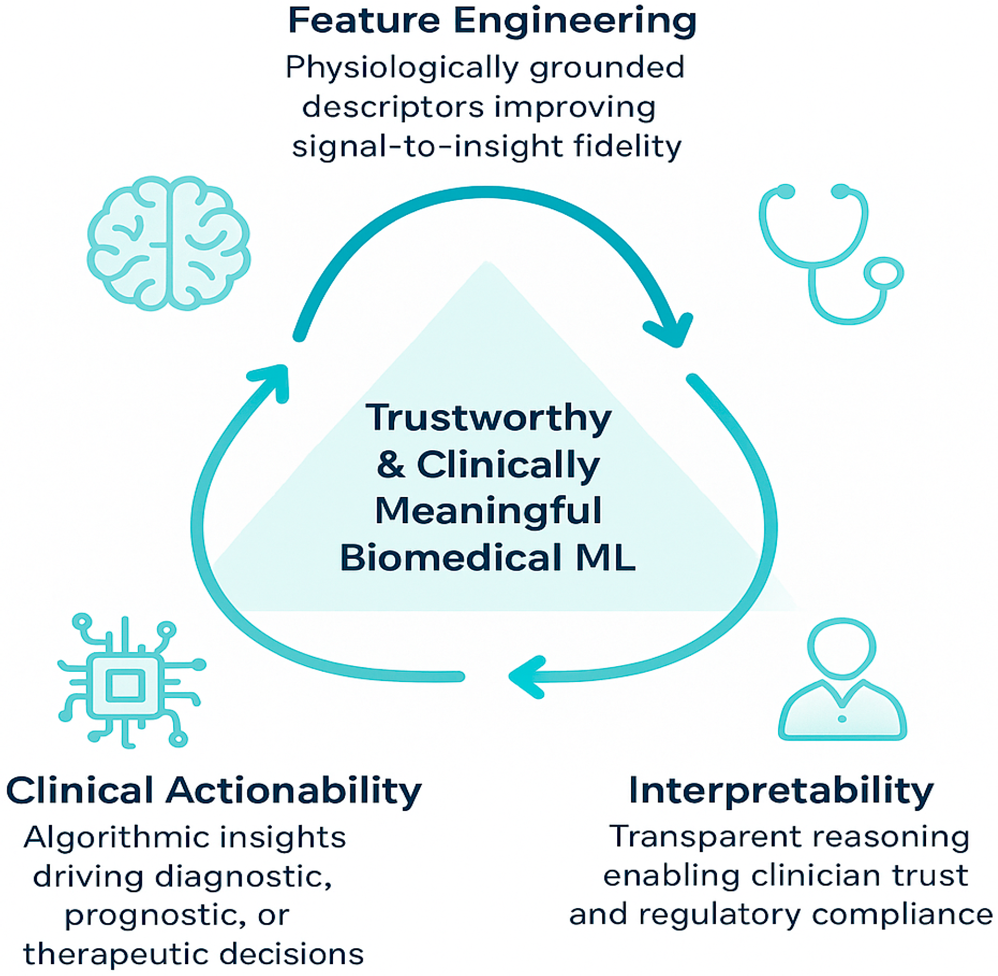
Figure 1. Conceptual framework linking feature engineering, interpretability, and clinical actionability in biomedical machine learning.
Applsci 15 12036 g001
Figure 2. Flowchart of the multistage screening process for selecting relevant studies. This diagram outlines the steps from initial record identification to the final selection of included studies.
Applsci 15 12036 g002
Figure 3. Graphical representation of the keywords covered in this review.
Applsci 15 12036 g003
Figure 4. The number of publications with citations over the years.
Applsci 15 12036 g004
Figure 5. The number of publications per journal.
Applsci 15 12036 g005
Figure 6. The flowchart for choosing between DL, ML, and hybrid.
Applsci 15 12036 g006
Figure 7. Performance of ML vs. DL on Biomedical Signals vs. Dataset size.
Applsci 15 12036 g007
Figure 8. A conceptual diagram illustrates the process of extracting features from raw biomedical signals into time-domain, frequency-domain, and time-frequency-domain features.
Applsci 15 12036 g008
Figure 9. Time, frequency, and time–frequency domain representations of an ECG signal segment. (a) Raw ECG waveform highlighting the QRS complex (red marker) and a transient artifact (green marker). (b) Frequency domain representation (FFT magnitude spectrum). (c) Power spectral density (PSD) with shaded regions indicating physiologically relevant frequency bands. (d) Spectrogram showing time-varying frequency content with vertical annotations marking the QRS complex and artifact events.
Applsci 15 12036 g009
Figure 10. A Conceptual diagram illustrates the three main categories of feature selection methods and their relationship to machine learning models.
Applsci 15 12036 g010
Figure 11. Sample features selection (importance) using random forests.
Applsci 15 12036 g011
Figure 12. Comparison of machine learning classifiers based on key performance metrics including accuracy, sensitivity, specificity, and AUC. Overall, ensemble-based methods such as CatBoost, AdaBoost, and Random Forest demonstrated superior performance across most metrics. CatBoost achieved the highest specificity and AUC, indicating excellent discriminative ability, while AdaBoost and Random Forest showed the best sensitivity, reflecting strong detection of positive cases. Simpler models like Naïve Bayes and SVM yielded comparatively lower scores across all metrics. These results suggest that ensemble approaches provide more balanced and robust performance for this classification task.
Applsci 15 12036 g012
Figure 13. Flow chart of subject-independent and external testing.
Applsci 15 12036 g013
Figure 14. Visualization of six-dimensional reduction and feature projection techniques applied to biomedical data. Each subplot displays the two-dimensional projection of a high-dimensional feature space. Linear methods (PCA, ICA, LDA) are compared with non-linear and deep learning-based methods (t-SNE, UMAP, and Autoencoder). The color scale represents the two classes in the dataset.
Applsci 15 12036 g014
Figure 15. Conceptual diagram illustrating methods for interpreting traditional machine learning models, showing both model-specific and post hoc approaches.
Applsci 15 12036 g015
Figure 16. Sample Feature Importance Plot.
Applsci 15 12036 g016
Figure 17. Sample Partial dependence plot.
Applsci 15 12036 g017
Figure 18. Sample ICE plot.
Applsci 15 12036 g018
Figure 19. SHAP values sample plot.
Applsci 15 12036 g019
Figure 20. Sample LIME features plot.
Applsci 15 12036 g020
Figure 21. Conceptual illustration linking feature engineering to clinical interpretation. Each feature domain provides distinct physiological insights, which machine learning models subsequently interpret to support clinical decision-making.
Applsci 15 12036 g021
Figure 22. Standard performance metrics for evaluating machine learning classification models in biomedical signal analysis.
Applsci 15 12036 g022
Figure 23. Variance of sensitivity and specificity across ML models.
Applsci 15 12036 g023
Figure 24. Common setup for processing TBSs.
Applsci 15 12036 g024
Figure 25. PSD of two breathing sounds from Non-OSA and OSA TBS.
Applsci 15 12036 g025
Figure 26. PSD, STFT, and MFCC characterization of Non-OSA TBS.
Applsci 15 12036 g026
Figure 27. Main Challenges and Limitations of ML for Biomedical Signals.
Applsci 15 12036 g027
Figure 28. Accuracy and model interpretability tradeoff.
Applsci 15 12036 g028
Figure 29. The flow diagram of ML-DL hybrid Models.
Applsci 15 12036 g029
Figure 30. The federated learning block diagram.
Applsci 15 12036 g030
Figure 31. Schematic of multi-modal biomedical signal integration. Raw signals (e.g., ECG, EEG, TBS) are preprocessed, features are extracted, and either concatenated (feature-level fusion) or combined after separate classifiers (decision-level fusion), resulting in improved diagnostic or monitoring performance.
Applsci 15 12036 g031
Table 1. Comparison of Traditional ML and Deep Learning for Biomedical Signals.
FactorMachine LearningDeep LearningImplication for Medical Use
InterpretabilityHigh (Decision rules, feature importance)Low (“Black-box” nature)Traditional ML is preferred for clinical trust and validation.
Data RequirementsLow to ModerateVery HighTraditional ML is often the only viable option for most specific medical studies.
Computational CostLow (runs on CPU)High (requires GPUs)Traditional ML enables real-time analysis on low-power devices.
Domain KnowledgeExplicitly incorporated via feature engineeringLearned implicitly from dataTraditional ML leverages and validate existing clinical expertise.
Regulatory Pathsimpler, more transparentcomplex, requires extensive validationTraditional ML is better aligned with current medical device approval frameworks.
Table 2. Comparative performance of ML and DL models for biomedical signal analysis, highlighting accuracy across dataset sizes, interpretability, computational cost, and alignment with clinical requirements.
FactorMLDLImplication for Biomedical Signals
Accuracy (small data)85–92% (n < 2000)70–85% (n < 2000)ML preferred for small datasets
Accuracy (large data)90–93% (n > 10,000)92–98% (n > 10,000)DL surpasses ML only with large datasets
InterpretabilityHigh (decision rules, feature importance)Low (“black-box”)ML favored for clinical trust and validation
Computational costLow (CPU, minutes)High (GPU, hours)ML enables real-time deployment
Feature engineeringExplicit, domain-informedImplicit, learned from dataML leverages existing clinical knowledge
Table 3. Gap Analysis of Traditional ML and DL Approaches for Biomedical Signal Analysis.
ModalityMethodMetricInterpretabilityClinical ValidationGap Identified
ECGSVM, RF, DTAccuracy, F1HighPartialLimited benchmarking across small vs. large datasets
EEGSVM, CNN, LSTMAccuracy, AUCMediumLimitedInterpretability for complex DL models lacking
EMGRF, RNNAccuracyHighPartialInconsistent validation across heterogeneous populations
Tracheal SoundsSVM, RF, DTSpecificity, SensitivityHighRareFew studies include clinical outcome validation
EVestGML, DL hybridsAccuracy, SensitivityMediumLimitedSparse comparative studies and hybrid model evaluation
PPGML, CNNAccuracy, F1MediumPartialLimited transparency and reproducibility reporting
Table 4. Common Time-Domain Features for Biomedical Signal Analysis. This table provides examples, descriptions, and typical applications of amplitude-based, morphological, and statistical features extracted directly from the signal waveform.
Feature CategoryExamplesDescriptionsApplication in Biomedical Signals
Amplitude-basedMax, Min, Mean, RMS, Variance, Std DevQuantify signal amplitude and powerEMG (RMS for muscle activity), TBS (RMS for breathing intensity)
MorphologicalP-wave duration, QRS complex duration, ST-segment elevationDescribe the shape of specific signal componentsECG (diagnosing cardiac conditions), EMG (WAMP for muscle activity)
StatisticalSkewness, Kurtosis, Zero-crossing rateDescribe the distribution and periodicity of the signalRespiratory sounds (ZCR for frequency content)
Table 5. Standard Frequency and Time-Frequency Domains Features for Biomedical Signal Analysis.
Feature CategoryExamplesDescriptionApplication in biomedical Signals
Spectral ContentPower Spectral Density (PSD), Spectral Centroid, Band Power RatiosQuantify the distribution of power across frequenciesEEG (alpha, beta, theta, delta bands), HRV from ECG, Respiratory sounds (wheezes, crackles)
Speech-relatedMel-Frequency Cepstral Coefficients (MFCCs)Capture spectral envelope, robust to recording variationsTracheal breathing sounds (robust representation of respiratory sounds)
Wavelet Transform (WT)Decomposes the signal into different frequency components at various resolutions.ECG, EEG (capturing transient and oscillatory phenomena)Wavelet Transform (WT)
Short-Time Fourier Transform (STFT)Provides a spectrogram, a visual representation of frequency content over timeEvoked potentials in EEG, transient events in ECG (changes in power or dominant frequencies)Short-Time Fourier Transform (STFT)
Table 6. Comparison of Feature Selection Methods. This table provides an overview of filter, wrapper, and embedded feature selection techniques, detailing their advantages and disadvantages.
Method TypeDescriptionAdvantagesDisadvantagesExamples
Filter MethodsSelect features based on intrinsic properties, independent of the ML modelComputationally efficient, suitable for high-dimensional dataIgnore interaction with ML model, may select redundant featuresVariance Threshold, Correlation-based Feature Selection (CFS), Statistical Tests (Chi-squared, ANOVA, Mutual Information)
Wrapper MethodsEvaluate feature subsets by training and testing an ML modelConsider interaction with the ML model, which is generally more accurateComputationally expensive, prone to overfitting with small datasetsForward Selection, Backward Elimination, Recursive Feature Elimination (RFE)
Embedded MethodsPerform feature selection during model trainingBalance of efficiency and accuracy, considers feature interactionsMethod-dependent, less flexible than filter methodsLasso (L1 Regularization), Tree-based Methods (Decision Trees, Random Forests, Gradient Boosting)
Table 7. Comparison of Traditional Machine Learning Algorithms for Biomedical Signal Analysis. This table summarizes the characteristics, strengths, weaknesses, and typical applications of various traditional ML models.
AlgorithmStrengthsWeaknessesApplications in Biomedical Signals
Logistic RegressionSimple, interpretable, and effective for linear relationshipsAssumes linearity, poor for complex non-linear dataBinary classification (e.g., disease presence/absence, respiratory sound classification)
Linear Discriminant Analysis (LDA)Interpretable, effective for class separabilityAssumes normal distribution and equal covarianceEEG (emotion recognition), ECG (classification), BCI systems, EVestG
PerceptronFast and straightforward, foundational to neural networksLimited to linearly separable problemsECG (beat classification), breathing pattern analysis
Naïve BayesFast, efficient with high-dimensional dataAssumes feature independenceReal-time biomedical monitoring, initial classification
Support Vector Machines (SVMs)Robust to overfitting, works well with high-dimensional dataSensitive to kernel choice and noisy dataECG (arrhythmia), EEG (seizure detection), EMG (movement recognition), respiratory sounds, EVestG
K-Nearest Neighbors (KNN)Simple, non-parametric, easy to interpretComputationally expensive, sensitive to irrelevant featuresECG (heartbeat classification), EEG (sleep stages), respiratory sound analysis
Decision TreeHighly interpretable, handles mixed data typesProne to overfitting, unstable to small data changesDisease diagnosis, respiratory pathology identification
Random ForestRobust, accurate, handles high-dimensional dataLess interpretable (ensemble nature)Sleep stage classification, disease diagnosis
AdaBoostHigh accuracy, focuses on difficult casesSensitive to noise and outliersSleep stage detection, respiratory sound pathology
CatBoostExcellent with categorical features, less overfittingComputationally intensiveMultimodal disease prediction, respiratory sound analysis
Artificial Neural Networks (Shallow)Models complex, non-linear patternsRequires more data, less interpretableGeneral biomedical classification tasks
Logistic RegressionSimple, interpretable, and effective for linear relationshipsAssumes linearity, poor for complex non-linear dataBinary classification (e.g., disease presence/absence, respiratory sound classification)
Table 8. Comparative overview of common XAI methods used in biomedical signal analysis, summarizing their methodological type, key strengths, limitations, and representative clinical applications.
MethodTypeStrengthsLimitationsRepresentative Clinical Example
SHAPGlobal & LocalQuantitative feature attribution; consistent with game-theoretic fairnessComputationally intensive; may yield unstable results for correlated featuresEEG seizure biomarkers; heart-sound murmur detection
LIMELocalExplains individual predictions; model-agnostic; intuitive for cliniciansSensitive to perturbation sampling; limited reproducibilityRespiratory sound interpretation; ECG anomaly explanation
Permutation ImportanceGlobalSimple to compute; directly comparable across modelsMay ignore feature interactionsFeature relevance in sleep apnea detection
Partial Dependence/ICE PlotsGlobal/LocalVisualizes marginal and individual feature effectsAssumes feature independence; can obscure nonlinearitiesRelation between spectral centroid and breathing abnormality
Model-Specific (Tree/Linear Models)IntrinsicDirectly interpretable through weights or rules; low computational costLimited flexibility for non-linear or high-dimensional dataLogistic regression for OSA risk prediction; rule-based decision trees for cough classification
Table 9. Clinical Relevance of Common Feature Types Across Biomedical Signals.
Feature DomainExample FeaturesPhysiological/Clinical RelevanceTypical Applications
Time-DomainRMS, Mean, Zero-Crossing Rate, P-wave duration, QRS widthReflects amplitude, rhythm, and morphology of physiological eventsECG arrhythmia detection, EMG muscle activation, TBS airflow intensity
Frequency-DomainPSD, Spectral Centroid, Band Power Ratios, MFCCsQuantifies oscillatory patterns and energy distributionEEG (brain waves), respiratory sound wheeze/crackle detection, HRV analysis
Time–Frequency DomainWavelet Energy, STFT features, Spectrogram statisticsCaptures transient or non-stationary physiological changesEEG evoked potentials, TBS phase differentiation
Non-Linear FeaturesEntropy, Fractal Dimension, Lyapunov ExponentIndicates signal complexity and regulatory balanceEEG seizure detection, ECG variability, cognitive state assessment
Higher-Order StatisticsBispectrum, Trispectrum, Skewness, KurtosisDetects non-Gaussianity and coupling of physiological eventsEEG cross-frequency coupling, respiratory anomaly analysis
Table 10. Linking Model-Derived Feature Importance to Clinical Interpretation.
ML ModelInterpretability OutputClinically Meaningful InsightExample in Practice
Decision TreeExplicit decision rules (e.g., “if RMS > 0.5→abnormal”)Transparent condition–decision mappingRespiratory sound classification (standard vs. abnormal)
Random ForestFeature importance rankingIdentifies dominant physiological markersEEG: α/β ratio importance in drowsiness detection
Logistic RegressionFeature coefficients (positive/negative weights)Quantifications of the direction of clinical associationECG: prolonged QRS duration positively linked to arrhythmia risk
SVMSupport vector influenceHighlights boundary-defining physiological patternsEMG: separation between rest and contraction epochs
SHAP/LIME (Post hoc)Local feature contribution per instanceCase-by-case interpretability of prediction rationaleTBS: spectral centroid and RMS jointly drive OSA classification
Table 11. Key Performance Metrics for Evaluating Machine Learning Models in Biomedical Applications. This table defines and compares various metrics for assessing the performance of classification and regression models.
MetricDescriptionImportance of Biomedical Signals
AccuracyProportion of correctly classified instancesCan be misleading with class imbalance; general overview
PrecisionTrue positives among all optimistic predictionsCrucial when false positives are costly (e.g., unnecessary procedures)
Recall (Sensitivity)True positives among all actual positive instancesCritical when false negatives are costly (e.g., missing a diagnosis)
F1-ScoreHarmonic mean of precision and recallBalanced measure, useful with uneven class distributions
SpecificityTrue negatives among all actual negative instancesEssential for avoiding false alarms
AUC-ROCArea under the Receiver Operating Characteristic curveRobust measure of classifier performance, independent of threshold
Table 12. Representative quantitative comparison of traditional ML vs. DL performance across biomedical signal modalities.
SignalDatasetML (Best)DL (Best)MetricReference
EEGTUH EEGSVM (0.93 ± 0.02)CNN (0.96 ± 0.04)AUC[24,67,127]
ECGMIT-BIHRandom Forest (0.94 ± 0.03)1-D CNN (0.91 ± 0.05)F1[66,128]
EMGNinaproSVM (0.89 ± 0.04)RNN (0.92 ± 0.06)Accuracy[24]
TBSAwakeOSARandom Forest (0.82)CNN (0.73)Specificity[126,129]
Table 13. Tracheal Breathing Sound (TBS) Analysis Case Study Summary.
StepMethod/FeaturesNotes/Performance
Signal AcquisitionMicrophone at suprasternal notch; band-pass filter (75–3000 Hz)Reduces low-frequency body noise, high-frequency artifacts
PreprocessingSegmentation of breath cycles; normalizationEnsures consistency across subjects
Time-Domain FeaturesRMS, ZCR, Peak Amplitude, Breath Duration, Breath RateCorrelated with airflow intensity and obstruction
Frequency FeaturesPSD in (100–250 Hz) and (300–500 Hz) bands; CentroidDetects turbulence and abnormal airflow patterns
Time–FrequencySTFT spectrogram features; Wavelet coefficientsCaptures transient events and non-stationary components
Classifiers TestedSVM (83.92% testing accuracy), Random Forests (81.4% testing accuracy), Regularized logistic regression (79.3% ± 6.1% testing accuracy)SVM and RF show the best accuracy; Trees are the most interpretable
Table 14. Challenges and Potential Solutions in Traditional ML for Biomedical Signals.
ChallengeDescriptionPotential Solutions
Noise and ArtifactsMotion artifacts, electrode noise, and environmental interferenceFiltering, ICA, adaptive preprocessing, wavelet denoising
Non-StationarityPhysiological signals vary dynamically over timeTime–frequency features, wavelets, adaptive feature extraction
ScalabilityManual feature engineering and some algorithms scale poorly with large datasets.Automated feature selection, ensemble methods, dimensionality reduction (PCA/ICA)
Interpretability vs. AccuracyTrade-off between transparent models and high-performance ensemblesHybrid models, post hoc interpretability (SHAP, LIME), feature importance visualization
Temporal DependenciesDifficulty capturing long-term dynamicsWindow-based features, sequence models integrated with traditional ML
Table 15. Table listing and comparing major open-source biomedical signal toolboxes, their features, and target signals.
ToolboxSupported SignalsKey Features
BioSPPyECG, PPG, EMG, resp.Time, frequency, time-frequency, denoising
NeuroKit2EEG, ECG, EDAEntropy, fractal, HRV, ML ready
PyWaveletsAllCustomizable wavelet transforms
Table 16. Representative ML Performance for Selected Biomedical Signal Benchmarks.
DatasetTask/SignalBest AlgorithmAccuracy (%)Sensitivity (%)Specificity (%)
MIT-BIH ArrhythmiaECG classificationSVM, Random Forest97–999698
PhysioNet Sleep-EDFSleep staging/EEGRandom Forest88–928691
Respiratory Sound DBWheeze/CrackleRandom Forest, DT93–969094
Disclaimer/Publisher’s Note: The statements, opinions and data contained in all publications are solely those of the individual author(s) and contributor(s) and not of MDPI and/or the editor(s). MDPI and/or the editor(s) disclaim responsibility for any injury to people or property resulting from any ideas, methods, instructions or products referred to in the content.