Article

Neural Modelling of CO2 Emissions from a Selected Vehicle

by
Magdalena Rykała
Faculty of Security, Logistics and Management, Military University of Technology, 00-908 Warsaw, Poland
Appl. Sci. 2025, 15(22), 12037; https://doi.org/10.3390/app152212037
Submission received: 20 October 2025 / Revised: 6 November 2025 / Accepted: 9 November 2025 / Published: 12 November 2025
(This article belongs to the Section Transportation and Future Mobility)

Abstract

The article addresses the problem of modelling instantaneous CO2 emissions from a specific motor vehicle equipped with an internal combustion engine. The article’s concept is based on a review of current research, which led to the identification of a list of variables essential to constructing the numerical model. Data was collected through recording selected vehicle parameters during test drives using the OBD diagnostic interface. The article describes the model development process and presents the results of CO2 emission modelling using MLP neural networks. The performance of various architectures was examined, considering the number of hidden layers (1, 2, 3), the number of neurons in each layer (from 10 to 267), and different activation functions (such as sigmoid, hyperbolic tangent, and ReLU). Consistency in the values of the MSE, RMSE, and MAE indicators during both validation and testing phases demonstrates the accuracy of the models. High R2 values of around 0.8 confirm that MLP networks can effectively model CO2 emissions from motor vehicles.

1. Introduction

CO2 emissions modelling has become a rapidly growing area of research with significant implications for the environment. The modelling process yields a model that predicts emissions based on a range of parameters. In the macroscopic approach [1], emission values are determined using available information about the vehicle fleet, such as traffic intensity, traffic speed, and load, based on the number and type of vehicles. Companies use these methods to optimise CO2 emissions. For individual vehicles, microscopic (instantaneous) models that determine instantaneous emission rates for each vehicle are used [2,3]. This approach, in turn, allows for the optimisation of CO2 emissions at the level of the ordinary traffic user [4].
Several methods are used for the mathematical modelling of CO2 emissions. In addition to mathematical models based on linear regression [5], more complex and modern methods are increasingly being used [6], such as decision trees [7], fuzzy logic [8], neural networks [9,10], deep learning [11], etc. In article [11], deep learning algorithms (LSTM recurrent networks) were used to build a model of CO2 emissions from passenger cars. Data for the model was collected in real time from the vehicle’s OBD (On-Board Diagnostics) interface. In turn, article [9] developed a neural network-based model of NOₓ and CO2 emissions from motor vehicles using data from a portable emissions measurement system (PEMS). Recent trends in vehicle CO2 modeling clearly point to the use of increasingly advanced artificial intelligence methodologies, employing both data-driven approaches and deep learning architectures, which show great potential for predicting vehicle emissions with high accuracy while integrating explainable artificial intelligence (XAI) techniques [12]. Neural network models that incorporate the laws of physics are another promising direction, incorporating domain-specific dependencies to improve problem generalization, especially for real-world driving scenarios [13]. Machine learning models are also a widespread solution in this context [14]. Machine learning ensemble methods, including Random Forest, XGBoost, CatBoost, and LightGBM, are effective alternatives to neural networks. Their use in modeling CO2 emissions from vehicles outperforms traditional linear approaches while maintaining computational efficiency [15]. Hybrid approaches combining several types of neural networks are also becoming increasingly common, e.g., the CNN-LSTM-MLP [7], which combines a recurrent network (LSTM), a convolutional neural network (CNN), and a multilayer perceptron (MLP). Deep learning-based neural networks achieve high R2 values, but this comes at the cost of long training times and enormous computing resources [16].
CO2 emissions from motor vehicles are directly related to fuel combustion in internal combustion engines. Article [17] reports a correlation coefficient of approximately 0.999 between CO2 emissions and fuel consumption, indicating a linear relationship between the two variables. Therefore, it has been established that burning 1 litre of diesel fuel in a diesel engine generates approximately 2.68 kg of CO2, while burning 1 litre of gasoline generates approximately 2.3 kg of CO2.
Another significant issue is measuring CO2 emissions. Article [18] evaluates the observed differences between actual CO2 emissions and those measured under laboratory conditions. The level of greenhouse gas emissions, including CO2, can be measured using the PEMS system, which has been the subject of many scientific articles, e.g., [19,20,21].
The driver can also significantly impact CO2 emissions [22]. The connection between his behaviour on the road and the vehicle’s dynamics is also the subject of research [23]. An OBD interface is often used to access dynamic vehicle parameters, such as engine speed, vehicle speed, load, and throttle position [5]. Of the factors mentioned, vehicle acceleration has a significant impact on CO2 emissions [24,25]. Furthermore, due to limitations in specific parameters, e.g., vehicle speed or acceleration, other time-based positioning systems are often used for this purpose, such as GNSS (Global Navigation Satellite Systems) [26], Ultra-Wideband [27], or IMU (Inertial Measurement Unit) [28].
In summary, the literature review showed that neural networks can effectively model complex relationships between various variables, including vehicle speed, instantaneous engine parameters, and instantaneous CO2 emissions. In turn, OBD diagnostic interfaces, coupled with other sensors or mobile devices, e.g., smartphones, are most commonly used to collect the aforementioned data. This study aims to develop and validate a neural network model capable of predicting instantaneous CO2 emissions from combustion vehicles under real-world operating conditions, using real-time data from the OBD interface. A key element of the study is the identification and selection of key input variables that significantly determine CO2 emissions. Proper parameter selection reduces data redundancy and improves model learning efficiency, thus increasing its generalizability. The result is a tool that enables not only quantitative, real-time emissions assessment but also qualitative analysis of the impact of individual operational factors, providing a foundation for practical application in monitoring and optimizing eco-driving.
This also highlights the study’s innovative nature, which combines two perspectives. It demonstrates the potential of using available OBD data, and it emphasizes the importance of systematically selecting key factors that determine CO2 emissions and integrating them into an artificial neural network model.
Previous research typically focuses on laboratory emission measurements, which are expensive and difficult to access, or on general operational indicators that overlook the dynamic and complex interdependencies among engine operating parameters. However, the proposed solution introduces a new perspective by using only diagnostic variables available to every vehicle user. Therefore, the article not only makes a scientific contribution by providing a mathematical model for identifying CO2 emissions, but also has significant practical implications and application potential.

2. Materials and Methods

Measuring CO2 emissions is a complex process and can be done in various ways. The most accurate measurement methods involve the use of PEMS, which is the most common method of CO2 emission measurement in laboratory conditions [20,21,22,29], etc. These sensors can also be used in real-world situations, but due to the large dimensions of this type of device, their installation at the rear of the vehicle is usually problematic. Therefore, the OBD diagnostic interface was used in the tests to determine CO2 emissions. This approach provided access to a range of parameters directly related to engine operation. To record data from the above-mentioned interface, a smartphone equipped with a GNSS chip was used, connected wirelessly to the OBD interface via Wi-Fi. The presented study is grounded in a locally coordinated experimental program affiliated with the Military University of Technology.

2.1. Research Methodology

Based on the CO2 emissions analysis, a set of parameters was selected to construct a CO2 emissions model for motor vehicles. Due to the large number of variables involved, additional criteria were adopted that the parameters must meet. Firstly, technical parameters of the vehicle over which the driver has no direct influence, such as dimensions, weight, engine displacement, and others (dependence criterion), were omitted. In addition, it was assumed that the parameters must be readable from the OBD interface or a mobile phone (measurement accessibility criterion). Among the parameters that can be calculated indirectly, i.e., based on other parameters, vehicle acceleration was selected. Ultimately, based on the accepted criteria, the following parameters were selected:
  • engine speed,
  • engine load,
  • vehicle speed,
  • vehicle acceleration,
  • throttle position,
  • altitude,
  • CO2 emissions.
To obtain the experimental data needed to construct CO2 emission models, a series of test drives was conducted with a selected car. The experimental research involved recording selected parameters of a moving motor vehicle. For this purpose, a Mazda 3 car with a spark-ignition engine was selected (Table 1). The choice of a single vehicle was based on practical considerations such as accessibility and convenience. Limiting the study to a single car allowed for the elimination of variability resulting from design differences (weight, power, drivetrain). The Mazda 3 (Mazda Motor Corporation, Fuchu, Japan) is one of the available and popular models on the European market, and in a sense, it can be treated as a representation of a typical car in Europe. The study area was Poland, and it was decided to record short sections of the routes, which were chosen to be as diverse as possible. The routes included many urban sections and frequent stops (engine on/off), which allowed for recording the vehicle’s different driving modes.
The recorded parameters, along with their descriptions and classification as input or output variables, are presented in Table 2.
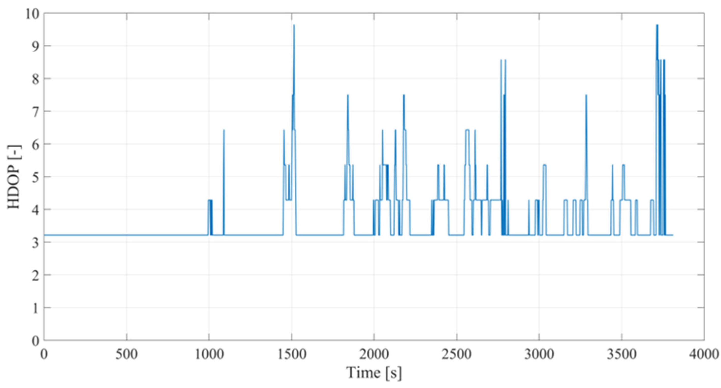
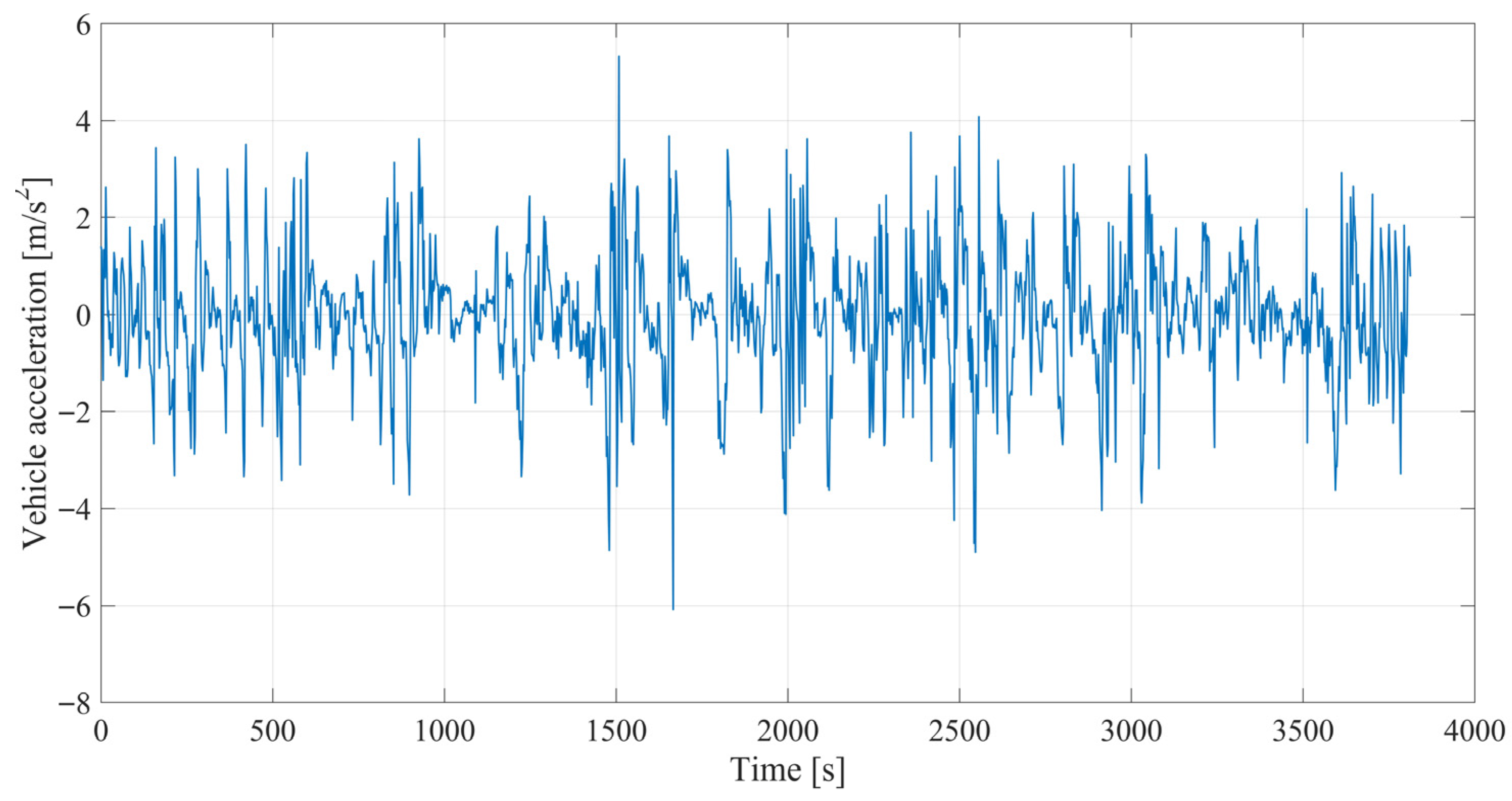
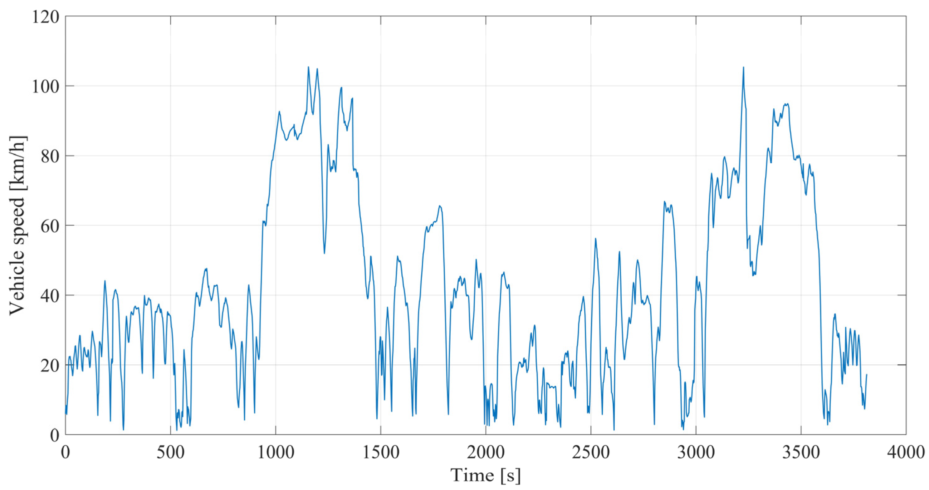
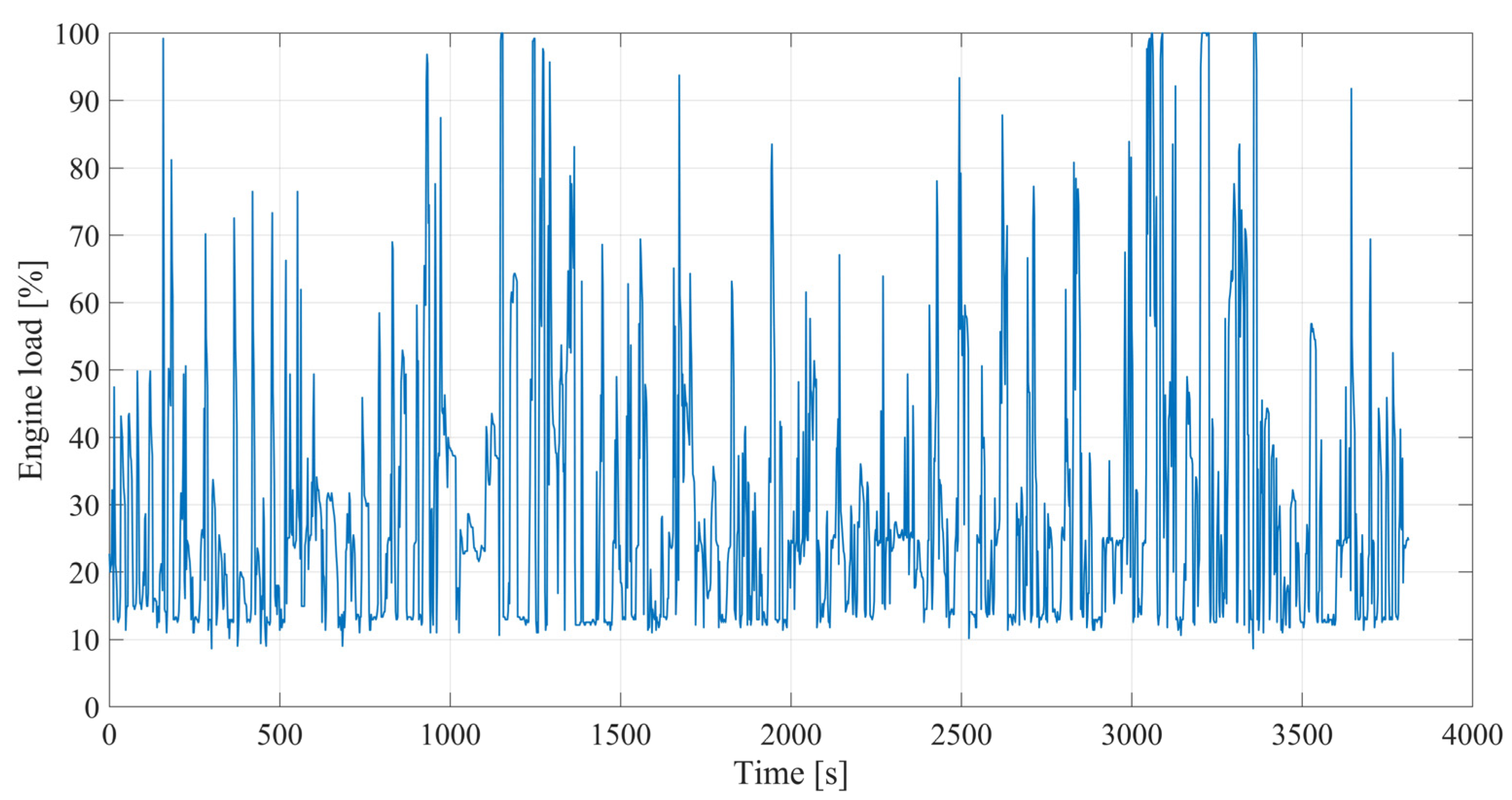
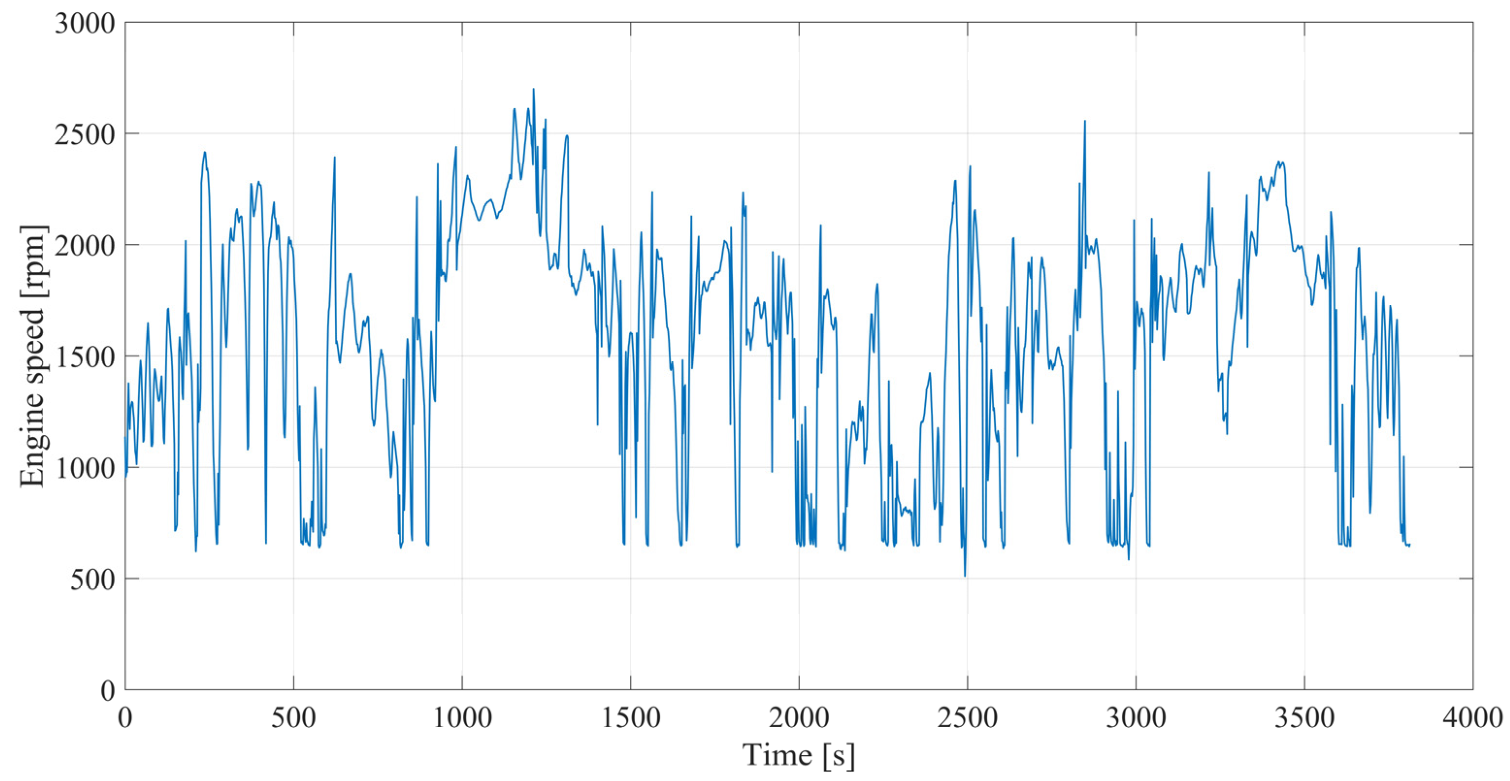
An OBD Vgate iCar Pro (Vgate, Shenzhen, China) adapter was used to record vehicle data. Parameters such as vehicle speed and altitude were recorded using the mobile phone’s built-in GNSS receiver (Torque Pro app, Android; ver. 1.12.101; Ian Hawkins, Newport Pagnell, Buckinghamshire, UK). Vehicle acceleration was determined based on vehicle speed measurements. To minimize the influence of outliers on the measurement results, the data were pre-filtered using the percentile method with an upper bound of the 95th percentile. Furthermore, since it is not possible to determine CO2 emissions during operation when the vehicle is stationary, these observations and idling were not taken into account. No missing data were observed in the recorded waveforms. Furthermore, no signal filtering was used to avoid introducing distortions that could affect subsequent measurement analysis. This approach ensures the universality of the method and preserves the original signal properties. The omission of pre-filtering also enables direct comparison of results with other raw measurement data. To evaluate the performance of the GNSS system on the mobile phone, the HDOP (Horizontal Dilution of Precision, Figure A1) and the number of satellites (Figure A2) were also recorded during the measurements (Appendix A). Figure 1, Figure 2, Figure 3, Figure 4, Figure 5, Figure 6 and Figure 7 show graphs of recorded variables, namely altitude above sea level, vehicle acceleration, vehicle speed, engine load, engine speed, throttle position, and CO2 emissions.
Table 3 presents the basic statistics of the described variables.
Then, the correlation values between the independent variables and the dependent variable were determined (Table 4).
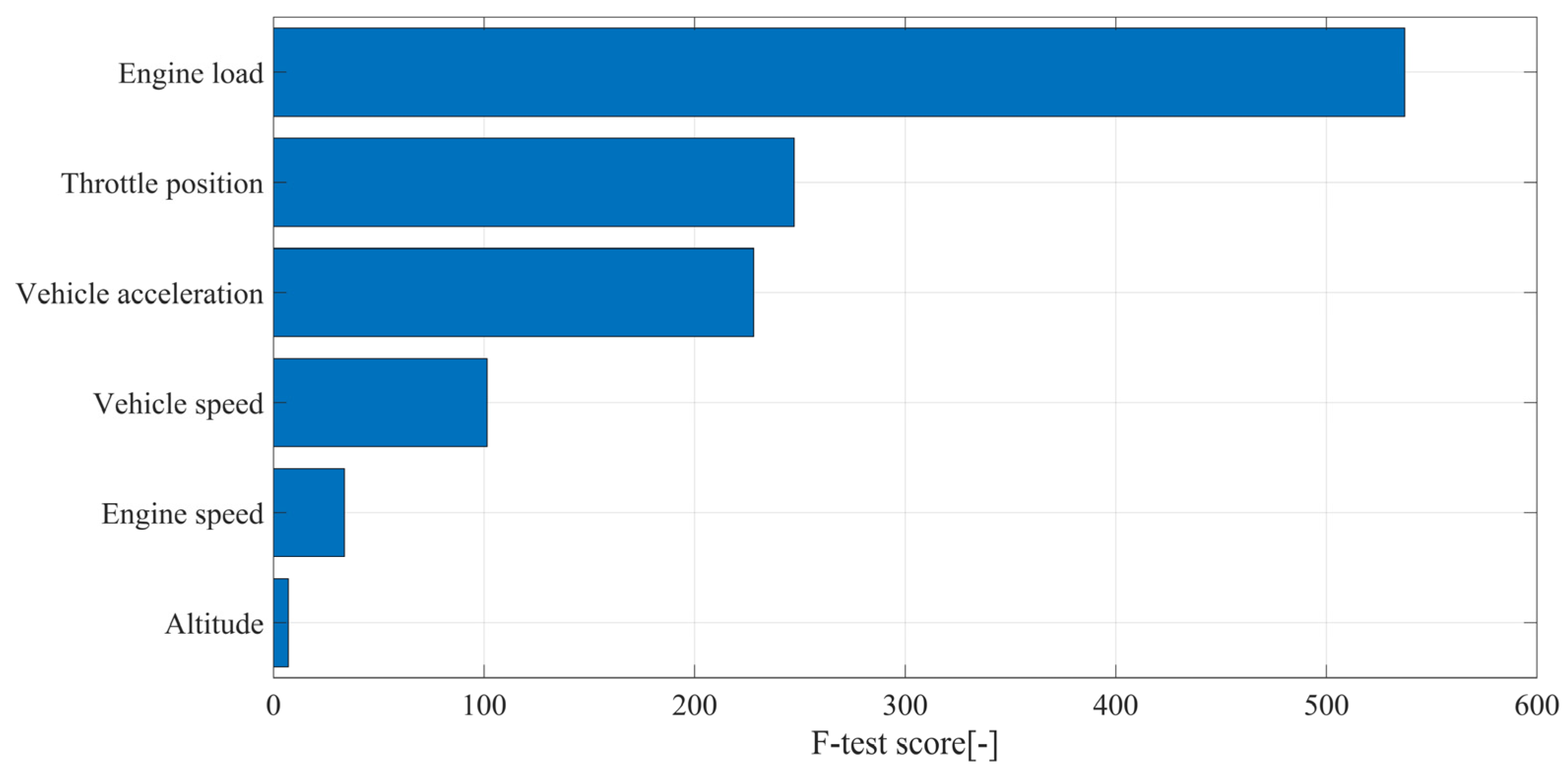
The presented correlation values for the altitude and engine speed variables are low, suggesting a lack of a linear relationship between these variables and the output variable. Given the values as mentioned above, the model variables were selected using feature selection methods, including the F-test, which specifies a limited number of variables with the highest F-scores (Figure 8) [30].
The F-test tests the hypothesis that response values grouped by predictor values come from a population with the same mean, compared to the hypothesis that the population means differ [31]. The variables with the highest values are engine load, throttle position, vehicle acceleration, and vehicle speed. The variables with the lowest values are Engine speed and altitude.
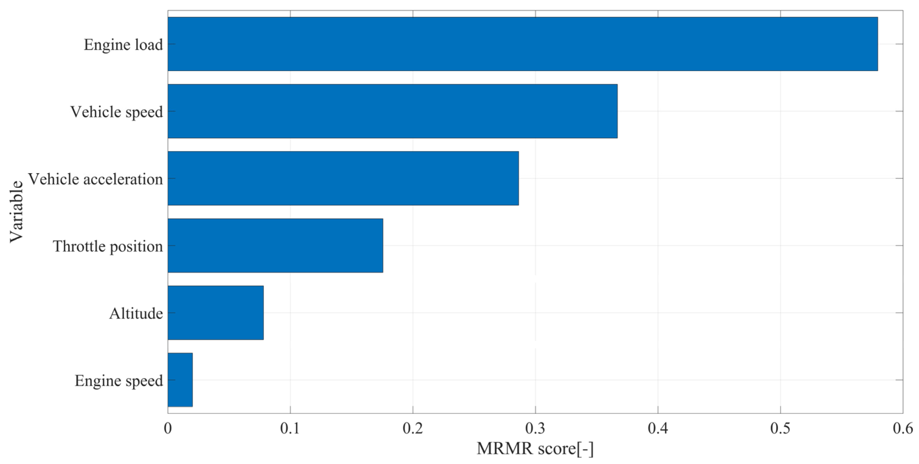
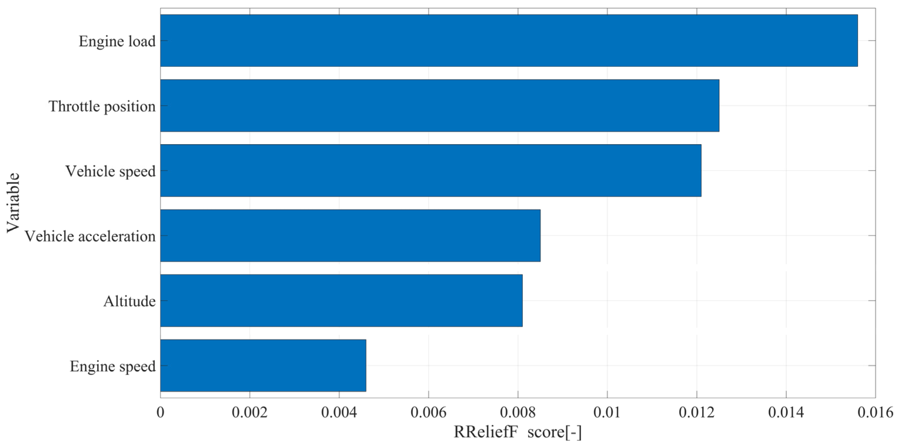
Then, the scores of the MRMR (Minimum Redundancy Maximum Relevance) and RreliefF algorithms were determined. RReliefF is a regression-based algorithm detecting interactions between variables and non-linear dependencies through nearest-neighbor analysis. In turn, MRMR identifies variables with the strongest relationships to the target variable while minimizing redundancy among the selected variables [31].
All of the above methods (Figure 8, Figure 9 and Figure 10) confirmed negligible importance scores for two variables: engine speed and altitude. Ultimately, these two variables were rejected in the later part of the model development. All calculations presented in the article were performed in MATLAB R2023b software.

2.2. Modelling Methods

Several types of neural networks differ in their architectures and applications. The most important of them include CNN and LSTM networks used in image and text processing. In cases of modelling nonlinear systems, especially with simpler databases, MLP networks are used, consisting of several layers of neurons. The most important parameter of this type of network is the so-called number of hidden layers. The following relations can simplify the architecture of MLP neural networks with three hidden layers:
y = f 4   W ( 4 ) f 3 W ( 3 ) f 2 W ( 2 ) f 1 W ( 1 ) x + b 1 + b 2 + b 3 + b 4
where
  • x—input vector,
  • W(i)—weight matrices of the i-th layer,
  • b(i)—threshold value of the i-th layer,
  • f(i)—activation function of the i-th layer,
  • y—output vector [32].
The number of hidden layers influences the network’s complexity, significantly increasing its capacity to store information (the number of weights in the layers). However, MLP networks with one or two hidden layers are most often used. Each layer has a certain number of neurons. The number of input and output neurons is determined by a given data set; thus, for example, a 10-5-5-5-1 MLP network consists of ten input neurons, three hidden layers with five neurons each, and one output neuron. This also means that the network has 10 input signals (vector x) and one output signal (vector y) [33].
The links between the layers of neural networks are the activation function. The most commonly used activation functions include sigmoid function, hyperbolic tangent, and ReLU (Rectified Linear Unit). The sigmoid function can be described by the following relationship:
φ ( x ) = 1 1 + e x
The range of sigmoid functions is (0, 1), while a typical example is the logistic function. Due to the features mentioned above, it is particularly applicable to datasets involving probability or binary problems [32,33].
In turn, the hyperbolic tangent can be written as follows:
t a n h ( x ) = e x e x e x + e x
This function is bipolar, i.e., it takes values in the range (−1, 1), but near zero it has a linear character, which facilitates the learning process [32,33].
The last function mentioned is ReLU, and one way to represent it is the following relation:
R e L U ( x ) = x + x 2
ReLU is a function often used to speed up computations due to its straightforward relationship used in networks with more than two hidden layers [32,33].
The goal of using neural networks is to build a model that most accurately reflects a given data set. This is possible using neural network training algorithms. One of the most commonly used algorithms for training neural networks is the BFGS (Broyden-Fletcher-Goldfarb-Shanno) algorithm, which belongs to the group of iterative non-linear optimisation algorithms [34].
The most commonly used metrics for evaluating neural network models include: MSE (Mean Squared Error), RMSE (Root Mean Squared Error), MAE (Mean Absolute Error), and R2. These indicators allow the assessment of model prediction errors, which is crucial for finding a model that most accurately reflects the input data [34,35].
The MSE indicator is the value of the mean sum of squares of the difference between the predicted and actual values.
M S E = i = 1 n y i y ^ i 2 n
where
  • n—the number of observations,
  • y i —the i-th observed (actual) value,
  • y ^ i —the i-th predicted value [31,35].
MSE values are often large due to the squared difference in the relationship. In order to match the scale of error values to the scale of actual values, the RMSE index is used, defined as the square root of MSE [31,35,36]:
R M S E = i = 1 n y i y ^ i 2 n
Another indicator is MAE, which is a measure of the average absolute difference between predicted and actual values:
M A E = i = 1 n y i y ^ i n
This indicator is usually less sensitive to outliers compared to MSE [31,35,36].
The coefficient of determination R2 provides information about the fit of the model:
R 2 = 1 i = 1 n y ^ i y i 2 i = 1 n y i y ¯ 2
where
  • y ¯ i —the average observed (actual) value.
The coefficient of determination takes values in the range (0, 1), where 0 indicates no explanatory power and 1 indicates a perfect fit [31,35,36].

3. Results

As a result of the research, 30 MLP neural network models were created with different combinations of parameters:
  • with 1, 2, or 3 hidden layers,
  • with identical activation function in each layer: sigmoid, hyperbolic tangent, ReLU,
  • with the same number of neurons in each layer: 10, 25, 100.
All mentioned networks were trained using the BFGS algorithm. Additionally, two neural networks with variable structures were created and optimised using Grid search and Bayesian optimisation algorithms to compare their results with those of the other constructed networks. Cross-validation using a five-fold split was used to train and validate the models. Additionally, a separate test data set was created to assess the quality of the constructed models.
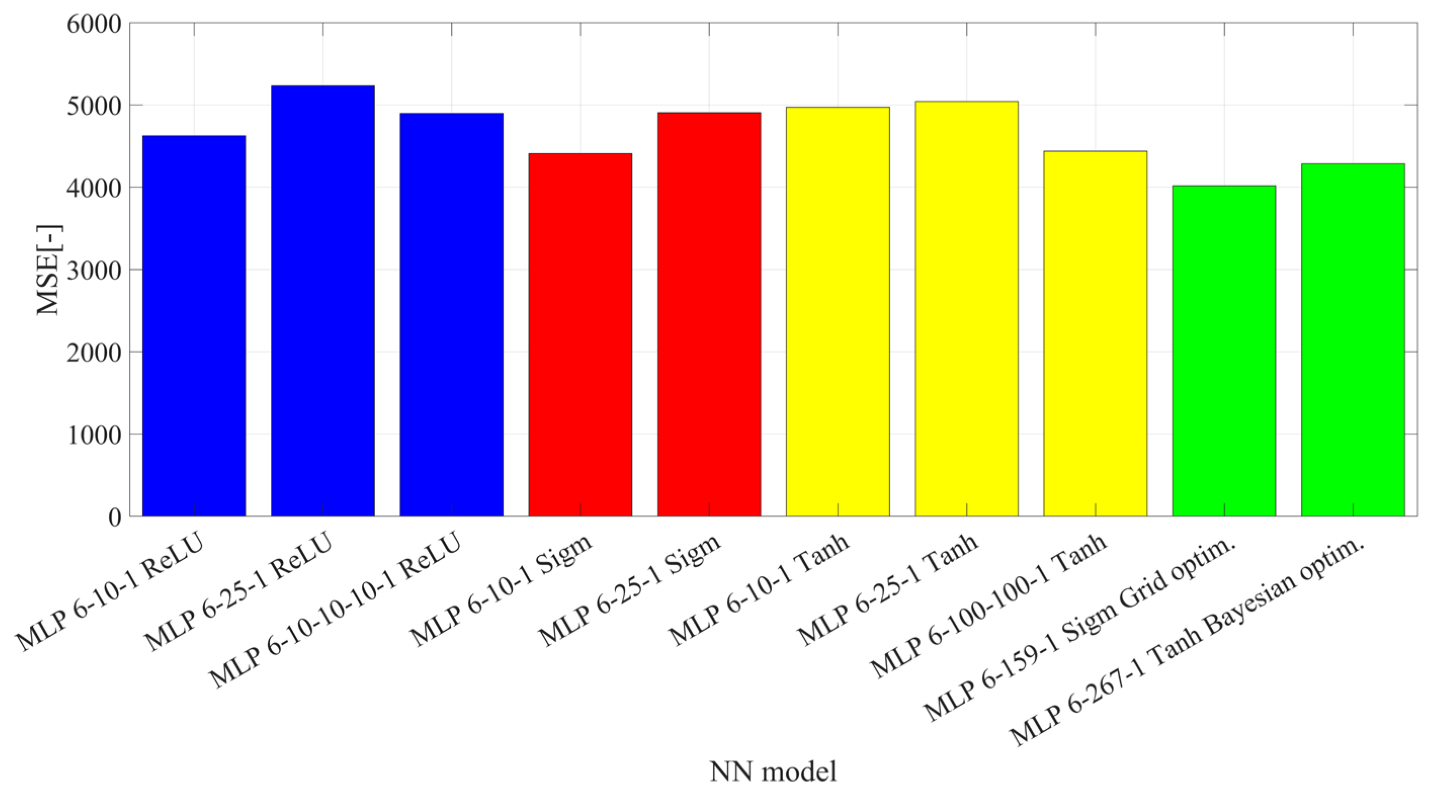
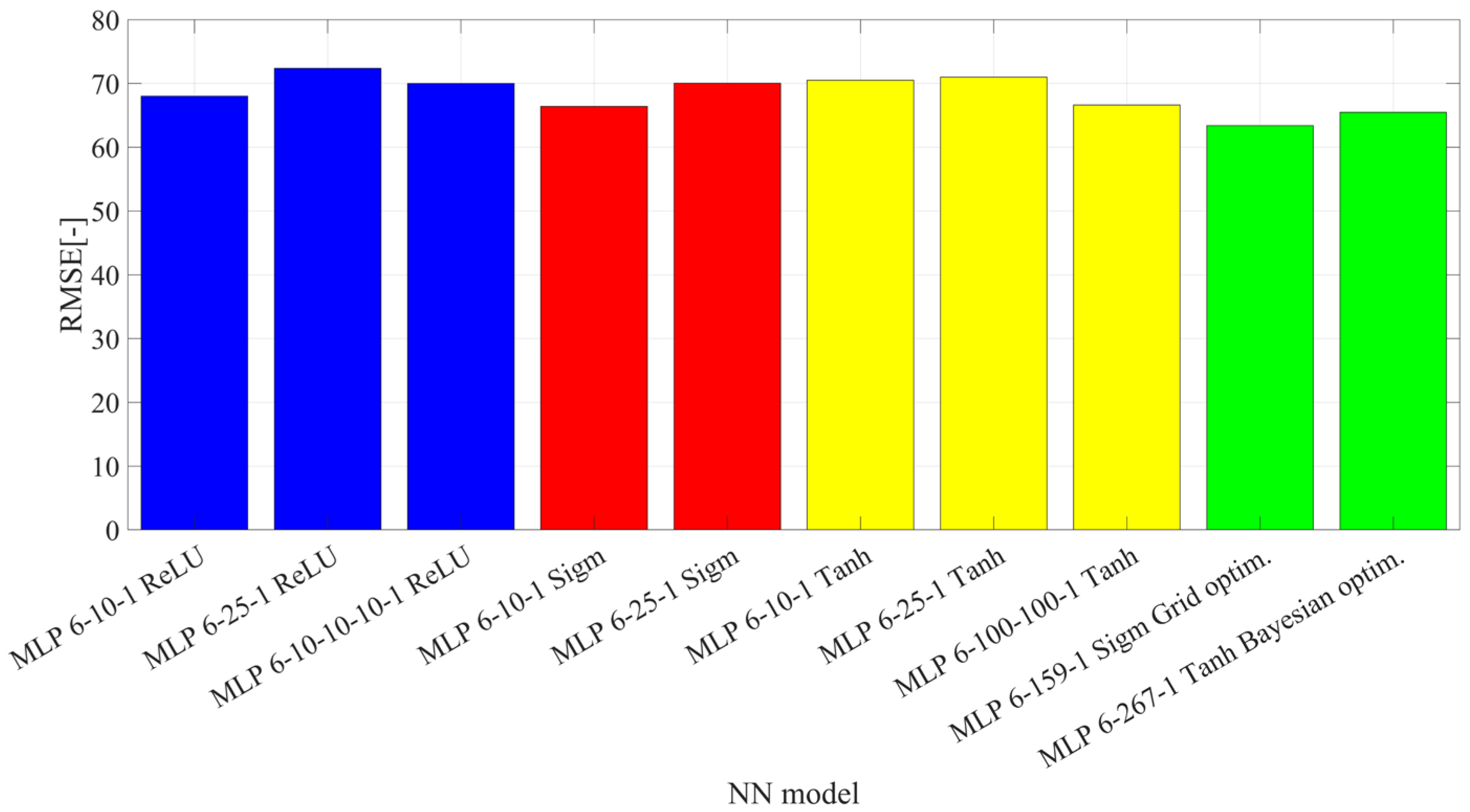
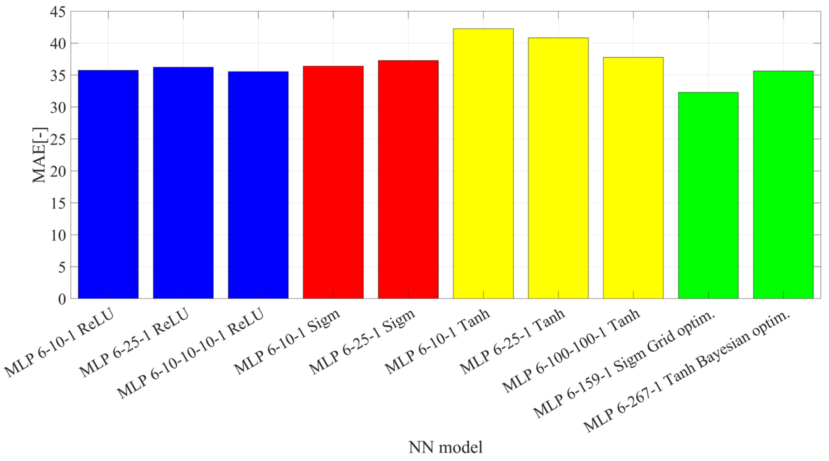
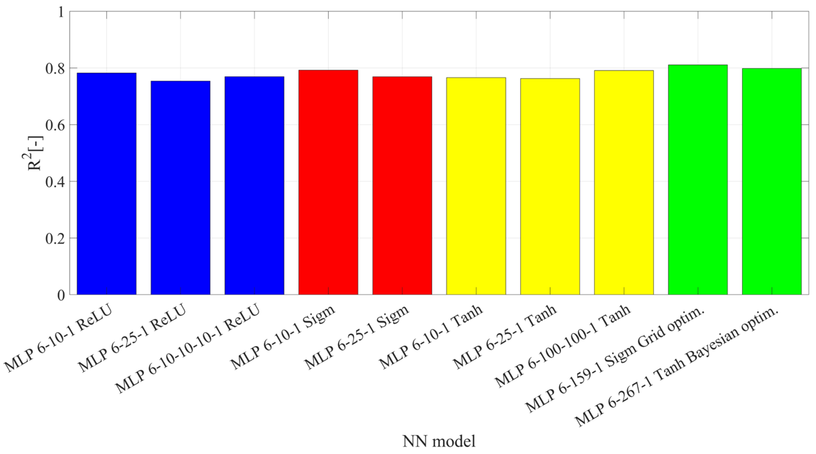
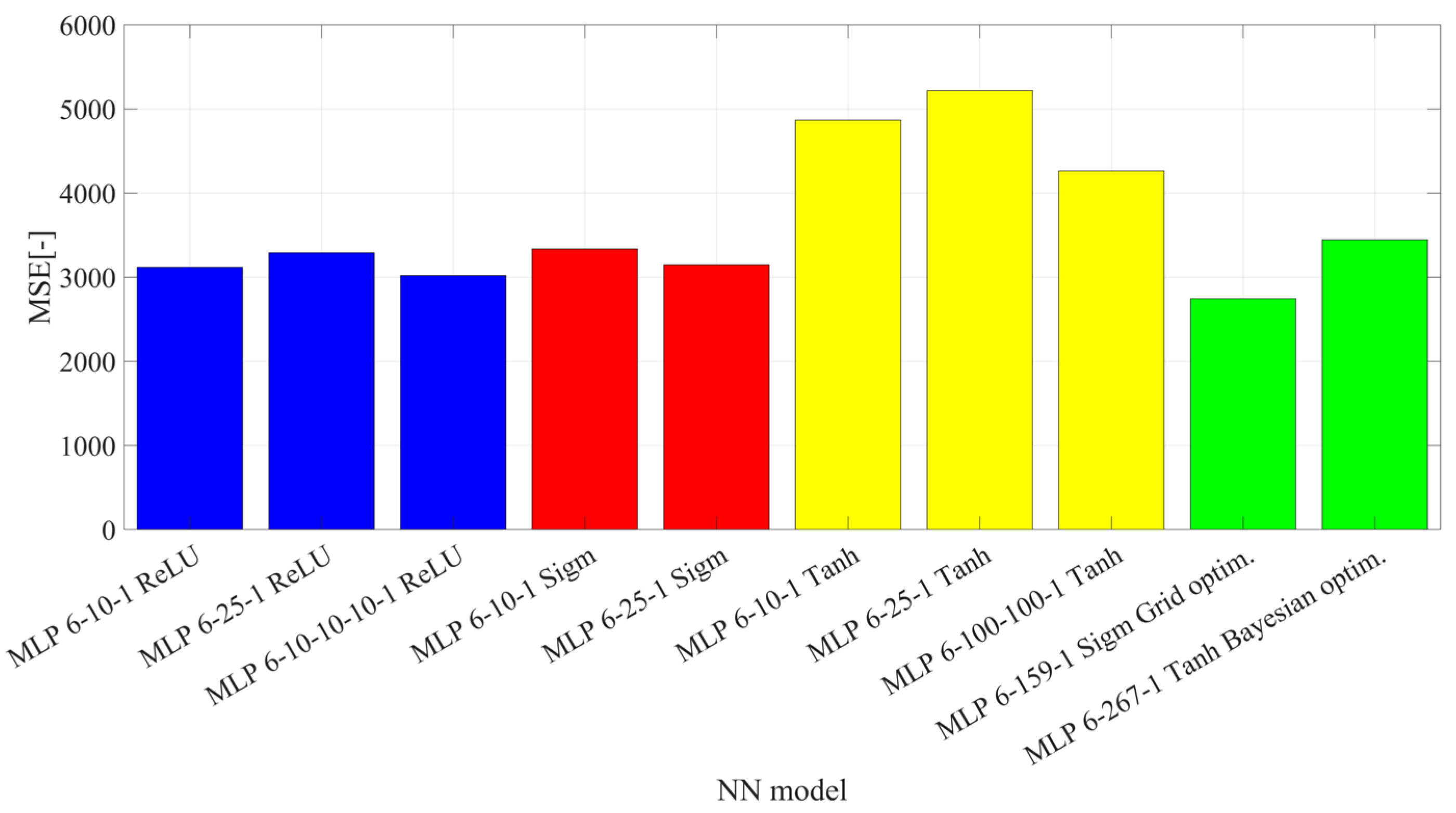
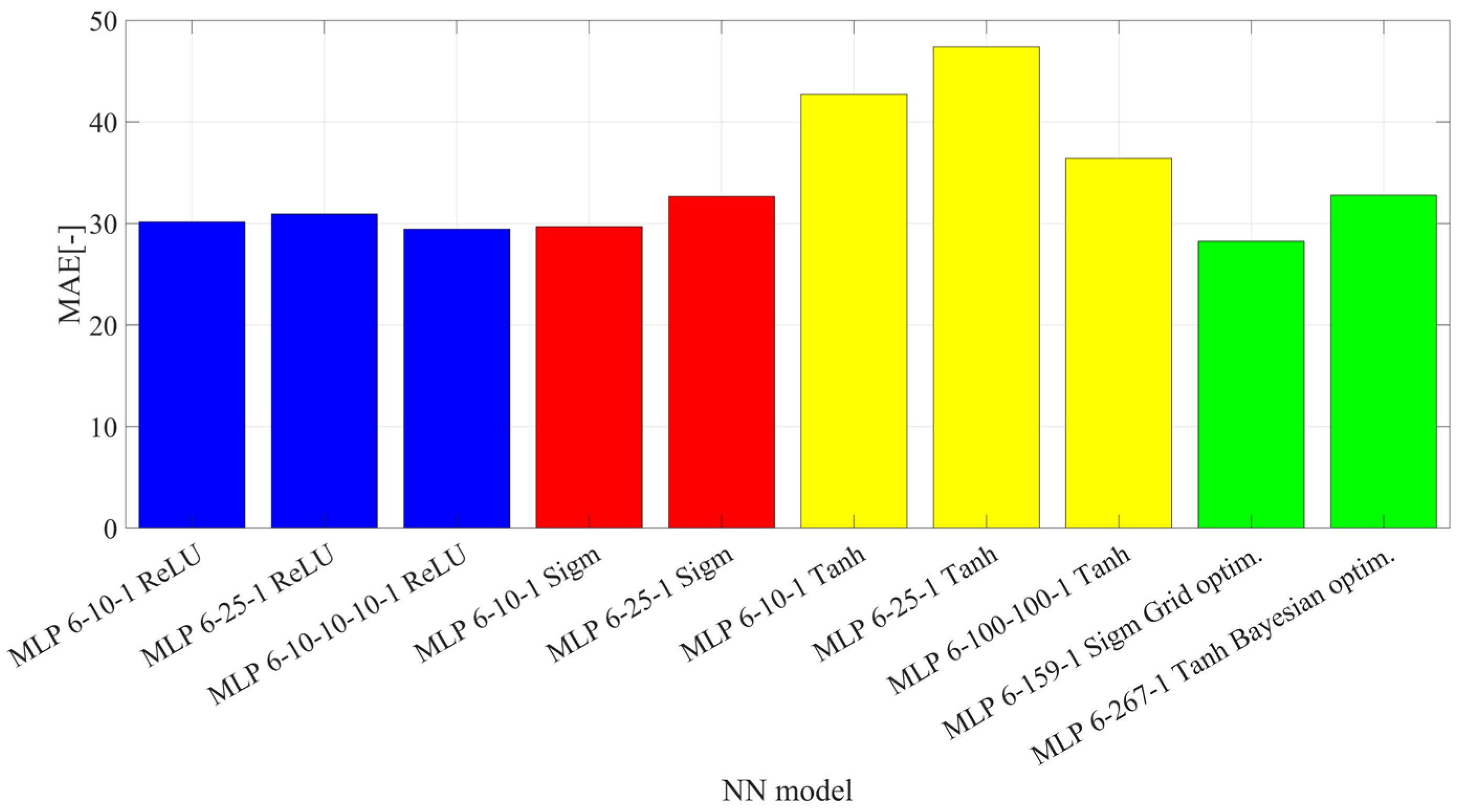
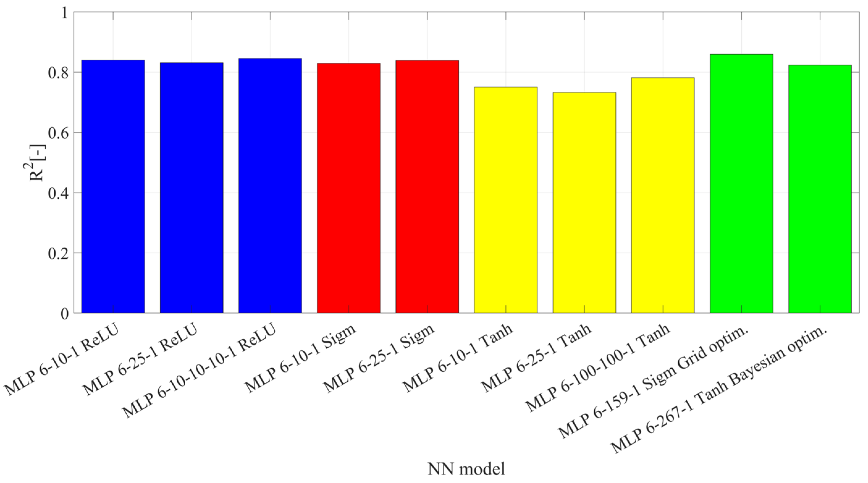
Figure 11, Figure 12, Figure 13, Figure 14, Figure 15, Figure 16, Figure 17 and Figure 18 present the results of quality indicators of ten neural networks with the highest values of the obtained coefficient of determination R2, both during validation and testing.
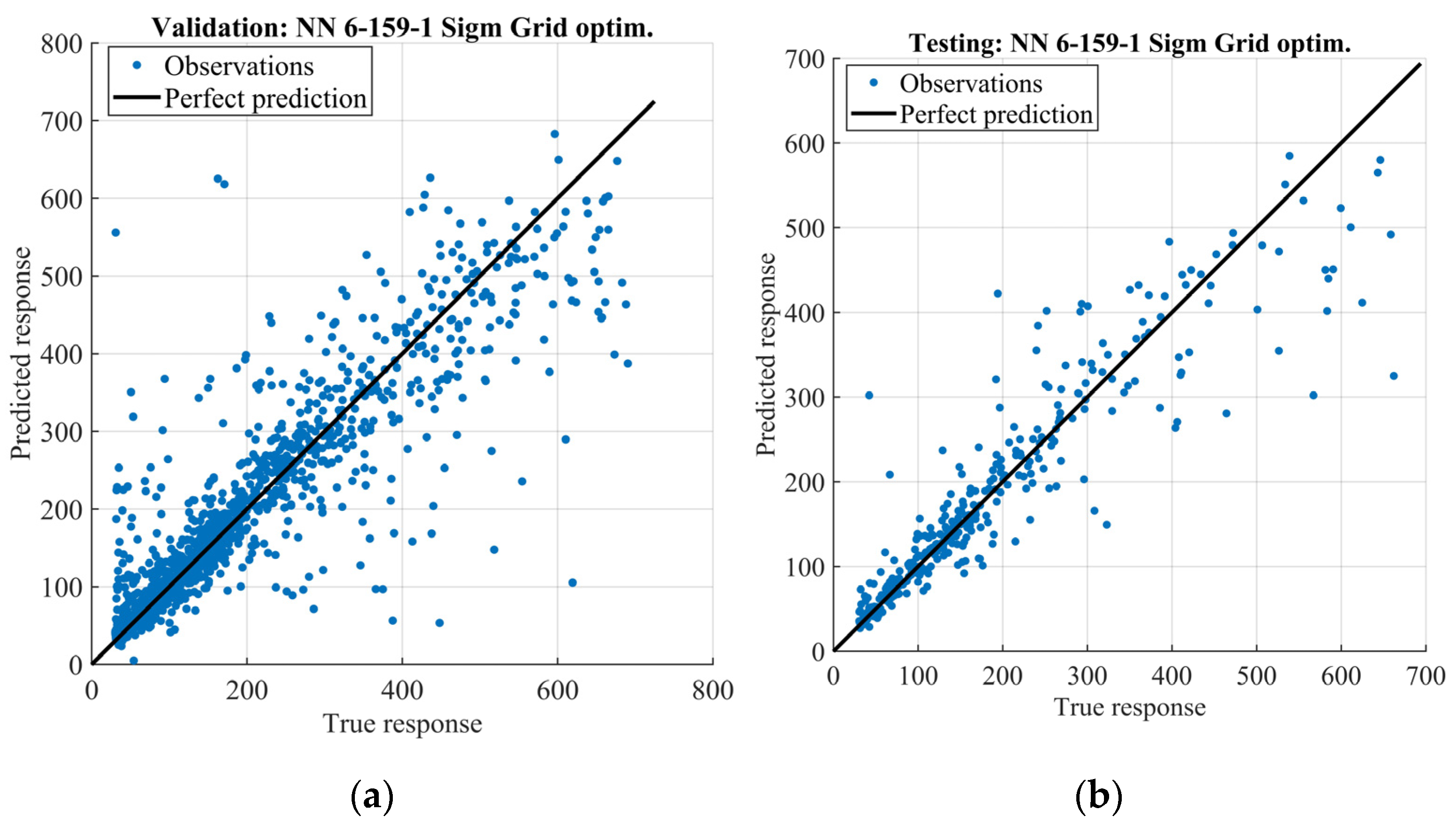
The quality indicator values presented in Figure 18 show significant differences in the performance of individual models. The network model that yielded the lowest MAE, MSE, and RMSE values and showed the highest R2 during validation was the MLP 6-159-1 model with a sigmoid activation function, optimised using the Grid Search method. In turn, the network model among those not subject to optimisation that achieved the best results in the above-mentioned indicators during validation was the MLP 6-10-1 model with a sigmoid function. In the test data, the model that yielded the lowest MAE, MSE, and RMSE values and the highest R2 was also the MLP 6-159-1 model with a sigmoid function.
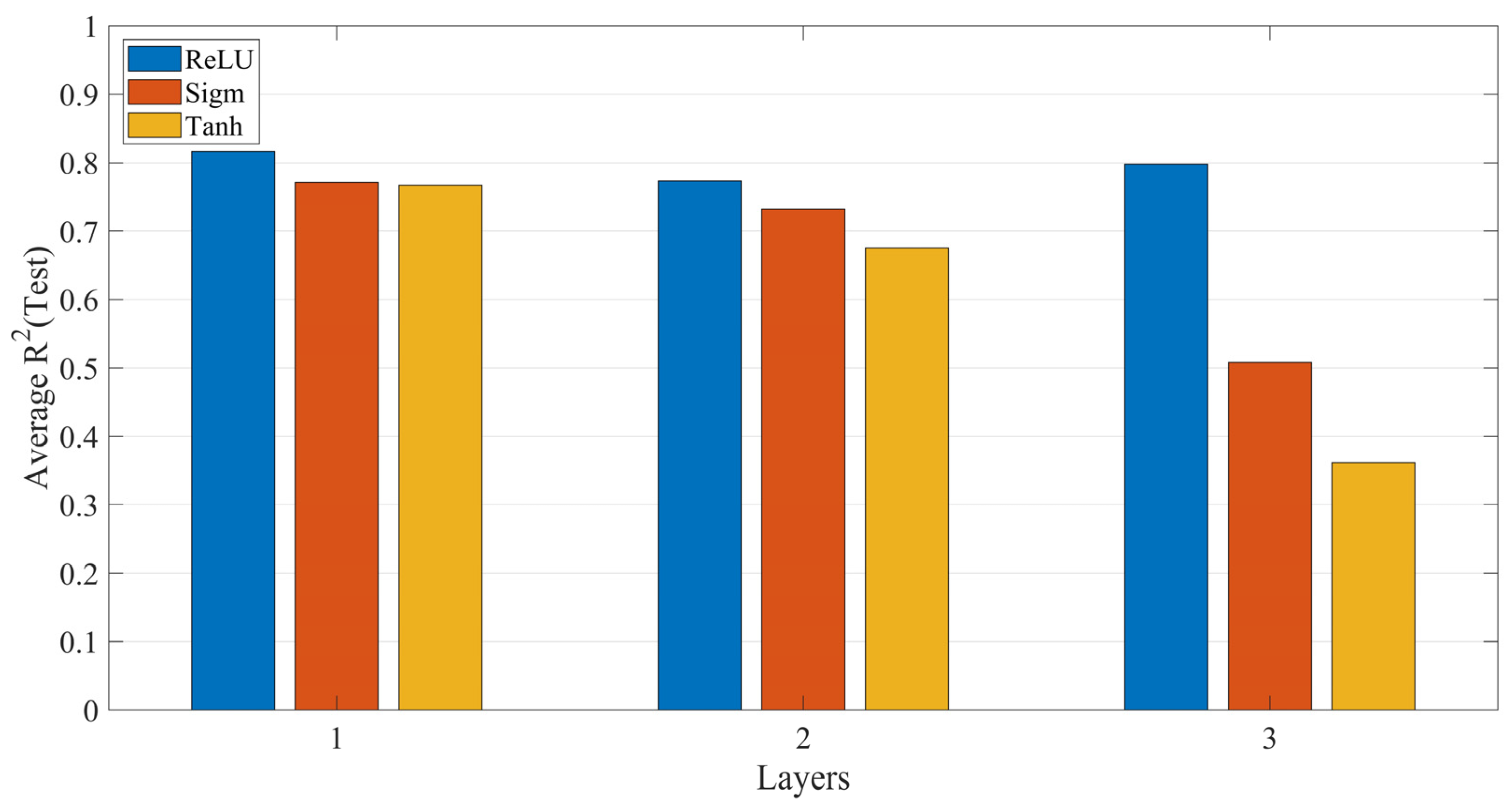
The average R2 values for the test data, as a function of the number of hidden layers and the activation function, are shown in Figure 19.
The results show that, in the analysed case, neural networks with one hidden layer achieve the highest average coefficient of determination (R2). The activation function that achieves the highest value of the mentioned indicator, regardless of the number of layers, is ReLU. Figure 19 also shows a clear degradation in results for the sigmoid and hyperbolic tangent activation functions in models with more than one layer (two or three). The high results for the ReLU function are due to its simple mathematical relation (relation (3)), which is particularly useful to reduce the computational complexity for networks with more than one hidden layer.
In turn, Figure 20 presents the neural network’s prediction results, which yielded the best R2 coefficient during both testing and validation, i.e., the NN 6-159-1 Sigm network with the Grid search algorithm optimisation applied.
The constructed models achieve high values of the coefficient of determination (R2) in the testing phase, of the order of 0.8 (Figure 18), and, in some cases, exceed those obtained in the validation phase (Figure 14), confirming the neural network models’ high generalisation and accuracy.

4. Discussion

Altitude above sea level and engine speed were excluded from the neural network model development process due to low F-test, MRMR, and ReliefF values, and low correlation with the output variable (CO2 emissions).
The best NN model in the study achieved R2 ≈ 0.86 using sigmoid functions with six features. In the article [17], very high R2 values were achieved (0.9979 for XGB, 0.9966 for Random Forest, 0.9957 for CNN). The authors used 7384 vehicle records from the Canadian Government database with 19 features. In turn, in the article, authors [9] achieved R2 ≈ 0.85 using MLP with Bayesian optimization on real-world Real Driving Emissions test data with approximately 570,000 samples. Authors of the article [11] used LSTM for OBD-II data but did not report R2 values, making direct comparison difficult.
The article considers three selected characteristic activation functions. The first is the sigmoid function, which, due to its mathematical dependence and the exponential function within it, is characterized by a nonlinear behavior and takes values in the range (0, 1). The second function under consideration is the hyperbolic tangent function, a modification of the sigmoid function. It is characterized by a range of values in (−1, 1) that is symmetric about zero. The presence of exponential dependencies in both functions increases their computational complexity and influences their application. The last analysed activation function is ReLU, which is characterized by a linear dependence ensuring computational simplicity. ReLU is the default activation function in hidden layers used in modern MLP models and more complex network models, such as CNNs.
Another parameter of neural networks analysed in this article is the number of hidden layers, which determines the network’s depth and influences its learning ability, particularly for nonlinear dependencies present in the analysed data. The obtained results indicate that the activation function has little impact on model results for the simplest variant of neural networks, i.e., with a single hidden layer.
In this case, the number of neurons in the hidden layer is the most crucial factor influencing network performance (as reflected in the quality indicator values). In the case of two and three hidden layers, due to the significantly different quality indicator results, activation functions have a greater impact on network performance. Each additional hidden layer increases the network’s approximation ability and allows it to represent increasingly complex nonlinear patterns, but it also increases the risk of overfitting. Increased network depth also means more network weights are updated during training, which is one of the reasons for the reduced R2 values in networks with more than one hidden layer. The research results also clearly indicate that networks with three hidden layers require selecting the number of neurons per layer and the type of activation function to achieve the desired performance. Given the limited data presented in this article, originating from a single vehicle, a deeper network architecture (especially with three hidden layers) leads to a deterioration in network performance. The research also shows that network performance is not directly proportional to the number of layers; the network development process requires experimental adaptation to the specific problem.
For the analysed dataset, neural networks with a single hidden layer yielded the best results on the quality indicators. There was no direct correlation between the number of neurons and the number of hidden layers on the quality indicator values of neural networks.
The ReLU function provides the highest coefficient of determination values for 1, 2, and 3 hidden layers. The sigmoid and hyperbolic tangent functions perform best for MLP networks with a single hidden layer; however, with more layers, the quality metrics, including the coefficient of determination, decrease significantly.
The analysed neural network optimisation methods, i.e., Grid search and Bayesian optimisation, although very time-consuming and computationally demanding, confirmed their usefulness by generating network models with the best quality indicators.

5. Conclusions

MLP neural networks of various architectures with 1, 2, or 3 hidden layers can be used to model CO2 emissions from motor vehicles.
Selecting the appropriate network structure requires experimental research. The number of hidden layers must be carefully selected. However, the study shows that the best practice is to start with single-layer neural networks with the ReLU activation function and a small number of neurons, gradually increasing the number of neurons and hidden layers.
There are significant interactions between neural network parameters: the choice of activation function depends on network depth.
Activation functions have a significant impact on neural network performance. The ReLU function is the most universal activation function, providing high indicator values that are consistent across the number of hidden layers. However, it was the non-linear activation functions subjected to the optimization process that allowed the best neural network to be obtained in terms of the R2 coefficient during both testing and validation.
The final choice of neural network architecture depends on the quality of the data set and the expectations regarding accuracy; however, the optimisation processes for constructing neural networks, i.e., Grid search or Bayesian optimisation, can facilitate finding the desired network structure.
Limiting the study to a single vehicle reduces the representativeness of the results. The conclusions drawn from a single car cannot be generalized to a larger number of vehicles.
Further research could lead to the implementation of comprehensive driving assistance systems in vehicles, helping drivers adapt their driving style. The developed model for real-time monitoring and analysis of measured parameters opens new perspectives for the development of intelligent CO2 emission management systems in vehicles, as well as for more effective emission-reduction strategies in road transport. Further research could also explore architectural optimization, e.g., by using different activation functions across layers, which could lead to better results than a single activation function for the entire network, as assumed in the work.

Funding

This research was funded by the Military University of Technology under the research project UGB 22/WLO/2025.

Institutional Review Board Statement

Not applicable.

Informed Consent Statement

Not applicable.

Data Availability Statement

The data presented in this study are available on request from the author of the article.

Conflicts of Interest

The author declares no conflicts of interest.

Abbreviations

The following abbreviations are used in this manuscript:
BFGSBroyden–Fletcher–Goldfarb–Shanno
CNNConvolutional Neural Network
GNSSGlobal Navigation Satellite System
HDOPHorizontal Dilution of Precision
IMUInertial Measurement Unit
LTSMLong Short-Term Memory
MAEMean Absolute Error
MLPMulti-Layer Perceptron
MRMRMinimum Redundancy Maximum Relevance
MSEMean Squared Error
OBDOn-Board Diagnostics
PEMSPortable Emissions Measurement System
ReLURectified Linear Unit
RMSERoot Mean Squared Error
RReliefFRegressional ReliefF
XAIExplainable Artificial Intelligence

Appendix A

Velocity accuracy in GNSS systems is an essential issue for many applications, including transportation. Research indicates a strong correlation between satellite constellation geometry and velocity measurement accuracy, as assessed by the HDOP parameter (Figure A1) and the number of available satellites (Figure A2).
Figure A1. Time variation in the HDOP parameter.
Applsci 15 12037 g0a1
Figure A2. Time variation in the number of satellites.
Applsci 15 12037 g0a2
HDOP is the dominant parameter describing the effect of geometry on measurement precision. Furthermore, there is a strong negative relationship between the number of satellites and the HDOP coefficient. Empirical studies of velocity determination in GNSS systems using Doppler measurements demonstrate a close relationship between the number of available satellites and the RMS error in velocity. To determine velocity, the theoretical minimum number of satellites is 4. In practice, it is recommended to have access to at least 6–8 satellites to achieve acceptable accuracy. The accuracy mentioned above is also achieved when the HDOP parameter meets the condition HDOP < 5. Determining the value of velocity errors requires experimental testing of the GNSS receiver used in the research [37,38,39].

Appendix B

Although OBD-II is a mandatory standard, its implementation by vehicle manufacturers varies. The same parameter can be calculated differently across brands and models, making it difficult to generalize about accuracy levels. Therefore, the accuracy of measurements using the OBD interface varies significantly. Determining measurement errors requires experimental studies. PEMS systems are used to determine accurate CO2 emission measurements [40].

References

  1. Kopfer, H.W.; Schönberger, J.; Kopfer, H. Reducing greenhouse gas emissions of a heterogeneous vehicle fleet. Flex. Serv. Manuf. J. 2014, 26, 221–248. [Google Scholar] [CrossRef]
  2. Folęga, P.; Burchart, D.; Kubik, A.; Turoń, K. Application of the life cycle assessment method in public bus transport. Eksploat. Niezawodn. Maint. Reliab. 2025, 27, 204539. [Google Scholar] [CrossRef]
  3. Adamiak, B.; Andrych-Zalewska, M.; Merkisz, J.; Chłopek, Z. The uniqueness of pollutant emission and fuel consumption test results for road vehicles tested on a chassis dynamometer. Eksploat. Niezawodn. Maint. Reliab. 2025, 27, 195747. [Google Scholar] [CrossRef]
  4. Biszko, K.; Oskarbski, J. Modelowanie emisji z wykorzystaniem symulacji mikroskopowych. Transp. Miej. Reg. 2022, 5, 18–25. [Google Scholar]
  5. Rykała, M.; Grzelak, M.; Rykała, Ł.; Voicu, D.; Stoica, R.-M. Modeling Vehicle Fuel Consumption Using a Low-Cost OBD-II Interface. Energies 2023, 16, 7266. [Google Scholar] [CrossRef]
  6. Matijošius, J.; Žvirblis, T.; Rimkus, A.; Stravinskas, S.; Kilkevičius, A. Emissions, reliability and maintenance aspects of a dual-fuel engine (diesel-natural gas) using HVO additive and ANCOVA modeling. Eksploat. Niezawodn. Maint. Reliab. 2026, 28. [Google Scholar] [CrossRef]
  7. Mungan, M.S.; Arpa, O. Estimation of CO2 emissions from vehicles using machine learning and multi-model investigation. Bull. Pol. Acad. Sci. Tech. Sci. 2025, 73, e154287. [Google Scholar] [CrossRef]
  8. Brzezinski, M.; Kijek, M.; Gontarczyk, M.; Rykala, L.; Zelkowski, J. Fuzzy Modeling of Evaluation Logistic Systems. In Proceedings of the 21st International Conference, Transport Means, Juodkrante, Lithuania, 20–22 September 2017; pp. 377–382. [Google Scholar]
  9. Donateo, T.; Filomena, R. Real time estimation of emissions in a diesel vehicle with neural networks. In Proceedings of the E3S Web of Conferences, EDP Sciences, 75th National ATI Congress, Rome, Italy, 15–16 September 2020; Volume 197, p. 06020. [Google Scholar]
  10. Li, X.; Song, K.; Shi, J. Degradation generation and prediction based on machine learning methods: A comparative study. Eksploat. Niezawodn. Maint. Reliab. 2025, 27, 192168. [Google Scholar] [CrossRef]
  11. Singh, M.; Dubey, R.K. Deep learning model based CO2 emissions prediction using vehicle telematics sensors data. IEEE Trans. Intell. Veh. 2021, 8, 768–777. [Google Scholar] [CrossRef]
  12. Alam, G.M.I.; Arfin Tanim, S.; Sarker, S.K.; Watanobe, Y.; Islam, R.; Mridha, M.F.; Nur, K. Deep learning model based prediction of vehicle CO2 emissions with eXplainable AI integration for sustainable environment. Sci. Rep. 2025, 15, 3655. [Google Scholar] [CrossRef] [PubMed]
  13. Selvam, H.P.; Li, Y.; Wang, P.; Northrop, W.F.; Shekhar, S. Vehicle emissions prediction with physics-aware ai models: Preliminary results. arXiv 2021, arXiv:2105.00375. [Google Scholar] [CrossRef]
  14. Michailidis, E.T.; Panagiotopoulou, A.; Papadakis, A. A Review of OBD-II-Based Machine Learning Applications for Sustainable, Efficient, Secure, and Safe Vehicle Driving. Sensors 2025, 25, 4057. [Google Scholar] [CrossRef]
  15. Mostafa, N.N.; Tolba, A.; Abouhawwash, M. Application of Deep Learning Initiatives for CO2 Emissions Forecasting. Clim. Change Rep. 2024, 1, 19–29. [Google Scholar] [CrossRef]
  16. Li, S.; Tong, Z.; Haroon, M. Estimation of transport CO2 emissions using machine learning algorithm. Transp. Res. Part D Transp. Environ. 2024, 133, 104276. [Google Scholar] [CrossRef]
  17. Gurcan, F. Forecasting CO2 emissions of fuel vehicles for an ecological world using ensemble learning, machine learning, and deep learning models. PeerJ Comput. Sci. 2024, 10, e2234. [Google Scholar] [CrossRef]
  18. Pinto, G.; Oliver-Hoyo, M.T. Using the relationship between vehicle fuel consumption and CO2 emissions to illustrate chemical principles. J. Chem. Educ. 2008, 85, 218. [Google Scholar] [CrossRef]
  19. Fontaras, G.; Zacharof, N.G.; Ciuffo, B. Fuel consumption and CO2 emissions from passenger cars in Europe–Laboratory versus real-world emissions. Prog. Energy Combust. Sci. 2017, 60, 97–131. [Google Scholar] [CrossRef]
  20. Adamiak, B.; Szczotka, A.; Woodburn, J.; Merkisz, J. Comparison of exhaust emission results obtained from Portable Emissions Measurement System (PEMS) and a laboratory system. Combust. Engines 2023, 62, 128–135. [Google Scholar] [CrossRef]
  21. Merkisz, J.; Rymaniak, Ł. Determining the environmental indicators for vehicles of different categories in relation to CO2 emission based on road tests. Combust. Engines 2017, 56, 66–72. [Google Scholar] [CrossRef]
  22. Merkisz, J.; Dobrzynski, M.; Kubiak, K. An impact assessment of functional systems in vehicles on CO2 emissions and fuel consumption. MATEC Web Conf. 2017, 118, 00030. [Google Scholar] [CrossRef]
  23. Lasocki, J.; Chłopek, Z.; Godlewski, T. Driving style analysis based on information from the vehicle’s OBD system. Combust. Engines 2019, 58, 173–181. [Google Scholar] [CrossRef]
  24. Puchalski, A.; Komorska, I. Driving style analysis and driver classification using OBD data of a hybrid electric vehicle. Transp. Probl. 2020, 15, 83–94. [Google Scholar] [CrossRef]
  25. Ericsson, E. Independent driving pattern factors and their influence on fuel-use and exhaust emission factors. Transp. Res. Part D Transp. Environ. 2001, 6, 325–345. [Google Scholar] [CrossRef]
  26. Rykała, Ł.; Rubiec, A.; Przybysz, M.; Krogul, P.; Cieślik, K.; Muszyński, T.; Rykała, M. Research on the Positioning Performance of GNSS with a Low-Cost Choke Ring Antenna. Appl. Sci. 2023, 13, 1007. [Google Scholar] [CrossRef]
  27. Malon, K.; Łopatka, J.; Rykała, Ł.; Łopatka, M. Accuracy Analysis of UWB Based Tracking System for Unmanned Ground Vehicles. In Proceedings of the 2018 New Trends in Signal Processing (NTSP), Demänovská Dolina, Slovakia, 10–12 October 2018; pp. 1–7. [Google Scholar]
  28. Cellina, M.; Strada, S.; Savaresi, S.M. Vehicle fuel consumption virtual sensing from GNSS and IMU measurements. In Proceedings of the 2023 IEEE 26th International Conference on Intelligent Transportation Systems (ITSC), Bilbao, Spain, 24–28 September 2023; IEEE: Piscataway, NJ, USA, 2023; pp. 488–493. [Google Scholar]
  29. Andrych-Zalewska, M.; Chłopek, Z.; Merkisz, J.; Pielecha, J. Research on the results of the WLTP procedure for a passenger vehicle. Maint. Reliab. Eksploat. Niezawodn. 2024, 26, 176112. [Google Scholar] [CrossRef]
  30. Feature Selection. Available online: https://www.mathworks.com/help/stats/feature-selection.html (accessed on 15 September 2025).
  31. Yuan, L.; Lu, W.; Xue, F.; Li, M. Building feature-based machine learning regression to quantify urban material stocks: A Hong Kong study. J. Ind. Ecol. 2023, 27, 336–349. [Google Scholar] [CrossRef]
  32. Neural Networks: Activation functions. Available online: https://developers.google.com/machine-learning/crash-course/neural-networks/activation-functions?hl=pl (accessed on 15 September 2025).
  33. Osowski, S.; Cichocki, A.; Siwek, K. MATLAB w Zastosowaniu do Obliczeń Obwodowych i Przetwarzania Sygnałów; Oficyna Wydawnicza Politechniki Warszawskiej: Warsaw, Poland, 2006. [Google Scholar]
  34. Rykała, M.; Rykała, Ł. Economic Analysis of a Transport Company in the Aspect of Car Vehicle Operation. Sustainability 2021, 13, 427. [Google Scholar] [CrossRef]
  35. Osowski, S. Metody i narzędzia eksploracji danych; BTC: Warsaw, Poland, 2013. [Google Scholar]
  36. Rykała, M. A Study of the CO2 Emissions of a Passenger Vehicle on a Selected Example Using Mathematical Methods. Ph.D. Thesis, Military University of Technology, Warsaw, Poland, 2025. [Google Scholar]
  37. Li, Y.; Wang, L.; Liu, J.; Zhang, P.; Lu, Y. Accuracy evaluation of multi-GNSS Doppler velocity estimation using android smartphones. Int. Arch. Photogramm. Remote Sens. Spat. Inf. Sci. 2022, 46, 89–96. [Google Scholar] [CrossRef]
  38. Specht, M. Experimental studies on the relationship between HDOP and position error in the GPS system. Metrol. Meas. Syst. 2022, 29, 17–36. [Google Scholar] [CrossRef]
  39. Gao, G.X.; Enge, P. How many GNSS satellites are too many? IEEE Trans. Aerosp. Electron. Syst. 2012, 48, 2865–2874. [Google Scholar] [CrossRef]
  40. Ragab, H.; Givigi, S.; Noureldin, A. Automotive speed estimation: Sensor types and error characteristics from obd-ii to adas. In Proceedings of the 2025 IEEE/ION Position, Location and Navigation Symposium (PLANS), Salt Lake City, UT, USA, 28 April–1 May 2025; IEEE: Piscataway, NJ, USA, 2025; pp. 124–130. [Google Scholar]
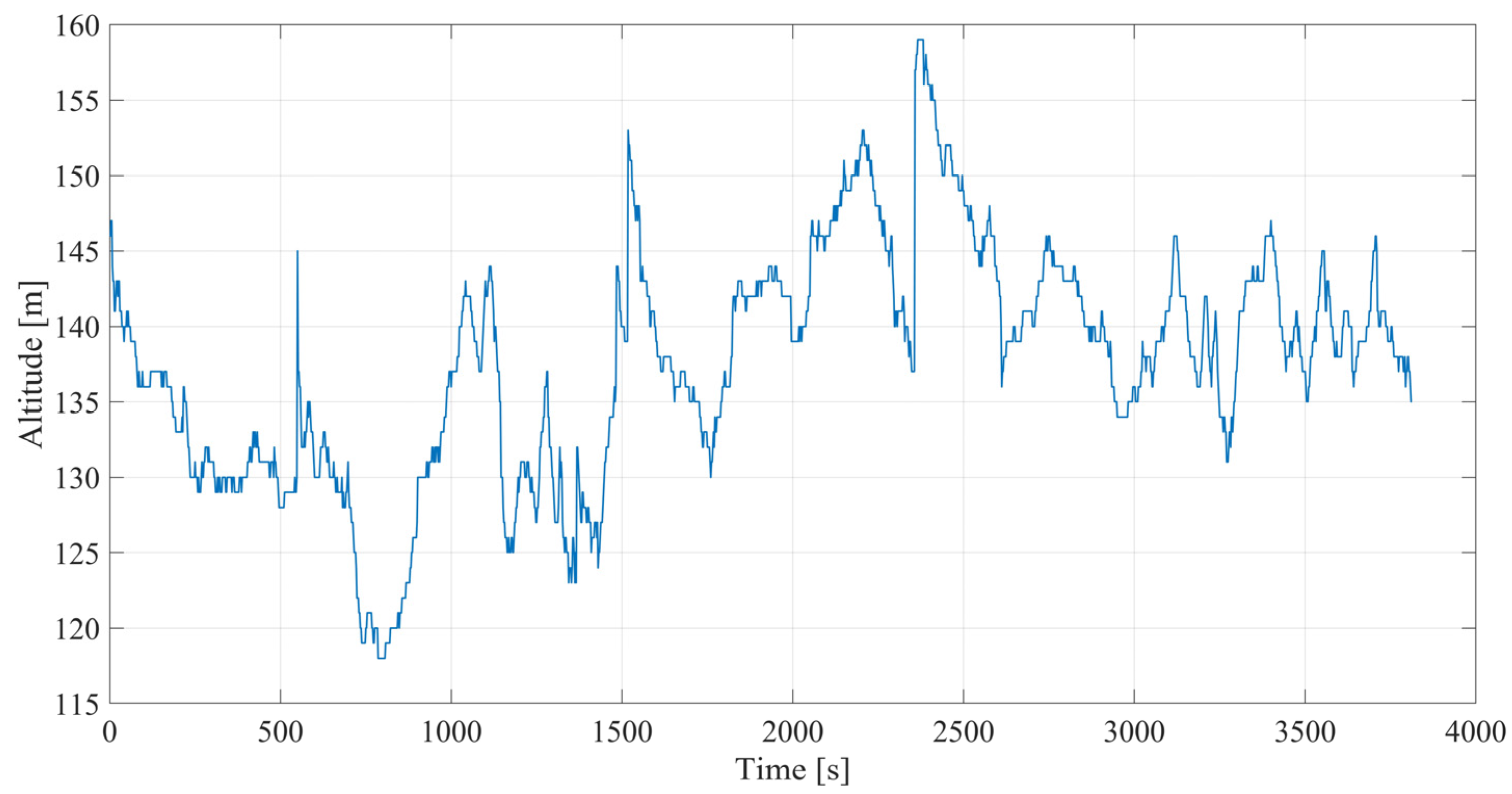
Figure 1. Time variation in the altitude.
Applsci 15 12037 g001
Figure 2. Time variation in the vehicle acceleration.
Applsci 15 12037 g002
Figure 3. Time variation in the vehicle speed.
Applsci 15 12037 g003
Figure 4. Time variation in the engine load.
Applsci 15 12037 g004
Figure 5. Time variation in the engine speed.
Applsci 15 12037 g005
Figure 6. Time variation in the throttle position.
Applsci 15 12037 g006
Figure 7. Time variation in the CO2 emissions.
Applsci 15 12037 g007
Figure 8. Results of the F-test algorithm performed on the data set.
Applsci 15 12037 g008
Figure 9. Results of the MRMR algorithm performed on the data set.
Applsci 15 12037 g009
Figure 10. Results of the RReliefF algorithm performed on the data set.
Applsci 15 12037 g010
Figure 11. Results of the MSE indicator during validation for selected neural networks.
Applsci 15 12037 g011
Figure 12. Results of the RMSE indicator during validation for selected neural networks.
Applsci 15 12037 g012
Figure 13. Results of the MAE indicator during validation for selected neural networks.
Applsci 15 12037 g013
Figure 14. Results of the R2 indicator during validation for selected neural networks.
Applsci 15 12037 g014
Figure 15. Results of the MSE indicator during testing for selected neural networks.
Applsci 15 12037 g015
Figure 16. Results of the RMSE indicator during testing for selected neural networks.
Applsci 15 12037 g016
Figure 17. Results of the MAE indicator during testing for selected neural networks.
Applsci 15 12037 g017
Figure 18. Results of the R2 indicator during testing for selected neural networks.
Applsci 15 12037 g018
Figure 19. The average value of the coefficient of determination R2 for the test data, depending on the number of hidden layers and the used activation function.
Applsci 15 12037 g019
Figure 20. Prediction results from NN 6-159-1 Sigm with Grid optimisation during (a) validation, (b) testing.
Applsci 15 12037 g020
Table 1. Selected Technical specifications of the vehicle [5].
ParameterData
ManufacturerMazda
Model3
Body typeSedan
Weight1280 kg
FuelGasoline
Engine displacement1998 cm3
Maximum engine power 88 kW at 6000 rpm
CO2 emission norm EURO 5
Table 2. Data specifications.
Parameter TypeParameter NameDetails
InputAltitude (m)Read from GNSS
InputVehicle speed (km/h)Read from GNSS
InputVehicle acceleration (m/s2)Calculated from vehicle speed
InputEngine load (%)Read from OBD
InputEngine speed (rpm)Read from OBD
InputThrottle position (%)Read from OBD
OutputCO2 emission (g/km)Read from OBD
Table 3. Descriptive statistics of variables.
VariableMinimumMeanStd. Dev.Maximum
Altitude (m)118.00137.597.59159.00
Vehicle speed (km/h)1.2642.2326.17105.44
Vehicle acceleration (m/s2)−6.09−0.041.265.32
Engine load (%)8.6229.2419.67100.00
Engine speed (rpm)509.751572.88499.752699.75
Throttle position (%)0.038.649.9682.35
Table 4. Correlation between the dependent variable and the independent quantitative variables.
VariableCO2 Emission
Altitude (m)0.05
Vehicle speed (km/h)−0.30
Vehicle acceleration (m/s2)0.39
Engine load (%)0.69
Engine speed (rpm)−0.19
Throttle position (%)0.44
Disclaimer/Publisher’s Note: The statements, opinions and data contained in all publications are solely those of the individual author(s) and contributor(s) and not of MDPI and/or the editor(s). MDPI and/or the editor(s) disclaim responsibility for any injury to people or property resulting from any ideas, methods, instructions or products referred to in the content.