B-Value Spatiotemporal Changes and Aftershock Correlation Prior to the M_wg 7.1 Dingri Earthquake in Southern Tibet: Implications for Land Deformation and Seismic Risk

Abstract

This study investigates spatiotemporal b value variations and seismic interaction networks preceding the M_wg 7.1 Dingri earthquake that struck southern Tibet on 7 January 2025. Using relocated earthquake catalogs (2021–2025) and dual-method analysis combining b value mapping with Granger causality network modeling, we reveal systematic precursory patterns. Spatial analysis shows that the most significant b value reduction (Δb > 0.5) occurred north of the mainshock epicenter at seismogenic depths (5–15 km), closely aligning with subsequent aftershock concentration zones. Granger causality analysis reveals a progressive network simplification: from 73 causal links among 28 nodes during the background period (2021–2023) to 49 links among 34 nodes pre-mainshock (2023–2025) and finally to 6 localized links post-rupture. This transition from distributed system-wide interactions to localized “locked-in” dynamics reflects the stress concentration onto the primary asperity approaching critical failure. The convergence of b value anomalies and network evolution provides a comprehensive framework linking quasi-static stress states with dynamic system behavior. These findings offer valuable insights for understanding earthquake nucleation processes and improving seismic hazard assessment in the Tibetan Plateau and similar complex tectonic environments.

1. Introduction

The magnitude-frequency distribution of earthquakes, first described by Ishimoto and Iida [1] and later formalized as the Gutenberg–Richter relation [2], can be represented in seismically active regions as

$${\mathrm{l}\mathrm{o}\mathrm{g}}_{10}N=a-bM$$

(1)

where M is the earthquake magnitude, N is the cumulative number of earthquakes with magnitude greater than or equal to M, and a and b are constants. The b value represents the ratio between the numbers of small and large earthquakes. Globally, statistical analysis shows that the b value is close to 1.0 over large regional scales [3]. However, within smaller spatial scales (from several to tens of kilometers), the b value can vary significantly in both space and time. For example, in Japan, the b value ranges from 0.5 to 1.5 [4], while in the Parkfield region along the San Andreas Fault, it varies between 0.5 and 1.3 [5]. Variations in the b value of a region are typically associated with its seismic activity characteristics. For instance, regions near magma chambers may exhibit high b values [6,7]. In contrast, the initial rupture zones of large earthquakes often occur in areas with low b values [8,9]. Previous studies have indicated that low b value regions imply higher differential stress and suggest that these areas may be near the end of the seismic cycle. This relationship has been used for seismic hazard assessment and earthquake forecasting, although the effectiveness of earthquake forecasting experiments remains controversial [10,11,12,13].

Due to the collision between the Indian and Eurasian plates, a large number of earthquakes have occurred in the Tibetan Plateau and its surrounding regions. The M_wg 7.1 earthquake that struck Dingri County, Tibet, at 9:05 a.m. on 7 January 2025, was one of the largest inland earthquakes in the region in recent decades. As of 12:00 p.m. on 8 January, this earthquake had resulted in 126 fatalities and 188 injuries. The surface rupture extended for approximately 26 km [5]. Within one week after the main shock, a total of 3614 aftershocks were recorded, including one event of magnitude 5 or greater and six events of magnitude 4 or greater. This earthquake occurred at a specific tectonic location within the Himalayan orogenic belt. The epicenter is located in the North Himalayan carbonate platform, an area characterized by east–west trending stratigraphic belts ranging from Paleozoic to Cenozoic in age. Tectonically, the northern boundary of the source region is the passive continental margin basin of Laggar Gangri, while the southern side belongs to the high Himalayan basement complex zone. Notably, the earthquake occurred on the western flank of a local northward structural protrusion formed at the junction of Dingri and Dingjie counties. The aftershocks are distributed primarily along a north–south trend, concentrated at depths of 3 to 30 km [14]. Interestingly, clear precursory phenomena were also observed—seismicity rates significantly increased approximately one hour before the main shock. To investigate the seismogenic mechanism and stress state of this earthquake, this study analyzes the characteristics of seismic activity during the four years preceding the mainshock. Such detailed seismicity analysis fundamentally relies on high-quality earthquake catalogs, the production of which has been greatly enhanced by modern data processing techniques such as machine learning [15]. Building on this foundation, we first focus on the spatiotemporal variations in the b value, a parameter that reflects the relative proportion of small to large earthquakes. While the physical interpretation of b values remains debated, laboratory experiments on rock fracture demonstrate systematic b value decreases under increasing differential stress [16,17]. Field observations have corroborated this relationship, showing b value reductions preceding major earthquakes in diverse tectonic settings [18]. However, the stress-b value relationship is complex and influenced by multiple factors including material heterogeneity, thermal conditions, and pore fluid pressure, making b values a useful but not definitive stress indicator for natural seismicity [19]. To capture the dynamic interactions and potential stress transfer for the Dingri event, this study innovatively incorporates Granger causality analysis [20]. By constructing and comparing seismic interaction networks, we aim to provide a comprehensive view that integrates both the static stress state (b value) and the system’s dynamic evolution. This dual-perspective approach allows us to explore stress accumulation and redistribution, aiming to provide deeper insights into the regional tectonic stress environment and contribute to seismic hazard assessment.

2. Data and Methods

2.1. Seismic Data

The region selected for the spatiotemporal heterogeneity analysis of the b value is defined as 87–88° E and 28–29° N. The earthquake catalog used in this study was provided by the Tibetan regional seismic network, covering the period from 1 January 2021, to 8 February 2025 (Figure 1). In the Dingri region, seismic station coverage is sparse. The nearest permanent station, Zhufeng (ZHF), is approximately 60 km away from the epicenter. Within a 200 km radius of the mainshock, only three permanent seismic stations are available, which significantly affects the accuracy of earthquake relocation. To enable comparative analysis of b value variations, these data were initially considered; however, due to the practical requirement for a larger spatial scale in earthquake relocation and b value calculation, an expanded study area covering 85.00–89.00° E and 27.00–30.00° N was also selected. For clarity, the former is referred to as the “Dingri Study Area”, and the latter as the “Relocation and b value Zone”.

A total of 9231 earthquakes occurring between 1 January 2021, and 8 February 2025, in the epicentral and surrounding regions of the Dingri M_wg 7.1 earthquake (27–30° N, 85–89° E) were collected, including their earthquake catalogs and observation reports. These events were relocated using the HypoDD method [21]. To ensure the reliability of the relocation results, phase arrival data with large deviations were removed based on travel–time curves. The travel–time curves used for relocation are shown in Figure 2. In forming earthquake pairs, a maximum separation distance of 50 km between events was required. Each earthquake could form pairs with up to 20 other events, and each pair had to share at least six phase arrivals recorded by the same stations [22,23]. After selection, a total of 8961 earthquakes met the criteria for relocation, with an average separation distance of 3.6 km between paired events. A total of 21 seismic stations around the epicenter were involved in the inversion, including 15 permanent stations and 6 temporary stations deployed after the earthquake and put into operation on 9 January 2025 (Figure 1). The initial velocity model used in the inversion was based on the average crustal structure obtained by Xin et al. [24] through seismic inversion for the region.

All magnitudes used in this study are local magnitudes (M_L) as reported by CENC. The local magnitude (M_L) reported in the earthquake catalog by the China Earthquake Networks Center (CENC) is determined following the Technical Specifications for Seismic Station Observations [25]. Specifically, M_L is calculated from the maximum ground displacement amplitude (in micrometers) recorded on short-period (typically ~1 s) seismometers, corrected for instrument response and adjusted using a regional distance–attenuation relationship.

2.2. Magnitude Scale Adoption

The use of multiple magnitude scales (M_S, M_L, m_b, etc.) in seismicity analysis introduces significant inconsistencies that can compromise the reliability of seismological studies, and for comprehensive seismicity analysis, adopting a uniform magnitude scale is essential to ensure consistency in statistical analyses and improve the reliability of seismotectonic interpretations. Despite its widespread use, the global energy-consistent magnitudes (M_wg) scale has several fundamental limitations [26]: (a) Purcaru and Berckhemer [26] explicitly stated that their derived equation (Log ES = 1.5M_S + 16.1 ± 0.1) is reliable exclusively below M_S ≤ 7.0, with accuracy only within the range 5 ≤ M_S ≤ 7.0; however, Hanks and Kanamori [27] incorrectly extended this relationship to M_S ≤ 7.5, rendering the M_wg scale inadequate for accurately measuring earthquake sizes below magnitude 7.5; (b) the M_wg scale incorporates the relationship between Log M₀ and M_L for Southern California for the magnitude range 3 ≤ M_L ≤ 7.0, consequently raising concerns about its universal applicability since different regions worldwide possess distinct tectonic environments with notable spatial variations in local magnitude [28,29,30,31,32,33]; (c) Kanamori [34] validated the M_wg scale (≥7.5) globally while Hanks and Kanamori [27] confined their validation to Southern California, and Das et al. [35] demonstrated significant discrepancies between different magnitudes (m_b, M_S, Me) and the M_wg scale on a global level [27,34,35]; (d) the M_wg scale is primarily designed for shallow earthquakes, and Kanamori [36] introduced a distinct equation for intermediate and deeper earthquakes, highlighting a fundamental inadequacy within the standard M_wg scale; (e) the M_wg scale was derived by substituting a constant term (ES/M₀ = 5 × 10⁻⁵ = Δσ/2μ) into the Gutenberg energy equation rather than from direct measurement of observed seismic moment; however, stress drop (Δσ) generally varies from a few bars to 125 bars, invalidating the assumption of constant stress drop [26,28,35]. Given these limitations, we adopt the M_wg scale Das et al. [28,35] throughout this study because: (a) the M_wg scale significantly reduces discrepancies with m_b and M_S compared to the conventional scale, providing a more consistent representation of energy levels [35]; (b) it provides superior correlation with seismic energy radiation; (c) it eliminates technical problems arising from the misuse of the Purcaru and Berckhemer [26] equation for magnitudes below 7.5; (d) it incorporates a global understanding of tectonic processes suitable for different tectonic settings; (e) it is derived from directly observed seismic data rather than assumptions; (f) it provides consistent measurements across all depth ranges; and (g) it aligns with recommendations made by Gutenberg and Richter [37] for a magnitude scale based on direct body wave measurements.

The process follows a two-step method: first, the seismic moment (M₀) is estimated using the relation log (M₀) = 1.36 × M_L + 17.24; second, M_wg is derived as M_wg = (2/3) × log (M₀)−12.68 [35]. This approach aligns local measurements with moment magnitude principles, enhancing the accuracy of spatial b value mapping and seismic hazard assessments.

2.3. b Value Calculation Method

In this study, the Maximum Curvature (MAXC) method and the Gutenberg–Richter relation are applied to analyze the earthquake catalog. First, earthquakes are binned in magnitude intervals of 0.2, following standard practice that balances statistical resolution with sample size considerations [38]. This bin width is commonly used in b value studies as it matches typical magnitude reporting precision while providing sufficient events per bin for robust frequency-magnitude distribution analysis. The completeness magnitude (M_C) is then determined by identifying the point of maximum curvature on the frequency distribution curve. The MAXC method is a non-parametric approach widely used for determining the completeness magnitude of an earthquake catalog. It relies on the geometric features of the magnitude-frequency distribution and identifies M_C as the point corresponding to the maximum of the first derivative of the frequency distribution function [1,39]. Compared to other methods, MAXC has the advantage of being computationally simple and not requiring a pre-assumed distribution form. However, it may introduce bias when the magnitude distribution is irregular or incomplete. For the calculation of the b value, the maximum likelihood method is employed to fit the Gutenberg–Richter relation. The b value is calculated using the maximum likelihood estimator [40]:

$$b={\displaystyle \frac{{\mathrm{l}\mathrm{o}\mathrm{g}}_{10}e}{\overline{M}-(M_{\mathrm{c}}-\mathsf{\Delta }M/2)}}$$

(2)

To compute the b value, $\overline{M}$ represents the average magnitude of earthquakes above the completeness magnitude M_C. To assess the uncertainty in the b value estimation, we performed 2500 bootstrap resampling iterations and calculated the standard deviation to determine the error range of the b value [41]. Due to the sparsity of seismic stations in the study region, after relocation, only 8942 earthquakes were successfully relocated within the Relocation and b value Zone, compared to the original catalog containing nearly 300 more events. This loss of data may affect the accuracy of the b value calculation. Therefore, to compensate for the missing events during the relocation process, the original unlocated catalog was used to supplement the relocated catalog for subsequent b value calculations. The resulting combined dataset is referred to as the “merged earthquake catalog”. To investigate the spatial distribution of the b value prior to the 2025 Dingri M_wg 7.1 earthquake, the Dingri Study Area (87–88° E, 28–29° N) was divided into a grid with spacing of 0.1° × 0.1°. For each grid node, earthquakes with magnitude M_wg ≥ M_C and focal depth less than 40 km were selected within a rectangular search window extending 0.2° in all directions (east, west, north, south). To ensure reliability, only grid nodes containing more than 20 earthquakes were considered for b value computation. Since an M_wg 5.7 earthquake occurred in March 2020, data from 2021 onward were used to minimize its influence on the results. The merged earthquake catalog was divided into two time windows: Background period: 7 January 2021–7 January 2023. Pre-mainshock period: 7 January 2023–7 January 2025. To quantify the temporal evolution of the b value, we calculated Δb, defined as the difference between the b value in the pre-mainshock period and that in the background period. A positive value indicates an increase in b, while a negative value indicates a decrease. To smooth the spatial distribution and maximize coverage, grid nodes with insufficient earthquake counts in either time window were assigned a default b value of 1, which is representative of typical global values for tectonic earthquakes. This approach helps highlight the spatiotemporal evolution of anomalous regions prior to the mainshock.

2.4. Granger Causality Analysis for Seismic Interaction Networks

To complement the quasi-static stress state revealed by b value analysis and capture the dynamic evolution of the seismogenic system, we employed Granger causality analysis to construct temporal seismic interaction networks. It is important to clarify what “Granger causality” means in our seismic context. The term refers to statistical predictability rather than physical causation in a mechanistic sense. Specifically, we test whether the time series of earthquake counts in one spatial cell (Xi) contains information that significantly improves the prediction of future earthquake counts in another cell (Xj), beyond what can be predicted from Xj’s own history alone. If this test is positive, we say that Xi “Granger-causes” Xj. In seismological terms, a Granger causal link from region A to region B indicates that seismic activity in A is temporally correlated with subsequent activity in B in a statistically significant manner. This may reflect underlying physical processes such as stress transfer, earthquake triggering, or shared loading from deeper tectonic sources. The strength of this approach lies in its ability to objectively identify temporal relationships in complex multi-site seismicity patterns without requiring a priori assumptions about the specific physical mechanisms involved. By constructing networks of such causal relationships for different time periods, we can track how the pattern of seismic interactions evolved as the system approached the mainshock, providing dynamic insights that complement the quasi-static stress state revealed by b value analysis. While the b value provides a quasi-static snapshot of the regional stress state, the earthquake preparation process is inherently dynamic, involving complex stress transfer and interactions between different seismogenic zones over time. To capture these dynamics, we incorporated Granger causality analysis. This dual-perspective approach allows us to correlate the observed stress state (b value) with the system’s underlying interaction patterns, providing a more comprehensive understanding of how the seismogenic system evolves as it approaches failure. The application of Granger causality, originally from econometrics, to explore energy transfer in earth systems has shown valuable results [1,21].

Our implementation followed three primary stages: data preparation, model estimation, and causality testing.

2.4.1. Data Preparation: From Catalog to Multivariate Time Series

First, the study area (85.0° E–90.0° E, 27.0° N–30.0° N) was discretized into a 10 × 10 grid of 0.5° × 0.3° cells. This grid resolution was chosen as a trade-off between ensuring sufficient data for statistical analysis in each cell and maintaining meaningful spatial resolution. A finer grid would result in excessive data sparsity, making time series analysis unreliable, while a coarser grid would average out important local seismic patterns. For each grid cell, we constructed a time series of earthquake counts. Specifically, we count the number of earthquakes occurring in each cell within each time window (weekly or daily, depending on the period analyzed). This transforms the raw point-process earthquake catalog into a multivariate time series matrix X(t) = [X₁(t), X₂(t), ..., X_K(t)], where K is the number of active cells and t represents discrete time steps. Each element Xᵢ(t) represents the earthquake count in cell i during time interval t. Based on the analysis goals, we defined three distinct periods: the background period (7 January 2021 to 7 January 2023) and the pre-mainshock period (7 January 2023 to 7 January 2025), both sampled weekly; and the aftershock period (the first two weeks post-mainshock), sampled daily. To ensure statistical robustness, only grid cells with a total of more than five events (“active cells”) were included in the analysis. This process transformed the raw earthquake catalog into a multivariate time series matrix for each defined period.

2.4.2. Model Estimation: Vector Autoregression (VAR)

The analysis is predicated on the Vector Autoregression (VAR) model [42]. A VAR model captures the linear interdependencies among multiple time series by regressing each series on its own past values and the past values of all other series in the system. The VAR framework requires stationary time series to ensure valid statistical inference and avoid spurious correlations. Non-stationary series (e.g., those with trends or time-varying means) can produce misleading causal relationships. To satisfy this requirement, we applied first-order differencing to each time series:

ΔXᵢ(t) = Xᵢ(t) − Xᵢ(t − 1)

(3)

This transformation is intended to remove trends and induce stationarity. To assess its effectiveness, we performed the Augmented Dickey–Fuller (ADF) test on all differenced time series. For the long-term background and pre-mainshock periods, the test confirmed that stationarity was successfully achieved for all series. For the highly dynamic aftershock period, the test indicated that stationarity was achieved for a majority, but not all, of the series. This implies that the aftershock analysis captures the dominant linear dynamics, a point further discussed as a limitation in Section 4. The ‘lag order’, denoted as p, specifies how many previous time steps (lags) is included in the regression. For instance, with weekly data, a lag order of p = 2 means that the seismic activity from the previous two weeks is used to predict the current week’s activity.

The selection of the lag order p is a critical step. Due to the high dimensionality of our system (a large number of active cells K relative to the time series length T), standard information criteria (e.g., AIC, BIC) for lag selection were not applicable. Therefore, we selected a fixed lag of p = 2 for the background and pre-mainshock periods and p = 1 for the shorter aftershock period. This choice was based on a trade-off between capturing system dynamics and ensuring model reliability. For the long periods (T ≈ 104), p = 2 allows for the detection of interactions that may not be instantaneous, providing a more nuanced view than a simple p = 1 model, while still maintaining model stability. For the aftershock period (T = 14), the severe data limitation makes a higher lag order impractical and would lead to an unreliable, overfitted model; thus, p = 1 was the robust choice.

To validate that our main conclusions are not sensitive to this specific choice, we performed a sensitivity analysis by re-running the analysis for the background and pre-mainshock periods with a lag order of p = 1, 2, and 3. This test yielded a qualitatively identical result: a significant reduction in network density from the background to the pre-mainshock period across all tested lags (see Supplementary Table S1). This confirms that the observed trend of network simplification is a robust feature of the seismic process and not an artifact of the chosen lag order. This choice ensures the model’s estimability (T > K × p) and stability, and its robustness was confirmed through this sensitivity analysis, which yielded consistent conclusions.

2.4.3. Causality Testing and Network Construction

Finally, we performed pairwise Granger causality tests on the fitted VAR model. The test assesses whether the lagged values of one series X_i significantly improve the forecast of another series X_j [21]. The null hypothesis that X_i does not Granger-cause X_j is rejected if the coefficients of the lagged X_i terms in the equation for X_j are jointly and statistically significantly different from zero, as determined by an F-test. A causal link was considered significant if its corresponding p-value was below a chosen significance threshold (α).

The choice of α was guided by the statistical power of the analysis for each period, which is heavily dependent on the time series length (T): For the background and pre-mainshock periods (T ≈ 104 weeks): These long time series provide high statistical power. We therefore adopted a stringent threshold of α = 0.01 to robustly identify persistent, system-wide interactions and minimize the risk of false positives (Type I errors). For the aftershock period (T = 14 days): This extremely short time series has inherently low statistical power, which increases the risk of failing to detect true causal links (Type II errors). To adequately capture potentially significant rapid-response interactions in this data-limited context, we used the standard, albeit less strict, significance level of α = 0.05.

The robustness of our main findings to this choice was verified by re-running the analysis with α = 0.05 for all periods, which did not alter the primary conclusion that the network complexity significantly decreased over time. The resulting significant causal links were then visualized as directed networks for each period.

3. Results

3.1. Earthquake Relocation and Aftershock Distribution

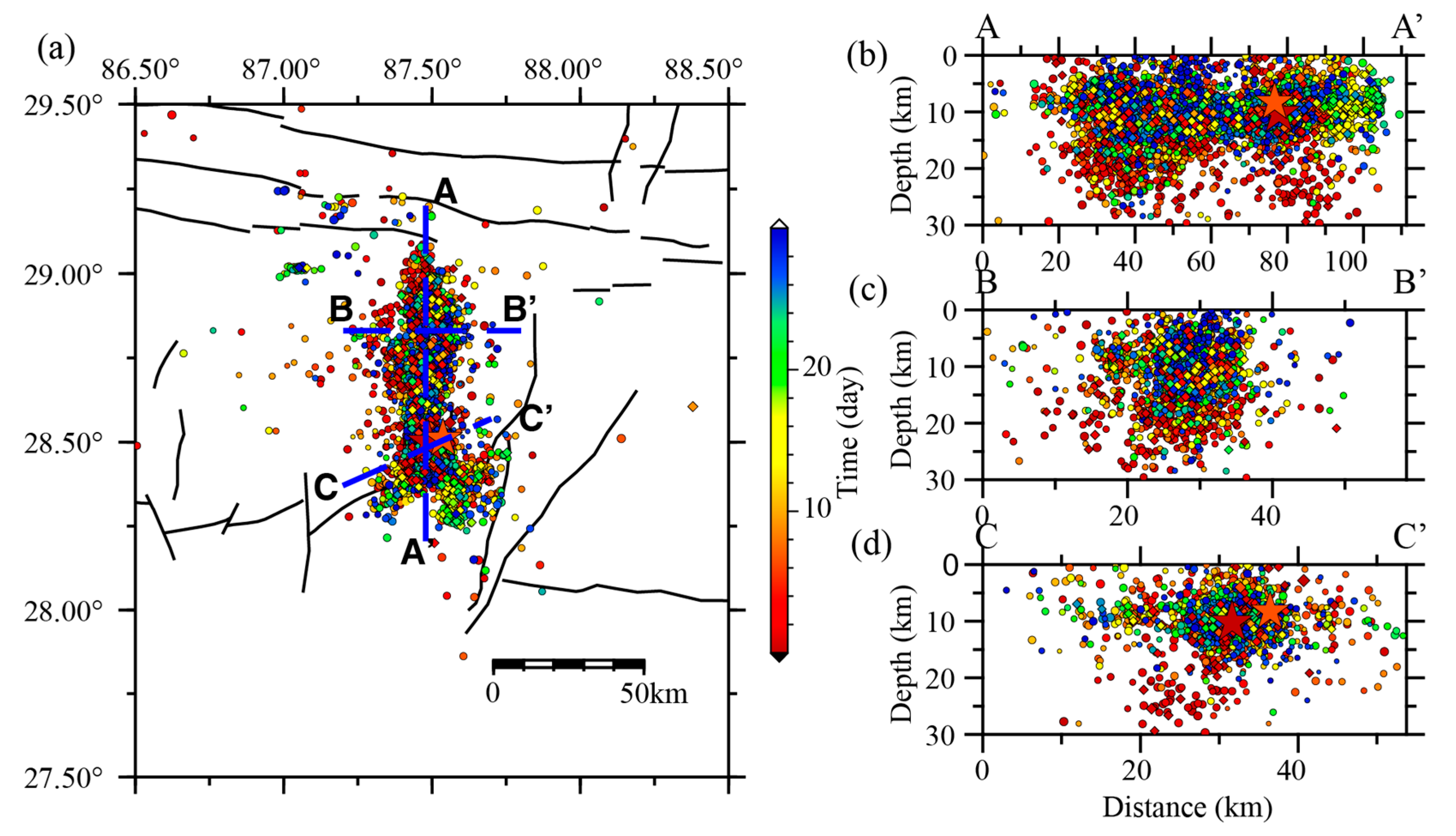
A total of 8942 earthquake hypocenters were obtained after relocation, and their spatial distribution is shown in Figure 3 and Figure 4. After relocation, the relocated epicenter of the Dingri M_wg 7.1 earthquake is located at (28.500° N, 87.488° E), with a focal depth of approximately 10.2 km. The seismic activity distribution prior to the Dingri M_wg 7.1 earthquake (Figure 4) shows that seismic events occurred in the northern part of the mainshock area toward the end of 2021, including a maximum magnitude event of M_wg 2.62 on 5 November 2021, at 09:48. Approximately one hour before the occurrence of the Dingri M_wg 7.1 earthquake, a noticeable foreshock sequence was observed near the mainshock epicenter, with the largest being an M_wg 2.71 earthquake at 08:52 on 5 January 2025.

The aftershock sequence of the Dingri M_wg 7.1 earthquake exhibits a “V”-shaped distribution, generally trending in a nearly north–south direction, with a total length of about 70 km. In terms of focal depth, the aftershocks are mainly concentrated between 3 km and 15 km. The aftershock sequence can be roughly divided into two segments—northern and southern—using Changsuo Township as the boundary. The mainshock is located in the southern segment, where the aftershocks trend predominantly in a northwest–northeast direction. Within this segment, a northeast-trending aftershock band is also present. On 13 January, the largest aftershock recorded so far (M_wg 3.71) occurred in this area. The northern segment of the aftershock sequence is characterized by a nearly north–south trend, with a northwest-trending branch located west of Changsuo Township. The spatial distribution of the relocated aftershocks indicates that the Dingri M_wg 7.1 earthquake involved a complex seismogenic structure (Figure 4). The depth cross-sections offer important evidence for interpreting the three-dimensional rupture geometry and fault structure. Along the A–A′ profile (Figure 4b), the aftershocks display a distinct “W-shaped” pattern, with two separate clusters located in the northern and southern segments and a clear seismicity gap near 28.6° N. This bimodal distribution suggests that the Dingri earthquake ruptured at least two discrete asperities or fault patches, rather than a single continuous fault plane. Such segmentation is typical of geometrically complex fault zones in regions of distributed deformation [43,44]. The gap between the two clusters may reflect a structural barrier—such as a step-over or bend—that temporarily halted rupture propagation, or a stronger, unbroken asperity that remains locked and may represent a future seismic hazard [45,46].

3.2. Spatiotemporal Variation in the b Value

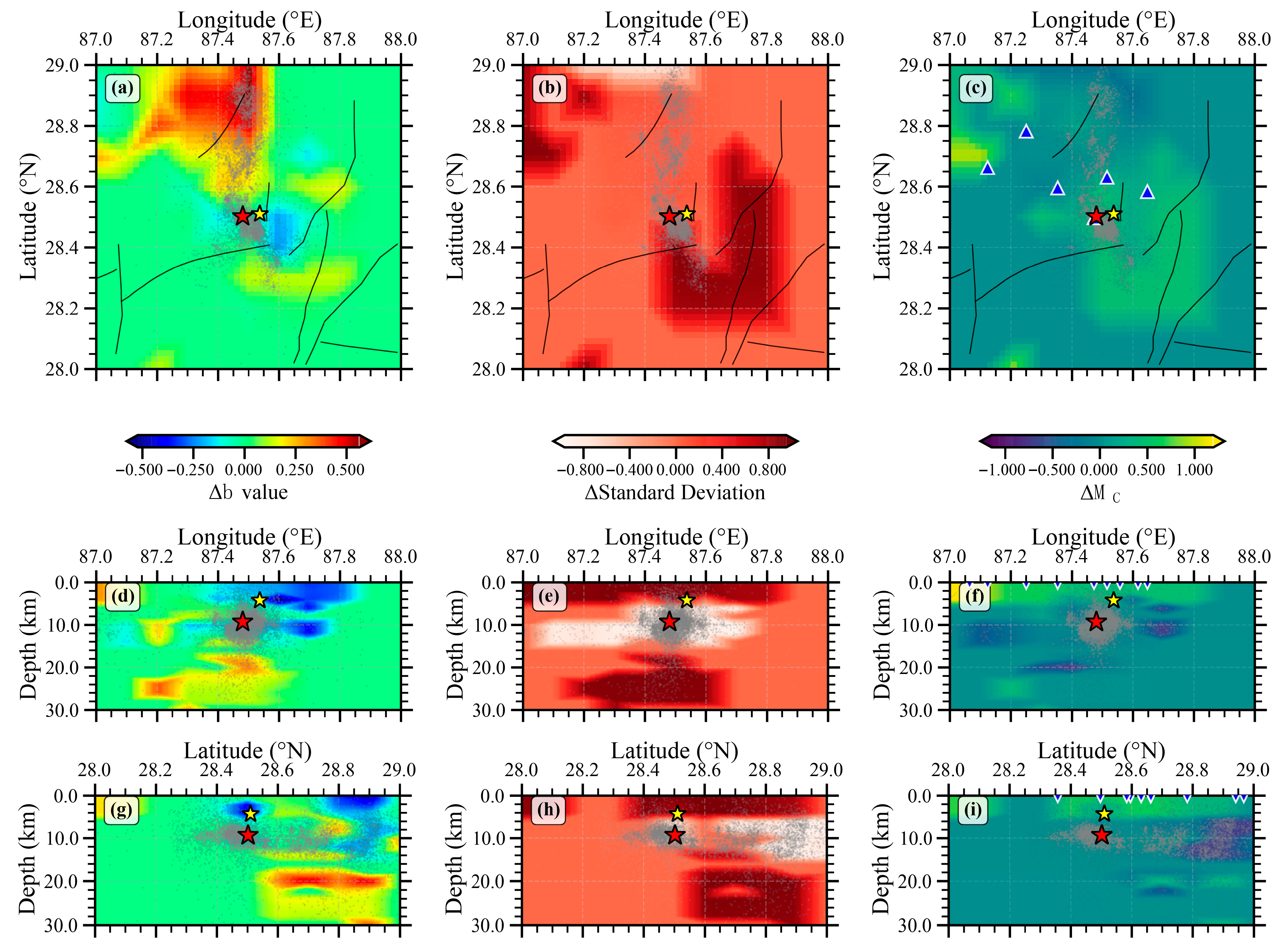
Comparison of b values between the two time windows reveals significant spatial variability in the Δb distribution across the study area (Figure 5a). Notably, the mainshock (marked by a red five-pointed star) and the largest aftershock (M_wg 3.71, marked by a yellow five-pointed star) are both located in areas where Δb decreased most significantly, by 0.25 to 0.3 units. The relative standard deviation of Δb across the entire Dingri Study Area, calculated in both horizontal and depth sections, ranges from −0.58 to 0.61. The variation in completeness magnitude M_C corresponds to a range of M_wg from −1.2 to +1.3. In particular, Figure 5g highlights a clear decrease in b values in the northern part of the mainshock zone (28.8–29.0° N). However, the horizontal map view shows a relatively smaller contrast, likely due to the influence of elevated b values at depths of 16–22 km on the overall surface representation.

3.3. Evolution of Seismic Interaction Networks

Having established the spatial and temporal patterns of stress accumulation through b value analysis, we now examine how the seismic interaction patterns evolved dynamically during the same periods. The Granger causality analysis revealed a significant temporal evolution in the complexity and spatial extent of the seismic interaction network across the three defined periods (Figure 6).

During the background period (2021–2023), the system exhibited a complex and widespread interaction network (Figure 6a). Among 32 active grid cells, a total of 73 statistically significant (p < 0.01) causal links were identified among 28 nodes. These interactions included numerous long-range connections spanning a broad area around the future epicenter, suggesting a period of extensive, system-wide stress adjustment.

In contrast, during the pre-mainshock period (2023–2025), the network underwent a notable simplification (Figure 6b). Although the number of active cells was comparable at 35, the number of significant (p < 0.01) causal links decreased by approximately 33% to 49 (among 34 nodes). The network became visibly sparser, with a marked reduction in long-range connections. This change indicates a shift from broad-scale interaction to a more localized process.

Following the mainshock, the aftershock period network, displayed an extremely simplified and localized pattern (Figure 6c). From 12 active cells, only 6 significant (p < 0.05) causal links were found among 7 nodes. These links are almost exclusively short-range and are tightly clustered along the north–south trending aftershock zone, demonstrating that post-rupture dynamics were governed purely by local stress redistribution.

4. Discussion

4.1. Spatiotemporal Evolution of b Values and Earthquake Occurrence

This study reveals a compelling spatial correlation between the distribution of Δb values and both the mainshock location and subsequent aftershock patterns. The b value near the mainshock decreased by approximately 0.5 units. This substantial reduction aligns remarkably well with precursory b value anomalies documented before other major earthquakes worldwide. Main et al. [47] demonstrated that b values typically fluctuate between 0.5 and 1.5 throughout an earthquake cycle, with critical rupture frequently initiating in regions where the b value approaches the lower bound of 0.5—a theoretical forecasting that closely matches our observations. Henderson et al. [48] further corroborated this pattern through their investigation of southern California seismicity, establishing that enhanced seismic activity preceding major earthquakes consistently correlates with anomalously low b values. These findings reinforce the interpretation that b value anomalies may serve as reliable indicators of stress accumulation approaching a critical threshold for rupture initiation.

Beyond the temporal evolution at the mainshock location, our analysis reveals a spatial correspondence between the Δb distribution and the subsequent aftershock zone geometry. The region exhibiting the most pronounced b value reduction (Δb > 0.5) extends approximately 40 km north of the mainshock epicenter—precisely where aftershock density reaches its maximum. This spatial correlation reflects the fundamental relationship between low b value regions and zones of elevated differential stress, where rupture propagation is mechanically favored [11]. The mainshock nucleated within the Shen’zha–Dingjie Normal Fault System, and the observed northward directivity of both the b value anomaly and aftershock distribution suggests strong structural control by the prevailing north–south extensional tectonic regime characteristic of this portion of the Tibetan Plateau [49,50,51]. Comparable spatial associations between pre-seismic b value minima and subsequent rupture zones have been documented in diverse tectonic settings, notably including the San Jacinto–Elsinore fault zone studied by Wyss et al. [9]. The consistency of these observations across different geological environments suggests that spatial b value mapping could provide valuable constraints for delineating potential rupture areas in seismic hazard assessments. The observed 26 km surface rupture length and its north–south orientation provide direct geological evidence supporting our interpretation of the b value anomaly distribution. The consistency between the geodetically observed co-seismic deformation field and the pre-seismic low b value zone further validates that these anomalies effectively delineated the area of maximum crustal strain accumulation prior to rupture [11].

The depth-resolved analysis reveals important vertical heterogeneity in the pre-seismic stress field. As shown in Figure 5d–i, the cross-sections exhibit a pronounced depth-dependent pattern: b values decrease markedly (Δb < −0.5) at shallow depths of 5–15 km, particularly in the northern region near 29°N where the mainshock hypocenter is located, while b values increase at depths greater than 20 km (positive Δb). This depth stratification suggests that elastic strain accumulated primarily within the brittle seismogenic layer (5–15 km), coinciding precisely with the depth distribution of the mainshock (10.2 km) and dense aftershock activity. The western portion of the study area (longitude 87.0–87.4° E) shows a consistent trend of b value reduction in the shallow crust, indicating westward extension of the stress concentration zone. The elevated b values at greater depths likely reflect either stress relaxation through ductile deformation in the lower crust or enhanced microseismicity in response to loading from the overlying locked asperity. Importantly, the horizontal map (Figure 5a) shows a relatively muted Δb pattern because depth-averaging incorporates the deeper high-b value signal, thereby masking the shallow stress anomaly. The latitude-depth sections (Figure 5g–i) most clearly reveal the spatial localization: the northern region exhibits the most dramatic b value changes concentrated at seismogenic depths, defining the three-dimensional geometry of the critically stressed fault patch that ultimately ruptured. This depth-confined stress concentration pattern demonstrates that b value mapping can effectively delineate not only the horizontal extent but also the vertical dimensions of impending rupture zones.

4.2. Dynamic Evolution of Seismic Interaction Networks

Complementing the quasi-static stress field revealed by b value analysis, the Granger causality network evolution provides crucial dynamic insights into how the seismogenic system responded to progressive stress loading. As detailed in Section 2.3, these networks represent statistical predictive relationships between seismic activity rates in different spatial regions. A causal link from region A to region B indicates that past earthquake counts in A significantly improve the prediction of current activity in B, potentially reflecting physical processes such as stress transfer or cascading fault interactions. During the background period (2021–2023), the system exhibited a remarkably complex interaction network comprising 73 statistically significant causal links among 28 active nodes. This highly interconnected state, characterized by numerous long-range correlations spanning the broader study area, likely represents a phase of distributed stress adjustment across a mechanically heterogeneous and pervasively fractured crustal volume. In practical terms, this means that seismic activity in one grid cell was statistically useful for predicting activity in many other cells across the region. The existence of these widespread predictive relationships suggests that the seismogenic system was in a state of broad mechanical coupling, where stress perturbations in one location could influence seismicity patterns throughout the study area. This distributed interaction pattern is consistent with a crust undergoing regional tectonic adjustment prior to strain localization. As the system transitioned into the pre-mainshock period (2023–2025), however, the network underwent a dramatic simplification, with significant causal links decreasing by approximately 33% to only 49 connections among 34 nodes. Critically, this reduction occurred while the number of seismically active grid cells remained comparable (28 vs. 34), meaning fewer cells were successfully predicting each other’s behavior despite similar overall activity levels. This progressive loss of long-range correlations—where distant regions that previously showed statistical coupling became predictively independent—indicates a fundamental reorganization of the system’s internal dynamics. In seismological terms, the predictive utility of distant seismicity diminished, suggesting that local stress states were becoming increasingly determined by local processes rather than regional interactions. Such transitions, where complex systems exhibit reduced internal correlations as they approach critical points, constitute a well-documented phenomenon in statistical physics, often manifested as critical slowing down or loss of fluctuation–dissipation relationships [48].

4.3. Physical Interpretation: From System-Wide Adjustment to Pre-Failure Lock-In

The spatiotemporal correlation between b value evolution and network simplification—both in their temporal progression and spatial localization—points toward a unified physical mechanism governing both observations: the emergence of a “locked-in” state as the fault system approaches catastrophic failure. Quantitatively, the pre-mainshock period (2023–2025) witnessed a dramatic b value drop about 0.5 in the epicentral region. Spatially, both anomalies concentrated in the same northward corridor (28.8–29.0° N) that would subsequently host the densest aftershock activity. This dual convergence—temporal and spatial—is unlikely to be coincidental. Rather, it suggests that b value analysis and Granger causality networks capture complementary aspects of the same underlying preparatory process. While the b value provides a quasi-static “snapshot” of the regional stress state at each time period, the Granger network reveals how the system dynamically arrived at that state through evolving patterns of stress transfer and seismic interaction. Together, they trace the complete trajectory from distributed loading to localized failure. We interpret this state as representing the terminal phase of stress concentration onto the primary asperity that would ultimately host the mainshock nucleation. As tectonic loading progressively focuses stress onto this mechanically competent but critically loaded fault patch, its effective stiffness increases while its sensitivity to external perturbations diminishes. This mechanical evolution naturally explains the observed severing of long-range interaction pathways—the incipient rupture zone becomes increasingly isolated from the surrounding stress field, responding primarily to local rather than regional stress fluctuations. This interpretation finds strong support in theoretical models of earthquake nucleation, which forecast that fault zones approaching failure should exhibit both decreasing b values (reflecting stress concentration) and reduced triggering susceptibility (reflecting mechanical isolation) [47].

Connecting statistical patterns to physical processes: It is important to emphasize how the observed network evolution translates to physical understanding. The Granger causality test identifies whether the temporal pattern of earthquakes in region A helps predict earthquakes in region B. During the background period, such predictive relationships were abundant and far-reaching, suggesting that stress perturbations propagated broadly through the seismogenic system. As the system approached failure, these long-range predictive links systematically disappeared. We interpret this as the mechanical decoupling of the incipient rupture zone: as stress concentrated onto the primary asperity, it became increasingly “blind” to distant stress changes and increasingly dominated by local mechanics. The aftershock network, with only 7 local links, confirms this interpretation—post-rupture stress redistribution is purely local, as expected from elastic rebound theory.

This interpretation is further validated by the spatial correlation between network changes and b value anomalies (Figure 5). The regions showing the strongest b value decline (Δb > 0.5, indicating stress concentration) largely coincide with the nodes that lost long-range connections in the network analysis. This convergence of two independent statistical approaches—one measuring magnitude distributions, the other measuring temporal correlations—toward the same spatial pattern of pre-seismic anomaly provides robust evidence that we are observing a real, systematic physical process rather than statistical artifacts.

4.4. Integrated Validation Through Aftershock Sequence Analysis

The aftershock sequence analysis provides corroborating evidence of this integrated interpretation. Following the mainshock, the interaction network collapsed to an extremely sparse configuration comprising merely 6 significant links among 7 nodes, all tightly confined to the primary rupture zone. This represents an order-of-magnitude reduction from the pre-mainshock network complexity, confirming that the mainshock effectively released the accumulated regional stress that had been driving system-wide interactions. The post-rupture dynamics became overwhelmingly local, governed exclusively by stress redistribution along and adjacent to the primary fault plane. This evolutionary sequence—from complex distributed interactions during regional loading, through simplified “locked-in” dynamics during final approach to failure, to purely local relaxation following rupture—provides a coherent narrative of the complete earthquake cycle. The dual-perspective analysis presented here, integrating static stress indicators with dynamic system behavior, thus offers a more comprehensive framework for understanding the mechanical processes governing large earthquake occurrence. This approach may prove particularly valuable for identifying future earthquakes that exhibit similar precursory patterns, potentially enhancing our capacity for time-dependent seismic hazard assessment.

5. Conclusions

This study provides a comprehensive analysis of pre-seismic activity and stress dynamics associated with the M_wg 7.1 Dingri earthquake in Tibet on 7 January 2025, revealing significant spatiotemporal variations in b values and their correlation with aftershock distribution and seismic interaction networks.

Our key findings demonstrate that the most significant b value reduction (Δb > 0.5) occurred north of the mainshock epicenter, spatially coinciding with dense aftershock clustering. This pattern suggests that elevated differential stress in this region facilitated focused rupture propagation during the mainshock. Granger causality analysis reveals a systematic evolution of seismic interactions across three distinct phases: (i) a complex background network with 73 causal links (2021–2023), (ii) a transitional pre-mainshock network with 49 links (2023–2025) indicating progressive stress localization, and (iii) a highly simplified post-mainshock network with only 6 links, reflecting the transition from system-wide stress adjustment to a “locked-in” state and subsequent local stress relaxation. The integration of b value anomalies with seismic interaction network evolution provides a robust framework for understanding earthquake nucleation processes, offering valuable insights for seismic hazard assessment in the Tibetan Plateau and analogous tectonic settings.

The application of VAR models to inherently non-stationary aftershock sequences requires careful interpretation. Although first-order differencing was applied to mitigate the dominant temporal decay trend, ADF tests revealed that stationarity was achieved for the majority, but not all, of active time series. This residual non-stationarity in some series—likely attributable to the limited temporal window and complex aftershock dynamics—indicates that our VAR model may not capture the complete spectrum of seismic interactions. Consequently, the post-mainshock interaction network should be interpreted as indicative of dominant causality patterns rather than an exhaustive representation of all physical interactions. Future studies incorporating longer observation periods and advanced non-stationary time series methods could further refine these interaction networks.

References

1. Ishimoto, M. Observation of Earthquakes Registered with the Microseissmograph Constructed Recently (I). Bull. Earthq. Res. Inst. Univ. Tokyo 1939, 17, 443. [Google Scholar]
2. Gutenberg, B.; Richter, C. Seismicity of the Earth and Associated Phenomena; Princeton University Press: Princeton, NJ, USA, 1954; ISBN 0-598-97720-1. [Google Scholar]
3. Lay, T.; Wallace, T.C. Modern Global Seismology; Elsevier: Amsterdam, The Netherlands, 1995; Volume 58, ISBN 0-08-053671-9. [Google Scholar]
4. Ogata, Y.; Katsura, K. Analysis of Temporal and Spatial Heterogeneity of Magnitude Frequency Distribution Inferred from Earthquake Catalogues. Geophys. J. Int. 1993, 113, 727–738. [Google Scholar] [CrossRef]
5. Schorlemmer, D.; Wiemer, S.; Wyss, M. Earthquake Statistics at Parkfield: 1. Stationarity of b Values. J. Geophys. Res. Solid Earth 2004, 109, B12307. [Google Scholar] [CrossRef]
6. Sanchez, J.J.; McNutt, S.R.; Power, J.A.; Wyss, M. Spatial Variations in the Frequency-Magnitude Distribution of Earthquakes at Mount Pinatubo Volcano. Bull. Seismol. Soc. Am. 2004, 94, 430–438. [Google Scholar] [CrossRef]
7. Wiemer, S.; McNutt, S.R. Variations in the Frequency-magnitude Distribution with Depth in Two Volcanic Areas: Mount St. Helens, Washington, and Mt. Spurr, Alaska. Geophys. Res. Lett. 1997, 24, 189–192. [Google Scholar] [CrossRef]
8. Wyss, M.; Stefansson, R. Nucleation Points of Recent Mainshocks in Southern Iceland, Mapped by b values. Bull. Seismol. Soc. Am. 2006, 96, 599–608. [Google Scholar] [CrossRef]
9. Wyss, M.; Schorlemmer, D.; Wiemer, S. Mapping Asperities by Minima of Local Recurrence Time: San Jacinto-Elsinore Fault Zones. J. Geophys. Res. Solid Earth 2000, 105, 7829–7844. [Google Scholar] [CrossRef]
10. Smith, W.D. The b-Value as an Earthquake Precursor. Nature 1981, 289, 136–139. [Google Scholar] [CrossRef]
11. Schorlemmer, D.; Wiemer, S.; Wyss, M. Variations in Earthquake-Size Distribution across Different Stress Regimes. Nature 2005, 437, 539–542. [Google Scholar] [CrossRef] [PubMed]
12. Jiang, C.; Jiang, C.; Yin, F.; Zhang, Y.; Bi, J.; Long, F.; Si, Z.; Yin, X. A New Method for Calculating B-Value of Time Sequence Based on Data-Driven (TbDD): A Case Study of the 2021 Yangbi MS 6.4 Earthquake Sequence in Yunnan. Chin. J. Geophys. 2021, 64, 3126–3134. (In Chinese) [Google Scholar]
13. Yin, F.; Jiang, C. Enhanced B-Value Time-Series Calculation Method Using Data-Driven Approach. Geophys. J. Int. 2024, 236, 78–87. [Google Scholar] [CrossRef]
14. Xu, X.; Wang, S.; Cheng, J.; Wu, X. Shaking the Tibetan Plateau: Insights from the MW 7.1 Dingri earthquake and its implications for active fault mapping and disaster mitigation. NPJ Nat. Hazards 2025, 2, 16. [Google Scholar] [CrossRef]
15. Yin, X.; Zhang, X.; Cai, R.; Wang, H.; Liu, F. Fast 1-D Velocity Optimization Inversion to 3D Velocity Imaging: A Case Study of Sichuan Maerkang Earthquake Swarm in 2022. Sustainability 2022, 14, 15909. [Google Scholar] [CrossRef]
16. Scholz, C.H. On the stress dependence of the earthquake b value. Geophys. Res. Lett. 2015, 42, 1399–1402. [Google Scholar] [CrossRef]
17. Goebel, T.H.W.; Schorlemmer, D.; Becker, T.W.; Dresen, G.; Sammis, C.G. Acoustic emissions document stress changes over many seismic cycles in stick-slip experiments. Geophys. Res. Lett. 2017, 44, 2967–2974. [Google Scholar] [CrossRef]
18. Bi, J.; Cao, F.; Ma, Y. Seismicity characteristics based on the spatiotemporal ETAS model in North China from the perspective of different cut-off magnitude. PLoS ONE 2025, 20, e0327295. [Google Scholar] [CrossRef]
19. Yin, X.; Jiang, C.; Yin, F.; Zhai, H.; Zheng, Y.; Wu, H.; Liu, X.; Li, J. Assessment and optimization of maximum magnitude forecasting models for induced seismicity in enhanced geothermal systems: The Gonghe EGS project in Qinghai, China. Tectonophysics 2024, 886, 230438. [Google Scholar] [CrossRef]
20. Granger, C.W. Investigating Causal Relations by Econometric Models and Cross-Spectral Methods. Econom. J. Econom. Soc. 1969, 37, 424–438. [Google Scholar] [CrossRef]
21. Waldhauser, F.; Ellsworth, W.L. A Double-Difference Earthquake Location Algorithm: Method and Application to the Northern Hayward Fault, California. Bull. Seismol. Soc. Am. 2000, 90, 1353–1368. [Google Scholar] [CrossRef]
22. Cai, M.; Chen, J.; Yin, X. Three-dimensional velocity structure and relocation of earthquakes in Luding area, Sichuan Province. China Earthq. Eng. J. 2023, 45, 552–564. (In Chinese) [Google Scholar]
23. Yin, X.; Wang, S.; Liang, X.; Ma, G. Impact of fault complexity on aftershock decay: A case study of the Wushi MS 7.1 earthquake. China Earthq. Eng. J. 2024, 46, 965–972+991. (In Chinese) [Google Scholar]
24. Xin, H.; Zhang, H.; Kang, M.; He, R.; Gao, L.; Gao, J. High-resolution Lithospheric Velocity Structure of Continental China by Double-difference Seismic Travel-time Tomography. Seismol. Res. Lett. 2019, 90, 229–241. [Google Scholar] [CrossRef]
25. China Earthquake Administration. Earthquake Cataloging Specifications (DB/T 66-2016); Seismological Press: Beijing, China, 2016. (In Chinese) [Google Scholar]
26. Purcaru, G.; Berckhemer, H. A magnitude scale for very large earthquakes. Tectonophysics 1978, 49, 189–198. [Google Scholar] [CrossRef]
27. Hanks, T.C.; Kanamori, H. A moment magnitude scale. J. Geophys. Res. 1979, 84, 2348–2350. [Google Scholar] [CrossRef]
28. Das, A.; Das, T.; Chaudhuri, C.H.; Choudhury, D. Integrated study on buried pipelines, co-seismic landslides, and magnitude conversion for 2023 Türkiye earthquake. Eng. Geol. 2024, 337, 107599. [Google Scholar] [CrossRef]
29. Thatcher, W.; Hanks, T.C. Source parameters of southern California earthquakes. J. Geophys. Res. 1973, 78, 8547–8576. [Google Scholar] [CrossRef]
30. Hutton, L.K.; Boore, D.M. The ML scale in southern California. Bull. Seismol. Soc. Am. 1987, 77, 2074–2094. [Google Scholar] [CrossRef]
31. Choy, G.L.; Boatwright, J.L. Global patterns of radiated seismic energy and apparent stress. J. Geophys. Res. 1995, 100, 18205–18228. [Google Scholar] [CrossRef]
32. Ristau, J.; Rogers, G.C.; Cassidy, J.F. Moment magnitude-local magnitude calibration for earthquakes in western Canada. Bull. Seismol. Soc. Am. 2003, 93, 2994–3000. [Google Scholar] [CrossRef]
33. Keir, D.; Hamling, I.J.; Ayele, A.; Calais, E.; Ebinger, C.; Wright, T.J.; Jacques, E.; Mohamed, K.; Hammond, J.O.; Belachew, M. Evidence for focused magmatic accretion at segment centers from lateral dike injections captured beneath the Red Sea rift in Afar. Geology 2009, 37, 59–62. [Google Scholar] [CrossRef]
34. Kanamori, H. The energy release in great earthquakes. J. Geophys. Res. 1977, 82, 2981–2987. [Google Scholar] [CrossRef]
35. Das, R.; Sharma, M.L.; Wason, H.R.; Choudhury, D.; Gonzalez, G. A seismic moment magnitude scale. Bull. Seismol. Soc. Am. 2019, 109, 1542–1555. [Google Scholar] [CrossRef]
36. Kanamori, H. Magnitude scale and quantification of earthquakes. Tectonophysics 1983, 93, 185–199. [Google Scholar] [CrossRef]
37. Gutenberg, B.; Richter, C.F. Magnitude and energy of earthquakes. Nature 1955, 176, 795. [Google Scholar] [CrossRef]
38. Mignan, A.; Woessner, J. Estimating the Magnitude of Completeness for Earthquake Catalogs. Community Online Resour. Stat. Seism. Anal. 2012, 1–45. [Google Scholar] [CrossRef]
39. Woessner, J.; Wiemer, S. Assessing the Quality of Earthquake Catalogues: Estimating the Magnitude of Completeness and Its Uncertainty. Bull. Seismol. Soc. Am. 2005, 95, 684–698. [Google Scholar] [CrossRef]
40. Ak, K. Maximum likelihood estimate of b in the formula log N = a-bM and its confidence limits. Bull. Earthquake Res. Inst. Tokyo Univ. 1965, 43, 237–239. [Google Scholar]
41. Bengoubou-Valerius, M.; Gibert, D. Bootstrap determination of the reliability of b values: An assessment of statistical estimators with synthetic magnitude series. Nat. Hazards 2013, 65, 443–459. [Google Scholar] [CrossRef]
42. Engle, R.F.; Granger, C.W.J. Co-integration and error correction: Representation, estimation, and testing. Econometrica 1987, 55, 251–276. [Google Scholar] [CrossRef]
43. Huang, M.H.; Fielding, E.J.; Liang, C.; Milillo, P.; Bekaert, D.; Dreger, D.; Salzer, J. Coseismic deformation and triggered landslides of the 2016 Mw 6.2 Amatrice earthquake in Italy. Geophys. Res. Lett. 2017, 44, 1266–1274. [Google Scholar] [CrossRef]
44. Elliott, J.R.; Walters, R.J.; England, P.C.; Jackson, J.A.; Li, Z.; Parsons, B. Extension on the Tibetan plateau: Recent normal faulting measured by InSAR and body wave seismology. Geophys. J. Int. 2010, 183, 503–535. [Google Scholar] [CrossRef]
45. King, G.; Nábělek, J. Role of fault bends in the initiation and termination of earthquake rupture. Science 1985, 228, 984–987. [Google Scholar] [CrossRef]
46. Wesnousky, S.G. Predicting the endpoints of earthquake ruptures. Nature 2006, 444, 358–360. [Google Scholar] [CrossRef] [PubMed]
47. Main, I.G.; Meredith, P.G.; Jones, C. A Reinterpretation of the Precursory Seismic b Value Anomaly from Fracture Mechanics. Geophys. J. Int. 1989, 96, 131–138. [Google Scholar] [CrossRef]
48. Henderson, J.; Main, I.G.; Pearce, R.G.; Takeya, M. Seismicity in North-Eastern Brazil: Fractal Clustering and the Evolution of the b Value. Geophys. J. Int. 1994, 116, 217–226. [Google Scholar] [CrossRef]
49. Scheffer, M.; Bascompte, J.; Brock, W.A.; Brovkin, V.; Carpenter, S.R.; Dakos, V.; Held, H.; Van Nes, E.H.; Rietkerk, M.; Sugihara, G. Early-Warning Signals for Critical Transitions. Nature 2009, 461, 53–59. [Google Scholar] [CrossRef]
50. Qiao, X.; Lu, Z.; Yan, S.; Shi, H.; Zhi, M.; Zhao, D. The 2025 MW 7.0 Dingri Earthquake: Conjugate Normal Faulting of a Graben Structure in the Southern Xainza-Dinggye Rift. Geophys. Res. Lett. 2025, 52, e2025GL116154. [Google Scholar] [CrossRef]
51. Yu, S.; Zhang, S.; Luo, J.; Li, Z.; Ding, J. The Tectonic Significance of the MW 7.1 Earthquake Source Model in Tibet in 2025 Constrained by InSAR Data. Remote Sens. 2025, 17, 936. [Google Scholar] [CrossRef]
Figure 1. Structural background, station distribution, and temporal evolution of seismicity prior to the Mwg 7.1 Dingri earthquake. The map shows the spatial distribution of earthquakes across three distinct temporal periods: background seismicity (2021–2023, light blue circles), pre-mainshock seismicity (2023–2025, orange circles), and foreshock sequence (7 January 2025, red circles). Circle sizes are proportional to earthquake magnitude. The yellow star marks the Mwg 7.1 Dingri mainshock epicenter. Blue triangles represent permanent seismic stations, while dark red triangles show temporary monitoring stations deployed on 9 January 2025. Black lines denote major fault traces.
Applsci 15 11685 g001
Figure 2. Travel-time curves for P and S waves. The red dots represent the travel-time data of seismic phases used for precise relocation. Panel (a) shows the P-wave travel-time curve. Panel (b) shows the S-wave travel-time curve.
Applsci 15 11685 g002
Figure 3. Seismic activity distribution before and after the Mwg 7.1 Dingri earthquake. Red star represent the mainshock. (a) Distribution of seismicity during the background and pre-mainshock periods (2021–2025). The foreshock sequence occurring approximately one hour before the mainshock is highlighted within the blue dashed rectangle, with the largest foreshock (Mwg 2.71) marked by a blue star. Earthquakes are colored by time (in days) since 7 January 2021, using a GMT seis colormap. The diamonds indicate earthquake events with magnitude Mwg ≥ 0.63. (b) Aftershock density distribution within 30 days following the mainshock, showing a prominent north–south trending pattern extending approximately 70 km. The largest aftershock (Mwg 3.71) that occurred on 13 January 2025, is marked by a yellow star. In both panels, the red star denotes the Mwg 7.1 mainshock epicenter, black lines represent faults, and circles indicate cities. The color bars indicate time (days) for panel (a) and aftershock density for panel (b).
Applsci 15 11685 g003
Figure 4. Three-dimensional spatial distribution of relocated aftershocks following the Mwg 7.1 Dingri earthquake, revealing complex fault geometry and seismogenic structure. In the figure, different colors represent the occurrence times of earthquakes, and the black lines represent fault lines. (a) Map view showing the “V-shaped” aftershock pattern with distinct northern and southern segments separated by Changsuo Township (marked location). The northern segment exhibits a predominant N-S trend, while the southern segment (containing the mainshock) shows NW-NE orientation. Red star: Mwg 7.1 mainshock epicenter; Yellow star: Mwg 3.71 largest aftershock (13 January 2025). (bd) Depth cross-sections along profiles A-A’, B-B’, and C-C’ (locations shown in panel a), illustrating the vertical distribution of aftershocks primarily concentrated between 3 and 15 km depth, corresponding to the seismogenic layer within the brittle upper crust. The dense clustering along specific depth ranges indicates strong mechanical stratification of the fault zone. Color scale represents time since mainshock (in days), revealing the spatiotemporal evolution of the aftershock sequence.
Applsci 15 11685 g004
Figure 5. Spatial distribution of Δb values in the Dingri study area. The blue triangles represent seismic stations. Panels (a,d,g) show the b value distribution in the horizontal plane, longitude–depth section, and latitude–depth section, respectively. Panels (b,e,h) display the standard deviation distribution. Panels (c,f,i) present the spatial distribution of MC. Red star denotes the Mwg 7.1 Dingri earthquake; yellow star indicates the Mwg 3.71 aftershock that occurred on 13 January 2025. Background seismicity (gray dots) shows all relocated aftershocks (Panels (ac)), and seismic stations are marked by triangles (Panels (c,f,i)).
Applsci 15 11685 g005
Figure 6. Granger causality networks showing the evolution of seismic interactions. Red arrows indicate statistically significant causal relationships. The green dots represent unassociated earthquakes, while the other colors correspond to associated earthquakes from different time periods. (a) The complex and widespread network during the background period (2021–2023), with 73 links identified at a p-value threshold of 0.01. (b) The simplified network during the pre-mainshock period (2023–2025), with 49 links (p < 0.01). (c) The highly sparse and localized network during the aftershock sequence, with only 6 links identified among 7 nodes at a p-value threshold of 0.05.
Applsci 15 11685 g006
Disclaimer/Publisher’s Note: The statements, opinions and data contained in all publications are solely those of the individual author(s) and contributor(s) and not of MDPI and/or the editor(s). MDPI and/or the editor(s) disclaim responsibility for any injury to people or property resulting from any ideas, methods, instructions or products referred to in the content.