Predicting the Cooling Rate in Steel-Part Heat Treatment via Random Forests

Abstract

Heat treatment is a thermal-processing method involving controlled heating and cooling cycles designed to achieve the desired properties of materials. Among these steps, the cooling rate in heat treatment plays a crucial role, as it significantly influences the resulting material properties. In this paper, we investigated the feasibility of random forests in estimating the cooling-rate parameters for the steel-part heat treatment process. Random forests are particularly appealing in modeling an ensemble of expressive decision trees from which cooling can be modeled and estimated from the interaction of metal features. Our computational experiments using real-world data from industrial-scale operations demonstrated the advantageous properties of random forest regression models, particularly when combined with a random oversampling scheme. We also found that the chemical composition—specifically carbon and chromium content—as well as the weight of the steel parts, are key features that predict the cooling rate of steel parts. Furthermore, our validation using real-world cooling scenarios aligned closely with the practical insights of seasoned operators who routinely recommend cooling parameters for the metal-normalizing process. Our results highlight the effectiveness of the ensemble approach of random forest for practical applicability in industrial-scale heat treatment.

1. Introduction

Iron-steel metals are widely used in construction and structural applications, as well as in consumer products involving machines, cars, gears, shafts, bolts, and axles. Heat treatment is advantageous for metals by inducing phase changes and by modifying mechanical properties such as hardness, toughness, impact resistance, ductility, and corrosion resistance. Heat treatment is a thermal processing technique that tunes the microstructure of metals by subjecting them to controlled heating and cooling cycles, often without changing the overall shape. Heat treatment parameters such as the heating temperature, the holding time, and the cooling rate determine the final mechanical properties of metals. As such, different combinations of heat-treatment parameters can lead to a diverse set of mechanical properties.

The Heat treatment of iron-steel metals is often conducted in carbon-emitting heating furnaces [1]. Such steel parts are placed on trays and heated to a desired temperature (often above 900 °C) and then cooled in the furnace (annealing), in air (normalizing), or in water/oil (hardening), depending on the desired target properties [2]. Annealing cools metals slowly and produces soft, ductile, and workable properties. In contrast, hardening involves faster cooling, resulting in metals that are hard and strong but brittle. Normalizing falls between these two processes, with moderate cooling that produces balanced mechanical properties [2].

The cooling rate during the heat treatment of metals allows for tuning the type, size, and distribution of precipitates, thereby determining a balance between strength—when precipitates are fine and densely or evenly distributed to impede dislocation motion—and ductility, when precipitates are spaced, allowing for plastic deformation [3]. Concomitant with the above, the cooling rate in heat treatment determines the width of layers in layered structures [4], the width of lamellar structures within grains [5], the refinement of coarse, fully lamellar microstructures [6], the extent of continuous layers in grain boundaries [5], the precipitate formation (e.g., boundary vs. intragranular) and changes in the fracture mechanism (e.g., intergranular cracking vs. transgranular cracking) [7], the spacing between dendrites—the tree-like crystal structures that form when a metal cools [8], the grain boundaries, and the generation of dislocation sites in accordance with the Hall–Petch effect [9,10,11], the growth and distribution of austenite and corrosion resistance [12], the magnetic permeability of amorphous magnetic alloys [13], the dislocation density and microstrain formation [14], and the kinetics of atomic nucleation–diffusion in phase transformations [15].

Estimating the quantitative relationship between the cooling rate after heat exposure and the resulting microstructure in metal alloys has attracted significant attention in the manufacturing community due to its practical benefits. It is known that the microstructural properties of metals are influenced by both cooling rates and chemical compositions [16,17,18,19], yet the relationships are known to be nonlinear, making them well suited for machine learning and data-based approaches. Li et al. [20] predicted intermetallic morphology in recycled Al-Si-Cu alloys using machine learning based on cooling rates and chemical compositions. Gao et al. [18] established an exponential relationship between the critical cooling rate in U75V rail steel and its chemical composition, specifically based on carbon (C), manganese (Mn), silicon (Si), and vanadium (V). Geng et al. [21] found that not only cooling time but also chemical composition—specifically carbon (C), molybdenum (Mo), manganese (Mn), and nickel (Ni)—determined the hardness of low-alloy steel in welding applications. Afflerbach et al. [22] used features of the constituent chemical elements of bulk metallic glasses to predict the critical cooling rate for glass formation. Schultz et al. [23] used calculated features derived from chemical elements and molecular properties to predict the critical cooling rate of metallic glasses. Mehmet Akif Koç et al. [24] used neural networks to forecast cooling rates based on pressure, distance to sections, and the duration throughout H-section profiles of steel beams S275/HEA120, S275/HEB120, and S275/HEB14. Liu et al. [25] proposed an equation to predict the critical cooling rate of U71Mn rail steel as a function of holding temperatures and austenitizing times, both of which are key parameters determining the microstructure and stability of austenite.

Rapid cooling rates refine metal microstructures, suppress atomic diffusion, reduce micropores and grain sizes, and lead to a homogeneous distribution of precipitates and higher corrosion resistance. However, too-rapid cooling may result in brittle microstructures, making metals prone to cracking and fracture; therefore, the strength of each metal alloy must be carefully controlled. Although the above-mentioned studies explored the relationships between cooling rates and chemical composition and other mechanical notions involved in heat treatment of metals, the applicability to different metal alloys’ being relevant to industrial-scale operations remains unclear. If a pragmatic approach were considered, it would be desirable to elucidate whether geometry, weight, and material play as significant a role as chemical composition in predicting the cooling rate of the heat treatment of industrial-scale iron-steel parts. This question has remained elusive in the related works. As such, we aim to forecast the cooling rate for industrial-scale steel parts involved in the operations of Tsukimi Factory of Nagato Co., Ltd. (Hiroshima, Japan), an industrial plant that operates furnaces and cooling devices for the heat treatment of steel parts. In this setting, heat treatment is performed using specialized equipment (heating furnaces), and steel parts are heated in trays and then cooled using air via a cooling fan, as shown in Figure 1, or by immersing them in oil. Heat-treatment parameters such as heating temperatures and cooling rates are entered by the operator, with the cooling rate typically set based on the results of past, similar steel parts, and the intuition of experienced operators. This practice often leads to issues with personalization, accuracy, and repeatability.

In this paper, to tackle the aforementioned, we investigate the feasibility of regression and classification models aided via the ensemble approach of random forests [26,27]. Our goal is to model decision trees that predict the cooling rate parameter based on features such as chemical composition, material type, weight, and the geometry of industrial-scale iron-steel parts—information that is solely obtained for each part from daily plant operations. Additionally, we aim to analyze feature importance when decision trees successfully predict the cooling rate. Our computational experiments demonstrate the merits of regression-based random forest models, particularly when combined with an oversampling scheme. Furthermore, our validation using real-world cooling scenarios shows that the cooling parameters recommended through the random forest model consistently produced steel parts whose hardenability was within the standard acceptable range. Our findings highlight the practical merits of random forests for predicting cooling rates in the normalization of industrial-scale steel parts.

Of the following sections, Section 2 explains the learning mechanism of the random forest algorithm [26,27], Section 3 presents our computational experiments and results, and Section 4 concludes the study by summarizing the key findings.

2. Random Forest

In this section, we describe the key algorithm involved in constructing the trees within random forests. Let the training dataset be denoted as $X=\{x_0,x_1,\dots ,x_{n-1}\}$, where n is the total number of samples in the dataset, and let $y=\{y_0,y_1,\dots ,y_{n-1}\}$ be the associated target values. Our goal is to find a tree-based mapping function, $\tau :X\to y$. In what follows, we review the major components of the random forest implementation from scikit-learn [26,27], which constructs the function $\tau$ from a collection of trees (also known as a forest).

2.1. Bootstrap Sample

Each tree, $\mathcal{T}$, in a random forest in scikit-learn [26,27] is trained on a bootstrap sample, $X^{*}$, a subset of X, constructed as $X^{*}=\{x_{u_0},x_{u_1},\dots ,x_{u_{k-1}}\}$ and $y^{*}=\{y_{u_0},y_{u_1},\dots ,y_{u_{k-1}}\}$, where $u_i\in [0,n-1]$, $i\in [0,k-1]$, denotes the index of the selected sample. The bootstrap sample $X^{*}$ is constructed as follows: m sample indices $I_0,I_1,\dots ,I_{m-1}$ are generated; each $I_j\in [0,n-1]$ is drawn independently and uniformly at random (sampling with replacement):

$$I_j\sim \mathrm{Uniform}(0,n-1),j=0,\dots ,m-1.$$

As such, the set $U=\{u_0,u_1,\dots ,u_{k-1}\}=\{I_j:j=0,\dots ,m-1\}$ corresponds to unique (non-repeating) indices associated with the bootstrap samples: $x_{u_0},x_{u_1},\dots ,x_{u_{k-1}}$. Then, for each $i=0,\dots ,k-1$, the sample weight $w_i$ is the count of the samples of the generated indices:

$$w_i=\sum _{j=0}^{m-1}{\mathbf{1}}_{\{I_j=u_i\}}\mathrm{where}{\mathbf{1}}_{\{I_j=u_i\}}=\left\{\begin{array}{cc}1\hfill & \mathrm{if}{I}_j=u_i,\hfill \\ 0\hfill & \mathrm{otherwise}.\hfill \end{array}\right.$$

(1)

The above aims to randomly select (with replacement) k samples from the original dataset, in which samples picked multiple times get a higher weight and are to fit more closely than lower-weight samples. The above-mentioned mechanism extends Breiman’s original bootstrap sampling mechanism [28] and bagging (bootstrap aggregating) [29] to learn multiple versions of trees on bootstrap subsets of the training (learning) set.

2.2. Tree Construction

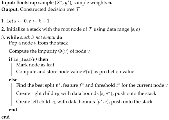
The tree construction algorithm in random forests follows a depth-first, stack-based routine (Algorithm 1) by default [26,27]; the inputs to the algorithm are the bootstrap sample $X^{*}=\{x_{u_0},x_{u_1},\dots ,x_{u_{k-1}}\}$, target $y^{*}=\{y_{u_0},y_{u_1},\dots ,y_{u_{k-1}}\}$, and its associated sample weights, $\mathit{w}=(w_0,w_1,\dots ,w_{k-1})$. The output is the (binary) decision tree, $\mathcal{T}$.

Instead of recursion, a stack is used to keep track of nodes to be processed. Each stack record corresponds to a node in the tree and contains information about the node’s data range (which is useful to compute regression metrics), tree depth, and parent information.

The root node is first pushed onto the stack, and the main loop pops nodes off the stack, splits them as needed, and pushes the resulting child nodes if they are not leaves. In what follows, we describe the key components of the tree construction routine within a regression framework.

Each node operates on a subset of the bootstrap sample, $X^{*}$, rendered from the data range $[s,e)$ as follows:

$$\begin{gathered} \mathrm{Sample}:X_{[s,e)}^{*}=\{x_{u_s},x_{u_{s+1}},\dots ,x_{u_{e-1}}\}, \\ \mathrm{Target}:y_{[s,e)}^{*}=\{y_{u_s},y_{u_{s+1}},\dots ,y_{u_{e-1}}\}, \\ \mathrm{Sample}\mathrm{weights}:{\mathit{w}}_{[s,e)}=(w_s,w_{s+1},\dots ,w_{e-1}), \end{gathered}$$

where s denotes the start index of the data range, and e denotes the end index of the data range, with $s,e\in [0,k-1]$, and $e>s$. As node $\nu$ operates on the data range $[s,e)$, the node impurity $\mathrm{\Phi }\left(\nu \right)$ is computed as follows:

$${\displaystyle \mathrm{\Phi }\left(\nu \right)=\frac{{\displaystyle \sum _{h\in [s,e)}{w}_h{y_{u_h}^{*}}^2}}{{\displaystyle \sum _{h\in [s,e)}{w}_h}}-{\left(\frac{{\displaystyle \sum _{h\in [s,e)}{w}_h{y}_{u_h}^{*}}}{{\displaystyle \sum _{h\in [s,e)}{w}_h}}\right)}^2,}$$

(2)

where h denotes the index within the data range $[s,e)$. The node impurity $\mathrm{\Phi }\left(\nu \right)$ represents a surrogate of the mean squared error (MSE), yet it is derived under the assumption that the mean target of small-sized bootstrap subsets can approximates the target prediction of such subsets; that is, assuming small $n_{\nu }$ and equal sample weights, the impurity is derived from the MSE as follows:

$$\mathrm{MSE}\left(\nu \right)={\displaystyle \frac{1}{n_{\nu }}}\sum _{i=0}^{n_{\nu }-1}{(y_i-{\widehat{y}}_i)}^2\approx {\displaystyle \frac{1}{n_{\nu }}}\sum _{i=0}^{n_{\nu }-1}{y}_i^2-{\displaystyle \frac{1}{n_{\nu }^2}}{\left(\sum _{i=0}^{n_{\nu }-1}{y}_i\right)}^2,$$

(3)

where $y_i$ is the target value, and ${\widehat{y}}_i$ is the predicted value. The above-mentioned is a special case of Equation (2) for equal-weighted samples.

Algorithm 1: Binary decision tree construction.

Furthermore, the tree construction routine checks whether a node, $\nu$, is a leaf based on depth, sample counts, and impurity, as follows:

$$\mathtt{is}\_\mathtt{leaf}\left(\nu \right)=\left(d_{\nu }\ge d_{\max }\vee n_{\nu }<s_{\min }\vee n_{\nu }<2l_{\min }\vee w_{\nu }<2w_{\min }\vee \mathrm{\Phi }\left(\nu \right)\le {ϵ}_i\right),$$

(4)

where ∨ is the logical OR, $d_{\nu }$ is the current node depth, $d_{\max }$ is the maximum allowed depth, $n_{\nu }$ is the number of samples at the node, $s_{\min }$ is the minimum number of samples required to split, $l_{\min }$ is the minimum number of samples per leaf, $w_{\nu }$ is the weighted number of samples at the node, $w_{\min }$ is the minimum weighted samples per leaf, $\mathrm{\Phi }\left(\nu \right)$ denotes the impurity of the node, ${ϵ}_i$ is a small positive threshold for impurity (corresponding to the value of machine epsilon which for double precision is approximately $2.22\times {10}^{-16}$).

As such, if the node $\nu$ is a leaf, the node value $\theta \left(\nu \right)$ is computed as follows:

$${\displaystyle \theta \left(\nu \right)=\frac{{\displaystyle \sum _{h\in [s,e)}{w}_h{y}_{u_h}^{*}}}{{\displaystyle \sum _{h\in [s,e)}{w}_h}},}$$

(5)

where $\theta \left(\nu \right)$ denotes the (output) prediction as the approximation from the bootstrap target mean over small-sized data ranges.

On the other hand, if the node $\nu$ is not a leaf, the best split is found, and child nodes are pushed onto the stack with split data ranges. The best split, $p^{*}$, is found via a greedy search [26,27] over the data range $[s,e)$, as follows:

$$(p^{*},f^{*},t^{*})=arg\underset{f,t\in \mathcal{H},p\in \mathcal{P}}{max}\psi \left(p\right),$$

(6)

where p denotes the split index over the range $[s,e)$ with $p\ge s$ and $p<e$, $\mathcal{P}$ denotes the candidate set of split points, f denotes the selected feature of the bootstrap sample, t denotes the threshold associated with feature f, $\mathcal{H}$ denotes the collection of candidate thresholds, each of which is associated with the candidate set of split points $\mathcal{P}$, and $\psi \left(p\right)$ denotes the proxy impurity improvement measure as a result of splitting the data range $[s,e)$ at index p.

For each split index $p\in \mathcal{P}$, child nodes can be denoted:

$$\begin{gathered} \mathrm{Left}\mathrm{node}:{\nu }_{\mathrm{L}}\mathrm{with}\mathrm{data}\mathrm{range}[s,p), \\ \mathrm{Right}\mathrm{node}:{\nu }_{\mathrm{R}}\mathrm{with}\mathrm{data}\mathrm{range}[p,e). \end{gathered}$$

And the proxy impurity improvement $\psi \left(p\right)$ can be computed as follows:

$${\displaystyle \psi \left(p\right)={\left(\frac{{\displaystyle \sum _{h\in [s,p)}{w}_h{y}_{u_h}^{*}}}{{\displaystyle \sum _{h\in [s,p)}{w}_h}}\right)}^2+{\left(\frac{{\displaystyle \sum _{h\in [p,e)}{w}_h{y}_{u_h}^{*}}}{{\displaystyle \sum _{h\in [p,e)}{w}_h}}\right)}^2,}$$

(7)

where $y_{u_h}^{*}$ denotes the corresponding bootstrap target value at sample point h, on either the left node ${\nu }_{\mathrm{L}}:[s,p)$ or right node ${\nu }_{\mathrm{R}}:[p,e)$. The proxy impurity improvement measure can be obtained from (3), under the assumption that the target mean at small bootstrap samples approximate the prediction of such subsets and  that the overall sum of target values remains constant when the best split between the left and right nodes is searched for, as follows:

$$\begin{array}{cc}\hfill \mathrm{MSE}\left({\nu }_{\mathrm{L}}\right)+\mathrm{MSE}\left({\nu }_{\mathrm{R}}\right)& ={\displaystyle \frac{1}{n_L}}\sum _{i=0}^{n_L-1}{(y_i-{\widehat{y}}_i)}^2+{\displaystyle \frac{1}{n_R}}\sum _{i=0}^{n_R-1}{(y_i-{\widehat{y}}_i)}^2\hfill \\ \hfill & \approx -{\displaystyle \frac{1}{n_L^2}}{\left(\sum _{h\in [s,p)}{y}_{u_h}^{*}\right)}^2-{\displaystyle \frac{1}{n_R^2}}{\left(\sum _{h\in [p,e)}{y}_{u_h}^{*}\right)}^2\hfill \end{array}$$

(8)

where $n_L$ ($n_R$) is the number of samples at the left (right) node. Then, for equal-weighted samples, the impurity improvement becomes the following:

$$\phi \left(p\right)={\displaystyle \frac{1}{n_L^2}}{\left(\sum _{h\in [s,p)}{y}_{u_h}^{*}\right)}^2+{\displaystyle \frac{1}{n_R^2}}{\left(\sum _{h\in [p,e)}{y}_{u_h}^{*}\right)}^2,$$

(9)

where $n_L^2$ ($n_R^2$) denotes the number of bootstrap samples in the left (right) node after splitting the node $\nu$ at data point p, and the positive sign of the terms in $\psi \left(p\right)$ is due to the maximization of (6).

The greedy search mechanism that solves (6) in [26,27] selects the best split point $p^{*}$ that maximizes the proxy impurity improvement (7), which is an approximation surrogate of the mean squared error, over a set of selected features and decision thresholds; thus, the partition is expected to minimize regression errors. Concretely speaking, the search mechanism first selects D features uniformly at random, $F=(f_1,f_2,\dots ,f_D)$, and then each selected feature, $f_d$, of the bootstrap sample

$$X_{[s,e)}^{*}=\{x_{u_s}^{\left(f_d\right)},x_{u_{s+1}}^{\left(f_d\right)},\dots ,x_{u_{e-1}}^{\left(f_d\right)}\}$$

(10)

is sorted, such that

$$x_{u_{\left(s\right)}}^{\left(f_d\right)}\le x_{u_{(s+1)}}^{\left(f_d\right)}\le \cdots \le x_{u_{(e-1)}}^{\left(f_d\right)},$$

(11)

where $x_{u_{\left(s\right)}},x_{u_{(s+1)}},\dots ,x_{u_{(e-1)}}$ denote the sorted values of $x_{u_s},x_{u_{s+1}},\dots ,x_{u_{e-1}}$ in ascending order. Then, the candidate set of split points, $\mathcal{P}$, is computed as follows:

$$\mathcal{P}=\left\{p_c^{\left(f_d\right)}|d=1,\dots ,D;c=1,\dots ,C_d\right\},$$

(12)

where $f_d$ is a selected feature, $f\in [1,D]$, c denotes the ordinal number of a split point, $C_d$ denotes the number of split points over feature $f_d$, and $p_c^{\left(f_d\right)}$ denotes the c-th split point when the $f_d$-th selected feature is used, which is computed iteratively over the data range $[s,e)$:

$$\left\{\begin{array}{c}{p}_0^{\left(f_d\right)}=s,\hfill \\ p_{c+1}^{\left(f_d\right)}=1+max\left\{i\in \mathbb{N}\mid p_c^{\left(f_d\right)}\le i<e-1,x_{u_{(i+1)}}^{\left(f_d\right)}\le x_{u_{\left(i\right)}}^{\left(f_d\right)}+{ϵ}_p\right\},\hfill \end{array}\right.$$

(13)

where i denotes the split position, $x_{u_{\left(i\right)}}^{\left(f_d\right)}$ denotes the value of the $f_d$-th feature of the i-th sorted bootstrap sample $x_{u_{\left(i\right)}}$, and ${ϵ}_p$ denotes a small threshold value, ${10}^{-7}$, avoiding false mismatches caused by tiny-floating-point-rounding differences.

Also, for each split point, $p\in \mathcal{P}$, over feature $f_d$, the corresponding threshold of the feature value can be computed as follows:

$$t(f_d,p)={\displaystyle \frac{x_{u_{p-1}}^{\left(f_d\right)}+x_{u_p}^{\left(f_d\right)}}{2}},$$

(14)

and the candidate set of thresholds is defined as follows:

$$\mathcal{H}=\left\{t(f_d,p)|d=1,\dots ,D;c=1,\dots ,C_d\right\}.$$

(15)

2.3. Prediction

The random forest routine in the scikit-learn implementation [27] generates a collection (forest) of trees, $\{{\mathcal{T}}_0,{\mathcal{T}}_1,\dots ,{\mathcal{T}}_{N-1}\}$, each generated via Algorithm 1. For a new observation, x, the prediction of a tree, $\mathcal{T}\left(x\right)$, can be obtained by traversing the nodes of such a tree with the associated best features, $f^{*}$, and thresholds, $t^{*}$. Once the tree reaches a leaf node, $\nu$, the (output) prediction of the tree can be estimated from its node value, that is, $\mathcal{T}\left(x\right)=\theta \left(\nu \right)$. Then, the tree-based mapping function, $\tau$, can be represented by the mean of the (output) prediction values of the collection of trees:

$$\tau \left(x\right)={\displaystyle \frac{1}{N}}\sum _{a=0}^{N-1}{\mathcal{T}}_a\left(x\right),$$

(16)

where N is the number of trees in the collection (forest).

2.4. Best-First Mechanism

The above describes the (default) configuration for a depth-based random forest tree construction. When the maximum number of leaf nodes is specified by the user, the random forest routine in [26,27] switches to a best-first tree construction mechanism, in which nodes are popped up from the stack based on the highest priority (the greatest impurity improvement), thus expanding (splitting) towards the most promising nodes first and focusing on nodes that lead to the highest impurity improvement. After construction, the tree is pruned to meet the specified size constraint.

2.5. Classification Problems

Although the above describes the main tenets of a regression-based tree construction framework, trees for classification can be constructed using either a depth-based approach (the default configuration in [27]) or a best-first approach (when the maximum number of leaf nodes is specified). However, instead of using MSE-based proxies as impurity metrics, random forests for classification use the count-based Gini index [30], which measures how mixed classes are within a node, where lower impurity indicates that the node contains mostly samples from a single class. Similar to (7), the proxy impurity improvement at node $\nu$ combines the Gini-based metrics from the left node, ${\nu }_{\mathrm{L}}$, and the right node, ${\nu }_{\mathrm{R}}$.

The random forest for classification generates a collection of trees, $\{{\mathcal{T}}_0,{\mathcal{T}}_1,\dots ,{\mathcal{T}}_{N-1}\}$, where N is the number of classification trees in the forest. Let K be the number of classes. The node value $\theta \left(\nu \right)$ in a classification tree is a class probability vector, that is, $\theta \left(\nu \right)\in {[0,1]}^K$, and ${\sum }_{\lambda =1}^K\theta {\left(\nu \right)}_{\lambda }=1$. For a new observation, x, the prediction of a tree, $\mathcal{T}\left(x\right)$, is obtained by traversing the nodes of the tree using the associated best features, $f^{*}$, and thresholds, $t^{*}$. Once the tree reaches a node leaf, $\nu$, the classification prediction of the tree is given by the node value, i.e., $\mathcal{T}\left(x\right)=\theta \left(\nu \right)$. The class output vector for the random forest is then computed through a probabilistic aggregation across all trees:

$$\widehat{p}(y=\lambda \mid x)={\displaystyle \frac{1}{N}}\sum _{a=0}^{N-1}{\mathcal{T}}_a{\left(x\right)}_{\lambda },$$

(17)

where $\widehat{p}(y=\lambda \mid x)$ is the estimated probability that x belongs to class $\lambda$. Thus, the tree-based classification function $\tau$ predicts the class that has the highest mean probability across all trees:

$$\tau \left(x\right)=arg\underset{\lambda \in \{1,\dots ,K\}}{max}\widehat{p}(y=\lambda \mid x).$$

(18)

Rather than using majority voting [28], the probabilistic aggregation approach [27]—also known as bagging-class probability estimates [29])—takes into account the confidence of each tree in its prediction and allows for probability estimates to be provided as needed.

3. Computational Experiments

This section presents our computational experiments and the observations obtained from evaluating the feasibility of using random forests to predict cooling conditions during the annealing process of steel parts.

3.1. Dataset

Our dataset consists of real-world records compiled from daily operations at Tsukimi Factory, an industrial plant that operates furnaces and cooling devices for the heat treatment of steel parts. Our goal is to predict the cooling conditions during the annealing process of steel parts. Accordingly, the target variable (also called the dependent or response variable) represents the cooling rate parameter to be set on the equipment. This parameter adjusts the fan speed: the higher the value, the faster the fan operates. Possible values are integers ranging from 0 to 60.

To avoid implying any unintended order or relationship between categories, categorical data were transformed using one-hot encoding prior to model training. Our dataset consisted of 993 observations and 21 input features, representing real-world cooling conditions from the heat treatment process of industrial steel parts. Furthermore, the explanatory variables (or input features in the context of random forest) are divided into the following types:

Chemical Composition	The percentage of elements contained in a steel part is expressed as nine items: carbon (C), silicon (Si), manganese (Mn), phosphorus (P), sulfur (S), nickel (Ni), chromium (Cr), molybdenum (Mo), and copper (Cu). During heat treatment, these elements affect the treatment results in different ways, with carbon and chromium being particularly influential. The microstructural properties of metal alloys are influenced by both cooling rates and chemical composition [16,17,18,19]. Gao et al. [18] found an exponential relationship between the critical cooling rate in U75V rail steel and its chemical composition, specifically carbon (C), manganese (Mn), silicon (Si), and vanadium (V). Afflerbach et al. [22] used features of constituent elements, such as Al, Cu, Ni, Fe, B, Zr, Si, Co, Mg, and Ti, to predict the critical cooling rate for glass formation. Schultz et al. [23] utilized calculated features derived from chemical elements and molecular properties to predict the critical cooling rate of metallic glasses.
Material	The metals that serve as raw materials for constituting steel parts are used differently, depending on the application. For each material quality, standard values for the content of the above-mentioned chemical components are established. In the context of our dataset, seven different material qualities were included as categorical data.
Weight	The weight of each steel part. During heat treatment, there is a phenomenon called the mass effect, in which the greater the material’s mass, the weaker the heat treatment effect.
Shape	Geometry considerations of the steel part. Four visually distinguishable shapes: (1) gear shaft, for rod-shaped parts with gears; (2) washer, for cylindrical parts whose thickness is greater than their height; (3) ring, for cylindrical parts whose height is greater than their thickness, and (4) block, for parts without holes that are nearly three-dimensional

3.2. Model Settings

We evaluated the following types of random forest configurations:

• Random forest with default configuration. Here, we used the default parameter settings of the random forest implementation of scikit-learn [27]. The key representative parameters are as follows: the number of estimators, $n_T=100$, the maximum allowed depth, $d_{\max }$, is set at the largest integer that can be represented as a 32-bit signed integer in NumPy (e.g., $2^{31}-1$), the minimum number of samples required to split a node $s_{\min }=2$, the minimum number of samples per leaf $l_{\min }=1$, and the minimum weighted count for splits $w_{\min }=0$. In the above, the number of estimators, $n_T$, corresponds to the number of trees in the random forest.
• Random forest with oversampling. Since the acquired real-world data are imbalanced—that is, the distribution of outputs is uneven—we implemented the oversampling technique (RandomOverSampler in [27]) to ensure a more balanced distribution of output classes. Random oversampling randomly duplicates samples from the minority class until all classes are equally distributed. Although alternative techniques for handling imbalanced data exist, such as resampling or class weighting, random oversampling is a straightforward method that avoids the creation of synthetic samples, thereby maintaining alignment with the real-world cooling conditions of steel parts.
• Random forest with hyperparameter tuning. In this configuration, we performed hyperparameter tuning on several key parameters of the random forest. As such, we considered the following parameters and their respective ranges: the number of estimators, $n_T\in [50,500]$, the maximum allowed depth, $d_{\max }\in [5,200]$, the minimum number of samples required to split a node, $s_{\min }\in [2,100]$, the minimum number of samples per leaf, $l_{\min }\in [1,100]$, and the maximum number of features considered when searching for the best split at each node during tree construction, $f_{\max }\in \{\sqrt{·},{\log }_2,0.3,0.5,0.8,5,15,25,50,75,100\}$. Here, $f_{\max }$ represents either a function (or fraction) of the total number of features when specified as such or an absolute integer value otherwise. The parameters were selected to balance the trade-off between bias and variance, as extreme values can either increase or decrease the level of randomness, thereby affecting overfitting and underfitting in the model. Due to the computationally expensive nature of the objective function, we used 10-fold cross-validation and Bayesian optimization to efficiently search for optimized parameters using a surrogate-based optimization approach [31].
• Random forests for both regression and classification. Since the real-world observations of cooling conditions for steel parts comprise a discrete set of output values in the range $[0,60]$, it is possible to train both classification and regression models and evaluate their corresponding performance. Thus, we trained both classification and regression models for each of the aforementioned random forest configurations. Furthermore, for the regression models, to enable a meaningful comparison with the discrete nature of the observed outputs, we implemented an approach that approximates each continuous prediction by rounding it to the nearest integer. This approach ensures that predictions reflect real-world observations, enhancing interpretability and producing outputs consistent with the expected format, thereby increasing their relevance for decision-making and further analysis.

Furthermore, to ensure a relevant evaluation of training and testing performance, we used a split ratio of 75% for training and 25% for testing. During the training–test split, we used stratification to prevent a bias toward underrepresented classes. Our computational experiments were conducted on an Intel i9 9900K @ 3.6 GHz.

3.3. Example of a Decision Tree for Predicting the Cooling Parameter

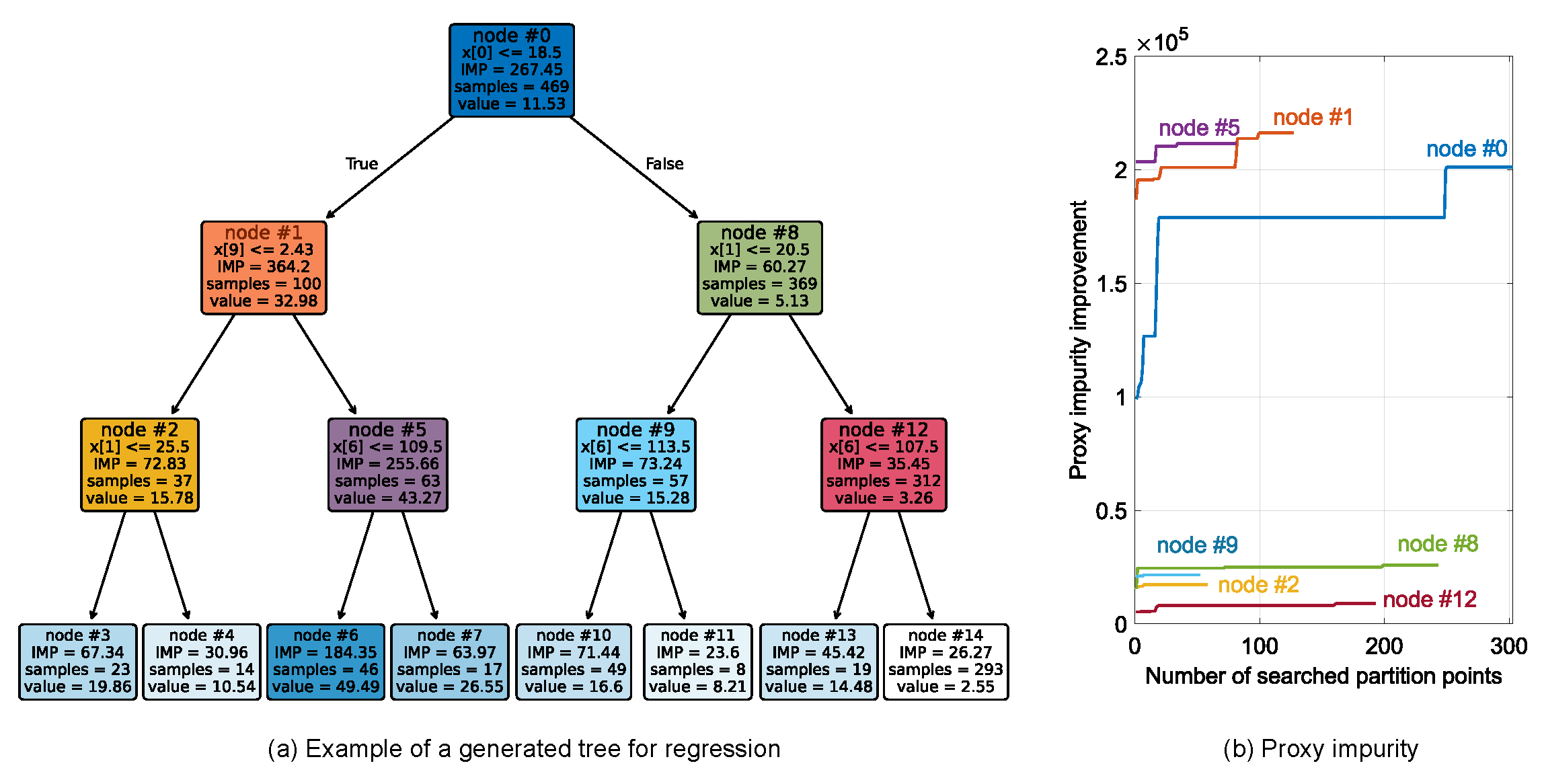
In order to exemplify the generation of both a tree and a random forest, we outline the configuration of a tree in Figure 2 and the configuration of a random forest in Figure 3. In particular, Figure 2a shows the configuration of a single tree, the feature values (denoted with x[number]), the decision thresholds, the corresponding decision branches (True to the left and False to the right), the node impurity (IMP), the number of samples in the node span, and the node value. The reader may note that, for a regression model, the value of the leaf nodes denotes the output of the tree. Also, Figure 2b denotes the values of the proxy impurity improvement when searching for the best splitting points in (6).

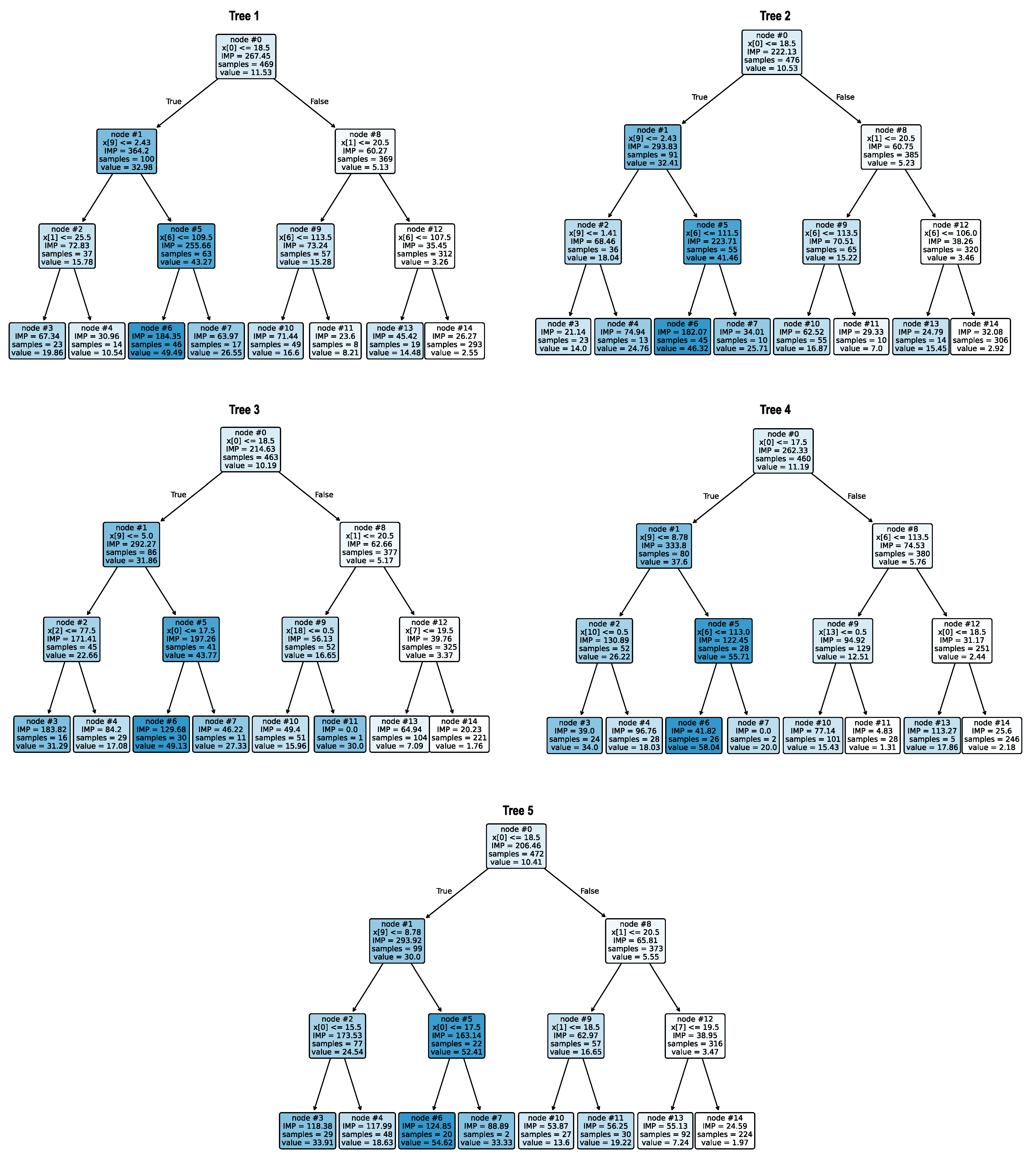
Furthermore, Figure 3 shows the configuration of all trees when we set the number of trees to five. The reader may note the relatively different configuration of each tree in terms of the decision threshold and node values. For a regression problem, the regression output is computed by the average of the five trees in Figure 3, following (16).

3.4. Data Distribution

The real-world data on the cooling conditions of steel parts comprises an imbalanced configuration, as shown with the training-testing split in Figure 4. Yet, the stratification scheme during splitting helps preserve the distribution of the classes. Furthermore, Figure 4 shows that the oversampling technique allows for an even distribution of the training data.

3.5. Regression with Default Configuration

To show a glimpse of the performance of random forest models under a default configuration scheme, Table 1 shows the results of 10 independent runs in terms of learning time and training–testing metrics. Here, metrics with the subindex n, such as in ${\mathrm{MSE}}_n$, indicate that the metric is calculated when each continuous prediction is approximated by rounding it to the nearest integer. By observing the results in Table 1, we note the following facts:

• Computation time: Random forest quickly learned the suitable fitting, in around 0.19–0.20 s per trial.
• Training Metrics: MSE ranges from 3.17 to 4.41, with high $R^2$ values above 0.98, indicating a strong model fit.
• Testing Metrics: Test MSE varies more widely (11.43 to 33.44) with $R^2$ values between 0.84 and 0.94, showing a reasonable degree of variability in generalization.
• Metrics with Nearest Approximation: MSE and $R^2$ with a nearest approximation closely follow their continuous counterparts, confirming consistency across scales.
• Overall Performance: The model demonstrates a solid training accuracy and generally good testing performance, with some trials showing a decreased test accuracy.

Table 1. Regression performance metrics (training and testing) with default configuration.

		Training				Testing
Trial	Time (s)	MSE↓	$R^{\mathbf{2}}\uparrow$	MSEn↓	$R_n^{\mathbf{2}}\uparrow$	MSE↓	$R^{\mathbf{2}}\uparrow$	MSEn↓	$R_n^{\mathbf{2}}\uparrow$
1	0.19	4.20	0.9816	4.42	0.9806	11.43	0.9351	13.00	0.9262
2	0.19	3.69	0.9829	4.59	0.9788	16.09	0.9249	17.68	0.9175
3	0.19	4.41	0.9808	4.90	0.9787	20.14	0.8813	21.36	0.8741
4	0.20	3.50	0.9836	3.95	0.9815	26.67	0.8794	27.04	0.8777
5	0.19	3.87	0.9833	4.22	0.9818	19.72	0.8804	20.10	0.8781
6	0.20	3.93	0.9833	4.44	0.9811	16.47	0.8937	16.73	0.8920
7	0.20	4.13	0.9816	4.25	0.9810	18.43	0.9038	20.63	0.8923
8	0.20	3.79	0.9825	3.74	0.9827	13.06	0.9387	13.67	0.9359
9	0.19	3.17	0.9853	3.55	0.9836	33.44	0.8429	35.92	0.8312
10	0.20	3.80	0.9812	4.19	0.9793	20.49	0.9190	22.09	0.9126

Note: Arrows describe the desirable direction of the metric for better performance: ↓ implies lower is better, ↑ implies higher is better.

Table 1. Regression performance metrics (training and testing) with default configuration.

		Training				Testing
Trial	Time (s)	MSE↓	$R^{\mathbf{2}}\uparrow$	MSEn↓	$R_n^{\mathbf{2}}\uparrow$	MSE↓	$R^{\mathbf{2}}\uparrow$	MSEn↓	$R_n^{\mathbf{2}}\uparrow$
1	0.19	4.20	0.9816	4.42	0.9806	11.43	0.9351	13.00	0.9262
2	0.19	3.69	0.9829	4.59	0.9788	16.09	0.9249	17.68	0.9175
3	0.19	4.41	0.9808	4.90	0.9787	20.14	0.8813	21.36	0.8741
4	0.20	3.50	0.9836	3.95	0.9815	26.67	0.8794	27.04	0.8777
5	0.19	3.87	0.9833	4.22	0.9818	19.72	0.8804	20.10	0.8781
6	0.20	3.93	0.9833	4.44	0.9811	16.47	0.8937	16.73	0.8920
7	0.20	4.13	0.9816	4.25	0.9810	18.43	0.9038	20.63	0.8923
8	0.20	3.79	0.9825	3.74	0.9827	13.06	0.9387	13.67	0.9359
9	0.19	3.17	0.9853	3.55	0.9836	33.44	0.8429	35.92	0.8312
10	0.20	3.80	0.9812	4.19	0.9793	20.49	0.9190	22.09	0.9126

Note: Arrows describe the desirable direction of the metric for better performance: ↓ implies lower is better, ↑ implies higher is better.

3.6. Regression with Oversampling

Also, to show a glimpse of the performance of random forest models under an oversampling scheme, Table 2 shows the results of 10 independent runs in terms of learning time and training-testing metrics. Similarly to the results described above, metrics with the subindex n indicate that these metrics were calculated when each continuous prediction was approximated by rounding it to the nearest integer. By observing the results in Table 2, we note the following facts:

• Computation Time: All trials completed rapidly, with times tightly clustered between 0.42 and 0.44 s.
• Training Metrics: Training MSE values are low (0.68 to 1.48), and $R^2$ values are consistently high (0.9961 to 0.9982), indicating an excellent model fit.
• Testing Metrics: Test MSE ranges from 11.25 to 29.19, with $R^2$ values between 0.8685 and 0.9487, reflecting strong but variable generalization.
• Metrics with Nearest Approximation: Normalized MSE and $R^2$ closely track their continuous counterparts, confirming stable performance across different scales.
• Overall Performance: Random oversampling yields robust training accuracy and generally strong testing results, with a number of trials showing a higher test error yet achieving reasonable predictive performance.

Table 2. Regression performance metrics (training and testing) with random oversampling.

		Training				Testing
Trial	Time (s)	MSE↓	$R^{\mathbf{2}}\uparrow$	MSEn↓	$R_n^{\mathbf{2}}\uparrow$	MSE↓	$R^{\mathbf{2}}\uparrow$	MSEn↓	$R_n^{\mathbf{2}}\uparrow$
1	0.42	1.10	0.9971	1.26	0.9966	11.25	0.9487	12.02	0.9452
2	0.44	0.99	0.9974	1.02	0.9973	21.46	0.9005	21.19	0.9017
3	0.42	0.78	0.9979	0.83	0.9978	21.59	0.9015	23.62	0.8922
4	0.42	0.88	0.9977	0.91	0.9976	25.79	0.8804	27.43	0.8728
5	0.42	1.03	0.9972	1.09	0.9971	18.21	0.9180	20.42	0.9080
6	0.44	1.19	0.9968	1.25	0.9967	29.19	0.8685	30.22	0.8639
7	0.44	0.86	0.9977	0.95	0.9975	18.60	0.9152	18.61	0.9151
8	0.43	0.76	0.9980	0.79	0.9979	11.66	0.9459	12.02	0.9443
9	0.44	0.68	0.9982	0.72	0.9981	13.29	0.9384	12.97	0.9399
10	0.42	1.48	0.9961	1.57	0.9958	15.51	0.9281	15.67	0.9274

Note: Arrows describe the desirable direction of the metric for better performance: ↓ implies lower is better, ↑ implies higher is better.

Table 2. Regression performance metrics (training and testing) with random oversampling.

		Training				Testing
Trial	Time (s)	MSE↓	$R^{\mathbf{2}}\uparrow$	MSEn↓	$R_n^{\mathbf{2}}\uparrow$	MSE↓	$R^{\mathbf{2}}\uparrow$	MSEn↓	$R_n^{\mathbf{2}}\uparrow$
1	0.42	1.10	0.9971	1.26	0.9966	11.25	0.9487	12.02	0.9452
2	0.44	0.99	0.9974	1.02	0.9973	21.46	0.9005	21.19	0.9017
3	0.42	0.78	0.9979	0.83	0.9978	21.59	0.9015	23.62	0.8922
4	0.42	0.88	0.9977	0.91	0.9976	25.79	0.8804	27.43	0.8728
5	0.42	1.03	0.9972	1.09	0.9971	18.21	0.9180	20.42	0.9080
6	0.44	1.19	0.9968	1.25	0.9967	29.19	0.8685	30.22	0.8639
7	0.44	0.86	0.9977	0.95	0.9975	18.60	0.9152	18.61	0.9151
8	0.43	0.76	0.9980	0.79	0.9979	11.66	0.9459	12.02	0.9443
9	0.44	0.68	0.9982	0.72	0.9981	13.29	0.9384	12.97	0.9399
10	0.42	1.48	0.9961	1.57	0.9958	15.51	0.9281	15.67	0.9274

Note: Arrows describe the desirable direction of the metric for better performance: ↓ implies lower is better, ↑ implies higher is better.

3.7. Regression with Hyperparameter Tuning

Also, to show the performance when using the hyperparameter tuning scheme, Table 3 shows the results of learning time and training–testing metrics. By observing the results in Table 3, we note the following facts:

• Computation Time: Trials completed relatively fast, with learning time ranging from 0.16 to 2.12 s and an average time of 0.87 s.
• Training Performance: The training MSE is low, at 0.99, with very high $R^2$ values averaging 0.9974.
• Testing Performance: The test MSE averages 18.46, with an $R^2$ of around 0.9173, showing a competitive predictive accuracy compared to training.
• MSE with Nearest Approximation: MSE and $R^2$ values under a nearest approximation to predictive value closely mirror their continuous counterparts, confirming stable model behavior across scales.
• Variability: Standard deviations are moderate for MSE (training: 0.28, testing: 5.52) and very low for $R^2$ coefficients (training: 0.0009, testing: 0.023), indicating consistent performance across trials.
• Computation Time: The models were learned efficiently, with learning times ranging between 0.13 and 2.05 s, averaging 1.10 s.
• Training Performance: The mean training MSE is 0.97 with very high $R^2$ values, around 0.9976, indicating a highly accurate model fit.
• Testing Performance: The test MSE averages 18.85, with an $R^2$ of approximately 0.9156, showing the strong predictive capability when unseen data are used.
• MSE with Nearest Approximation: The normalized MSE and $R^2$ under a nearest-approximation approach closely align with continuous metrics, demonstrating the stable performance across scaling.
• Variability: Moderate standard deviations for MSE (training: 0.25; testing: 5.36) and low variability for $R^2$ (training: 0.0007; testing: 0.022) reflect consistent results across trials.

Table 3. Regression performance metrics (training and testing) with hyperparameter tuning.

		Training				Testing
Trial	Time (s)	MSE↓	$R^{\mathbf{2}}\uparrow$	MSEn↓	$R_n^{\mathbf{2}}\uparrow$	MSE↓	$R^2\uparrow$	MSEn↓	$R_n^{\mathbf{2}}\uparrow$
1	2.01	1.08	0.9971	1.19	0.9968	11.13	0.9492	12.42	0.9433
2	2.12	0.99	0.9974	1.04	0.9972	22.20	0.8971	22.76	0.8945
3	0.17	0.79	0.9979	0.84	0.9978	23.91	0.8909	24.99	0.8860
4	0.17	0.88	0.9976	0.94	0.9975	22.56	0.8954	21.70	0.8994
5	0.73	1.05	0.9972	1.10	0.9971	17.70	0.9203	19.21	0.9135
6	0.18	1.15	0.9969	1.23	0.9967	26.69	0.8798	28.58	0.8713
7	1.69	0.84	0.9978	0.89	0.9976	19.01	0.9133	20.85	0.9049
8	0.21	0.73	0.9981	0.78	0.9979	11.15	0.9483	12.02	0.9442
9	0.16	0.62	0.9984	0.71	0.9981	13.93	0.9354	14.67	0.9320
10	1.25	1.47	0.9961	1.54	0.9959	15.53	0.9280	16.27	0.9246

Note: Arrows describe the desirable direction of the metric for better performance: ↓ implies lower is better, ↑ implies higher is better.

Table 3. Regression performance metrics (training and testing) with hyperparameter tuning.

		Training				Testing
Trial	Time (s)	MSE↓	$R^{\mathbf{2}}\uparrow$	MSEn↓	$R_n^{\mathbf{2}}\uparrow$	MSE↓	$R^2\uparrow$	MSEn↓	$R_n^{\mathbf{2}}\uparrow$
1	2.01	1.08	0.9971	1.19	0.9968	11.13	0.9492	12.42	0.9433
2	2.12	0.99	0.9974	1.04	0.9972	22.20	0.8971	22.76	0.8945
3	0.17	0.79	0.9979	0.84	0.9978	23.91	0.8909	24.99	0.8860
4	0.17	0.88	0.9976	0.94	0.9975	22.56	0.8954	21.70	0.8994
5	0.73	1.05	0.9972	1.10	0.9971	17.70	0.9203	19.21	0.9135
6	0.18	1.15	0.9969	1.23	0.9967	26.69	0.8798	28.58	0.8713
7	1.69	0.84	0.9978	0.89	0.9976	19.01	0.9133	20.85	0.9049
8	0.21	0.73	0.9981	0.78	0.9979	11.15	0.9483	12.02	0.9442
9	0.16	0.62	0.9984	0.71	0.9981	13.93	0.9354	14.67	0.9320
10	1.25	1.47	0.9961	1.54	0.9959	15.53	0.9280	16.27	0.9246

Note: Arrows describe the desirable direction of the metric for better performance: ↓ implies lower is better, ↑ implies higher is better.

3.8. Classification with Default Configuration

Furthermore, to show the performance of random forest classification models under a default configuration scheme, Table 4 shows the results and metrics over 10 independent runs. By observing the results in Table 4, we note the following facts:

• Computation Time: The classification models were learned at about 0.13 s. per trial, indicating a fast learning ability.
• Training Performance: The classification models fit the training data with a very low MSE (0.78–2.06) and a high $R^2$ (0.9905–0.9964), showing strong learning from training data.
• Testing Performance: The models achieved higher MSEs (27.14–63.39) and reduced $R^2$ values (0.7061–0.8778), indicating some overfitting and moderate generalization.
• Variability: The classification models achieved low variability in training metrics and moderate variability in testing metrics, implying fluctuations in model generalization across trials.

Table 4. Classification performance metrics (training and testing) with default parameters.

		Training		Testing
Trial	Time (s)	MSE↓	$R^2\uparrow$	MSE↓	$R^2\uparrow$
1	0.13	2.03	0.9905	28.21	0.8713
2	0.13	1.52	0.9929	52.10	0.7584
3	0.13	1.32	0.9938	46.65	0.7872
4	0.13	2.06	0.9905	63.39	0.7061
5	0.13	1.62	0.9924	27.14	0.8778
6	0.13	1.76	0.9918	41.94	0.8111
7	0.13	1.35	0.9937	29.60	0.8650
8	0.13	0.92	0.9957	50.37	0.7664
9	0.13	0.78	0.9964	42.50	0.8029
10	0.13	1.39	0.9936	33.67	0.8439

Note: Arrows describe the desirable direction of the metric for better performance: ↓ implies lower is better, ↑ implies higher is better.

Table 4. Classification performance metrics (training and testing) with default parameters.

		Training		Testing
Trial	Time (s)	MSE↓	$R^2\uparrow$	MSE↓	$R^2\uparrow$
1	0.13	2.03	0.9905	28.21	0.8713
2	0.13	1.52	0.9929	52.10	0.7584
3	0.13	1.32	0.9938	46.65	0.7872
4	0.13	2.06	0.9905	63.39	0.7061
5	0.13	1.62	0.9924	27.14	0.8778
6	0.13	1.76	0.9918	41.94	0.8111
7	0.13	1.35	0.9937	29.60	0.8650
8	0.13	0.92	0.9957	50.37	0.7664
9	0.13	0.78	0.9964	42.50	0.8029
10	0.13	1.39	0.9936	33.67	0.8439

Note: Arrows describe the desirable direction of the metric for better performance: ↓ implies lower is better, ↑ implies higher is better.

3.9. Classification with Oversampling

To show the performance of classification models under an oversampling scheme, Table 5 shows the rendered results in terms of learning and performance metrics. By observing Table 5, we note the following facts:

• Computation Time: Slightly increased compared to default parameters, ranging from 0.20 to 0.21 s. per trial, yet remains consistent and efficient.
• Training Performance: Models achieved low MSEs (0.73–1.96) and high $R^2$ values (0.9948–0.9980), indicating an excellent fit with the training data.
• Testing Performance: The models achieved an improved MSE in some trials compared to the ones with default parameters, with MSEs ranging from 28.57 to 59.56 and $R^2$ values ranging from 0.7238 to 0.8697, showing the moderate generalization and the reduction in overfitting.
• Variability: The models achieved low variability in computation times and training metrics and moderate variability in testing metrics, reflecting fluctuations in model generalization across trials.

Table 5. Classification performance metrics (training and testing) with random oversampling.

		Training		Testing
Trial	Time (s)	MSE↓	$R^2\uparrow$	MSE↓	$R^2\uparrow$
1	0.21	1.42	0.9962	28.57	0.8697
2	0.21	1.19	0.9968	45.69	0.7881
3	0.20	0.93	0.9975	47.56	0.7830
4	0.21	1.42	0.9962	59.56	0.7238
5	0.21	1.42	0.9962	33.58	0.8487
6	0.20	1.62	0.9957	44.76	0.7984
7	0.20	1.14	0.9970	31.84	0.8547
8	0.20	0.73	0.9980	52.08	0.7585
9	0.21	0.78	0.9979	34.08	0.8420
10	0.20	1.96	0.9948	34.17	0.8415

Note: Arrows describe the desirable direction of the metric for better performance: ↓ implies lower is better, ↑ implies higher is better.

Table 5. Classification performance metrics (training and testing) with random oversampling.

		Training		Testing
Trial	Time (s)	MSE↓	$R^2\uparrow$	MSE↓	$R^2\uparrow$
1	0.21	1.42	0.9962	28.57	0.8697
2	0.21	1.19	0.9968	45.69	0.7881
3	0.20	0.93	0.9975	47.56	0.7830
4	0.21	1.42	0.9962	59.56	0.7238
5	0.21	1.42	0.9962	33.58	0.8487
6	0.20	1.62	0.9957	44.76	0.7984
7	0.20	1.14	0.9970	31.84	0.8547
8	0.20	0.73	0.9980	52.08	0.7585
9	0.21	0.78	0.9979	34.08	0.8420
10	0.20	1.96	0.9948	34.17	0.8415

Note: Arrows describe the desirable direction of the metric for better performance: ↓ implies lower is better, ↑ implies higher is better.

3.10. Classification with Hyperparameter Tuning

Finally, to show the performance of classification models with the hyperparameter tuning scheme, Table 6 shows the rendered performance metrics. By observing Table 6, we note the following facts:

• Computation Time: The models were learned with more variability compared to previous approaches, with learning times ranging from 0.09 to 1.80 s. per trial, reflecting the increased computational cost of 10-fold cross-validation.
• Training Performance: The models achieved low MSEs (0.73–1.96) and high $R^2$ values (0.9948–0.9980), indicating a strong model fit on training data.
• Testing Performance: The model achieved MSEs on testing ranging from 15.65 to 54.46 and $R^2$ values from 0.7516 to 0.9274, suggesting better generalization and reduced overfitting in certain cases.
• Variability: The models achieved high variability in computation times and moderate variability in testing metrics, reflecting the effects of cross-validation and parameter tuning on model performance.

Table 6. Classification performance metrics using hyperparameter tuning.

		Training		Testing
Trial	Time (s)	MSE↓	$R^2\uparrow$	MSE↓	$R^2\uparrow$
1	1.66	1.42	0.9962	17.99	0.9179
2	0.23	1.19	0.9968	43.62	0.7977
3	0.09	0.93	0.9975	54.46	0.7516
4	0.41	1.42	0.9962	43.15	0.7999
5	0.16	1.42	0.9962	23.39	0.8947
6	0.17	1.62	0.9957	36.82	0.8342
7	1.08	1.14	0.9970	28.72	0.8690
8	0.11	0.73	0.9980	33.35	0.8454
9	1.58	0.78	0.9979	15.65	0.9274
10	1.80	1.96	0.9948	21.84	0.8987

Note: Arrows describe the desirable direction of the metric for better performance: ↓ implies lower is better, ↑ implies higher is better.

Table 6. Classification performance metrics using hyperparameter tuning.

		Training		Testing
Trial	Time (s)	MSE↓	$R^2\uparrow$	MSE↓	$R^2\uparrow$
1	1.66	1.42	0.9962	17.99	0.9179
2	0.23	1.19	0.9968	43.62	0.7977
3	0.09	0.93	0.9975	54.46	0.7516
4	0.41	1.42	0.9962	43.15	0.7999
5	0.16	1.42	0.9962	23.39	0.8947
6	0.17	1.62	0.9957	36.82	0.8342
7	1.08	1.14	0.9970	28.72	0.8690
8	0.11	0.73	0.9980	33.35	0.8454
9	1.58	0.78	0.9979	15.65	0.9274
10	1.80	1.96	0.9948	21.84	0.8987

Note: Arrows describe the desirable direction of the metric for better performance: ↓ implies lower is better, ↑ implies higher is better.

3.11. Overall Comparison

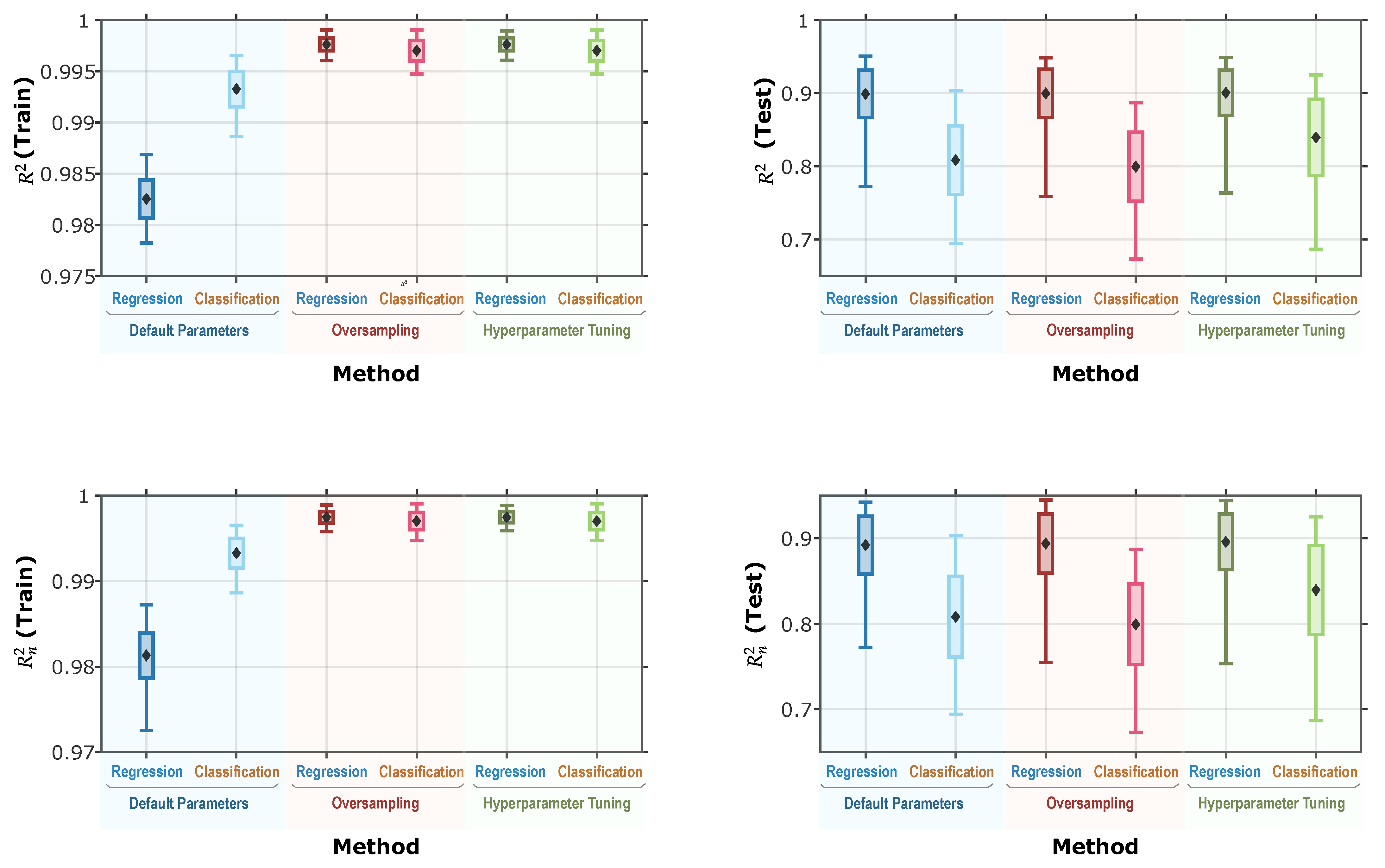
In order to compare the performance of the above-mentioned random forest models, we performed 100 independent runs and compared the MSE and $R^2$ metrics, as shown in Figure 5 and Figure 6, respectively. By looking at these results, one can note the following facts:

• Random forests utilizing oversampling and hyperparameter tuning outperform the default configuration in both MSE and $R^2$ metrics. However, the difference in performance between oversampling and hyperparameter tuning alone is not substantial. Given that hyperparameter tuning is a relatively computationally intensive process, the oversampling approach provides comparable performance benefits with significantly lower computational costs, making it a more efficient choice in practice.
• Although classification models initially outperformed regression models under default parameter configurations, the performance gap between the two approaches diminished significantly when oversampling and hyperparameter tuning were applied. In fact, regression models consistently outperformed classification models across all instances on the testing dataset. This finding underscores the practical advantages of using regression trees for estimating the cooling conditions of steel parts.

Figure 5. Comparison of MSE over 100 independent runs (smaller MSE values are better).

Figure 5. Comparison of MSE over 100 independent runs (smaller MSE values are better).

Figure 6. Comparison of $R^2$ coefficient over 100 independent runs (higher values of $R^2$ are better).

Figure 6. Comparison of $R^2$ coefficient over 100 independent runs (higher values of $R^2$ are better).

3.12. Feature Importance

To illustrate the importance of each feature in constructing decision trees within a random forest, Figure 7 presents the degree of importance for nine independent random forest models derived from a regression under an oversampling scheme. By examining the results in Figure 7, we observed the following key findings:

• Chemical Composition: Carbon and chromium were found to play significant roles in determining the cooling conditions of steel parts. In heat treatment, carbon is widely recognized as the most influential element, as it directly affects wear resistance, hardness, and strength. The microstructural properties of metals are influenced by both cooling rates and chemical composition [16,17,18,19]. Under air cooling, increasing the carbon content induces an increase in hardness and brittleness [32]. Our results showed that carbon was the most important feature when decision trees were constructed to predict the cooling parameters of steel parts. Furthermore, chromium, which is also considered important in heat treatment due to its effect on hardenability and corrosion resistance, exhibited relatively high importance values in our analysis.
• Material: No consistent pattern was observed regarding the importance of the seven materials in model development. While some materials contributed more than others, there were no notable commonalities among them. Overall, this suggests that material type is not a significant factor in determining the cooling conditions of steel parts.
• Weight: After carbon, the weight of each steel part emerged as the second most important factor in building decision trees for estimating cooling parameters. This can be attributed to the well-known mass effect in steel-part annealing: heavier parts are less likely to be quenched thoroughly to the center, whereas smaller parts cool more quickly and uniformly, making complete quenching easier. Thus, differences in mass directly influence the efficiency of heat transfer and cooling, establishing weight as a crucial factor in determining optimal cooling conditions.
• Shape: Although it was initially thought that the ease of heat conduction due to part shape might have a significant impact, overall, none of the shapes emerged as particularly important factors. However, the washer and ring shapes showed relatively higher importance. This is likely because both shapes have a hollow center, which facilitates more efficient cooling compared to other shapes.

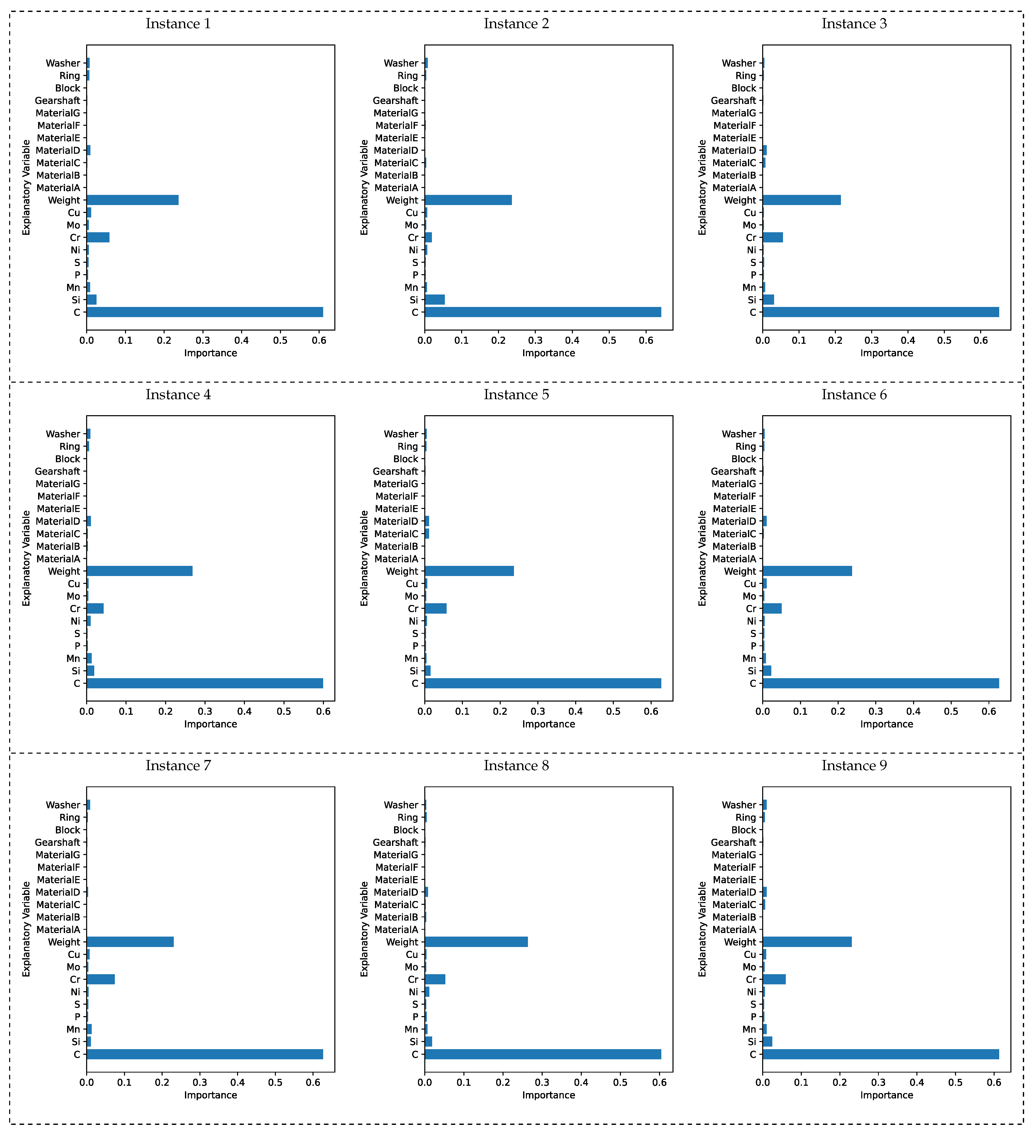
Based on the above findings, the amounts of chemical components—particularly carbon and chromium—as well as the weight of the steel parts, were identified as key factors in constructing highly effective decision trees for determining optimal cooling conditions. Using only these explanatory variables, it is possible to build decision trees that achieve a coefficient of determination $R^2$ of 0.92, indicating performance nearly equivalent to regression models that include all explanatory variables. Conversely, since other factors contribute only marginally to model improvement, focusing on chemical composition and weight is both efficient and practical for real-world applications. The above observations align closely with the practical expertise of seasoned operators who routinely recommend cooling parameters for the metal-annealing process.

Our results highlight that both the intrinsic properties of steel parts (determined mainly by C and Cr composition) and extrinsic factors such as part weight collectively govern the cooling parameter and, thus, the resulting microstructure. From a heat-transfer perspective, the chemical composition in terms of C and Cr influences several key thermal properties: (1) Regarding surface oxide characteristics, chromium (Cr) is known to form stable and protective oxide layers [33]. These layers act as thermal barriers and reduce the rate of heat transfer from the steel to the environment. In contrast, steels with higher carbon (C) but low chromium (Cr) tend to form less-protective iron oxides, which are less effective at impeding the heat flow; thus, the composition of both C and Cr influences surface heat transfer during cooling. (2) Regarding the heat-transfer coefficient within steel, a higher C content in steel reduces thermal conductivity due to C atoms acting as scattering centers for heat carriers (electrons and phonons), thus making it difficult for heat to move from the steel’s interior to its surface. Similarly, the addition of Cr changes steel’s microstructure and lattice, introducing further scattering sites, which lowers thermal conductivity compared to plain carbon steels. As a result, steels with higher C and Cr content exhibit more distorted crystal structures and increased electron scattering, impeding the conduction of heat and causing them to cool more slowly. (3) Regarding the latent heat of phase transformation, the latent heat released or absorbed during steel phase transformations is strongly influenced by C and Cr. While carbon can shift the transformation temperatures of steel, chromium can stabilize certain phases and alter the transformation pathway. These changes in the transformation pathway affect the amount of energy that must be removed for the steel to fully transform, thus potentially impacting the cooling rate. (4) Regarding specific heat, carbon enables the formation of iron carbide, which changes the microstructure and thereby influences how thermal energy is absorbed and stored in steel. Chromium primarily influences steel’s hardenability, thereby potentially lowering the critical cooling rate required to form martensite during quenching. (5) Regarding the surface heat-transfer coefficient, chromium (Cr) enhances the formation of a dense, protective oxide layer, potentially reducing the thermal conductivity and decreasing the rate at which heat can be transferred to the cooling medium.

Additionally, to validate our observations, we processed approximately 40 steel parts in a real-world setting using parameter values estimated from one of the constructed decision trees. The applied parameters consistently resulted in the hardenability of the steel parts falling within the standard acceptable range. These results show the practical feasibility of using random forests for predicting the cooling conditions in steel part annealing.

Further accuracy improvements are expected as data continues to be accumulated. While the random forest inherently includes stochastic elements, prediction performance can be maintained by increasing the number of trees and the tree depth and by using ensemble averaging. Additionally, since training time occurs on the order of less than one second (about 0.4 s when random oversampling is used), carefully selected additional data has the potential to improve model generalization for existing models by covering a wider range of cooling conditions.

Although our study has focused on air-based cooling rate parameters, further research to elucidate the feasibility of random forests in modeling other commonly used heat treatment processes with high repeatability—such as vacuum heat treatment (HT) combined with gas cooling—remains highly relevant for industry. These processes are valued for their controlled cooling rates, which help achieve consistent microstructures and mechanical properties. Given the diversity of cooling media—including water, oil, polymers, and gases—each with distinct effects on steel microstructure, developing reliable cooling rate prediction models for such standard processes has the potential to enhance predictability and quality control. This targeted approach could also streamline industrial process optimization and reduce trial and error in production environments.

Our results demonstrate the feasibility of using random forests to predict cooling rates in steel part annealing. However, as steels exhibit diverse transformation behaviors, depending on their composition and cooling conditions—as illustrated by the variety of continuous cooling transformation (CCT) diagrams available for different grades—an enhanced dataset that includes a broader range of steels, along with validation against experimental cooling diagrams, has the potential to aid in constructing robust random forest models applicable across different steel grades and heat treatment scenarios.

Figure 7. Feature importance over nine independent instances using regression under an oversampling scheme.

Figure 7. Feature importance over nine independent instances using regression under an oversampling scheme.

Furthermore, although we considered the geometry of steel parts as one feature, size and batch limits may play important roles in cooling rate prediction. For instance, oversized steel parts and larger batch sizes may lead to non-uniform temperature distribution and cooling rates, potentially impacting microstructure composition. In future work, we plan to investigate the effect of steel part size and batch limits on cooling-rate prediction within heat treatment contexts, further elucidating the reliability of random forests within practical boundaries.

4. Conclusions

We investigated the feasibility of using random forests to predict cooling-rate parameters for the heat treatment of steel parts. Our computational experiments, based on real-world records collected from the daily operations of an industrial furnace and cooling device operator, demonstrated the advantageous properties of regression random forest models, particularly when combined with an oversampling scheme. We also found that the chemical composition—specifically, the carbon and chromium content—as well as the weight of the steel parts, are key factors in constructing highly effective decision trees for estimating optimal cooling conditions. These findings highlight the effectiveness and practical value of random forests for estimating cooling conditions in steel part annealing. The ensemble approach of random forests, along with their ability to handle feature interactions, makes them well-suited to modeling useful decision trees, further emphasizing their practical applicability for industrial annealing processes.

References

1. Yi, Q.; Wu, X.; Zhuo, J.; Li, C.; Li, C.; Cao, H. An incremental data-driven approach for carbon emission prediction and optimization of heat treatment processes. Case Stud. Therm. Eng. 2025, 72, 106320. [Google Scholar] [CrossRef]
2. Mudda, S.; Hegde, A.; Sharma, S.; Gurumurthy, B. Optimization of various heat treatment parameters for superior combination of hardness and impact energy of AISI 1040 steel. J. Mater. Res. Technol. 2025, 38, 3900–3908. [Google Scholar] [CrossRef]
3. Yang, P.; Su, H.; Guo, Y.; Zhou, H.; Xia, L.; Shen, Z.; Wang, M.; Zhang, Z.; Guo, M. Influence of cooling rate during the heat treatment process on the precipitates and ductility behavior of inconel 718 superalloy fabricated by selective laser melting. Mater. Sci. Eng. A 2024, 902, 146603. [Google Scholar] [CrossRef]
4. Yan, M.; Zhang, H.; Yang, F.; Gui, Y.; Han, Z.; Fu, H. The Effect of Heat Treatment on the Microstructure and Mechanical Properties of Powder Metallurgy Ti-48Al Alloy. Metals 2024, 14, 661. [Google Scholar] [CrossRef]
5. Lütjering, G. Influence of processing on microstructure and mechanical properties of (α + β) titanium alloys. Mater. Sci. Eng. A 1998, 243, 32–45. [Google Scholar] [CrossRef]
6. Zhang, K.; Hu, R.; Li, J.; Yang, J.; Gao, Z. Grain refinement of 1 at.% Ta-containing cast TiAl-based alloy by cyclic air-cooling heat treatment. Mater. Lett. 2020, 274, 127940. [Google Scholar] [CrossRef]
7. Yao, X.; Wang, W.; Qi, X.; Lv, Y.; Yang, W.; Li, T.; Chen, J. Effects of heat treatment cooling methods on precipitated phase and mechanical properties of CoCrFeMnNi–Mo5C0.5 high entropy alloy. J. Mater. Res. Technol. 2024, 29, 3566–3574. [Google Scholar] [CrossRef]
8. Milenkovic, S.; Sabirov, I.; LLorca, J. Effect of the cooling rate on microstructure and hardness of MAR-M247 Ni-based superalloy. Mater. Lett. 2012, 73, 216–219. [Google Scholar] [CrossRef]
9. Patil, M.A.; Ghara, T.; Das, B.; Kulkarni, D.M. Influence of cooling rate on microstructure, dislocation density, and associated hardness of laser direct energy deposited Inconel 718. Surf. Coat. Technol. 2025, 495, 131575. [Google Scholar] [CrossRef]
10. Hall, E.O. The Deformation and Ageing of Mild Steel: III Discussion of Results. Proc. Phys. Soc. Sect. B 1951, 64, 747. [Google Scholar] [CrossRef]
11. Petch, N.J. The Cleavage Strength of Polycrystals. J. Iron Steel Inst. 1953, 174, 25–28. [Google Scholar]
12. Shin, B.H.; Park, J.; Jeon, J.; Heo, S.B.; Chung, W. Effect of cooling rate after heat treatment on pitting corrosion of super duplex stainless steel UNS S 32750. Anti-Corros. Methods Mater. 2018, 65, 492–498. [Google Scholar] [CrossRef]
13. Skulkina, N.; Ivanov, O.; Deanisov, N.; Chekis, V. Cooling rate upon in air heat treatment and magnetic properties of amorphous soft magnetic alloys. J. Magn. Magn. Mater. 2019, 470, 156–158. [Google Scholar] [CrossRef]
14. Ahmed, M.; Savvakin, D.G.; Ivasishin, O.M.; Pereloma, E.V. The effect of cooling rates on the microstructure and mechanical properties of thermo-mechanically processed Ti–Al–Mo–V–Cr–Fe alloys. Mater. Sci. Eng. A 2013, 576, 167–177. [Google Scholar] [CrossRef]
15. Xu, J.; Zeng, W.; Zhao, Y.; Sun, X.; Du, Z. Influence of cooling rate following heat treatment on microstructure and phase transformation for a two-phase alloy. J. Alloys Compd. 2016, 688, 301–309. [Google Scholar] [CrossRef]
16. Feng, L.; Hu, F.; Zhou, W.; Ke, R.; Zhang, G.; Wu, K.; Qiao, W. Influences of Alloying Elements on Continuous Cooling Phase Transformation and Microstructures of Extremely Fine Pearlite. Metals 2019, 9, 70. [Google Scholar] [CrossRef]
17. Dey, I.; Ghosh, S.K.; Saha, R. Effects of cooling rate and strain rate on phase transformation, microstructure and mechanical behaviour of thermomechanically processed pearlitic steel. J. Mater. Res. Technol. 2019, 8, 2685–2698. [Google Scholar] [CrossRef]
18. Gao, M.; Yang, J.; Zhang, Y.; Song, H. Effect of Alloying Elements on Pearlite Critical Cooling Rate of U75V Rail-steel. Trans. Indian Inst. Met. 2023, 76, 665–673. [Google Scholar] [CrossRef]
19. Abdali, A.; Hossein Nedjad, S.; Hamed Zargari, H.; Saboori, A.; Yildiz, M. Predictive tools for the cooling rate-dependent microstructure evolution of AISI 316L stainless steel in additive manufacturing. J. Mater. Res. Technol. 2024, 29, 5530–5538. [Google Scholar] [CrossRef]
20. Li, Q.; Wang, J.; Xue, C.; Miao, Y.; Hou, Q.; Meng, Y.; Yang, X.; Li, X. Quantifying the effects of cooling rates on Fe-rich intermetallics in recycled Al-Si-Cu alloys by machine learning. J. Alloys Compd. 2025, 1014, 178718. [Google Scholar] [CrossRef]
21. Geng, X.; Mao, X.; Wu, H.H.; Wang, S.; Xue, W.; Zhang, G.; Ullah, A.; Wang, H. A hybrid machine learning model for predicting continuous cooling transformation diagrams in welding heat-affected zone of low alloy steels. J. Mater. Sci. Technol. 2022, 107, 207–215. [Google Scholar] [CrossRef]
22. Afflerbach, B.T.; Francis, C.; Schultz, L.E.; Spethson, J.; Meschke, V.; Strand, E.; Ward, L.; Perepezko, J.H.; Thoma, D.; Voyles, P.M.; et al. Machine Learning Prediction of the Critical Cooling Rate for Metallic Glasses from Expanded Datasets and Elemental Features. Chem. Mater. 2022, 34, 2945–2954. [Google Scholar] [CrossRef]
23. Schultz, L.E.; Afflerbach, B.; Voyles, P.M.; Morgan, D. Machine learning metallic glass critical cooling rates through elemental and molecular simulation based featurization. J. Mater. 2025, 11, 100964. [Google Scholar] [CrossRef]
24. Akif Koç, M.; Ahlatci, H.; Esen, İ.; Eroğlu, M. Prediction of accelerated cooling rates in H-section steels using artificial neural networks. Case Stud. Therm. Eng. 2025, 74, 106939. [Google Scholar] [CrossRef]
25. Liu, A.; Liu, F.; Zhao, S.; Ren, R.; Zhou, Y.; Shi, T.; Liu, J. Prediction of critical cooling rate under rapid heating rate and short holding time for pearlitic rail steel. J. Mater. Res. Technol. 2025, 36, 6534–6541. [Google Scholar] [CrossRef]
26. Pedregosa, F.; Varoquaux, G.; Gramfort, A.; Michel, V.; Thirion, B.; Grisel, O.; Blondel, M.; Prettenhofer, P.; Weiss, R.; Dubourg, V.; et al. Scikit-learn: Machine Learning in Python. J. Mach. Learn. Res. 2011, 12, 2825–2830. [Google Scholar]
27. Scikit-Learn: Machine Learning in Python, Version 1.7.2. 2025. Available online: https://scikit-learn.org/stable/ (accessed on 7 September 2025).
28. Breiman, L. Random Forests. Mach. Learn. 2001, 45, 5–32. [Google Scholar] [CrossRef]
29. Breiman, L. Bagging predictors. Mach. Learn. 1996, 24, 123–140. [Google Scholar] [CrossRef]
30. Breiman, L.; Friedman, J.; Olshen, R.A.; Stone, C.J. Classification and Regression Trees, 1st ed.; Chapman and Hall/CRC: New York, NY, USA, 1984. [Google Scholar] [CrossRef]
31. Sequential Model-Based Optimization in Python, Version 0.8.1. 2025. Available online: https://scikit-optimize.github.io/stable/index.html (accessed on 7 September 2025).
32. Wang, X.; Chen, Y.; Wei, S.; Zuo, L.; Mao, F. Effect of Carbon Content on Abrasive Impact Wear Behavior of Cr-Si-Mn Low Alloy Wear Resistant Cast Steels. Front. Mater. 2019, 6, 153. [Google Scholar] [CrossRef]
33. Hebbale, A.M.; Ramesh, M.; Petru, J.; Chandramouli, T.; Srinath, M.; Shetty, R.K. A microstructural study and high-temperature oxidation behaviour of plasma sprayed NiCrAlY based composite coatings. Results Eng. 2025, 25, 103926. [Google Scholar] [CrossRef]
Figure 1. Concept of fan-assisted air cooling in the heat treatment of steel parts.
Applsci 15 11676 g001
Figure 2. (a) Example of a tree and (b) impurity improvement when searching for node splits. Each non-terminal node generates left and right children, following a splitting strategy that aims to maximize the proxy impurity improvement metric.
Applsci 15 11676 g002
Figure 3. Example of trees in a random forest model for regression and the associated thresholds, impurity, and values in each node.
Applsci 15 11676 g003
Figure 4. Data distribution in training (left), testing (center), and oversampling mechanism (right).
Applsci 15 11676 g004
Disclaimer/Publisher’s Note: The statements, opinions and data contained in all publications are solely those of the individual author(s) and contributor(s) and not of MDPI and/or the editor(s). MDPI and/or the editor(s) disclaim responsibility for any injury to people or property resulting from any ideas, methods, instructions or products referred to in the content.