Abstract
This study investigates the optimization of crushing and screening efficiency in hammer mill systems through aerodynamic analysis. The research focuses on cucumber vine stalks characterized by high moisture content, elevated cellulose concentration, and pronounced mechanical toughness. Using key operating parameters that significantly influence the gas flow field as the starting point, single-phase gas flow field numerical simulations and characteristic simulations were conducted using the computational fluid dynamics (CFD) software Fluent. A two-way coupling method combining Fluent and the discrete element method (DEM) software EDEM was employed to perform gas–solid coupled numerical simulations and operational characteristic simulations of the pulverizer’s grinding and screening process. This revealed the influence patterns of gas flow disturbances on the grinding and screening process and the mechanism for performance enhancement. Finally, field testing was conducted. Based on experimental results, the optimized operating parameters were determined as follows: rotor speed of 2569 r/min, fan opening of 62.55%, and feed rate of 7.64 kg/min. Under these optimized conditions, the crushing productivity of cucumber vine stalks reached 337 kg/h, with an energy consumption of 5.59 kW·h/t. The deviation between the actual and theoretical values for productivity was less than 6%, while the deviation for energy consumption per ton was less than 3%. These findings provide a theoretical foundation and experimental basis for further research into the mechanism of external airflow disturbance in the crushing and screening process, aiming to enhance crushing efficiency and reduce energy consumption.
1. Introduction
Comminution of crop residues constitutes a critical stage in agricultural waste processing. Cucumber stalks, characterized by elevated moisture content, axial entanglement tendencies, and low bulk density, present significant challenges in mechanical comminution [1,2,3]. The hammer mill remains the predominant technology for lignocellulosic biomass size reduction [4,5,6]. During operation, these machines generate complex aerodynamic fields within their crushing chambers, which critically influence particle comminution kinetics and screening efficiency. Consequently, systematic investigation of airflow dynamics within the hammer mill holds substantial importance for optimizing biomass processing performance. Current research on hammer mill aerodynamics predominantly focuses on elucidating structural influences on intra-chamber airflow patterns.
The current research on the airflow field in the pulverizing chamber of hammer mill mainly focuses on the effect of the pulverizing structure on the airflow field in the pulverizing chamber. Li-Ying Cao et al. [7] pioneered a virtual instrumentation-based flow field measurement system for hammer mills, where BP neural networks coupled with genetic algorithms interpolated spatial pressure distributions from 49 discrete measurement points, ultimately generating high-resolution pressure cloud visualizations of the comminution chamber aerodynamics; Qian et al. [8] employed ANSYS Fluent to computationally analyze turbulent flow dynamics induced by three geometrically distinct screen configurations (arc-segmented, helical, and radial patterns) in biomass pulverizers. The study demonstrated that interrupted-segmented-arc screens generated controlled vorticity zones within the annular recirculation region, effectively increasing material throughput efficiency compared to conventional designs; Budăcan et al. [9] conducted CFD-based computational analyses to characterize multiphase flow dynamics within industrial hammer mill chambers. Their investigation identified persistent turbulence phenomena in the annular recirculation layer, with the resultant fluid–particle interactions exerting deterministic control over particulate morphology evolution and energy transfer mechanisms during comminution processes; Zhang et al. [10] employed CFD simulations (ANSYS Fluent) to investigate the aerodynamic effects of rotor geometry and screen aperture ratios on the 9FF-series corn stover crusher. Their findings demonstrated that optimized rotor-screen geometric configurations significantly enhanced material transport efficiency by modulating turbulent kinetic energy dissipation patterns within the comminution chamber. Current research exhibits a critical gap in understanding the flow field perturbations induced by external aerodynamic interactions. While optimized airflow characteristics demonstrably enhance mill throughput and mitigate sieve-clogging risks, the fundamental mechanisms governing rotor-fan-system-induced turbulent flow regimes remain poorly characterized.
In practical applications, particle motion often occurs within complex flow fields. Gas–solid coupling methods [11,12,13], which fully account for the interactions between the airflow and particle assemblies, provide more realistic simulations.
The application of gas–solid coupling in crusher research remains limited, with most studies employing the Dense Phase Model (DPM) in Fluent [14,15]. Takeuchi [16,17] used a CFD-DPM approach to analyze the flow field and particle motion within an impact crusher, concluding that high-speed rotor rotation creates a circulating airflow layer. This, combined with direct rotor contact, accelerates particles beyond the rotor tip speed. Using Hertzian theory, they correlated impact stress with impact velocity.
Studies using the coupled CFD-DEM method for crushers are even scarcer. In 2021, Bhonsale [18] utilized CFD-DEM to analyze the relationship between particle and airflow velocities inside a crusher, demonstrating that the airflow is also influenced by the particles. In 2023, Feng Yutao [19] investigated the back-feeding process of particles driven by airflow in a crusher with a recirculation device using CFD-DEM. The results showed that a modified screen design increased the passing rate by 32.65% compared to the original. However, these studies did not simulate the actual breakage process of particles.
In summary, while gas–solid coupling methods are widely used in agricultural machinery to optimize design and operational parameters by evaluating their impact on performance, Fluent’s multiphase models often treat the material only as a continuum, lacking a quantitative description of individual non-spherical particle motion. In contrast, this paper establishes a coupled CFD-DEM model that simultaneously simulates the airflow, particle interactions, and the breakage process itself, resulting in a more comprehensive and realistic numerical simulation that better aligns with actual production conditions.
2. Theoretical Analysis
2.1. Mathematical Model
Assuming the density of the gas within the pulverizer remains constant, the gas can be regarded as an incompressible fluid. This is in accordance with the fundamental principles of mass, momentum, and energy conservation. For incompressible fluids, energy conservation does not consider thermodynamic energy conversion. This can be derived by integrating the conservation of mass with the conservation of momentum.
Bidirectional coupling generates interactions between the particle phase and the fluid phase. Coupling control equations are established between the two phases by introducing an interphase momentum term. These equations can be categorized into fluid-phase control equations and particle-phase control equations, which, respectively, describe the coupled behavior between the two phases.
- (1)
- Mass Conservation Governing Equation
The principle of mass conservation in fluid dynamics dictates that the temporal rate of mass accumulation within a differential fluid element must equal the net mass flux across its boundaries. This fundamental law, mathematically formalized as the continuity equation, governs fluid motion through the following expressions:
, where is a constant; the governing mass conservation equation for the multiphase flow within the pulverization chamber can be reduced to the following simplified form:
where is fluid density, is the flow time, , uy, uz are the components of the fluid velocity in the direction of , and .
- (2)
- Momentum Conservation Control Equation
The momentum conservation principle in fluid systems establishes that the temporal variation in momentum of a discrete fluid element precisely corresponds to the resultant of surface forces acting on its boundaries and body forces distributed throughout its volume. The momentum conservation control equation can be expressed as follows:
where is hydrostatic pressure acting on the fluid element, is viscous stress tensor components (i = n: normal direction, j = t: tangential direction), , Fy, and are cartesian components of body force per unit mass.
- (3)
- The interaction between straw particles and the gas flow generates a momentum source, which can be expressed as follows:
Further analysis of the particle-phase control equations reveals that the motion of straw particles within the crushing chamber primarily consists of translational and rotational components. According to Newton’s second law, these motions can be described as follows:
where is the mass of the straw particle, kg; is the velocity of the straw particle, m/s; is the contact force acting on the straw particle, N; is the force exerted by the airflow on the straw particle, N; is the rotational inertia of the straw particle, kg·m2; is the angular velocity of the straw particle, rad/s; is the torque generated by the contact force, N·m; is the torque generated by the airflow acting on the straw particle, N·m.
The forces exerted by airflow on straw particles manifest as drag force, pressure gradient force, and Magnus force, among others [20,21,22]. Among these, drag force represents the primary force exerted by airflow on straw particles. This study adopts the widely applicable free-stream drag model. The free-stream drag model expression is as follows:
where is the drag coefficient; is the particle diameter, m; is the air density, taken as 1.29 kg/m3.
The contact force model selected for straw particles is the Hertz–Mindlin with bonding model. The crushing process involves the gradual reduction in straw particle size, and the Hertz–Mindlin with bonding model is derived from the Hertz–Mindlin (no slip) contact model [23]. Building upon the calculation of fundamental contact forces between particles, it establishes parallel bonding between adjacent particle contact points, forming adhesive bonds that generate forces and moments between particles, as shown in Figure 1. When these adhesive bonds are disrupted by external forces, they do not reconnect. The simulation of fragmentation and fracture phenomena is achieved through the breaking of these adhesive bonds. The forces and moments acting on the adhesive bonds are as follows:
where , are the tangential and normal cohesive force, N; , are the tangential and normal cohesive stress moment, N·m; are the particle tangential and normal velocity, m/s; are the unit area tangential and normal stiffness, N/m; is the cohesive bond cross-sectional area, m2; is the moment of inertia, kg·m2; is the time step, s; is the bond radius, m.
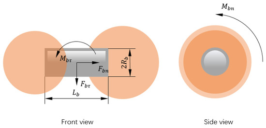
Figure 1.
Bonding adhesion model.
When the external force acting on the adhesive bond exceeds the critical stress in the tangential and normal directions, the adhesive bond will fracture, which can be expressed as follows:
Among these, and represent the critical stress in the tangential and normal directions, Pa.
2.2. Geometric Model of the Hammer Mill
The self-developed comminution apparatus incorporates a dual-tangential air intake configuration at the upper periphery of the pulverization chamber. This counter-rotating airflow design aims to optimize the vortex flow characteristics through shear layer interaction. Geometric simplification was implemented following aerodynamic equivalence analysis, preserving critical flow-governing features while eliminating non-essential structural components to facilitate CFD meshing processes and reduce simulation complexity. The physical prototype configuration (Figure 2a) and its aerodynamically equivalent simplified counterpart (Figure 2b). Crusher component parameters are listed in Table 1.
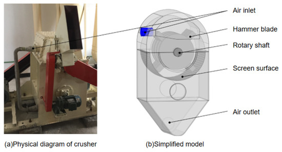
Figure 2.
Physical diagram and simplified model of a crusher.

Table 1.
Crusher component parameters.
2.3. Turbulence Model
Fluid flow regimes can be classified into three distinct categories: laminar, transitional, and turbulent flows, characterized by their respective Reynolds number ranges, velocity profile structures, and energy dissipation mechanisms. The pulverization chamber exhibits a highly transient multiphase flow field dominated by biomass particle–airflow coupling transport phenomena. Non-orthogonal flow channel geometry with heterogeneous boundary conditions induces non-stationary vortex dissipation patterns. Critical Reynolds number analysis (Re > 2000) confirms the fully developed turbulent flow regime, thereby justifying the application of the Reynolds-averaged Navier–Stokes (RANS) turbulence modeling for numerical simulation.
The Reynolds-averaged Navier–Stokes (RANS) methodology employs time-filtering operations to decompose instantaneous flow variables into mean and fluctuating components, establishing the Reynolds stress tensor closure problem. The standard turbulence model, derived from the Boussinesq eddy-viscosity hypothesis with isotropic turbulence dissipation assumptions is selected due to its demonstrated computational robustness in industrial applications involving complex flow separations and recirculation zones.
The standard model constitutes a two-equation eddy-viscosity closure, where the turbulent kinetic energy (k) and its dissipation rate () are governed by coupled transport equations. For incompressible flows, the system is expressed as follows:
where is the turbulent Prandtl number for turbulent kinetic energy k; is the turbulent Prandtl number for turbulent dissipation rate ; and are the flow length and velocity in the direction; is the production of turbulent kinetic energy due to mean velocity gradients. Following the standard calibration by Launder and Spalding, the values of these constants are adopted as follows: , .
2.4. Fluid Domain Model
The computational analysis of flow fields necessitates the development of a fluid domain model, which precisely represents the internal airflow dynamics within the comminution chamber of the grinding system. The upper region of the geometric model was designated as the fluid domain, as illustrated in Figure 3.
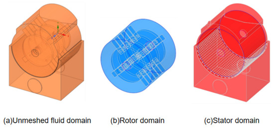
Figure 3.
Fluid domain model.
The method for extracting the flow field inside the pulverizer geometric model is to save the constructed geometric model in step format, import it into Ansys SpaceClaim 2021 R1 (Ansys, Inc., Canonsburg, PA, USA), and create “Inlet” and “Outlet” boundaries, with the “Inlet” boundary being the air inlet and the “Outlet” boundary being the rectangular area under the sieve, for model closure to extract the fluid field and subsequent solution settings using the Volume Extract function of SpaceClaim. Using the Volume Extract function in SpaceClaim, select the airflow inlet and outlet loop, extract the fluid domain, obtain the undivided fluid domain model, and establish the model coordinate system, the vertical direction as the Y-axis, the pulverizer axis as the Z-axis, and the origin located on the side of the rotary axis, as shown in Figure 3a.
Classification of the extracted fluid domain into dynamic and static domains. The dynamic domain corresponds to the cylindrical region swept by the rotor’s rotational motion. This cylindrical domain was constructed by aligning its central axis with the rotor’s rotational axis. A Boolean subtraction operation was then executed between the cylindrical volume and the rotor geometry to isolate the dynamic fluid domain, as depicted in Figure 3b. The resultant dynamic domain strictly adheres to the spatial envelope defined by the rotor’s rotation about its central axis. The static domain model was obtained by performing a Boolean subtraction operation between the global fluid domain and the dynamic subdomain (which encompasses the rotor-swept cylindrical region). This process excluded the rotating components, yielding the stationary fluid volume as illustrated in Figure 3c. Interface surfaces were established between the dynamic and static domains to enforce flow field continuity and facilitate robust data transfer of nodal solutions.
3. Numerical Simulation of Single-Phase Airflow
3.1. Fluid Domain Model Meshing
In CFD, mesh generation constitutes a foundational pillar of numerical modeling, as it governs the fidelity of flow field predictions and the reliability of derived engineering insights. In complex flow regimes characterized by steep gradients in velocity, pressure, and scalar transport variables, the spatial discretization scheme must resolve abrupt parametric transitions to ensure physical fidelity. Mesh refinement, while essential for enhancing simulation accuracy through improved resolution of flow gradients and boundary layer dynamics, imposes significant computational and storage overhead. By rational meshing, the computation and storage requirements can be minimized while satisfying the simulation accuracy.
Ansys Workbench Meshing Application 2021 R1 (Ansys, Inc., Canonsburg, PA, USA) is used for meshing, which guides the meshing process and has a higher degree of coupling with the Fluent solver. Poly-Hexcore mesh is used, which is a hybrid mesh with the advantages of polyhedral mesh and hexahedral mesh, which saves the computing power and ensures the accuracy of the calculation, and helps to shorten the calculation time and improve the efficiency. The mesh generation is shown in Figure 4.
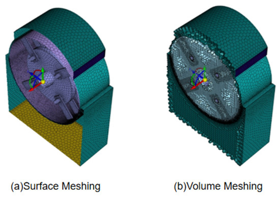
Figure 4.
Mesh generation.
3.2. Grid Independence Validation
In scenarios where the model details have achieved reasonable grid filling, increasing the number of grids may enhance calculation accuracy. However, once the grid reaches a certain density, further increasing the number of grids has limited impact on improving calculation precision, and excessive grid numbers can lead to unnecessary consumption of computational resources. To efficiently utilize computational resources, grid independence validation is performed.
Five groups of grids, ranging from 6.7 × 10⁵ to 1.35 × 10⁶, are selected for simulation under identical conditions. The static pressure at a specific point atop the crushing chamber is measured for grid independence validation. This approach ensures that the chosen grid density is sufficient for accurate simulations while avoiding overuse of computational resources.
Based on Table 2, when the grid count is between 1.06 × 10⁶ and 1.35 × 10⁶, the static pressure value stabilizes. Therefore, the grid scheme with 1.06 × 10⁶ grids is selected. In this configuration, the moving domain grid count is 3.2 × 10⁵, and the static domain grid count is 7.4 × 10⁵.
Table 2.
Mesh independence verification.
3.3. Solver and Boundary Settings
Due to the operating characteristics of the hammer mill, the rotor rotates to drive the airflow, and the flow field simulation for rotating machinery mostly adopts the Multi-Reference Frame (MRF) model, which utilizes the steady state (Steady) method to solve the rotor rotation as a constant problem at a certain moment, and establishes the local motion in each local computational region. In each local computational region, a local motion is established, and the flow field information in the local reference frame is transferred to the neighboring regions, so the multiple reference frame model is adopted. The Coupled algorithm in Fluent shows high efficiency and accuracy for rotational motion of incompressible fluids, and the Coupled algorithm is used for pressure–velocity basis coupling solution.
The specific parameters are set as follows:
- (1)
- The turbulence model adopted the Standard model with Standard Wall Functions (SWFs).
- (2)
- The inlet is set as a mass-flow-inlet and the outlet is set as a mass-flow-outlet in order to facilitate the calibration of the air inlet volume.
- (3)
- The fluid material is set to AIR and a gravitational acceleration along the opposite direction of the Y-axis is applied.
- (4)
- The reference system of the dynamic domain is set as rotating reference system, the direction of rotation is around the Z-axis, and the connecting surface between the dynamic and static domains is set as the interface intersection. The rotor is set as a moving wall, following the neighboring mesh motion, and the relative velocity is set to 0.
- (5)
- The coupled pressure–velocity basis is solved using the Coupled algorithm, with second-order interpolation for pressure and first-order windward discretization for momentum and energy equations.
3.4. Flow Field Simulation Test Design
According to the production experience, the hammer blade end line speed is generally about 60–100 m/s; from the rotor shaft, the hammer blade size can be calculated to obtain the rotor speed. Considering the production experience and the working performance of the pulverizer, the rotor speed levels were set to three levels of 1700 r/min, 2500 r/min, and 3300 r/min.
Set the inlet boundary conditions for the mass flow into the mouth, that is, by setting the air mass flow parameters to change the inlet air volume. At the same time, under the condition that the shape of the crushing chamber remains unchanged, the fan air volume is calculated according to the hammer mill screen area of 2600–3500 m3/(h-m2), and the air volume should be about 1500 m3/h as calculated from the effective screen area.
Using an anemometer to measure the value of airflow velocity at the air inlet under the fan open condition, the average airflow velocity range of the air inlet was obtained as 0 to 9.7 m/s, the area of the air inlet was about 0.06 m2, and the air inlet volume formula is as follows:
where is volumetric airflow rate (m3/h), is cross-sectional area of the intake (m2), and V is airflow velocity (m/s).
The experimentally measured volumetric airflow rate (L) within the grinding system was determined to range from 0 to 2095 m3/h. To systematically evaluate airflow-dependent performance, four discrete airflow levels were defined: 0 m3/h, 1000 m3/h, 1500 m3/h, and 2000 m3/h. Based on the standard air density (ρ = 1.293 kg/m3 at 25 °C and 101.325 kPa), the mass flow rate levels for the intake airflow were systematically assigned as 0 kg/s, 0.36 kg/s, 0.54 kg/s, and 0.72 kg/s.
In order to accurately describe the variation in the flow field characteristics in the pulverizing chamber under different rotor speeds and air inlets, three different macroscopic cross-sections were selected according to the working characteristics of the pulverizer. As shown in Figure 5, the P1 cross-section is located at the Z = 178.79 mm plane to observe and analyze the radial flow along the rotor; the P2 cross-section is located at Y = 0 plane to observe and analyze the axial flow along the rotor; the P3 cross-section is located at the inner sieve surface to observe the sieve area flow. These three sections can be more comprehensive expressions of the macroscopic pressure field and the velocity field characteristics of the pulverizing cavity flow field.
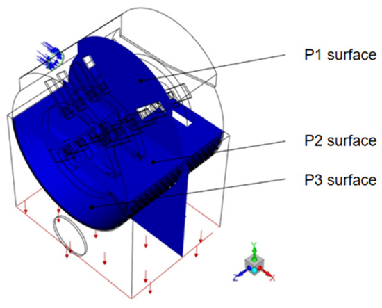
Figure 5.
Distribution of observed cross-sections.
At the same time, in order to deeply study the influence on the screening process under different rotor speeds and air intakes, as shown in Figure 6, macroscopically selected area I (the gap between the hammers and the sieve surface), microscopically selected area II (inside the designated sieve holes), and LINE (4 mm line inside and outside the bottom sieve holes) were used as the objects of the study.
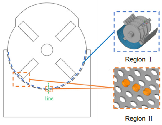
Figure 6.
Distribution of observation areas.
4. Results of Single-Phase Airflow
4.1. Analysis of the Influence of Rotor Speed on Flow Field Characteristics
4.1.1. Pressure Field Analysis at Different Speeds
Hammer mill internal pressure field distribution is an important part of the flow field study; static pressure affects the material perforation force, dynamic pressure affects the speed of the material perforation, and the screen surface inside and outside of the pressure difference can be judged by the difficulty of the material over the screen.
Figure 7 shows the static pressure variation curves along the inner and outer sides of the rotor radial sieve surface (without passing through the sieve holes) at three rotor speeds without an applied wind field, and the blue area is the location of the sieve surface.
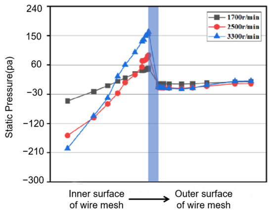
Figure 7.
Variation in static pressure inside and outside the screen surface at different rotor speeds.
Due to the rotor fan effect, there will be negative pressure at the center of the rotor; the static pressure value at the surface of the rotor shaft is the smallest, and the static pressure value along the radial direction of the rotor gradually increases. The higher the rotor speed, the greater the static pressure value near the inner side of the screen surface, while the outer side of the screen surface static pressure changes are smaller, the maximum static pressure difference between the inner and outer sides of the screen surface of the three rotor speeds are 46.93 Pa, 98.95 Pa, 170.21 Pa, respectively.
The static pressure difference formed by the rotor fan effect makes the crushed straw particles have the tendency to move to the center of the rotor, which is unfavorable for screening, while the static pressure difference formed between the inner and outer sides of the sieve surface points to the outer side of the sieve surface from the inner side of the sieve surface (the static pressure of the inner surface of the sieve surface is higher than the static pressure of the outer side of the sieve surface), which is favorable for screening. However, it is obvious that the maximum static pressure difference between the inner and outer sides of the screen surface is much smaller than the maximum static pressure difference due to the effect of the rotor fan in the absence of a fan, so it is difficult to form the static pressure difference between the inner and outer sides of the screen surface that is favorable for the sieving of crushed straw particles by relying on the increase in rotor rotation speed alone.
4.1.2. Velocity Field Analysis at Different Rotational Speeds
Figure 8 shows the velocity cloud of the P1 plane at three rotor speeds. In the rotor sweep area, the minimum airflow velocity appears at the surface of the rotor shaft, along the radial direction of the rotor; the airflow velocity gradually increases, the maximum airflow velocity is found at the edge of the end of the hammer blade, and the airflow velocity gradually decreases from the end of the hammer blade to the inner surface of the screen surface. With the increase in rotor speed, the maximum value of airflow velocity in the P1 plane increases, and the maximum values of airflow velocity at the three rotor speeds are 56.71 m/s, 82.30 m/s, and 109.43 m/s, respectively.
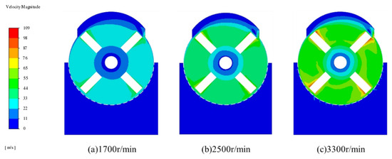
Figure 8.
Plane velocity cloud of P1 at different rotor speeds.
The velocity field in Region I (reference zone) was analyzed, with Figure 9 illustrating the velocity vector distributions under three rotor speeds. A subset of airflow exhibited reverse flow toward the rotor center due to the rotor’s fan effect. The measured reverse flow velocities were as follows: 1700 rpm (151.8 rad/s): 5.23–7.65 m/s, 2500 rpm (261.8 rad/s): 6.11–9.58 m/s, 3300 rpm (345.6 rad/s): 12.17–15.43 m/s.
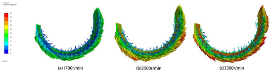
Figure 9.
Velocity vector diagram of region I at different rotor speeds.
The results confirm a positive correlation between rotor speed and reverse flow intensity, indicating enhanced fan effects at higher rotational speeds.
To investigate the influence of rotor speed on airflow patterns near generic screen apertures, streamline plots were generated for the three rotor speeds at a bottom screen region distal to the hammer tips (Figure 10).
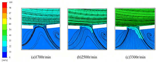
Figure 10.
Streamline distribution of sieve holes at the bottom of region II at different rotor speeds.
As shown in Figure 10, streamline distributions of airflow through the screen apertures differ significantly under the three rotor speeds. At higher rotor speeds, fewer streamlines enter the apertures despite an equivalent number of streamlines passing above the screen. This occurs because the higher tangential airflow velocity in the annular boundary layer at elevated rotor speeds increases the difficulty of altering its tangential motion direction, thereby reducing airflow penetration into the apertures.
To accurately characterize airflow velocity variations near the bottom screen apertures, the airflow velocity profiles on both the inner and outer sides of the designated line position were plotted under varying rotor speeds, as shown in Figure 11.
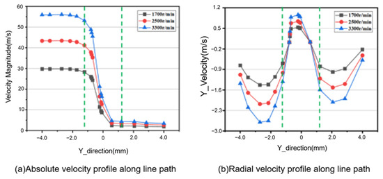
Figure 11.
Variation in airflow velocity along line at different rotor speeds.
In Figure 11a, the curves illustrate the variation in absolute airflow velocity from the inner to outer surfaces of the bottom screen apertures, with the dashed-line demarcated zone corresponding to the interior of the screen apertures. At the inner screen surface, the absolute airflow velocity remained constant, approximating the annular boundary layer airflow velocity correlated to the respective rotor speeds. Within the apertures, the absolute airflow velocity progressively decreased, reaching stabilized values of 2.21 m/s, 3.30 m/s, and 4.38 m/s under the three rotor speeds. At the outer screen surface, the absolute airflow velocity remained consistently low and stable.
Figure 11b depicts the radial airflow velocity profile, with the outward direction through the screen defined as the positive velocity direction. On the inner screen surface, the radial velocity initially increases and then decreases, remaining significantly lower than the absolute airflow velocity. This demonstrates that the tangential airflow velocity dominates the radial component (as the absolute velocity is derived from the vector sum of tangential and radial velocities), with the radial flow direction oriented toward the rotor center; within the screen apertures, the radial airflow velocity decreases to zero before reversing direction and increasing. Higher rotor speeds amplify the overall radial through-screen airflow, with peak velocities measured at 0.54 m/s (1700 rpm), 0.74 m/s (2500 rpm), and 0.96 m/s (3300 rpm). Post-peak, the velocity gradually diminishes.
4.2. Analysis of the Influence of Intake Air Volume on Flow Field Characteristics
4.2.1. Pressure Field Analysis at Different Air Inlet Volumes
The static pressure variation curves along the inner and outer surfaces of the radial bottom screen (avoiding apertures) under the three airflow rates are shown in Figure 12, with the screen position marked by the blue zone. The maximum static pressure differentials between the inner and outer screen surfaces were measured as 201.02 Pa, 256.27 Pa, and 284.36 Pa under increasing airflow rates, compared to a baseline differential of 98.95 Pa without forced airflow. This demonstrates a clear trend: the maximum static pressure differential across the screen increases with higher airflow rates. The forced airflow significantly increased the static pressure at the rotor surface. The maximum static pressure differentials from the inner bottom screen surface to the rotor shaft surface were measured as 1701.39 Pa, 1302.92 Pa, and 992.53 Pa under the three airflow rates, compared to 2187.45 Pa without forced airflow. This demonstrates an inverse relationship: for every 500 m3/h increase in airflow rate, the maximum static pressure differential decreased by approximately 400 Pa.
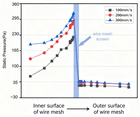
Figure 12.
Variation in static pressure difference between inside and outside the screen surface with different air inlet volume.
4.2.2. Velocity Field Analysis with Different Air Intake
As shown in Figure 13, P1-plane velocity contours under three airflow rates at a rotor speed of 2500 rpm exhibit similar macroscopic characteristics. The maximum airflow velocity occurs at the trailing edges of the hammer tips, reaching the tip linear velocity of the hammers. Compared to the configuration without forced airflow, the velocities near the inlet and through the screen apertures are significantly amplified, with further increases observed as the airflow rate rises.
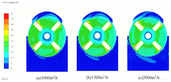
Figure 13.
Plane velocity cloud of P1 with different inlet air volume.
Within the air-material annular flow layer, the motion of suspended particles is driven by circumferential airflow, resulting in a reduced linear velocity differential between straw particles and hammers. This diminished velocity gradient adversely impacts grinding effectiveness by weakening impact forces and shear stresses during particle–hammer interactions. The introduction of forced airflow reduces the airflow velocity within the annular flow layer. Assuming negligible changes in the circumferential airflow direction, this configuration theoretically increases the linear velocity differential between straw particles and hammers, potentially enhancing grinding efficiency. This hypothesis, however, represents a simplified model that neglects critical factors such as airflow vector orientation and secondary flow patterns. Definitive evaluation of grinding performance impacts necessitates detailed velocity field analysis to quantify the spatial distribution of velocity gradients and particle trajectories.
The tangential and radial velocities of airflow in Region I were calculated using volume-weighted averaging across varying airflow rates. Table 3 presents the mean tangential and radial velocities of airflow in Region I at a rotor speed of 2500 r/min under different airflow supply conditions.
Table 3.
Average velocity of Region I under different air inlet volume.
As indicated in Table 3, the forced airflow induces a reversal of radial velocity from negative (directed toward the rotor center) to positive (outward through the screen), with its magnitude increasing proportionally to airflow rate. Concurrently, the tangential velocity decreases as airflow rate rises. Nonuniform velocity distribution in Region I reveals that the peak tangential velocity within the annular flow layer reaches approximately 1.5 times the mean tangential velocity (calculated from sampled data). This velocity configuration—reduced tangential velocity combined with elevated radial velocity—enhances particle screening efficiency by minimizing centrifugal retention forces (which scale with tangential velocity) while amplifying normal momentum transfer (linked to radial velocity magnitude).
Further investigation into the tangential and radial airflow velocities in Region I under varying rotor speeds revealed that radial velocities showed no significant variation across different rotor speeds at a fixed airflow rate. For tangential velocities, a bivariate linear regression model incorporating rotor speed and airflow rate demonstrated strong predictive capability, with a coefficient of determination (R2) of 0.91582, indicating excellent model fit. This statistical relationship quantitatively characterizes the dependency of tangential airflow dynamics on both operational parameters.
where is rotor speed (rpm), is airflow rate (m3/h), and is tangential airflow velocity (m/s).
Figure 14 illustrates the internal streamline patterns of bottom screen apertures in Region II under three airflow rates, with dashed lines demarcating airflow entering the apertures. With forced airflow activation, the proportion of screen aperture width traversed by airflow significantly increased. Notably, the incremental airflow penetration from 1000 to 1500 m3/h was substantially greater than that observed from 1500 to 2000 m3/h, indicating diminishing returns in aperture utilization efficiency at higher airflow rates.
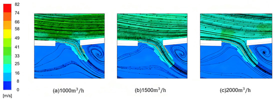
Figure 14.
Variation in sieve flow lines at the bottom of Region II under different air inlet volumes.
Dynamic principles were applied to analyze this phenomenon: when airflow moves from above the inner screen surface toward the apertures with an initial velocity vector aligned tangentially to the screen surface, the airflow enters the aperture with a tangential initial velocity V. Subject to an external airflow force acting over a duration, the airflow’s entry angle into the aperture can be expressed as follows:
The variation in airflow entry angle with respect to applied force can be expressed as follows:
where is airflow entry angle (°), is external airflow force (N), is interaction duration (s), and is initial tangential airflow velocity (m/s).
The airflow entry angle critically determines the aperture throughput capacity. As demonstrated by Equations (16) and (17), increasing the airflow rate amplifies the external airflow force, which elevates the entry angle. However, the angular increment rate diminishes progressively with higher airflow rates. This nonlinear relationship theoretically explains the observed deceleration in airflow penetration enhancement at elevated airflow rates, where geometric constraints of screen apertures and saturation of tangential-to-normal momentum conversion jointly limit further throughput gains.
Figure 15 displays the airflow velocity profiles along a designated line from the inner to outer screen surfaces at the bottom sieve apertures under three airflow rates, with the rotor operating at 2500 rpm. The curves quantify how airflow velocity evolves spatially under varying forced-air conditions. The observed reduction in total airflow velocity at the inner screen surface with increasing airflow rate experimentally validates the suppressive effect of forced airflow on annular flow layer dynamics. Comparative analysis reveals that airflow rate exerts less influence on bulk airflow velocity than rotor speed variations, indicating that rotor-driven centrifugal forces dominate the macroscopic airflow scaling within the comminution chamber. Increasing airflow rate significantly enhances the radial screening airflow velocity within the apertures, with a more pronounced impact compared to rotor speed variations. Specifically, the maximum radial screening velocities under three airflow rates were measured as 1.94 m/s, 3.44 m/s, and 4.31 m/s, demonstrating a nonlinear amplification effect.
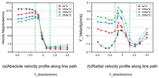
Figure 15.
Variation in airflow velocity along line with different inlet airflow rates.
5. Numerical Simulation of CFD-DEM Coupling
5.1. Coupling Model Assumptions
In order to solve the strong interaction between straw particles and airflow and particles, Fluent-EDEM is used for bidirectional coupling transient calculation in this study. In view of the significant influence of particle volume fraction on the screening process, the Euler–Eulerian model, which can fully reflect the particle-phase volume fraction, is selected instead of the Euler–Lagrange model that only considers momentum exchange.
5.2. Coupling Simulation Calculation Model
5.2.1. Calculation Domain Model of the Pulverizer
The computational domain for EDEM has been modified from the fluid domain, converting the inlet and outlet into wall boundaries, and changing the interface to interior. The mesh configuration remains consistent with Fluent to ensure seamless data exchange. The models for the computational domains of both are depicted in Figure 16.
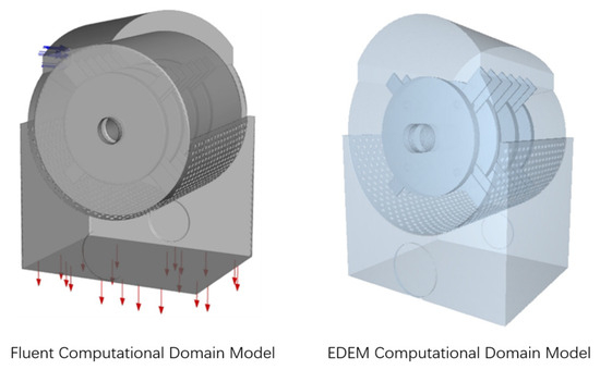
Figure 16.
Computational domain model.
5.2.2. Key Parameter Settings
Fluent: A transient solver is utilized, along with the sliding mesh method and the SIMPLE algorithm. The time step is set to 1.1 × s, and the Eulerian multiphase flow model is activated.
EDEM: The time step is set to 2.2 × s (approximately 1/50 th of Fluent’s time step). The straw model is represented as a cylinder (20 mm in length and 9 mm in diameter) filled with multi-scale spherical particles, connected by 2957 particles through 8441 bonded contacts. This study references and researches the properties of vine stem-like straw [4]. The key material parameters and contact parameters are detailed in Table 4.
Table 4.
Parameters of intrinsic and contact.
5.3. Numerical Simulation of the Crushing Process
By comparing the crushing processes at three different rotational speeds—1700, 2500, and 3300 r/min—it is observed that at lower speeds, the hammer primarily exhibits a cutting effect on the straw. As the rotational speed increases, the kinetic energy of the hammer rises, resulting in a more complex crushing pattern (as shown in Figure 17). Rotor speed is a critical factor influencing the crushing effect.
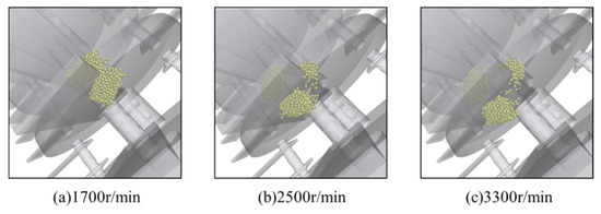
Figure 17.
Schematic diagram of straw crushing under varying speeds.
To quantify the airflow impact, the relative velocity between the hammer tip and suspended particles was estimated as expressed by the following equation. Calculations indicate that without a fan, the relative velocity at 2500 r/min is approximately 66 m/s. Simulations revealed that at identical relative velocities (i.e., by adjusting the combination of rotational speed and air intake volume), the agglomeration bond breakage rate under airflow conditions (1500 m3/h) was higher (91.24%) than under non-airflow conditions (84.30%). This confirms that the fan-generated airflow enhances the pulverization process.
where is the relative velocity between the hammer tip and suspended particles, m/s; is the linear velocity of the hammer tip, m/s; is the rotor speed, r/min; and is the airflow rate, m3/h.
Further analysis of the coupling forces reveals that as the inlet airflow increases, the coupling force between the straw and the air also increases. Although this force is significantly smaller than the mechanical contact force, during the rubbing and crushing stage, airflow disturbances can still promote the crushing process by altering the motion state of the particles (as illustrated in Figure 18).
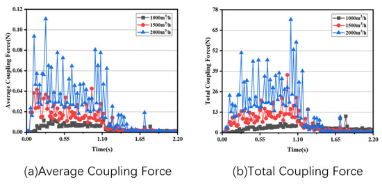
Figure 18.
Variation in air–straw coupling force.
5.4. Numerical Simulation of the Screening Process
5.4.1. Design of Simulation Experiments for the Screening Process
In this section, a CFD-DEM coupling method is used to analyze the screening process of the straw discrete element model, investigating the impacts of rotor speed, inlet airflow, and feed rate on the screening process of a hammer mill. Since, in actual screening processes, materials that meet the screening conditions may not pass through due to certain reasons, this section focuses on the ability of materials smaller than the screen openings to effectively pass through the screen surface without considering the specific crushing process.
During this phase, particles are continuously generated from 0 to 3 s, with no particle generation from 3 to 5 s. The areas above and below the screen surface are the objects of study. The particle model used in the screening process simulations is simplified from a bonded model of smaller particles to cylindrical particles, and all generated straw particle diameters are smaller than the screen opening diameter. The particle size distribution within the crushing chamber can be well described by the Rosin-Rammler size distribution model, with the characteristic size set to 3 mm.
5.4.2. Single Factor Analysis
Simulations of the screening process under conditions without fan influence and a particle filling rate of 0.4 kg/s were performed at three different rotor speeds, as shown in Figure 19. The screening rate decreases with increasing rotor speed (67.72% at 1700 r/min and 61.09% at 3300 r/min). High rotor speeds enhance the centrifugal effect on particles, which is unfavorable for screening.
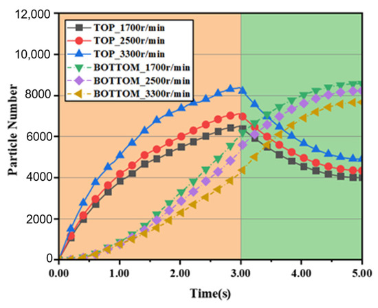
Figure 19.
Variation in particle number in two regions under varying speeds.
At a rotor speed of 2500 r/min and a particle filling rate of 0.4 kg/s, simulations at three different airflow volumes were conducted, as illustrated in Figure 20. An inlet airflow of 1500 m3/h resulted in the highest screening rate (88.10%), while rates that were too low or too high led to a decrease in screening efficiency.
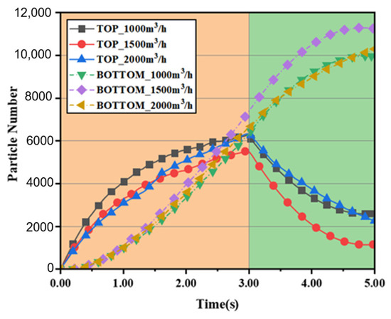
Figure 20.
Variation in particle number in two regions under varying airflow rates.
Under conditions of rotor speed at 2500 r/min and inlet airflow at 1500 m3/h, simulations of the screening process were carried out at three different particle filling rates, as shown in Figure 21. The screening rate decreases as the feed rate increases (92.12% at 0.25 kg/s and 79.03% at 0.55 kg/s), although the total number of particles screened increases.
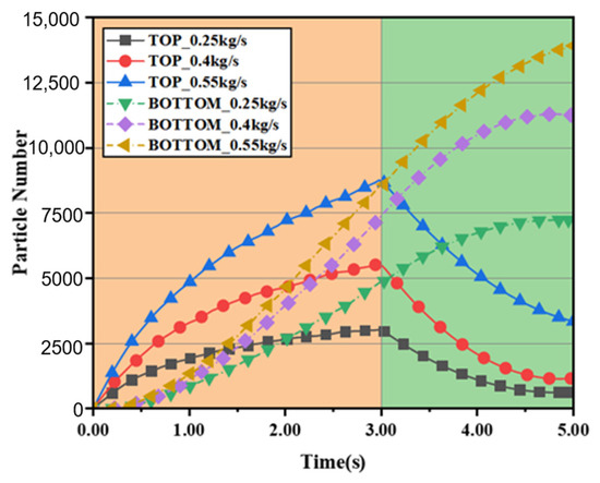
Figure 21.
Particle number variation in two regions under varying particle filling rates.
5.4.3. Orthogonal Experimental Design
An L9(33) orthogonal table was adopted, with three factors and three levels as follows:
A (Rotor Speed): 1700, 2500, 3300 r/min
B (Inlet Airflow): 1000, 1500, 2000 m3/h
C (Feed Rate): 0.25, 0.4, 0.55 kg/s
Table 5 presents the detailed orthogonal experimental design scheme and simulation results.
Table 5.
Design and results of orthogonal experiment.
5.4.4. Analysis of Orthogonal Experiment Results
- (1)
- Range Analysis
Table 6 indicates that the order of influence of each factor on the screening rate is as follows: inlet airflow (B) > feed rate (C) > rotor speed (A). The optimal combination is A1B2C1.
Table 6.
Range analysis table.
- (2)
- Variance Analysis
Table 7 further confirms that inlet airflow (B) and feed rate (C) have significant effects on the screening rate (p value < 0.05), while the effect of rotor speed (A) is not significant.
Table 7.
ANOVA Table.
6. Field Test
6.1. Experimental Plan
Productivity () and energy consumption per ton () are the primary indicators, with average particle size () as an auxiliary indicator. A three-factor, five-level second-order orthogonal rotational composite design was employed, with the factor-level encoding shown in Table 8. A total of 23 factor-level combinations were derived, and the experimental results are depicted in Table 9.
Table 8.
Factor level table.
Table 9.
Quadratic regression orthogonal rotatable composite design and results.
6.2. Result Analysis and Regression Model
6.2.1. Analysis of the Effects of Factors on Productivity
- (1)
- Multivariate regression analyses were performed on the orthogonal experiment results, resulting in the regression equation for productivity as follows:
Table 10 summarizes the ANOVA results for the productivity regression, assessing the overall significance of the model.
Table 10.
ANOVA of the productivity regression equation.
The regression model is highly significant (p < 0.0001) and demonstrates a good fit. Analysis indicates that rotor speed (X1), feed rate (X3), and their quadratic terms are extremely significant factors affecting productivity (Y1). Inlet airflow (X2) and its interaction with rotor speed (X1X2) also have significant effects. After removing insignificant quadratic terms, the regression equation is as follows:
- (2)
- Analysis of the Interaction Effects of Factors on Productivity
When the feed rate is fixed at 6 kg/min, the response surface plot illustrating the impact of rotor speed and fan aperture on productivity is shown in Figure 22a. Productivity increases as both rotor speed and fan aperture increase, with an optimal inlet airflow observed.
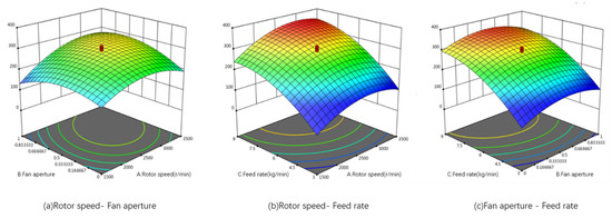
Figure 22.
Response surface analysis of the interaction effects on productivity.
When the fan aperture is fixed at 50%, the response surface plot showing the impact of rotor speed and feed rate on productivity is represented in Figure 22b. In actual experiments, productivity increases with higher rotor speeds and feed rates, although significant inefficiencies are observed at lower speeds.
When the rotor speed is fixed at 2500 r/min, the response surface plot of fan aperture and feed rate impacting productivity is depicted in Figure 22c. Here, productivity initially increases with fan aperture before decreasing, revealing a clear trend of change.
6.2.2. Analysis of the Impact of Various Factors on Power Consumption
- (1)
- Construction and Significance Testing of the Energy Consumption per Ton Regression Model.
After computations, the regression equation for energy consumption is obtained as follows:
Table 11 summarizes the ANOVA results for the productivity regression, assessing the overall significance of the model.
Table 11.
ANOVA of the power consumption per ton regression equation.
The regression model for energy consumption per ton (Y2) is highly significant (p < 0.0001), with a good fit and high reliability. Analysis reveals that rotor speed (X1), inlet airflow (X2), feed rate (X3), and the quadratic terms of all factors have a highly significant impact on energy consumption per ton. The interaction term X1X3 has a significant effect, while X1X2 and X2X3 are not significant. The lack of fit is not significant (p > 0.05), further confirming that the model fits the experimental data well. After removing the insignificant interaction terms, the regression equation is as follows:
- (2)
- Analysis of the Interaction Effects of Factors on Energy Consumption
When the feed rate is fixed at 6 kg/min, the response surface plot showing the impact of rotor speed and fan aperture on energy consumption per ton can be observed in Figure 23a. It indicates that at rotor speeds between 2100 and 2700 r/min and fan apertures between 49% and 85%, energy consumption per ton is relatively low. With further increases in rotor speed and fan aperture, energy consumption initially increases before decreasing.
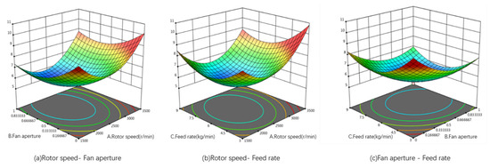
Figure 23.
Response surface analysis of the interaction effects on power consumption.
When the fan aperture is fixed at 50%, the response surface plot illustrating the effect of rotor speed and feed rate on energy consumption per ton, shown in Figure 23b, reveals that energy consumption is low at rotor speeds between 2000 and 2600 r/min and feed rates between 5.3 and 7.5 kg/min. As both rotor speed and feed rate increase further, energy consumption initially increases again before decreasing.
When the rotor speed is set at the zero level, i.e., 2500 r/min, the response surface plot depicting the influence of fan aperture and feed rate on energy consumption per ton, as seen in Figure 23c, indicates that energy consumption is lower with fan apertures between 55% and 83% and feed rates between 5.4 and 7.7 kg/min. Similarly, further increases in rotor speed and feed rate show the same trend of energy consumption first increasing and then decreasing.
The average particle size is not considered a performance indicator in this study but is utilized as an auxiliary metric to explore the relationship between various factors and the crushing and screening characteristics, and thus it is not analyzed in detail.
6.3. Parameter Optimization and Validation Experiment
Using Design Expert 13 (Stat-Ease, Inc., Minneapolis, MN, USA) software, parameter optimization was carried out with the goal of maximizing productivity Y1 and minimizing energy consumption per ton Y2. By combining these objectives with the boundary conditions of each factor and maintaining constant structural parameters of the crusher, an optimized model for three working parameter combinations was obtained as follows:
The optimization results show that when the rotor speed is 2569 r/min, the fan aperture is 62.55%, and the feed rate is 7.64 kg/min, the crusher achieves its best working performance. Under these conditions, the productivity is 337 kg/h, and the energy consumption is 5.59 kW·h/t.
To validate the optimization results, three repeated verification experiments were conducted under the same test conditions as before. These conditions maintain a rotor speed of 2569 ± 30 r/min, a fan aperture of 62.55 ± 3%, and a feed rate of 7.64 kg/min. The experimental results are presented in Table 12.
Table 12.
Optimization parameter validation and error.
The comparison reveals that the actual productivity values deviate less than 6% from the theoretical values, and the actual energy consumption per ton values deviate less than 3% from the theoretical values. This demonstrates a high level of consistency between the actual and theoretical results, confirming the reliability of the optimization model and its effectiveness in achieving desired operational performance in the crushing process.
7. Discussion
The present study demonstrates that the introduction of controlled external airflow significantly enhances both crushing efficiency and screening performance in hammer mill processing of cucumber straw, a tough and fibrous agricultural biomass. While previous studies have largely focused on rotor-induced airflow or screen geometry modifications [8,10], our integrated approach, combining CFD analysis, coupled CFD-DEM simulations, and field experiments, quantitatively establishes that an optimal external airflow rate (around 1500 m3/h) can fundamentally alter the particle–fluid dynamics within the comminution chamber to improve overall system performance.
A key finding is the non-monotonic relationship between airflow rate and screening efficiency, which peaks at a specific flow rate rather than increasing indefinitely. This can be explained by the competing effects of airflow on particle transport. At lower rates, the forced airflow sufficiently reduces the tangential velocity of the particle–airflow annular layer (Table 3), thereby diminishing the centrifugal force that retains particles against the screen. However, as the airflow increases beyond the optimum, excessive radial momentum may lead to particle re-entrainment or turbulent fluctuations that disrupt the orderly passage of particles through the screen apertures, as observed in the streamline analysis of Region II (Figure 14). This phenomenon aligns with the findings of Qian et al. [8], who reported that screen geometry alone could not fully address the issue of material retention without considering auxiliary airflow.
Furthermore, the regression model derived from field tests (Equation (20)) underscores that feed rate (X3) is the most influential factor affecting productivity, followed by rotor speed (X1) and airflow (X2). This hierarchy of operational parameters provides a clear, practical guideline for industrial system optimization. The significant interaction effect between rotor speed and airflow (X1X2) further implies that these parameters should not be tuned independently—a critical consideration not thoroughly addressed in earlier hammer mill studies such as those by Budăcan et al. [9].
From a mechanistic perspective, the CFD results revealed that external airflow serves a dual purpose. It not only enhances particle–screen impingement by increasing the radial through-screen velocity (Figure 15) but also counteracts the adverse negative pressure gradient induced by the rotor’s fan effect. This mitigation of backflow near the screen holes—a phenomenon also noted by Zhang et al. [10] in corn stover crushers—creates a more favorable pressure differential for screening (Figure 12). Our coupled CFD-DEM simulations provide a deeper confirmation: while the primary breakage mechanism remains impact-based, the aerodynamic forces help reposition particles, increasing the probability of high-impact, shattering collisions with the hammers and reducing energy-intensive rubbing and friction, as evidenced by the higher bond breakage rate under optimal airflow.
Despite these insights, this study has certain limitations. The DEM simulations for the screening process assumed spherical particles for computational efficiency, whereas actual straw fragments are irregular and fibrous, which may influence interlocking and screening behavior. Future work should incorporate non-spherical DEM models to better represent straw morphology. Additionally, the current model does not fully account for the effects of variable moisture content—a critical factor in real-world straw processing—on both breakage behavior and airflow interaction.
In a broader context, this research validates the use of integrated CFD-DEM modeling as a powerful tool for deconstructing and optimizing the complex multi-physics processes in biomass comminution. The methodology and insights demonstrated here, particularly on the interaction between operational parameters, can be extended to the processing of other fibrous agricultural residues, supporting the development of more efficient, lower-energy, and precisely controlled systems for sustainable agriculture.
8. Conclusions
CFD simulations were employed to systematically investigate the airflow field distribution within the comminution chamber under varying rotor speeds and airflow rates. These simulations revealed the governing mechanisms of both parameters on airflow characteristics through macro-scale flow structures and micro-scale turbulence parameters.
Under natural airflow conditions (no forced air supply), increasing rotor speed significantly amplifies the maximum static pressure differential between the inner screen surface and rotor shaft surface, intensifying wall impact losses. The peak airflow velocity within the annular flow layer remains consistently proportional to the hammer tip linear velocity, stabilizing at approximately 70% of its value. Along the screen surface, airflow predominantly follows tangential trajectories, with only a small portion passing through the screen apertures. Microscopic analysis reveals localized backflow phenomena near screen apertures adjacent to hammer tips. Vortices generated on the screen surface reduce airflow velocities, while the maximum radial screening airflow velocity inversely correlates with the proportion of airflow exiting through the apertures. Reduced airflow penetration enhances localized momentum focusing, thereby elevating peak radial velocities.
Under constant rotor speed conditions, increasing the airflow rate induces systematic modifications to both macroscopic and microscopic airflow dynamics. Macroscopically, the axial static pressure gradient diminishes progressively while developing irregular distribution patterns. The static pressure differential between the inner screen surface and rotor center decreases with higher airflow rates, and the positive pressure values on the screen exhibit significant deviations from those observed under natural airflow (no forced ventilation). Notably, elevated airflow rates reduce the rotor-induced static pressure differential (attributed to the fan effect) while amplifying the static pressure gradient across the screen (inner vs. outer surfaces). This enhanced cross-screen pressure gradient facilitates the penetration of crushed straw particles through apertures by intensifying normal momentum transfer.
Using a coupled CFD-DEM model, this study reveals that cucumber vine straw crushing is primarily governed by mechanical impact rather than airflow. For screening, the airflow rate is the most significant factor, exhibiting a non-monotonic relationship with efficiency, while increased particle feed rate nonlinearly influences specific impulse, indicating shifting power consumption.
An experimental study was conducted to investigate the crushing and screening characteristics of cucumber vine straw and to optimize the operational parameters. A three-factor, five-level central composite rotatable design was employed, and separate quadratic regression models were established. The results demonstrated that external airflow disturbance significantly enhances crushing efficiency. Furthermore, the influence of various factors on production rate, energy consumption per ton, and average particle size was elucidated. The experimental findings showed good agreement with the numerical simulations.
Author Contributions
Conceptualization, L.H., X.Z. (Xiujing Zhao) and L.R.; methodology, L.H., X.Z. (Xiujing Zhao) and L.R.; software, X.Z. (Xiujing Zhao) and L.R.; validation, L.H. and X.Z. (Xiujing Zhao); formal analysis, Y.X.; investigation, X.Z. (Xiliang Zhang) and Y.X.; writing—original draft preparation, L.H.; writing—review and editing, X.Z. (Xiliang Zhang); visualization, X.Z. (Xiliang Zhang); supervision, Y.X. and X.Z. (Xiliang Zhang); project administration, Y.X. All authors have read and agreed to the published version of the manuscript.
Funding
This work was supported by the Technology Development Project of Leo Group Co., Ltd. (Taizhou, Zhejiang, China) (HX20230724) and Project of Jiangsu Province Postdoctoral Research Funding Program (2021K086A).
Data Availability Statement
The raw data supporting the conclusions of this article will be made available by the authors on request.
Conflicts of Interest
The authors declare no conflicts of interest.
Abbreviations
| Abbreviations | |
| CFD | Computational Fluid Dynamics |
| DEM | Discrete element method |
| DPM | Dense Phase Model |
| RANS | Reynolds-averaged Navier–Stokes |
| MRF | Multi-Reference Frame |
| SWF | Standard Wall Functions |
| Nomenclature | |
| Fluid density constant | |
| Flow time | |
| uy, uz | The components of the fluid velocity in the direction of , and . |
| Hydrostatic pressure acting on the fluid element | |
| Viscous stress tensor components (i = n: normal direction, j = t: tangential direction) | |
| , Fy, | Cartesian components of body force per unit mass |
| Force exerted by straw pellets on the airflow | |
| Volume of the fluid element mesh | |
| The mass of the straw particle, kg | |
| The velocity of the straw particle, m/s | |
| The contact force acting on the straw particle, N | |
| The force exerted by the airflow on the straw particle, N | |
| The rotational inertia of the straw particle, kg·m2 | |
| The angular velocity of the straw particle, rad/s | |
| The torque generated by the contact force, N·m | |
| The torque generated by the airflow acting on the straw particle, N·m | |
| The drag coefficient | |
| The particle diameter, m | |
| The air density, taken as 1.29 kg/m3 | |
| The tangential and normal cohesive force, N | |
| The tangential and normal cohesive stress moment, N·m | |
| The particle tangential and normal velocity, m/s | |
| The unit area tangential and normal stiffness, N/m | |
| The cohesive bond cross-sectional area, m2 | |
| The moment of inertia, kg·m2 | |
| Time step, s | |
| The bond radius, m | |
| The critical stress in the tangential and normal directions, Pa | |
| Dimensionless empirical constants (not flow variables) that act as effective turbulent Prandtl numbers, | |
| The flow length and velocity in the direction | |
| The production of turbulent kinetic energy due to mean velocity gradients | |
| Volumetric airflow rate (m3/h) | |
| Cross-sectional area of the intake (m2) | |
| V | Airflow velocity (m/s) |
| Rotor speed (rpm) | |
| Airflow rate (m3/h) | |
| Tangential airflow velocity (m/s) | |
| Airflow entry angle (°) | |
| External airflow force (N) | |
| Interaction duration (s) | |
| Initial tangential airflow velocity (m/s) | |
| The relative velocity between the hammer tip and suspended particles, m/s | |
| The linear velocity of the hammer tip, m/s | |
| A1, A2, A3 | Rotor speed constant |
| B1, B2, B3 | Inlet airflow constant |
| C1, C2, C3 | Feed rate constant |
| Productivity (kg/h) | |
| Energy consumption per ton (kW · h/t) | |
| Average particle size (mm) | |
| X1 | Rotor speed (r/min) |
| X2 | Damper opening |
| X3 | Feed rate (kg/min) |
References
- Dong, J.X.; Cao, H.Y.; Zhu, Y.Y. Research progress of straw energy utilization technology based on Citespace analysis. World Sci. Technol. Res. Dev. 2023, 45 (Suppl. 1), 71–87. [Google Scholar]
- Xu, Y.F.; Zhang, X.L.; Sun, X.J.; Wang, J.Z.; Liu, J.Z.; Li, Z.G.; Guo, Q.; Li, P.P. Tensile Mechanical Properties of Greenhouse Cucumber Cane. Int. J. Agric. Biol. Eng. 2016, 9, 1–8. [Google Scholar]
- Wang, X.; Tian, H.; Xiao, Z.; Zhao, K.; Li, D.; Wang, D. Numerical Simulation and Experimental Study of Corn Straw Grinding Process Based on Computational Fluid Dynamics–Discrete Element Method. Agriculture 2024, 14, 325. [Google Scholar] [CrossRef]
- Guo, Q.; Zhang, X.; Xu, Y.; Li, P.; Chen, C.; Xie, H. Simulation and Experimental Study on Cutting Performance of Tomato Stalks Based on EDEM. J. Drain. Irrig. Mach. Eng. 2018, 36, 1017–1022. [Google Scholar]
- Wang, Y.J.; Liang, Z.; Wang, J.; Tan, X.; Zhang, C.S. Numerical Study on Effect of Cutting Volute Profile on Performance and Flow Field of Small Centrifugal Pumps. J. Drain. Irrig. Mach. Eng. 2023, 41, 1212–1218. [Google Scholar]
- Li, T.; Shi, G.; Zhang, Q. Research on Hammering Characteristics of Ham mer Mill Based on Discrete Element Method. Eng. Res. Express 2024, 6, 035540. [Google Scholar] [CrossRef]
- Zhang, Y.B.; Zhang, Y.F.; Cao, L.Y. Study on the distribution of material particle flow field in pulverizer based on high-speed camera method. Res. Agric. Mech. 2014, 36, 57–59+64. [Google Scholar]
- Qian, Y.; Wang, D.; Zhang, J. Numerical simulation and experimental study on airflow field of pulverizer shaped sieve. J. China Agric. Univ. 2020, 25, 79–87. [Google Scholar]
- Budäcan, I.; Deac, I. Numerical Modeling of CFD Model Applied to a Hammer Mill. Bull. UASMV Ser. Agric. 2013, 70, 273–282. [Google Scholar]
- Zhang, J.; Tian, X.; Zhao, C.; Yu, X.; An, S.; Guo, R.; Feng, B. CFD-Based Study on the Airflow Field in the Crushing Chamber of 9FF Square Bale Corn Stalk Pulverizer. Agriculture 2024, 14, 219. [Google Scholar] [CrossRef]
- Guzman, L.; Chen, Y.; Landry, H. Coupled CFD-DEM Simulation of Seed Flow in an Air Seeder Distributor Tube. Processes 2020, 8, 1597. [Google Scholar] [CrossRef]
- Wang, L.; Zhang, S.; Gao, Y.; Cui, T.; Ma, Z.; Wang, B. Investigation of Maize Grains Penetrating Holes on a Novel Screen Based on CFD-DEM Simulation. Powder Technol. 2023, 419, 118332. [Google Scholar] [CrossRef]
- Zhao, G.; Pu, K.; Xu, N.; Gong, S.; Wang, X. Simulation of Particles Motion on a Double Vibrating Flip-Flow Screen Surface Based on FEM and DEM Coupling. Powder Technol. 2023, 421, 118422. [Google Scholar] [CrossRef]
- Takeuchi, H.; Nakamura, H.; Watano, S. Numerical Simulation of Particle Breakage in Dry Impact Pulverizer. AIChE J. 2013, 59, 3601–3611. [Google Scholar] [CrossRef]
- Takeuchi, H.; Nakamura, H.; Iwasaki, T.; Watano, S. Numerical Modeling of Fluid and Particle Behaviors in Impact Pulverizer. Powder Technol. 2012, 217, 148–156. [Google Scholar] [CrossRef]
- Bhonsale, S.; Scott, L.; Ghadiri, M.; Van Impe, J. Numerical Simulation of Particle Dynamics in a Spiral Jet Mill via Coupled CFD-DEM. Pharmaceutics 2021, 13, 937. [Google Scholar] [CrossRef]
- Yutao, F. Research on Material Screening Efficiency of a Novel Hammer Mill Crusher. Master’s thesis, University of Science and Technology of Inner Mongolia, Baotou, China, 2023. [Google Scholar]
- Wada, M.E.; Liang, Z. Design Optimization of Cleaning Fan Blades for Rice Combine Harvesters: An Experimental and CFD Simulation Study. Appl. Sci. 2025, 15, 9043. [Google Scholar] [CrossRef]
- André, F.P.; Tavares, L.M. Simulating a Laboratory-Scale Cone Crusher in DEM Using Polyhedral Particles. Powder Technol. 2020, 372, 362–371. [Google Scholar] [CrossRef]
- Al-Eid, M.; Qabatty, A.; Kubaisi, R.; Jaafar, A.A.K. Optimization of Key Operating Parameters to Enhance Performance and Energy Efficiency of a Hammer Mill for Corn Grinding. Discov. Appl. Sci. 2025, 7, 639. [Google Scholar] [CrossRef]
- Zhao, S.; Evans, T.M.; Zhou, X. Effects of Curvature-Related DEM Contact Model on the Macro- and Micro-Mechanical Behaviours of Granular Soils. Géotechnique 2018, 68, 1085–1098. [Google Scholar]
- Xiang, X.D.; Zhang, Z.L.L.; Zeng, J.F.; Zheng, Q.; Yang, P.L. Simulations and analysis of erosion characteristics of T-type screen filters based on CFD-DPM model. J. Drain. Irrig. Mach. Eng. 2024, 42, 900–906. [Google Scholar]
- Cai, P.; Nie, W.; Chen, D.; Yang, S.; Liu, Z. Effect of Air Flowrate on Pollutant Dispersion Pattern of Coal Dust Particles at Fully Mechanized Mining Face Based on Numerical Simulation. Fuel 2019, 239, 623–635. [Google Scholar] [CrossRef]


Disclaimer/Publisher’s Note: The statements, opinions and data contained in all publications are solely those of the individual author(s) and contributor(s) and not of MDPI and/or the editor(s). MDPI and/or the editor(s) disclaim responsibility for any injury to people or property resulting from any ideas, methods, instructions or products referred to in the content. |
© 2025 by the authors. Licensee MDPI, Basel, Switzerland. This article is an open access article distributed under the terms and conditions of the Creative Commons Attribution (CC BY) license (https://creativecommons.org/licenses/by/4.0/).