Real-Time Traffic Arrival Prediction for Intelligent Signal Control Using a Hidden Markov Model-Filtered Dynamic Platoon Dispersion Model and Automatic License Plate Recognition Data

Abstract

Accurate prediction of downstream vehicle arrivals is pivotal for intelligent signal control, yet many advanced controllers depend on high-resolution trajectories that are rarely available outside connected-vehicle settings. We present a deployable alternative that converts ubiquitous Automatic License Plate Recognition (ALPR) timestamps into the predictive inputs required by modern controllers. The method couples a Hidden Markov Model (HMM) for separating free-flow samples from signal-induced delays with a dynamic platoon-dispersion model that is re-estimated online in a rolling window to forecast downstream arrival profiles in real time. In a Simulation of Urban Mobility (SUMO) corridor testbed, the proposed framework consistently outperforms fixed-kernel dispersion and fixed-travel-time baselines, reducing RMSE by 57–75% and MAE by 53–73% across demand levels; ablation results confirm that HMM-based filtering is the dominant contributor to the gains. Robustness experiments further show stable parameter estimation under low ALPR matching rates, indicating suitability for real-world conditions where data quality fluctuates. Because it operates with existing roadside cameras and lightweight inference, the framework is readily integrable into adaptive signal strategies and broader smart-city traffic management. By turning discrete ALPR events into reliable arrival predictions, it bridges the gap between advanced signal control and today’s sensing infrastructure, enabling cost-effective real-time signal optimization in data-constrained urban networks.

1. Introduction

In recent years, advances in computational intelligence have propelled the development of sophisticated real-time traffic signal control (RT-TSC) strategies, notably those employing DRL [1] and MPC [2]. These methods offer the potential to learn complex traffic patterns and proactively optimize signal timings, moving beyond the limitations of traditional reactive systems [3]. However, a critical bottleneck hinders their widespread practical implementation: an inherent reliance on high-resolution, real-time traffic state data, particularly individual vehicle trajectories [4,5]. Such granular data is typically assumed to be available only in simulations or future connected vehicle (CV) ecosystems [6]. Given the low penetration rate of CVs and the significant cost of deploying the requisite infrastructure, a persistent gap exists between the data demands of advanced algorithms and the data available from current urban infrastructure [7]. To bridge this gap, this paper explores the potential of a widely deployed and cost-effective data source: ALPR systems. Thanks to deep learning advancements, ALPR technology now achieves high accuracy in diverse conditions [8,9] and is already ubiquitous for applications like electronic tolling [10] and parking management [11], providing a rich, albeit discrete, stream of vehicle movement data.

Indeed, prior research has demonstrated the utility of license plate recognition data for estimating key traffic parameters. It has been used to reconstruct individual speed profiles [12], estimate real-time queue lengths [13,14], and model traffic arrival patterns [15,16,17]. However, these efforts primarily focus on current or past states and stop short of providing the forward-looking arrival profiles required by proactive controllers (e.g., MPC, DRL). The disconnect between state estimation and predictive control reflects a practical gap: transforming sparse, point-based ALPR timestamps into continuous, downstream arrival forecasts suitable for next-generation signal control. Figure 1 sketches our study scenario: ALPR devices at consecutive intersections provide (i) spatio-temporal departure profiles at the intersection stop line and (ii) dynamic link travel-time samples via cross-site plate matching.

To address this gap, we propose a deployable framework that converts ALPR event streams into downstream arrival predictions usable by RT-TSC. As summarized in Figure 2, the framework couples a HMM-filtered dynamic platoon-dispersion module with a propagation step to forecast arrival profiles. Concretely, it integrates three components: (1) link travel-time collection from matched ALPR events, (2) HMM-based classification to extract free-flow samples and calibrate the dispersion model dynamically within a rolling window, and (3) real-time prediction of downstream arrivals. This yields the exact predictive inputs (future arrivals, queues, and delays) needed by advanced controllers while leveraging existing ALPR infrastructure in non-CV-saturated urban networks.

2. Literature Review

This review covers two key areas central to our proposed framework: the use of platoon dispersion models for traffic prediction and the statistical methods required to calibrate these models using real-world travel time data.

2.1. Platoon Dispersion Models for Traffic Prediction

Platoon dispersion, the process by which a group of vehicles spreads out as it travels downstream from a signalized intersection, is a fundamental concept in traffic flow theory [18]. Accurate modeling of this phenomenon is essential for predicting vehicle arrival patterns at downstream intersections, a critical input for optimizing coordinated traffic signal timing. The importance of this concept was first operationalized in the seminal TRANSYT system, which incorporated a platoon dispersion model to coordinate arterial signals [19]. The principle remains highly relevant today, with modern research integrating platoon dispersion models into dynamic predictive signal control frameworks to enhance system efficiency, often in conjunction with emerging technologies like Vehicle Infrastructure Integration (VII) [20].

The efficacy of any platoon dispersion model hinges on its ability to accurately characterize the stochastic dynamics of traffic flow. These models typically assume that vehicle travel times or speeds follow a specific probability distribution (e.g., normal, log-normal, or shifted geometric) to capture the temporal spreading of vehicle platoons. Therefore, the accurate calibration of the statistical properties of these distributions (e.g., mean and variance) is paramount for model performance [21]. In response, the field has seen the development of increasingly sophisticated models, such as those based on a truncated mixed Gaussian distribution to better fit empirical data [22], models that feature online parameter calibration to adapt to changing conditions [23], and models designed to handle heterogeneous traffic flow composed of different vehicle types [24].

2.2. Data Challenges: Classifying Free-Flow Travel Times

While these models are powerful, their effectiveness in real-world applications is contingent upon the quality of the input data used for calibration. When using ALPR data to estimate the travel time distribution for a road segment between two signals, a significant challenge arises: the raw travel time calculated from license plate matches is a composite measure. It includes not only the free-flow travel time (the time it would take without the influence of the downstream signal) but also any delay experienced at the downstream signal’s queue. Using this conflated data to estimate the travel time distribution for the platoon dispersion model leads to inaccuracies, as the signal delay component artificially inflates the mean and variance of the travel time.

To address this data contamination issue, a crucial pre-processing step is to classify the raw travel time observations and isolate the data points that represent free-flow conditions. Various data-driven methods have been proposed for this task. Early approaches include fitting the data with finite mixture models, such as a mixture of two lognormal distributions representing cruising and delayed vehicles [25], or employing a finite mixture of regression models with varying mixing probabilities [26]. Other researchers have utilized clustering algorithms like DBSCAN to group travel time data and identify the free-flow cluster [27]. However, these classification methods are designed for static datasets and often treat each data point as independent. This assumption fails to account for two critical characteristics of traffic data: (1) the collected travel times inherently form a time series, and (2) strong correlations exist between the travel times of successive vehicles within and across signal cycles.

To overcome these limitations, recent research has demonstrated that the HMM exhibits superior performance in classifying travel times, particularly under scenarios with low license plate matching rates [28]. As a stochastic model designed for sequential data, the HMM can explicitly model the underlying state transitions (e.g., from a “free-flow” state to a “congested” state) and the temporal dependencies in the observed travel times. This makes it exceptionally well-suited for the task of calibrating platoon dispersion models, forming the methodological foundation of this study.

3. Method

3.1. Problem Statement and Method Overview

As illustrated in Figure 1, the deployment of Automatic License Plate Recognition (ALPR) cameras at urban intersections allows for the real-time collection of vehicle departure timestamps and license plate information as vehicles cross the stop-line. This ALPR data serves two primary functions: (1) establishing spatio-temporal profiles of vehicles departing the intersection and (2) constructing dynamic link travel-time datasets by matching license plates across sequential intersections.

However, a critical limitation of ALPR data is that it provides only discrete departure timestamps from the upstream intersection, not the complete, continuous arrival sequence at the downstream intersection. This data gap prevents the direct application of supervised learning models commonly used for arrival prediction, such as LSTMs or Transformers, which require complete ground-truth arrival sequences for training. Therefore, the central challenge is to develop a precise traffic state prediction model that can effectively utilize these discrete data streams to provide critical decision parameters—such as traffic volume, queue length, and delay—for advanced traffic control systems.

To address this challenge, we propose a framework, depicted in Figure 2, composed of two core modules: dynamic platoon dispersion model parameter estimation and downstream arrival prediction.

3.1.1. Dynamic Model Parameter Estimation

The first module focuses on accurately estimating the parameters of a dynamic platoon dispersion model. This process involves three key steps:

1.

Data collection: Link travel time data is continuously collected within a rolling 10 min time window [16]. This dataset, however, is inherently “contaminated” by delays caused by downstream traffic signals.

2.

Data filtering: To isolate accurate travel times, an HMM is employed to stochastically classify the raw travel time data into different traffic states. This allows for the effective filtering and extraction of free-flow travel time samples, which represent unimpeded vehicle movement.

3.

Parameter calibration: The platoon dispersion model parameters are then iteratively calibrated using only the filtered free-flow data. This update process is executed in a rolling manner; the system re-runs the Baum–Welch and Viterbi algorithms on the latest 10 min data window to update both the HMM parameters and the free-flow speed distribution parameters (${\mu }_{tu}$, ${\sigma }_{tu}$), ${\mu }_{t_u}$ and ${\sigma }_{t_u}$ denote the mean and standard deviation of free-flow speed at time $t_u$, estimated from samples classified as free-flow by the HMM within window W. This mechanism ensures the model dynamically adapts to gradual changes in traffic conditions.

3.1.2. Downstream Arrival Prediction

The second module leverages the calibrated model to generate actionable predictions. By integrating the real-time upstream intersection departure records with the updated dynamic platoon dispersion model, a downstream arrival prediction model is established. This enables the framework to accurately forecast the distribution of vehicle arrivals at the downstream intersection for future time intervals, providing the necessary input for advanced real-time traffic signal control strategies.

3.2. HMM for Free-Flow Speed Distribution Estimation

3.2.1. Rationale for Model Selection

The travel time data collected from ALPR matching is inherently a time series. The state of a vehicle in a platoon is not independent of the vehicles preceding it; rather, there exists a strong sequential dependency. For instance, a vehicle in a free-flow state is likely to be followed by another in free-flow. Conversely, the state of a vehicle following one delayed at the head of a queue depends on whether that queue has begun to dissipate. Conventional static classification methods, such as Gaussian Mixture Models or DBSCAN, treat each travel time as an independent data point, thereby ignoring this critical temporal information. This makes it difficult to distinguish between similar travel time values that arise from different traffic dynamics (e.g., queue formation vs. queue dissipation).

The HMM is a probabilistic graphical model specifically designed to analyze sequential data with unobservable latent states. By establishing a statistical relationship between the observable outputs (travel times) and the hidden states (traffic congestion states), HMM can effectively capture the dynamic characteristics and temporal evolution of sequential data. Therefore, HMM is the ideal choice for this problem.

3.2.2. HMM Formulation

In this study, we define the traffic condition experienced by a vehicle as one of three hidden states. These states are not directly observed but govern the vehicle’s travel time (the observation):

• State m (head-of-queue delay): Vehicles at the head of a platoon are affected by a downstream red signal. Their travel times are long but tend to decrease as the queue dissipates after the light turns green.
• State u (free-flow): Vehicles are unimpeded by signals or queues and travel at or near the free-flow speed. Their travel times are stable and typically short.
• State s (tail-of-queue delay): Vehicles at the tail of a platoon are delayed by a queue that has already formed ahead. Their travel times are significantly longer and may even increase as they join the back of the queue.

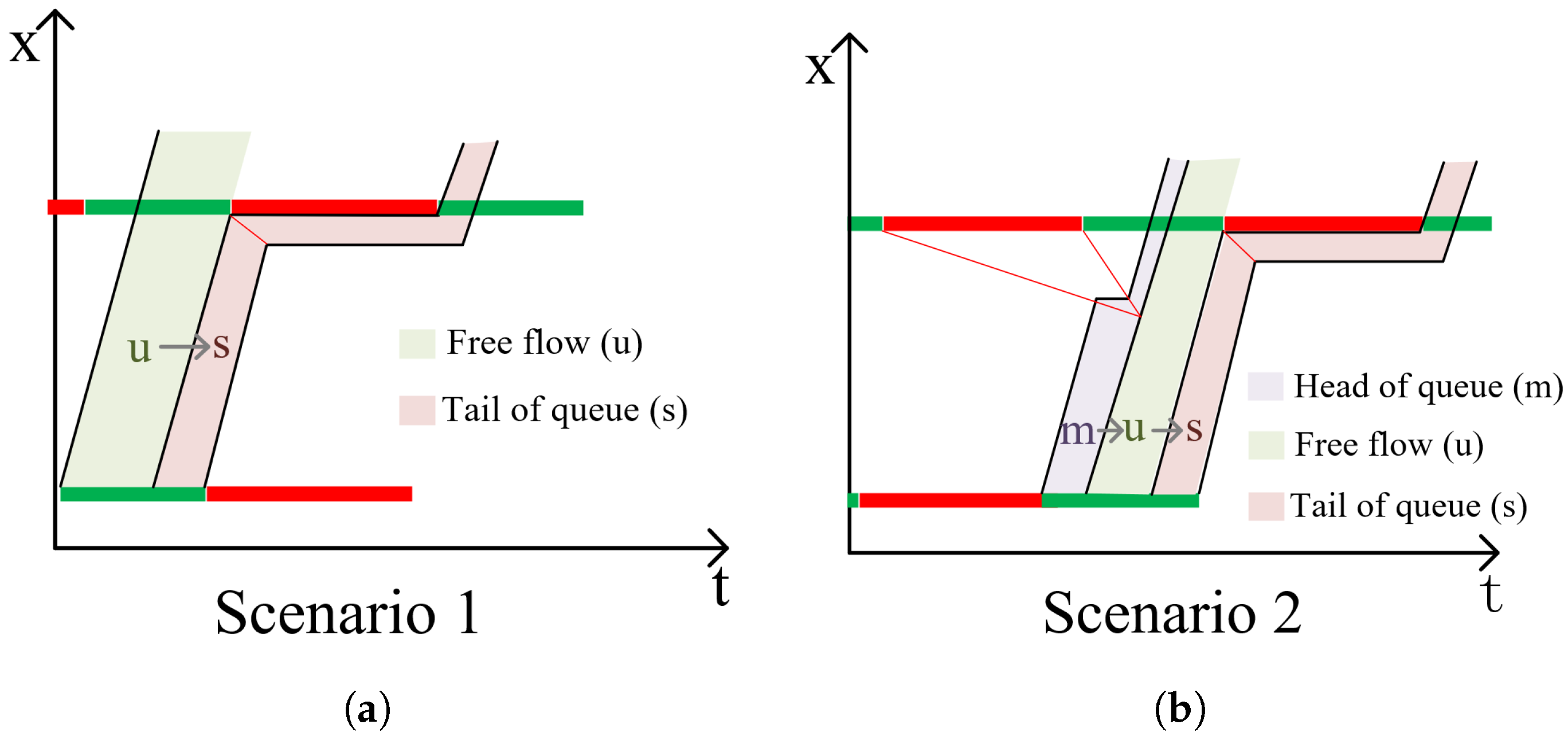
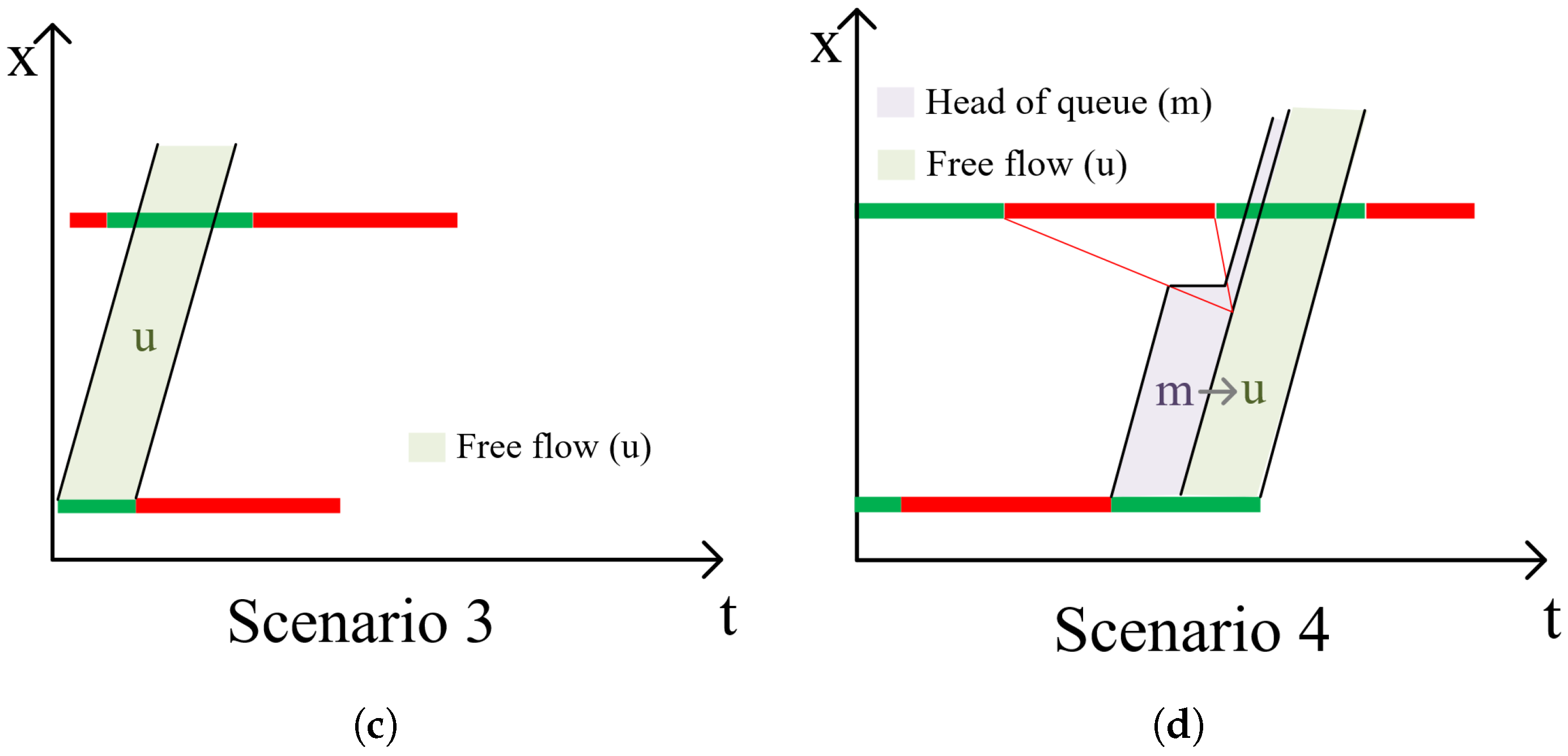
The state transitions among these three states reflect the physical process of a platoon moving through the intersection. The evolution of a platoon can be modeled as a sequence of these states. Based on the platoon’s arrival time relative to the signal phase, four typical state-transition scenarios can occur:

• Scenario 1 ($u\to s$): A group of free-flow vehicles (State u) arrives, but subsequent vehicles begin to queue due to a signal change, causing a transition to tail-of-queue delay (State s).
• Scenario 2 ($m\to u\to s$): A queue dissipates (State m), allowing a set of vehicles to pass in free-flow (State u), before a new queue begins to form near the end of the green phase (State s).
• Scenario 3 (u): An entire platoon passes through the intersection during a “green wave” or otherwise unimpeded, with all vehicles remaining in the free-flow state (State u).
• Scenario 4 ($m\to u$): A queue fully dissipates (State m), and all subsequent vehicles observed proceed in free-flow (State u) until the end of the observation window.

It is important to note that while the physical descriptions of states m and s involve dynamic trends in travel time (e.g., decreasing for a dissipating queue), the standard HMM employed in this study simplifies this by assigning an independent observation distribution to each state. The model primarily distinguishes between these different congestion states by learning the state transition probabilities and analyzing the sequence of states, rather than by directly modeling trends within the emission probabilities. For instance, the Viterbi algorithm, by finding the most likely state sequence, can effectively differentiate typical patterns such as $m\to u$ (queue dissipation) from $u\to s$ (queue formation).

The HMM’s state transition matrix $A=\left\{a_{ij}\right\}$ (where $a_{ij}=\mathrm{Pr}(S_g=j|S_{g-1}=i)$) can perfectly characterize all the above scenarios probabilistically by learning from the mixed data. These states and their corresponding transition scenarios are visually illustrated in Figure 3.

The HMM framework is illustrated in Figure 4; this layered structure explicitly models how latent congestion states (upper layer) probabilistically generate observable travel times (lower layer) while accounting for the chronological sequence of vehicles passing through downstream intersections.

The input data consists of a sequence of tuples $(\mathrm{departure}\mathrm{time},\mathrm{Travel}\mathrm{time})$ sorted chronologically. The travel time component is selected as the observation sequence $T_{1:G}=\{T_1,T_2,\dots ,T_G\}$, where $T_g$ represents the travel time of the g-th vehicle in the set. The departure time through the downstream intersection is used for temporal alignment but not directly incorporated into the HMM framework.

We model the matched travel-time sequence and its latent congestion states with a first-order HMM. The joint probability factors into an initial term, state transitions, and emissions as follows:

$$\mathrm{Pr}(T_{1:G},S_{1:G}\mid \theta )=\mathrm{Pr}\left(S_1\right)\prod _{g=2}^G\mathrm{Pr}(S_g\mid S_{g-1})\prod _{g=1}^G\mathrm{Pr}(T_g\mid S_g).$$

(1)

Notation used in Equation (1).

• $S_g\in \{m,u,s\}$: hidden state of the g-th observation (queue head m, free flow u, queue tail s).
• $T_g\in \mathbb{R}$: link travel time (s) of the g-th observation; $T_{1:G}=\{T_1,\dots ,T_G\}$ with $g=1:G$.
• ${\pi }_i=\mathrm{Pr}(S_1=i)$: initial state probabilities.
• $A= \left[a_{ij}\right]$: transition matrix with $a_{ij}=\mathrm{Pr}(S_g=j\mid S_{g-1}=i)$ and i (origin), j (destination) $\in \{m,u,s\}$.
• $B=\left\{b_i(·)\right\}$: emission family; $b_i\left(T_g\right)=\mathcal{N}(T_g\mid {\mu }_i,{\mathsf{\Sigma }}_i)$ (univariate case ${\mathsf{\Sigma }}_i={\sigma }_i^2$).
• $\theta =\{\pi ,A,B\}$: parameter set of the HMM.

A compact list of all symbols is provided in

Table 1. Notation and symbols.

Symbol	Meaning
$i,j$	Hidden states; $i,j\in \{m,u,s\}$ (queue head m, free flow u, queue tail s).
$g=1:G$	Index of matched observations in the current window.
G	Length of observation sequence $T_{1:G}$.
$S_g$	Hidden state at index g.
$T_g$	Travel time observation at index g (s).
$\pi$	Initial state probabilities $\left\{{\pi }_i\right\}$.
$A= \left[a_{ij}\right]$	Transition matrix; $a_{ij}=\mathrm{Pr}(S_g=j\mid S_{g-1}=i)$.
$B=\left\{b_i\right\}$	Emission family; $b_i\left(T_g\right)=\mathcal{N}(T_g\mid {\mu }_i,{\mathsf{\Sigma }}_i)$.
${\mu }_i,{\mathsf{\Sigma }}_i$	mean and covariance (here ${\mathsf{\Sigma }}_i={\sigma }_i^2$) of state-i emission.
L	Link length (m).
W	Rolling-window length for online re-estimation.

.

Since these parameters are not known beforehand, they must be learned directly from the observed data sequence $T_{1:G}$. For this task, we employ the Baum–Welch algorithm [29,30]. This algorithm, a specific application of the expectation-maximization (EM) procedure, iteratively adjusts the parameters $\theta =\{\pi ,A,B\}$ to maximize the likelihood of the observed travel times, as expressed in Equations (2) and (3). The detailed steps are provided in Appendix A as Algorithm A1.

$${\theta }^{*}=\underset{\theta }{\arg \max }\mathrm{Pr}\left(T_{1:G}|\theta \right)$$

(2)

$$\mathrm{Pr}\left(T_{1:G}\right|\theta )=\sum _{S_{1:G}}\mathrm{Pr}(T_{1:G},S_{1:G}|\theta ).$$

(3)

The HMM in this study uses continuous observations: each $T_g$ is a scalar link travel time and $b_i\left(T_g\right)=\mathcal{N}(T_g\mid {\mu }_i,{\sigma }_i^2)$. Only the hidden state $S_g\in \{m,u,s\}$ is discrete.

Once the model parameters $\theta$ have been estimated using the Baum–Welch algorithm, the next step is to use these parameters to infer the most probable sequence of hidden states that corresponds to the observed travel times. This process, known as decoding, is accomplished using the Viterbi algorithm.

The Viterbi algorithm [31,32] finds the single most likely state sequence ${\widehat{S}}_{1:G}$ given the observations $T_{1:G}$ and the now-trained model parameters $\theta$, as shown in Equation (4). This dynamic programming approach recursively computes the maximum likelihood path through the trellis of states, with the procedure detailed in Appendix A as Algorithm A2.

$${\widehat{S}}_{1:G}=\arg \underset{S_{1:G}}{\max }\mathrm{Pr}\left(S_{1:G}|T_{1:G},\theta \right)$$

(4)

Finally, the inferred state sequence ${\widehat{S}}_{1:G}$ is used to partition the data into three groups corresponding to states $\{s,m,u\}$. The group with the smallest mean is identified as the free-flow group (state u).

3.2.3. Free-Flow Speed Distribution Estimation

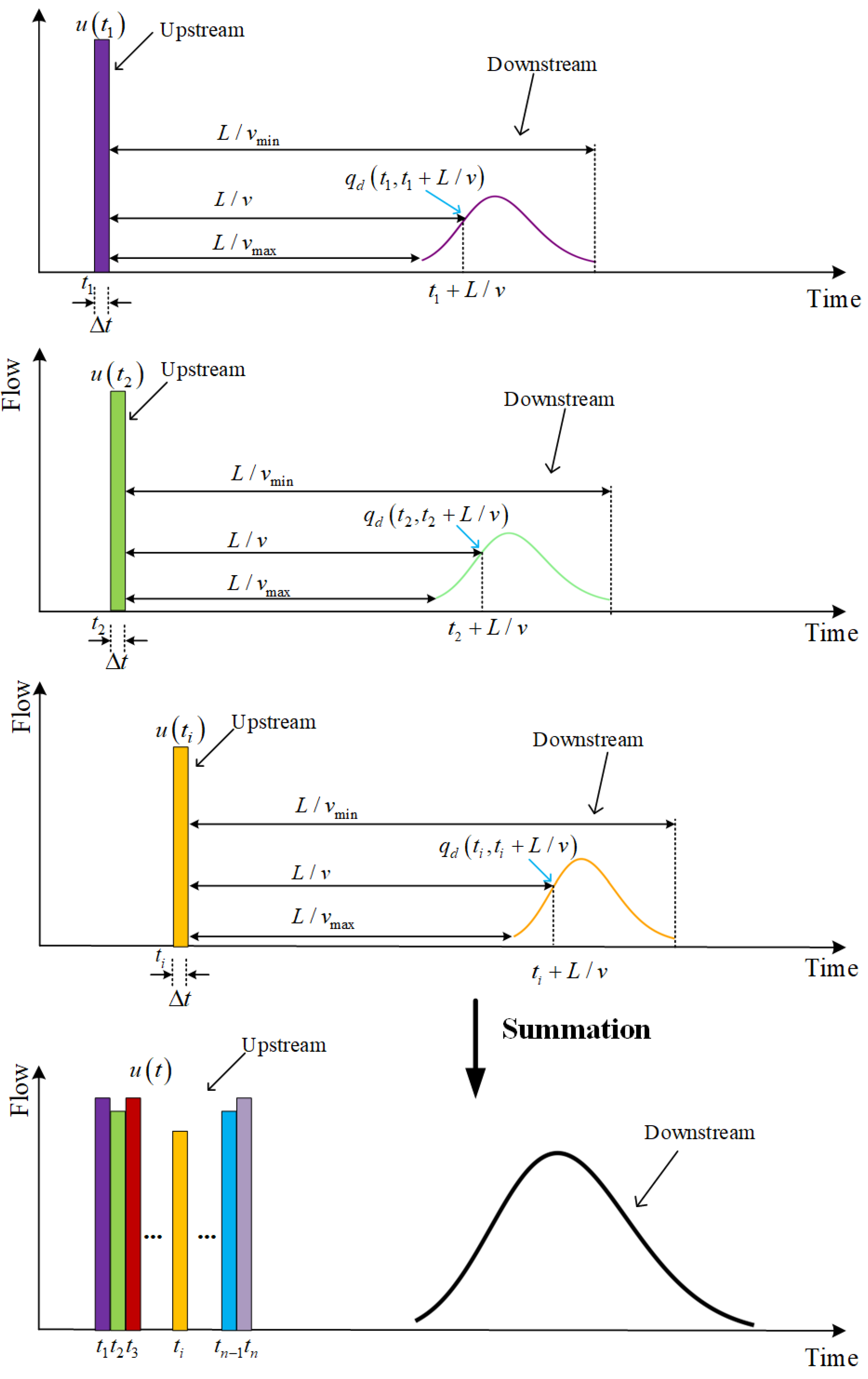
After obtaining the free-flow group, the parameters of the platoon dispersion model can be dynamically estimated. To establish the dynamic platoon dispersion model, we propose the following microscopic driving assumptions:

• Speed heterogeneity: The speeds of different vehicles within the platoon are not uniform; instead, they are independent and identically distributed (i.i.d.) random variables following a common free-flow speed distribution $f_{tu}\left(v\right)$.
• Individual speed constancy: The speed $v_i$ of any individual vehicle i is assumed to be constant throughout its journey along the link from the upstream to the downstream intersection.

In this study, the free-flow speed distribution function is assumed to follow a truncated normal distribution, as given by the following formula:

$$f_{tu}\left(v\right)={\displaystyle \frac{c}{\sqrt{2\pi }{\sigma }_{tu}}}\exp \left(-{\displaystyle \frac{{(v-{\mu }_{tu})}^2}{2{\sigma }_{tu}^2}}\right),v_{\min }\le vs.\le v_{\max }$$

(5)

where c is the coefficient of truncated distribution, ${\mu }_{tu}$ is the average speed at time $t_u$ over a 10 min time window, ${\sigma }_{tu}$ is the mean square deviation of speed at time $t_u$ over a 10 min time window, $v_{\min }$ is the minimum speed at time $t_u$ over a time 10 min window, and $v_{\max }$ is the maximum speed at time $t_u$ over a time 10 min window.

Within the free-flow group, the free-flow speed set can be obtained $V_{1:M}=\{v_1,v_2,\dots ,v_M\}$. Here M is the number of samples in the free-flow group within the current window. The parameters in Equation (5) can be estimated using the following formula:

$${\mu }_{tu}={\displaystyle \frac{1}{M}}\sum _{i=1}^M{v}_i$$

(6)

$${\sigma }_{tu}^2={\displaystyle \frac{1}{M}}\sum _{i=1}^M{(v_i-{\mu }_{tu})}^2$$

(7)

$$v_{\min }=\min \left(v_i\right),i=1,2,\dots ,M$$

(8)

$$v_{\max }=\max \left(v_i\right),i=1,2,\dots ,M$$

(9)

$$c^{-1}={\int }_{v_{\min }}^{v_{\max }}{\displaystyle \frac{1}{\sqrt{2\pi }{\sigma }_{tu}}}\exp \left. [-{\displaystyle \frac{{(v-{\mu }_{tu})}^2}{2{\sigma }_{tu}^2}}\right]dv$$

(10)

3.3. Dynamic Platoon Dispersion Model

Before detailing the prediction model, it is crucial to clarify the logical link between the parameter estimation based on a data subset and the arrival prediction for the entire traffic stream. The methodology rests on the following premises:

1.

HMM training data source: The travel time sequence $T_{1:G}$ used to train the Hidden Markov Model is constructed exclusively from vehicles successfully matched by the upstream and downstream ALPR systems. This sequence is sorted chronologically based on the vehicles’ departure times from the downstream intersection.

2.

Core generalization assumption: We posit a core assumption that the free-flow travel behavior of the successfully matched vehicles is statistically representative of the entire vehicle population on the link. This assumption is reasonable as the success of ALPR matching is generally independent of a driver’s free-flow speed choice. Consequently, the free-flow speed distribution $f_{tu}\left(v\right)$ estimated from the matched data subset is considered applicable to all vehicles.

3.

Prediction workflow: In the prediction stage, the model utilizes the complete upstream departure flow $u\left(t_u\right)$, which is directly recorded by the upstream ALPR detector and includes all vehicles, irrespective of whether they are later matched. The dynamic platoon dispersion model then applies the generalized free-flow speed distribution $f_{tu}\left(v\right)$ to this complete departure flow to calculate the dispersion of each vehicle platoon.

Having established these principles, the aggregated flow distribution of vehicles arriving at the downstream intersection can be derived. The flow departing from the upstream section at time $t_u$ and arriving at the downstream intersection at time $t_d$ is illustrated in Figure 5, with the formulation expressed as follows [22]:

1. When $L/v_{\min }\le L/v_{\max }+\Delta t$

$$\begin{array}{cc}\hfill & q_d(t_u,t_d)=\hfill \\ \hfill & \left\{\begin{array}{c}0,t_d-t_u<L/v_{\max }\mathrm{or}{t}_d-t_u>L/v_{\min }+\Delta t\hfill \\ u\left(t_u\right){\int }_{L/t_d}^{v_{\max }}{f}_{t_u}\left(v\right)dv,L/v_{\max }\le t_d-t_u<L/v_{\min }\hfill \\ u\left(t_u\right){\int }_{v_{\min }}^{v_{\max }}{f}_{t_u}\left(v\right)dv,L/v_{\min }\le t_d-t_u<L/v_{\max }+\Delta t\hfill \\ u\left(t_u\right){\int }_{v_{\min }}^{L/(t_d-\Delta t)}{f}_{t_u}\left(v\right)dv,\hfill \\ L/v_{\max }+\Delta t\le t_d-t_u<L/v_{\min }+\Delta t\hfill \end{array}\right.\hfill \end{array}$$

(11)

2. When $L/v_{\min }>L/v_{\max }+\Delta t$

$$\begin{array}{cc}\hfill & q_d(t_u,t_d)=\hfill \\ \hfill & \left\{\begin{array}{c}0,t_d-t_u<L/v_{\max }\mathrm{or}{t}_d-t_u>L/v_{\min }+\Delta t\hfill \\ u\left(t_u\right){\int }_{L/t_d}^{v_{\max }}{f}_{t_u}\left(v\right)dv,L/v_{\max }\le t_d-t_u<L/v_{\max }+\Delta t\hfill \\ u\left(t_u\right){\int }_{L/t_d}^{L/(t_d-\Delta t)}{f}_{t_u}\left(v\right)dv,\hfill \\ L/v_{\max }+\Delta t\le t_d-t_u<L/v_{\min }\hfill \\ u\left(t_u\right){\int }_{v_{\min }}^{L/(t_d-\Delta t)}{f}_{t_u}\left(v\right)dv,\hfill \\ L/v_{\min }\le t_d-t_u<L/v_{\min }+\Delta t\hfill \end{array}\right.\hfill \end{array}$$

(12)

where $q_d(t_u,t_d)$ is the flow that departs upstream at time $t_u$ and arrives downstream at time $t_d$, $u\left(t_u\right)$ is the flow that departs upstream at time $t_u$, $\Delta t$ is a unit time interval (s) and L is the link length (m).

The aggregated arriving flow distribution is computed by accumulating the arriving flows at the downstream for all upstream departing flows.

$$q_d\left(t_d\right)=\sum _{t_u=t_d-L/v_{\min }}^{t_d-L/v_{\max }}{q}_d(t_u,t_d)$$

(13)

4. Case Study

4.1. Simulation Scenario

This study is conducted entirely in simulation using the open-source road traffic simulator SUMO [33]. The run spans 2 h; the first 10 min are treated as a warm-up and excluded from evaluation. The simulated test corridor comprises two coordinated signalized intersections on Jincheng Rd: the upstream junction at Jinli Rd × Jincheng Rd and the downstream junction at Gongren Rd × Jincheng Rd (see Figure 6). The saturation flow rate is $0.5$ veh/s/lane. Both controllers operate with a common cycle of $C=100$ s. The upstream intersection uses four-phase splits of 29 s/15 s/21 s/15 s, while the downstream intersection uses 32 s/14 s/20 s/14 s. Signals are coordinated with a mainline offset of $\varphi =50$ s to generate progressing platoons from upstream to downstream. The inter-signal spacing between the two intersections is 700 m.

Within SUMO, virtual ALPR detectors are placed at the stop lines of the through approaches at both intersections. During effective green, each detector emits an anonymized plate (vehicle) ID and the timestamp at which the vehicle crosses the stop line, producing (i) the departure sequence and (ii) the matched link travel times between the two sites. To obtain an independent validation target that is not used for model calibration, we additionally place a mid-block virtual ALPR detector located 500 m downstream of the upstream stop line; its observed arrivals serve as the ground-truth reference for evaluating the accuracy of the downstream-arrival predictions propagated from the upstream intersection. These validation data are excluded from model calibration to ensure an unbiased assessment of prediction performance at this intermediate location.

The SUMO–HMM pipeline proceeds as follows. Stop-line crossing events are streamed via TraCI and logged as (vehicle ID, time, site). Upstream and downstream events are matched by ID to obtain continuous-valued link travel times $T_g=t_{\mathrm{down}}-t_{\mathrm{up}}$, which form the HMM observation sequence $T_{1:G}$. The HMM thus operates on continuous-valued observations with Gaussian emissions $b_i\left(T_g\right)=\mathcal{N}(T_g\mid {\mu }_i,{\mathsf{\Sigma }}_i)$; only the hidden states $S_g\in \{m,u,s\}$ are discrete. In parallel, upstream releases $u\left(t_u\right)$ and predicted downstream profiles $q_d\left(t_d\right)$ are time-binned with bin size B solely for platoon-dispersion propagation and evaluation—this binning does not quantize $T_g$ nor alter the continuous emission modeling. Parameter learning uses a rolling window of length W and is updated every $\Delta I$; matched pairs contribute to learning, whereas all released vehicles contribute to prediction. Lightweight Python scripts (TraCI + pandas/numpy and hmmlearn) implement event logging, ID matching, window management, and HMM training/decoding; random seeds are fixed for reproducibility. The hardware platform and software stack are summarized in

Table 2. Hardware specifications.

Component	Specification
CPU	Intel Core i7-12700
Memory	16 GB DDR5
Storage	1.5 TB NVMe SSD
GPU	NVIDIA RTX 4050 (6 GB)

and

Table 3. Software platform and libraries.

Software	Version
OS	Windows 11
Python	3.10.1
SUMO	1.23.0
Key libraries	numpy 1.26, pandas 2.2, scipy 1.13, matplotlib 3.8
HMM toolkit	hmmlearn 0.3.3

.

4.2. Experimental Protocol

This section specifies the comparison models (with final naming) and the robustness procedure used in the SUMO testbed.

For the naming convention, we use short acronyms in tables and figures and provide expanded names on first mention.

4.2.1. Models for Comparison

To evaluate overall predictive accuracy and to quantify the contribution of individual modules, we compare the following models in

Table 4. Model comparison.

ID	Model Name	HMM Filtering	Free-Flow Distribution	Dispersion Kernel	Online Update
HMM+DD	Proposed (time-varying dispersion)	✓	Online (rolling window)	Time-varying	✓
DD–NoHMM	Ablation—remove HMM	✗	Online	Time-varying	✓
SD	Ablation—freeze updates	✓	Static (initialized once)	Time-varying	✗
FK	Classical fixed-kernel baseline	✗	N/A	Static (literature constants)	✗
FTT	Fixed travel time, no dispersion	✗	N/A	None (constant offset)	✗

Notes. FTT propagates the upstream release by a constant offset equal to the median free-flow travel time estimated once on a calibration subset; no dispersion is applied. FK represents the conventional practice of using a static platoon-dispersion kernel with the literature/empirical constants and without data-driven filtering or updating. ✓ indicates the presence of a feature, whereas ✗ denotes its absence.

. All models use the same upstream release sequence, network geometry, and signal timing. For models with online updates, parameters are re-estimated every $\Delta I=1$ min using a rolling window of $W=10$ min. Evaluation uses a prediction horizon of $H=100$ s and a bin size of $B=5$ s.

4.2.2. Robustness to ALPR Matching Rate

To assess sensitivity to reduced ALPR data availability, we uniformly down-sample the set of successfully matched trips to target matching-rate levels of 90%, 75%, 60%, and 45%. For each level, we run the HMM-based free-flow identification and parameter-estimation procedure on the down-sampled ALPR dataset to obtain the estimated free-flow parameters $({\mu }_{\mathrm{est}},{\sigma }_{\mathrm{est}})$.

Reference for free-flow statistics. The true free-flow speed distribution used for parameter-error benchmarking is derived directly from SUMO vehicle trajectories: we collect link traversals that exhibit no stop-and-go (continuous motion above a small speed threshold and no queueing) and compute the reference mean and standard deviation $({\mu }_{\mathrm{true}},{\sigma }_{\mathrm{true}})$. ALPR-based estimates at each matching-rate level are then compared against $({\mu }_{\mathrm{true}},{\sigma }_{\mathrm{true}})$.

At each level, we report the deviations of the ALPR-estimated free-flow parameters from the trajectory-derived reference.

4.3. Evaluation Metrics

This section defines the metrics used to assess downstream arrival-prediction accuracy and robustness in the SUMO testbed. Unless otherwise stated, evaluation uses a prediction horizon of $H=100\mathrm{s}$ and a bin size of $B=5\mathrm{s}$.

4.3.1. Count Accuracy (Per Bin)

Given observed arrivals $y_i$ and predicted arrivals ${\widehat{y}}_i$ in bin $i=1,\dots ,K$, we report:

$$\mathrm{MAE}={\displaystyle \frac{1}{K}}\sum _{i=1}^K\left|{\widehat{y}}_i-y_i\right|$$

(14)

$$\mathrm{RMSE}=\sqrt{{\displaystyle \frac{1}{K}}\sum _{i=1}^K{({\widehat{y}}_i-y_i)}^2}$$

(15)

4.3.2. Robustness to ALPR Matching Rate

At each matching-rate level $r\in \{90\%,75\%,60\%,45\%\}$, robustness is quantified at the parameter-learning stage using the trajectory-derived free-flow reference. Let $\left(\mu \right(r),\sigma (r\left)\right)$ be the ALPR-estimated free-flow parameters at level r, and $({\mu }_{\mathrm{true}},{\sigma }_{\mathrm{true}})$ denote the trajectory-derived reference. Relative errors were reported:

$${\mathrm{RE}}_{\mu }\left(r\right)={\displaystyle \frac{|\mu \left(r\right)-{\mu }_{\mathrm{true}}|}{{\mu }_{\mathrm{true}}}}$$

(16)

$${\mathrm{RE}}_{\sigma }\left(r\right)={\displaystyle \frac{|\sigma \left(r\right)-{\sigma }_{\mathrm{true}}|}{{\sigma }_{\mathrm{true}}}}$$

(17)

Two-sample Kolmogorov–Smirnov (K–S) tests between the ALPR-estimated and trajectory-derived free-flow speed distributions are also performed, reporting the p-values and D-statistics per level.

4.4. Results and Discussion

4.4.1. Overall Prediction Accuracy Against Baselines

Table 5. Overall prediction accuracy of different models under varying $v/c$ ratios.

Model	$\mathit{v}/\mathit{c}$ = 0.95		$\mathit{v}/\mathit{c}$ = 0.70		$\mathit{v}/\mathit{c}$ = 0.45
	RMSE	MAE	RMSE	MAE	RMSE	MAE
HMM+DD	0.1482	0.1240	0.0853	0.0782	0.0614	0.0572
FK	0.2038	0.1852	0.2016	0.1680	0.1049	0.0945
FTT	0.4275	0.3886	0.3465	0.2863	0.2295	0.1765

summarizes the prediction accuracy of the proposed HMM+DD model compared with two baselines (FK and FTT) under different demand levels, expressed as the ratio of volume to capacity ($v/c$). Across all traffic conditions, HMM+DD consistently outperforms the baselines in both RMSE and MAE.

At high demand ($v/c=0.95$), the proposed method reduces RMSE by 27.3% compared with FK and by 65.3% compared with FTT, while MAE is lowered by 33.1% and 68.1%, respectively. Under medium demand ($v/c=0.70$), the improvements are even more pronounced: RMSE is reduced by 57.7% relative to FK and 75.4% relative to FTT, with MAE reduced by 53.5% and 72.7%. At low demand ($v/c=0.45$), prediction errors are overall smaller, but HMM+DD still maintains superior accuracy, lowering RMSE by 41.4% compared with FK and 73.2% compared with FTT, while MAE is reduced by 39.5% and 67.6%.

These results demonstrate that the dynamic, HMM-filtered dispersion model adapts effectively to varying traffic demand levels and consistently yields more reliable predictions than static dispersion kernels or fixed-travel-time assumptions. Importantly, the advantage of HMM+DD is not limited to congested scenarios but is evident across the full spectrum of $v/c$ conditions, confirming its robustness and general applicability for real-time traffic signal control.

4.4.2. Ablation Study on HMM Filtering and Online Updates

Table 6. Ablation study on HMM filtering and online updates under varying $v/c$ ratios.

Model	$\mathit{v}/\mathit{c}$ = 0.95		$\mathit{v}/\mathit{c}$ = 0.70		$\mathit{v}/\mathit{c}$ = 0.45
	RMSE	MAE	RMSE	MAE	RMSE	MAE
HMM+DD (Proposed)	0.1482	0.1240	0.0853	0.0782	0.0614	0.0572
DD–NoHMM (w/o HMM)	0.6270	0.4898	0.3990	0.3093	0.3240	0.2492
SD (frozen updates)	0.1587	0.1417	0.1282	0.1155	0.0810	0.0675

presents the results of ablation experiments designed to isolate the effects of HMM-based free-flow filtering and online parameter updates. The comparison highlights two degraded variants of the proposed model: (i) DD–NoHMM, which removes the HMM classification and directly estimates dispersion from unfiltered travel times, and (ii) SD, which freezes parameter updates after an initial calibration.

The results show that removing HMM filtering leads to dramatic performance degradation. For example, at $v/c=0.95$, RMSE rises from 0.1482 (HMM+DD) to 0.6270 (DD–NoHMM), an increase of 323.1%, while MAE more than triples. This indicates that unfiltered travel times introduce substantial noise from queue-induced delays, severely distorting the estimated dispersion parameters. The negative impact remains evident at lower demand levels ($v/c=0.70$ and $0.45$), where errors remain 3–5 times higher than the full model.

Freezing updates (SD) results in only moderate degradation compared with HMM+DD. While errors are slightly higher across all demand levels, the relative increase is limited (e.g., RMSE grows by only 7.1% at $v/c=0.95$). This suggests that while online updates improve adaptability to changing traffic conditions, the HMM filtering plays a more decisive role in maintaining prediction accuracy.

In summary, the ablation study confirms that both HMM filtering and online updates contribute to the accuracy of the proposed model, but the filtering mechanism is the dominant factor in reducing noise and ensuring robust performance across varying traffic demand.

4.4.3. Robustness to ALPR Matching Rate

To assess the model’s sensitivity to data availability, we conducted a Monte Carlo simulation by randomly removing a certain percentage of successfully matched vehicle trips, creating scenarios with reduced ALPR matching rates. We tested the HMM-based free-flow parameter estimation at matching rates of 90%, 75%, 60%, and 45%, with 30 simulation runs for each level. The estimated free-flow parameters $({\mu }_{est},{\sigma }_{est})$ at each level were compared against a ground-truth reference derived from the underlying SUMO simulation trajectories.

Figure 7 illustrates the stability of the estimation process. The distributions of the Kolmogorov–Smirnov D-statistic, its corresponding p-value, and the relative errors in the mean ($R{E}_{\mu }$) and standard deviation ($R{E}_{\sigma }$) of the free-flow speed are presented. Across all tested matching rates, the relative errors for the mean free-flow speed ($R{E}_{\mu }$) remain consistently low, with median values well below 2%. Similarly, the relative errors for the standard deviation ($R{E}_{\sigma }$) are contained, staying below 7% even at the lowest matching rate of 45%. The K-S D-statistics are small, and the p-values are generally well above the 0.05 significance threshold, indicating no statistically significant difference between the estimated and true free-flow distributions.

Table 7. Summary of Monte Carlo robustness simulation results (N = 30 runs/level).

Metric	r = 45%	r = 60%	r = 75%	r = 90%
Mean $R{E}_{\mu }$ (%)	1.29	1.59	1.41	1.28
Std Dev $R{E}_{\mu }$ (%)	0.57	1.66	0.37	0.19
Mean $R{E}_{\sigma }$ (%)	5.82	6.23	5.07	4.54
Std Dev $R{E}_{\sigma }$ (%)	3.43	5.07	2.75	2.40
Mean K-S D-statistic	0.088	0.096	0.080	0.071
Mean K-S p-value	0.419	0.369	0.305	0.351

summarizes the numerical results, reinforcing the visual findings from the boxplots. The mean relative errors for both $\mu$ and $\sigma$ show remarkable stability and do not exhibit a strong degradation trend as the matching rate decreases. This suggests that the HMM framework can reliably estimate free-flow speed parameters even with substantial data loss, a critical feature for real-world ALPR systems where matching rates can vary. The model’s performance is robust, ensuring that the foundational parameters for downstream traffic applications remain accurate across a wide range of data-quality scenarios.

4.4.4. Limitations and Alternatives

The Viterbi decoder yields a single most-probable state path under a fixed parameter set $\theta =\{\pi ,A,B\}$ within each update cycle. This implies local stationarity for transitions/emissions and hard assignments that may under-represent posterior uncertainty near boundaries. In traffic dynamics, these assumptions can be challenged by phase-dependent non-stationarities (e.g., offset shifts, demand surges).

This issue is mitigated in our framework through frequent rolling re-estimation ($W=10$ min, update every $\Delta I=1$ min) to refresh $\{\pi ,A,B\}$ from the latest window while keeping decoding lightweight for real-time use.

When stronger non-stationarity is expected, alternative formulations may be considered, one may use posterior decoding (per-sample MAP), non-stationary or hierarchical HMMs (time-varying $A,B$), hidden semi-Markov models (dwell times), or switching state-space models/particle filters to capture regime changes. These extensions can plug into our ALPR pipeline at a higher computational cost.

5. Conclusions

This work addressed the gap between point-based ALPR observations and the predictive, link-level arrival profiles required for modern urban signal control. We presented a HMM-filtered dynamic platoon-dispersion framework that converts sparse license plate timestamps into real-time downstream arrival predictions. The approach operates with existing roadside infrastructure and requires neither CV penetration nor continuous trajectories.

Across a corridor-scale simulation study, the proposed method consistently outperformed fixed-kernel and fixed-travel-time baselines over a wide demand range. Ablation analyses showed that the HMM-based filtering is the primary source of accuracy gains by isolating free-flow samples from signal-induced delays, while online dispersion updates add adaptability under time-varying conditions. Robustness tests further indicated stable parameter estimates under low ALPR matching rates, supporting deployability when data quality fluctuates.

This framework offers strong practical relevance, given that it is lightweight and depends solely on already deployed ALPR cameras, the predicted arrival profiles $q_d\left(t_d\right)$ can be fed directly to adaptive signal strategies (e.g., split/offset updates, spillback mitigation, and progression maintenance) on rolling horizons, enabling near-term integration into existing traffic management centers.

The framework has several limitations and corresponding future directions. HMMs assume a fixed number of predefined states and locally stationary transitions/emissions within each update cycle, and Viterbi provides a single-path decoding; we mitigate these effects via frequent rolling re-estimation. Data-wise, ALPR does not provide continuous ground-truth arrival flows, which limits the direct use of fully supervised deep predictors (e.g., LSTM/Transformer). Our design explicitly targets this constraint by exploiting discrete ALPR events via HMM filtering and dispersion; when richer labels become available, hybrid pipelines that wrap the dispersion stage with learning-based predictors merit investigation. Promising model extensions include non-stationary or hierarchical HMMs, hidden semi-Markov models (explicit dwell times), and switching state-space models to capture regime changes, as well as fusion with complementary sensors (e.g., roadside radar or CV probes). We also plan field tests on operational corridors to assess end-to-end impacts on signal performance.