A Deep Multi-Task Learning Model for OD Traffic Flow Prediction Between Highway Stations

Abstract

The rapid development of highways greatly affects the flow of people, finance, goods, and information between cities, and monitoring the OD flow of travel has become a very important task for intelligent transportation systems (ITS). The temporal dynamics and complex spatial correlations of OD traffic distribution, as well as the sparsity and incompleteness of data caused by uneven traffic distribution, make OD traffic prediction complex and challenging. This paper proposes a multi-task prediction model for OD traffic between highway stations. The model adopts a hard parameter shared multi-task learning network structure, which is divided into sub-task learning inflow trend modules, sub-task learning outflow trend modules, and main task learning modules for OD traffic. At the same time, the attraction intensity matrix between stations is constructed using the population density data as the external feature of the sub-task module for outlet outflow flow, and stronger constraints between tasks are introduced to achieve better fitting results. Finally, an OD flow prediction case experiment was conducted between stations on highways in Sichuan Province. The experimental results showed that the proposed model not only had higher accuracy in predicting results than other baseline models, but also had better effectiveness and robustness.

1. Introduction

In recent years, there has been a significant expansion and enhancement of the highway network. Highways, serving as the primary backbone of this network, play a crucial role in effectively interlinking various transportation modes. The rapid development of highways has greatly improved the transportation efficiency of the transportation system and the travel efficiency of residents, promoting economic connections and resource flow between regions. Refinement and intelligent management and control of highways, encompassing congestion management, accident response, safety rescue, and toll optimization, have emerged as paramount and pressing concerns for the advancement of highways in the contemporary era. Predicting highway flow stands as a foundational step in addressing these challenges, especially forecasting the OD flow of travel has emerged as a critical task [1].

The evolution of information technology and the proliferation of intelligent transportation systems have enabled dynamic data acquisition for highways. Consequently, there is an imperative need to address the theoretical task of formulating predictive models based on such dynamic data. As of now, the installation rate of ETC for automobiles in various provinces (regions, cities) has reached over 80%, and the utilization rate of ETC for vehicles passing through highways has reached over 90%. The electronic toll collection system utilizes vehicle automatic recognition technology to complete wireless data communication between vehicles and toll stations, enabling automatic vehicle recognition and exchange of relevant toll data. It can also record sea volume transaction data, including entrance and exit ramps, time, vehicle type, driving direction, license plate number, etc. How to effectively and quickly utilize this information, analyze historical data for data statistics and internal connection mining, apply it to predict traffic flow, optimize road network design, allocate resources reasonably, reduce congestion, deeply mine the traffic characteristics it presents, and effectively apply them to the operation analysis of highways has become the most concerned issue for operators and researchers.

The OD matrix sequence under investigation is a three-dimensional tensor, encapsulating intricate temporal and spatial correlation data. This presents substantial challenges for associated research. Particularly, when examining OD matrix true value sequences across various historical periods, researchers must discern the spatial correlations among traffic nodes and the temporal correlations among sequence position vectors. Subsequently, these findings are amalgamated to predict OD matrix values for one or more forthcoming periods, serving as the target output. The current study seeks to understand the mutual information between graph nodes by embedding each traffic node and its associated feature vector into the graph structure. This process heavily relies on the establishment of the graph structure itself. However, topological graph structures are often built upon pre-established prior information such as inter-node distance [2], connectivity [3], and adjacency [4]. Consequently, this hinders the graph learning process in capturing the inherent dependency relationships between nodes that lack edge connections. Nevertheless, certain studies depend on attention learning or convolutional networks for correlation learning among nodes across the entire domain. However, this approach overlooks the intrinsic spatial positional relationships present in traffic data. Current research methodologies are unable to equitably manage the intrinsic and extrinsic relationships among transportation nodes.

In this paper, we propose a multi-task prediction model for OD traffic flow between highway stations considering the influence of population factors. By studying the prediction of OD traffic flow, the population flow patterns between different ODs can be predicted, revealing the impact of population factors on cross regional traffic OD distribution, and providing data support for intelligent management and control of highways [5]. The model adopts a hard parameter shared multi-task learning network structure, which is divided into sub-task learning modules for inflow trend learner, sub-task learning modules for outflow trend learner, and main task learning module for OD traffic flow prediction. At the same time, we use population density data from yearbooks to construct an attraction intensity matrix between stations as the external feature of the sub-task module for outflow trend learner, and introduce stronger constraints between tasks to achieve better fitting results. Finally, an OD traffic flow prediction case experiment was conducted between stations on highways in Sichuan Province to evaluate and analyze the performance of the proposed model. The experimental results showed that the proposed model not only had higher accuracy in predicting results than other baseline models, but also had better effectiveness and robustness.

Our main contributions are listed as follows:

• We will design a hybrid deep learning model with a multi-task learning framework for OD traffic prediction.
• We innovatively considered the impact of population factors in the prediction algorithm.
• We evaluated the performance of the proposed framework using actual traffic flow data. The results demonstrated the advantages of our framework compared to the four baseline methods.

2. Related Studies

Generally, OD traffic flow prediction aims to predict the traffic flow at each starting and ending point. The research on OD matrix prediction can be divided into three stages: the first stage is mainly based on statistical learning methods to model the temporal trend of OD matrix. The second stage of research is mainly based on the algorithms of recurrent neural networks, convolutional neural networks, and attention mechanisms, and has made breakthrough progress in mining temporal and spatial mutual information. After 2017, graph neural networks, especially graph convolutional networks, have become the mainstream of spatiotemporal relationship learning research and have been widely used in traffic related problems, bringing OD matrix prediction problems into a new stage of graph learning. This section will introduce the current research status of OD matrix prediction problem at home and abroad from three parts: traditional research methods, research based on deep learning algorithms, and research based on graph neural networks.

Traditional prediction methods can be roughly divided into two categories: growth coefficient method and comprehensive method [6]. The growth coefficient method assumes that the future OD distribution will be the same as the existing OD distribution, and based on this assumption, predicts the future OD, mainly including the constant growth coefficient method, the average growth coefficient method, the Dett method, and the Follett method [7]. Li Xiamiao et al. cleverly adopted the gravity model method, utilizing more easily obtainable population Using GDP and other data resources to infer the OD traffic matrix, and then predict the passenger flow between stations [8]. Li et al. treated OD matrix prediction as a non-negative matrix factorization problem and used autoregressive models to process the decomposition results to obtain the prediction target [9]. This method does not involve changes in traffic impedance, and once there are significant changes in land use and economic structure, this method will not be applicable [10]. The comprehensive method starts from the actual OD traffic volume, assumes human travel behavior based on the distribution pattern of actual OD, analyzes the distribution pattern of OD matrix, constructs a model, calibrates model parameters, and predicts future OD [11]. Mahev et al. [12] proposed using Bayesian estimation to predict OD matrices. CaScetta et al. [13] applied the generalized least squares method to the inverse derivation of OD matrices. H. Spiess et al. [14] proposed using a maximum likelihood estimation model to estimate the OD matrix. Fisk et al. [15] proposed combining the maximum entropy method with the user optimal allocation model to estimate the OD matrix. Toledo et al. [16] proposed an estimation method for OD matrix using linear approximation of allocation matrix, where the allocation ratio is linearly correlated with travel demand. SR Hu et al. [17] proposed an integrated heterogeneous sensor deployment model that does not require prior OD information and path selection probability. The results show that only possible and reasonable ODs can be extracted, and the solution is not unique. Y Ji et al. [18] proposed a widely used iterative proportional fitting (IPF) method, which can solve problems without updating prior information on a large amount of on/off vehicle data. Furthermore, regardless of the given initialization matrix, it can converge to the same estimated value in the shortest computation time. J Guo et al. [19] proposed a genetic algorithm for solving the optimization model of OD matrix extraction based on the least squares model, and verified it with practical data in Nanjing, China. The results showed that the proposed method can effectively derive accurate dynamic OD matrix.

Moreover, predicting OD matrices based on mathematical statistical methods has drawbacks such as high computational complexity and difficulty in deeply exploring the internal relationships of data. Therefore, the focus of subsequent research is gradually shifting towards machine learning and neural network algorithms. Yang Xiaoguang et al. [20]. used traditional BP neural networks to predict future OD matrices in 2004, pioneering the use of deep learning to study OD matrices in China. Chen et al. [21] used an improved fully connected neural network to input past OD matrix sequences and output predicted traffic flow values for the highway network during a certain period in the future.

The evolution of big data necessitates the holistic utilization of existing transportation big data for modeling and problem-solving, with the aim of enhancing the precision of prediction outcomes. Recently, the shortcomings of traditional research methodologies, namely their slow computational speed and inadequate depth of information mining, which fail to meet the real-time and accuracy demands of prediction, have led to an increasing reliance on deep learning-based methods. These methods are now predominantly used to address prediction challenges stemming from OD. Among the most noteworthy are recurrent neural networks (RNNs), convolutional neural networks (CNNs), and attention mechanisms. Considering the distinct benefits of RNNs and CNNs in managing sequential and spatial relationships, prior research has frequently combined these methods within a unified model to address the OD matrix prediction problem. Yu et al. [22] developed a hybrid model, known as SRCN, that integrates deep convolutional networks with long short-term memory networks (LSTM) to forecast a range of traffic data, including OD matrices. This process involves transforming the OD matrix, traffic flow, average speed, and other sequences within the transportation network into a series of static images. The model then employs convolutional networks to capture spatial dependencies, while utilizing LSTM to learn temporal dependencies. The learning results from these two processes are subsequently fused together for accurate prediction. Chu et al. [23] proposed a deep learning model known as Multi Scale ConvLSTM, designed to learn spatial correlations across multiple regional scales. This model incorporates two-dimensional convolution kernels of varying sizes within the convolution operation component of the ConvLong Short Term Memory Network (ConvLSTM). This feature enables the extraction of spatial correlations among nodes in diverse regions. Furthermore, the model leverages the LSTM component to unearth temporal correlation data, ultimately yielding short-term prediction values of the OD matrix. Liu [24] proposed a scenario based spatiotemporal network (CSTN), which consists of three modules. Firstly, CNN is used to extract local spatial features of the starting and ending points, and then input them into ConvLSTM for demand time evolution analysis. Finally, in order to capture the correlation between distant regions, GCC module is used to extract global correlation features.

In order to delve into the intricate temporal and spatial correlations within data, several studies have incorporated attention mechanisms. These are designed to compute the correlation weights between any node and any time period on a comprehensive global scale. Yao et al. [25] proposed an enhanced attention mechanism, building upon the traditional LSTM framework, to assess the influence of various dates and time periods on the forecasted target time period. They quantified this influence as attention weights, which were subsequently used to weight the OD matrix prediction values. In the study of graph neural networks, the adjacency relationships between nodes in the graph are represented by edges, which facilitates the transfer of feature information between nodes. Due to the high degree of fit between graph structures and transportation networks, graph neural networks are increasingly considered the primary choice for OD traffic prediction. Edges between nodes can be delineated based on diverse spatial relationships, including distance, traffic flow, and road connectivity. Through sophisticated algorithms such as graph convolution and graph attention, traffic flow data between nodes is disseminated, culminating in the computation of the OD target prediction value. Zhao et al. [26] introduced a Time Convolutional Network (T-GCN) model that has emerged as a prototype for addressing OD matrix prediction challenges. This innovative model synergistically integrates Graph Convolutional Networks (GCNs) and Gated Recurrent Units (GRUs). The GCN component is adept at learning intricate node topologies, thereby capturing spatial dependencies, while the GRU segment is proficient in discerning dynamic trends within OD data sequences, ensuring the capture of temporal dependencies. Wang [27] proposed a multi-task learning model based on grid embedding, which embeds GCN into each grid to simulate the flow transfer relationship between different grids. Ke [28] proposed a spatiotemporal residual encoding decoding multi graph convolution model, which takes OD pairs as nodes, models the non-Euclidean spatial and semantic correlations between different OD pairs, forms a multi graph adjacency matrix, and inputs it into the residual multi graph convolution model, achieving good prediction results. Chen [29] proposed a hybrid spatiotemporal network (HSTN) based on Graph Convolutional Network (GCN), attention mechanism, and Seq2Seq model to solve the problem of spatiotemporal correlation in predicting the OD matrix of ride hailing services. HSTN consists of two components, including Hybrid Space Module (HSM) and Hybrid Time Module (HTM). Zhang et al. [30] introduced a dynamic node edge attention network (DNEAT) to address the origin-destination (OD) matrix prediction issue by leveraging dynamic graph learning, considering demand generation and attraction. They incorporated a novel k-hop temporal node edge attention layer in DNEAT to capture the temporal evolution of node topology within dynamic OD graphs. Notably, the topology and corresponding weights between nodes are not predetermined as in previous studies; instead, they are learned through attention mechanisms based on distance relationships. This approach imbues the model with enhanced robustness, especially with highly sparse OD matrix data.

3. Preliminaries and Problem Definitions

3.1. Basic Concepts

The OD traffic flow between highway stations is the traffic demand from the entrance toll station to the exit toll station, express the OD traffic of all toll stations in the highway network through a matrix as follows:

$$X^t=\left(\begin{array}{ccc}{x}_{1,1}^t& \cdots & x_{1,n}^t\\ ⋮& \cdots & ⋮\\ x_{n,1}^t& \cdots & x_{n,n}^t\end{array}\right)\in {\mathit{ℝ}}^{N\times N}$$

(1)

The entrance inflow of a highway station $x^t{}_{i:}$ is defined as all traffic flow from the origin toll station $s^o=s_i$ during the t time step.

The exit outflow of highway stations $x^t{}_{:j}$ is defined as all traffic flow at the destination toll station $s^d=s_j$ during the t time step.

So for each $x^t=(x^t{}_{i:},x^t{}_{:j},x^t{}_{ij})$.

The OD traffic flow prediction between highway stations is based on historical OD data and external factors, mining hidden spatio-temporal features to establish a model, and predicting the OD of the current road network at the next time step.

$$X^t=f(X^{t-h},\cdots ,X^{t-2},X^{t-1}){\rm E}$$

(2)

where $f(\cdot )$ is a predictive function that needs to be fitted,

$t-h$ is the time step of historical data,

${\rm E}$ is an external environmental factor variable, and this study involves weather and radiation population factors.

3.2. Impact of Spatial and Temporal Factors on Traffic Data

Highway traffic flow is characterized by intricate spatiotemporal correlations, reflecting diverse and dynamic patterns that evolve in both time and space. These patterns are not only shaped by temporal and spatial dimensions but also by external environmental factors such as holidays, weather conditions, and population dynamics.

In terms of temporal characteristics of traffic data: Traffic flow data from highways demonstrate non-linear correlations in their temporal characteristics. These include adjacent time features, trend time features, and cycle time features. In short, the periodicity of time, day, and week. From Figure 1, it can be seen that the daily flow trend of the same station shows obvious morning and evening peak characteristics, and the traffic flow sequence between days shows certain periodicity and similarity, with different weekdays and weekends.

In terms of spatial characteristics of traffic data: The spatial correlation of highway traffic flow data can be bifurcated into static and dynamic spatial features. Static spatial features are characterized by geographic interdependence and pattern similarity, while dynamic spatial features are influenced by the trends in traffic flow at key original stations and the trends at key destination stations. From Figure 2, the traffic flow of node $v_3$ is not only affected by the traffic flow of neighboring nodes $v_1,v_2,v_4,\dots ,v_n$ at the current time t, and the influence coefficient can be represented by the covariance matrix, but also by the flow of traffic from node $v_i(i\ne 2)$ to node $v_2$ at time t − 1. The degree of influence is represented by a probability matrix.

In terms of external characteristics of traffic data: Firstly, the multi-source fusion processing of weather data and traffic flow at a toll station on the highway revealed that weather can affect people’s travel choices, and the changes in traffic flow vary depending on different weather types, show in Figure 3.

Secondly, the traffic flow on highways is not only affected by weather, but also has a certain correlation with holidays, as shown in Figure 4. Whether it is a holiday has a significant impact on the changes in traffic flow.

Finally, highways have strong externalities, and the distribution of traffic objectively reflects the laws of human movement. Exploring the correlation between the traffic flow of highways and their radiation population. Specifically, it examines the Origin–Destination (OD) traffic flow and radiation population data from Chengdu city in 2018. These figures are subsequently analyzed for correlation and normalized, as presented in

Table 1. Normalization of Radiation Population and OD Flow in Chengdu City.

District	Origin	Destination	Radiation Population	District	Origin	Destination	Radiation Population
Chenghua	0.07	0.26	0.43	Pujiang	0.00	0.09	0.00
Chongzhou	0.26	0.24	0.25	Qingbaijiang	0.06	0.46	0.10
Dayi	0.04	0.29	0.16	Qingyang	0.25	0.22	0.36
Dujiangyan	0.23	1.00	0.27	Qionglai	0.18	0.10	0.22
Jianyang	0.10	0.07	0.50	Shuangliu	1.00	0.06	0.75
Jinniu	0.18	0.72	0.59	Wenjiang	0.30	0.04	0.16
Jintang	0.07	0.18	0.28	Wuhou	0.68	0.07	1.00
Jinjiang	0.11	0.63	0.28	Xindu	0.52	0.00	0.40
Longquanyi	0.47	0.50	0.41	Xinjin	0.05	0.07	0.04
pengzhou	0.07	0.17	0.32	Pidu	0.74	0.05	0.37

. Pearson correlation coefficient is used for correlation measurement. It was found that the destination of highways is significantly correlated with the radiation population, as shown in Figure 5.

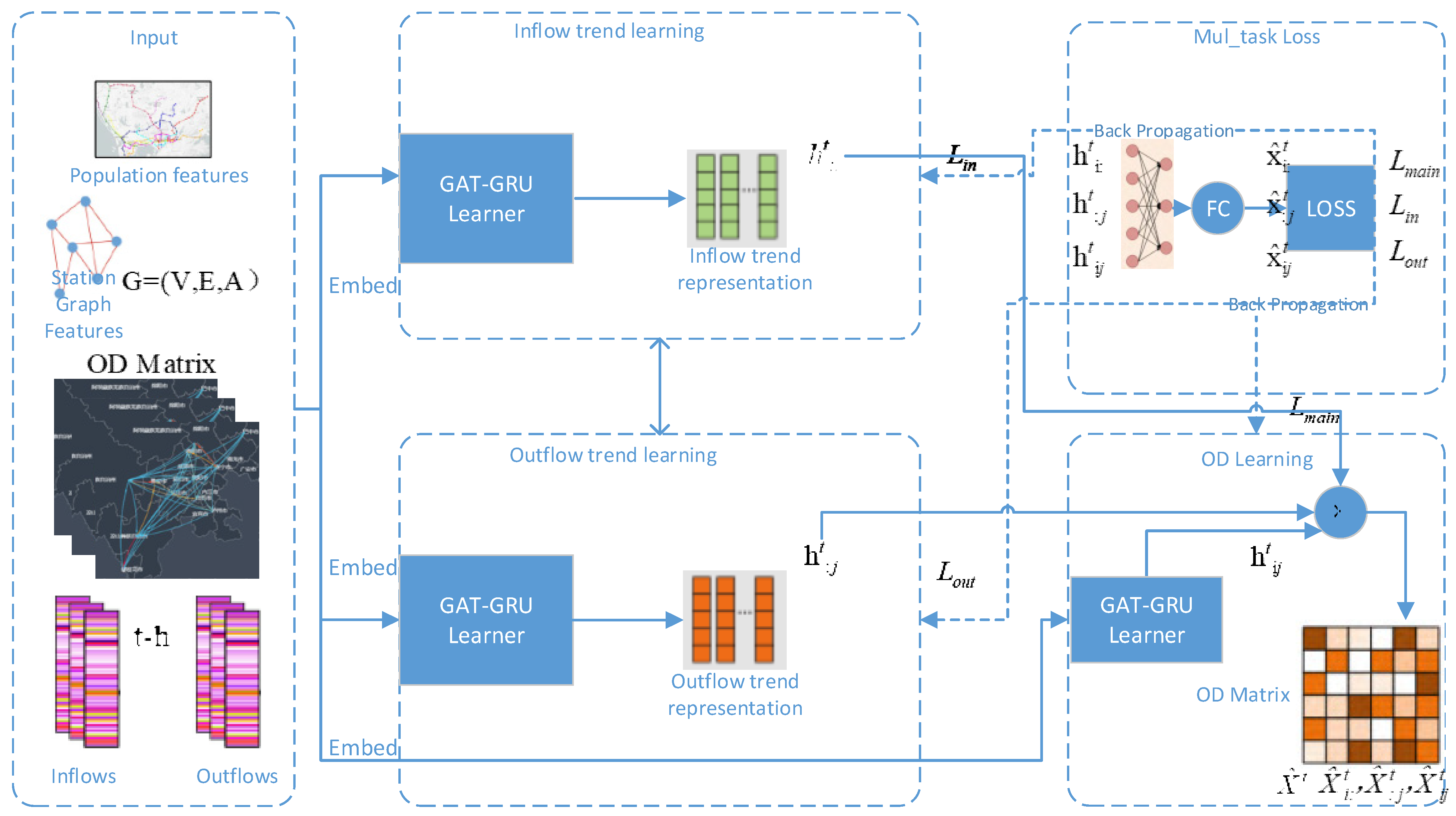
4. Model Construction

Given the temporal dynamics and complex spatial correlations of OD distribution, as well as the sparsity and incompleteness of data caused by uneven flow distribution, and the susceptibility to external factors, and the coupling effect between the population radiated by the highway network and the highway flow, this section establishes a multi-task prediction model for OD flow in the highway network considering population factors (OD_MLP). The model adopts a hard parameter shared multi-task learning network structure, which is divided into sub-task learning modules for inlet inflow flow, sub-task learning modules for outlet outflow flow, and main task learning module for OD flow. Treating the highway toll station as a cross-sectional node, the historical traffic flow of the node is processed into OD matrix, entrance inflow matrix, and exit outflow matrix using networked toll data. The static features of the graph structure of the road network toll station are constructed, combined with external weather data and population data as inputs. The internal structure of each module is composed of heterogeneous neural networks combining GAT and GRU to capture the spatiotemporal patterns of the input data. At the same time, a multi-task learning framework is used to introduce stronger constraints and obtain effective embedding representations of each subtask module, thereby improving the accuracy of OD traffic prediction between stations. The model structure is shown in Figure 6. The key symbols used in the model are defined in

Table 2. Summary of key symbols.

Symbol	Definition
$x_{i:}^t$	The traffic flow of origin Station $s_i$ during the time interval t
$x_{:j}^t$	The traffic flow of destination Station $s_j$ during the time interval t
$x_{ij}^t$	OD traffic flow between $s_i$, $s_j$ station within time interval t
$\mathrm{p}(i\to j)$	The attraction strength of the destination station $s_j$ to the origin station $s_i$
${\mathrm{h}}^t{}_{\mathrm{i}:},{\mathrm{h}}^t{}_{:j},h_{\mathrm{i}j}^t$	Hidden layer output
$L_{main},L_{in},L_{out}$	Loss functions for each subtask $s_j$
${\widehat{X}}^t$	Final model output data

.

For OD traffic prediction, assuming N toll stations are given, there are N * N OD pairs that need to be predicted at a unit time step. However, the bidirectional relationship between OD pairs requires different learning to represent and dynamically changes over time. In addition, the number of non-zero elements in the OD matrix will be much smaller than the number of zero elements, as shown in the contour map of OD for time slice in Figure 7. The horizontal axis represents exstation, the vertical axis represents enstation. The number of non-zero elements only accounts for 5.22% of the elements in the OD matrix. The high sparsity of the OD matrix makes the sensitivity and prediction accuracy of the prediction model to noise unsatisfactory. In order to better capture time-varying and bidirectional spatial relationships during the modeling process, this chapter introduces subtasks of the entrance inflow learning module and the exit outflow learning module to improve the accuracy of the main task learning module for OD traffic.

4.1. Inflow Trend Learner

The tasks of the entrance inflow learning module include learning the time-varying trend of the total amount of entrance inflow (including time, day, and week), learning the spatial interaction patterns of destination stations (spatiotemporal fusion), and learning changes influenced by external environment. The internal structure of the learning module is shown in Figure 8.

Firstly, construct a traffic map matrix ${\mathrm{G}}_{in}^t=(\mathrm{V},\mathrm{E},\mathrm{A},\mathrm{w})$.

Where $\mathrm{w}$ is representing the destination weight matrix $w_{i,j}^t={\displaystyle \frac{x_{ij}^t}{x_{i:}^t}}$.

Then, using node2vec encoding, the constructed graph structure data are random_walk to obtain spatial information encoding, and the spatial expression of historical inflow traffic data are obtained (Algorithms 1 and 2).

$$x_{i:}^s=node2vec(G)$$

(3)

$$Node\_sequence=Random\_walk(G)$$

(4)

$$x_{i:}^s=SkipGram(Node\_sequence)$$

(5)

Algorithm 1. $node2vec$ algorithm

Firstly, generate parameters related to the random walk strategy $\pi =(G,p,q)$ $G^{\prime }=(V,E,\pi )$, start node: $\mathrm{u}$, Sequence length: $l$, Generate an initialization walk sequence: $N(u)$, Number of iterations for wandering: $\mathrm{iter}=\mathrm{r}$ for $iter=1:r$  for walk_iter = 1: $l$   curr = walk[−1];   Retrieve neighbor node information of the current node $V_{curr}=GetNeihbors(curr,G^{\prime })$   Sampling based on walk strategy $s=AliasSample(V_{curr},\pi )$   Find the next node, add $s$ to $walk(u)$   Return $walk(u)$  $f=SkipGram(k,d,walk)$// Call SkipHram algorithm Return $f$

Algorithm 2. $SkipGram$ algorithm

for each node $v_i$ belonging to the current random walk sequence $N_R(u)[j-w:j+w]$   for traverse every node in the surrounding window $\omega$ of the node ${\mathrm{u}}_{\mathrm{k}}\in N_{v_i}(u)[j-w:j+w]$    Calculate loss function $\mathrm{J}(\mathsf{\Phi })=-\log {\mathrm{p}(\mathrm{u}}_{\mathrm{k}}|\mathsf{\Phi }(v_j)$    Gradient descent updates embedding matrix $\mathsf{\Phi }=\mathsf{\Phi }-\alpha \ast {\displaystyle \frac{\partial J}{\partial \mathsf{\Phi }}}$

4.  End for

5. End for

Based on the expression of historical traffic feature vectors, the GAT network was used to learn the trend of all traffic from origin station $s^o=s_i$ entering the highway and the trend learning towards the destination station $s^d=s_j$, and then can obtain dynamic spatial attention of entrance station ${\mathrm{a}}_{\mathrm{d}}^{\mathrm{in}}$. There are unfinished trips in a time slot for any origin station, so $x_{i:}^t{{\mathrm{s}}_{\mathrm{i}}}^{\mathrm{Inflow}}$ (Algorithm 3):

$${\mathrm{s}}_{\mathrm{i}}^{\mathrm{Inflow}}\ge {\displaystyle {\sum }_{\mathrm{j}=1}^{\mathrm{N}}{\mathrm{s}}_{\mathrm{ij}}}, x_{i:}^t\ge {\displaystyle {\sum }_{\mathrm{j}=1}^{\mathrm{N}}{x}_{ij}^t}$$

(6)

In order to better fit the model, a specific threshold parameter ${\theta }_{\mathrm{in}}$ needs to be set to control it. On the other hand, learning the trend of inflow traffic from adjacent station in the physical topology space will obtain static spatial attention ${\mathrm{a}}_{\mathrm{s}}^{in}$.

Algorithm 3. Inflow trend learner algorithm:

Input: origin station traffic ${\mathrm{s}}_{\mathrm{i}}^{\mathrm{Inflow}}$ ${\mathrm{s}}_{\mathrm{ij}}$ is destination station set that interact with $S_i$, Number of station N, Interactive traffic threshold ${\theta }_{\mathit{in}}$ Output: ${\mathrm{s}}_{\mathrm{j}}$ in destination station set and the outflow traffic characteristics ${{\mathrm{s}}_{\mathrm{j}}}^{\mathrm{out}}$

Initialization $s^{\mathit{d}}$, $w$, $\theta$ for (j = 1: i <= n: i++)   if ${\mathit{x}}_{\mathit{ij}}>0$ then ${\mathrm{s}}_{\mathrm{j}}\to s^{\mathrm{d}}$;   Calculate interaction weight $w_{ij}={\displaystyle \frac{x_{\mathrm{i}j}}{x_{\mathrm{i}:}}}$, $w_{ij}\to w$; Sort interaction weights $w$ DESC; Retrieve corresponding interaction weights $w_{ij}$ from large to small $w_{ij}$   $\theta =\theta +w_{ij}$   if $\theta >{\theta }_{\mathrm{in}}$ Break

The spatial attention of station $S_{\mathrm{i}}$ as follows:

$$h_{vi}^{\mathrm{t}}=\sigma (w^{in}[{\mathrm{a}}_d^{in},{\mathrm{a}}_{\mathrm{s}}^{in}]+b^{in})$$

(7)

where $w^{in}$${\mathrm{b}}^{in}$ is the parameters to be learned.

Then input it into the GRU network to extract temporal features and capture the trend of time, day, and week features.

$$z_{i:}^t=concat(h_i^{*t},h_{vi}^t)$$

(8)

Then input into the fully connected layer to obtain temporal feature representations of the trends of the adjacent station and destination station.

$$h_{i:}^t=FC(z_{i:}^t)$$

(9)

4.2. Outflow Trend Learner

The tasks of the outflow trend learning module include learning the time-varying trend of the outflow (including summarizing the rules of time, day, and week), learning the spatial interaction pattern of the origin station (spatiotemporal fusion), and learning the changes influenced by the external environment (including radiation population factors in this section). The internal structure of the learning module is similar to the inflow trend learner module.

The difference is:

$$w_{i,j}^t={\displaystyle \frac{x_{i,j}^t}{x_{:j}^t}}$$

(10)

Influenced by the external environment, in addition to weather factors, the influence of radiation population factors is also considered emphatically.

According to the previous analysis, the highway destination is significantly related to the radiation population, that is, the export flow is significantly affected by the radiation population. In order to represent the influence relationship, the formula of attraction intensity of destination station to origin station $\mathrm{p}(i\to j)$ is designed by referring to the calculation method of information relative entropy (KL divergence) of information theory. The attraction intensity matrix $x_p$ of radiation population in outflow is established, as Equation (12).

$$\mathrm{p}(i\to j)={\displaystyle \frac{{\mathrm{m}}_{\mathrm{j}}}{\overline{M}}}{\log }_2{\displaystyle \frac{{\mathrm{m}}_{\mathrm{j}}}{{\mathrm{m}}_{\mathrm{i}}}}$$

(11)

$$x_p=\left(\begin{array}{ccc}\begin{array}{l}0\\ \mathrm{p}(2\to 1)\end{array}& \begin{array}{l}\cdots \\ \cdots \end{array}& \begin{array}{l}\mathrm{p}(1\to \mathrm{n})\\ \mathrm{p}(2\to \mathrm{n})\end{array}\\ ⋮& \cdots & ⋮\\ \mathrm{p}(n\to 1)& \cdots & 0\end{array}\right)$$

(12)

where:

${\mathrm{m}}_{\mathrm{j}}$ is radiation population density at the destination station,

${\mathrm{m}}_{\mathrm{i}}$ is radiation population density at the origin station,

$\overline{M}$ representing the population density of the entire region.

The spatial attention expression for the destination station as follows:

$$h_{\mathrm{v}\mathrm{j}}^t=\sigma (w^{\mathrm{out}}[{\mathrm{a}}_d^{\mathrm{out}},{\mathrm{a}}_{\mathrm{s}}^{\mathrm{out}}]+b^{\mathrm{out}})$$

(13)

Then input the GRU network to extract temporal features, capture the trend of time, day, and week features, and fuse the attraction intensity matrix between sites as a feature factor. The resulting expression is:

$$z_{:\mathrm{j}}^t=concat(h^{*t}{}_{\mathrm{j}},h^t{}_{v\mathrm{j}},{\mathrm{x}}_{\mathrm{p}})$$

(14)

Finally, by inputting the fully connected layer, the temporal characteristics of the adjacent station trends and the origin station trends of the destination station are expressed as:

$$h_{:\mathrm{j}}^t=FC(z_{\mathrm{j}:}^t)$$

(15)

4.3. ODflow ML_task Predict Learner

The ODflow ML_task predict Learner module includes combining the inflow trend and outflow trend characteristics, as well as predicting the OD traffic between origin and destination based on the trend expressions, ${\widehat{X}}^t{}_{i:},{\widehat{X}}^t{}_{:j},{\widehat{X}}_{ij}^t$. Therefore, the structure of the main task learning of OD traffic also adopts the GATGRU learner, while being limited by the feature expressions learned by the two sub-tasks (Algorithm 4).

Specifically, in the GAT network, the spatial attention to entry station $S_{\mathrm{i}}$ and exit station $S_{\mathrm{j}}$ is expressed as:

$$h_{ij}^{\mathrm{t}}=\sigma (w^{\mathrm{od}}[h^t{}_{v\mathrm{j}},h^t{}_{v\mathrm{j}}]+b^{\mathrm{od}})$$

(16)

Then input the GRU network to extract the temporal features of subtasks, capture the trend of time, day, and week features, and fuse the weather factors of the day as feature factors. The resulting expression is:

$$z_{ij}^t=concat(z_{i:}^t,z_{:j}^t,W)$$

(17)

Finally, the fully connected layer is input to obtain the feature expressions of the trends of the entrance and exit stations for prediction. The expression is:

$${\widehat{X}}_t^{\mathrm{ij}}=FC(z_{\mathrm{ij}}^t,h_{\mathrm{i}:}^t,h_{:\mathrm{j}}^t)$$

(18)

Algorithm 4. ODflow ML_task Predict algorithm:

Input: Historical OD traffic, structure of highway station map $\mathrm{G}=(\mathrm{V},\mathrm{E},\mathrm{A})$, extrinsic factors: weather condition: $W$, Attraction intensity matrix: ${\mathit{x}}_{\mathit{p}}$ Output: Trained OD traffic predictor ${\widehat{f}}_{train}$;

// Model training Repeat: epoach = epoach + 1 For each epoach extract from the training set ${\mathrm{T}}_{\mathrm{batch}}$ $\left\{{\hat{\mathrm{x}}}_{ij}^t\right\}\leftarrow GATGRU\left(h_{\mathrm{ij}}^t\right)$ $\left\{h_{:j}^t\right\}\leftarrow GATGRU\left(\mathrm{outflow}\right)$ $\left\{h_{ij}^t\right\}\leftarrow GATGRU\left(\mathrm{ODflow}\right)$ Until meet the conditions for stopping the strategy // Model prediction 7. for i++, j++, ij<n 8. $\left\{{\hat{\mathrm{x}}}_{\mathrm{i}:}^t\right\}\leftarrow GATGRU\left(h_{\mathrm{i}:}^t\right)$ 9. $\left\{{\hat{\mathrm{x}}}_{:j}^t\right\}\leftarrow GATGRU\left(h_{:\mathrm{j}}^t\right)$ 10. $\left\{{\hat{\mathrm{x}}}_{ij}^t\right\}\leftarrow GATGRU\left(h_{\mathrm{ij}}^t\right)$ 11. end 12. Calculate the loss and iterate in reverse $\nabla \mathit{Loss}\leftarrow Loss\left\{L_{main}\right(L_{in}\left)L_{\mathit{out}}\right\}$ Output ${\widehat{f}}_{train}$

5. Experiment Analysis

5.1. Dataset Description

The dataset selects the toll data of Sichuan Province’s expressway network for case analysis to verify the effectiveness of the model. Considering the strong dynamic nature of OD traffic, huge data volume, and the need to segment it into inlet flow trend learning and outlet flow trend learning, in order to accelerate model training, the data collection period was from 1–31 May 2018. The topology diagram of the expressway network in Sichuan Province is shown in Figure 9.

Due to the long travel time on highways, statistical analysis showed that 77.22% of trips were within 1 h, and a total of 89.73% of trips were within 2 h. The distribution of travel time is shown in Figure 10. Therefore, the experimental time granularity is 1 h, with a total of 744 time slice data. The radiation population data are taken from the population density data (people/square kilometer) in the Sichuan Statistical Yearbook, as shown in

Table 3. Corresponding population density values of cities (prefectures) in the experimental zone.

Cities	Chengdu	Zigong	Panzhihua	Luzhou
Population density	1139	667	167	353
Cities	Guangyuan	Suining	Neijiang	Leshan
Population density	240	164	602	687
Cities	Meishan	Yibin	Guangan	Dazhou
Population density	418	343	511	345
Cities	Bazhong	Ziyang	Aba	Ganzi
Population density	270	437	11	8
Cities	Deyang	Nanchong	Yaan	Liangshan
Population density	600	257	102	81

. Establish corresponding relationships between each site and city to construct an attraction matrix. Based on the attractiveness intensity formula, a matrix of the impact of radiation population on ex outflow flow is established. The data are normalized to the maximum and minimum values and used as the characteristic data of export outflow flow for learning. All data are divided into training and testing sets in an 8:2 ratio.

5.2. Evaluation Metrics and Loss

The mean absolute error (MAE), root mean square error (RMSE), Common Part of Commuters (CPC)are selected as evaluation metrics for the predictive model to assess its performance, CPC is similar to accuracy, which refers to the proportion of correctly predicted travel destinations by the model. The higher the indicator value, the better the model.

$$RMSE=\sqrt{{\displaystyle \frac{1}{n}}{\displaystyle \sum _{i=1}^n{({\mathrm{y}}_i-{\widehat{y}}_i)}^2}}$$

(19)

$$MAE={\displaystyle \frac{1}{n}}{\displaystyle \sum _{i=1}^n|y_i-{\widehat{y}}_i|}$$

(20)

$$CPC={\displaystyle \frac{2{\displaystyle {\sum }_{ij}(X_{ij},{\widehat{X}}_{ij})}}{{\displaystyle {\sum }_{ij}{X}_{ij}+{\displaystyle {\sum }_{ij}{\widehat{X}}_{ij}}}}}$$

(21)

The loss function adopts square loss, and its calculation formula is as follows:

$$L(\theta )=\lambda L_{main}+{\displaystyle \frac{(1-\lambda )}{2}}(L_{in}+L_{out})$$

(22)

$$L_{main}={\displaystyle \frac{1}{\left|T\right|}}{\displaystyle \sum _{ij}({\widehat{X}}_{ij}-}{X}_{ij}{)}^2$$

(23)

$$L_{in}={\displaystyle \frac{1}{N}}{({\widehat{X}}_{i:}-X_{i:})}^2$$

(24)

$$L_{out}={\displaystyle \frac{1}{N}}{({\widehat{X}}_{:j}-X_{:j})}^2$$

(25)

where: $\lambda$ is the weight for multi-task learning, $L_{main}$ is the loss of OD traffic prediction for main task b, $L_{in}$ is the loss of inflow traffic prediction at the entrance of the subtask, $L_{out}$ is the loss of sub-task export traffic prediction at the exit.

5.3. Baseline Methods

Given the superior predictive performance of deep learning methods over traditional statistical and non-parametric methods in traffic flow prediction, as evidenced by previous research, the benchmark models selected for this section are all validated composite deep learning models known for their outstanding performance. So, the following benchmark models were selected for comparative experiments.

ConvLSTM: This model uses LSTM to extract features through its cyclic operation in temporal features, and CNN to extract features through convolution operation in spatial features. It is a derivative model of LSTM and is generally suitable for the research field of spatiotemporal data

ST_GCN: This model includes two spatiotemporal graph convolution modules and an output fully connected layer. The spatiotemporal convolution module consists of two time gated convolutions and an intermediate spatial graph convolution.

STResNet: This model is based on residual modules, using three deep residual networks to extract spatiotemporal features, and then predicting through fully connected layers.

ASTGCN: This model consists of three spatiotemporal attention modules, a spatiotemporal convolution module, and a fully connected layer. It captures and divides the features of time, day, and week, assigns different weights, and uses residual connections for prediction.

5.4. Experimental Setting

The model proposed in this study is based on deep neural networks, and there are many well-known hyperparameters. However, in training the model, is mainly performed on parameters including batch size (Batch_size), training epochs (Training_Epoch), learning rate (Learning_rate), graph embedding size (Ebedding), number of attention heads, main task weights (${\lambda }_{\mathit{main}}$), Interactive traffic threshold for origin and destination station (set ${\theta }_{\mathit{out}}={\theta }_{\mathit{in}}$ in the experimental process of this section to simplify the parameters).

During the training process, an early stopping mechanism (with a patience parameter of 50) was also used, and a stochastic gradient descent (SGD) optimizer was selected. The iteration decay rate was set to 0.95, and the loss function was squared loss. Firstly, the size of Batch_2 will affect the degree of gradient descent and convergence speed of the model. Increasing it will reduce the number of epochs and improve the training speed of the model, but it will consume more computing resources, resulting in a longer training time for the model. Too small a model and difficult to converge, set Batch_Size to 64. Secondly, in terms of training_epochs, each epoch will update the model parameters based on the loss function of gradient descent. As the epoch increases, the model fitting effect gradually changes from underfitting to overfitting. The appropriate epoch value makes the model converge and the performance evaluation indicators tend to be stable. Therefore, the experiment sets epoch = 80. In terms of learning rate (Learning_rate), the highest usage frequency in deep learning is set to 0.001. In terms of Ebedding size, this chapter considers four specifications of networks [32, 64, 128, 256]. After multiple experiments, it was found that when Ebedding = 128, the RMSE value of the model is the smallest, as shown in Figure 7. The number of GAT heads was compared experimentally according to [1, 2, 4, 8]. After multiple experiments, it was found that when the number of GAT heads was set to 4, the performance indicator RMSE was the smallest. During the experiment of learning weight parameters for the main task, multiple experiments were conducted with [1/3, 1/2, 2/3, 3/4, 1]. It was found that when the main task learning weight was set to 0.5, the RMSE value was the lowest. In terms of traffic threshold parameters in subtask learning, the range was set to [65%, 70%, 75%, 80%, 85%, 90%] for multiple experiments. It was found that as the traffic threshold increased, the performance indicator RMSE value of the model gradually decreased first and then gradually increased, reaching the lowest RMSE value at 80%, and the model had better representation ability. Hyperparameter impact analysis as shown in Figure 11.

5.5. Experimental Results

In order to better understand the prediction quality, this section uses an OD matrix heatmap to visualize the prediction results of a certain time slice. The rows represent the source station numbers, and the list represents the destination station numbers. Each grid represents the number of OD flows, and the larger the OD flow, the deeper the value. The visualization results show that only a few OD values are not zero, and the high sparsity of OD flows increases the difficulty of model prediction. By comparing and analyzing the real values of predicted time slices through OD matrix heatmap visualization, as shown in Figure 12, it was found that although the proposed model had some prediction errors, it fitted well to the overall trend, indicating that the model can capture the spatiotemporal correlation of OD between highway stations well.

Figure 13 presents the experimental results of different models of OD flow between highway stations in Sichuan Province. The analysis results show that the performance evaluation of the model proposed in this paper is better in the experiment, indicating the effectiveness of the model construction and feature selection in this study. Specifically, in terms of performance indicator RMSE, the model proposed in this chapter has improved by 16.41%, 10.39%, 12.99%, and 6.95%, respectively, compared to ConvLSTM, ST-GCN, ST-RESNET, and ASTGCN. In terms of performance indicator MAE, the model proposed in this chapter has improved by 18.82%, 11.10%, 12.7%, and 5.71%, respectively, compared to ConvLSTM, ST-GCN, ST-RESNET, and ASTGCN. In terms of performance indicator CPC, the model proposed in this chapter has improved by 17.95%, 11.05%, 15.21%, and 5.33%, respectively, compared to ConvLSTM, ST-GCN, ST-RESNET, and ASTGCN.

Through further analysis of the above experimental results, the following conclusions can be drawn.

(1) In the selected benchmark model, ConvLSTM performs relatively weaker than other models, mainly because CNN uses convolution operations instead of LSTM’s fully connected layers to extract spatial features, but its ability to capture spatial correlations is weaker than GCN.

(2) Although the benchmark model ST-RESNT introduces residual connections and dense connection blocks to enhance feature extraction capabilities, and the ST_GCN constructs a graph neural network model that processes spatiotemporal data to capture spatiotemporal correlations, both models can capture spatiotemporal features of spatiotemporal data. However, the benchmark model ST-GCN performs better in traffic flow prediction tasks.

(3) The benchmark model ASTGCN combines attention mechanism and graph neural network, and enhances the model’s ability to capture important information by introducing attention mechanism, resulting in better performance than other benchmark models.

(4) The model proposed in this chapter integrates a heterogeneous deep learning model consisting of graph embedding representation learning (node2vec), gated recurrent unit network (GRU), and graph attention network (GAT). It also utilizes multi-task learning (MLT) to introduce constraints between tasks through parameter sharing, considering more details in capturing spatiotemporal correlations, thus improving the predictive performance of the model.

5.6. Ablation Experiment

This study innovatively integrates a heterogeneous neural network model consisting of graph embedding representation learning (node2vec), multi-task learning (MLT), gated recurrent unit network (GRU), and graph attention network (GAT) for OD traffic prediction features. The reliability of the proposed model was verified through ablation experiments on different components. Mainly consider the following situations:

(1) Model_1: removes the node2vec module and does not use graph embedding representation. Other settings of the model remain unchanged, and the input data are directly input into the proposed model structure. This model aims to verify the embedding representation effect of Node2vec on input data.

(2) Model_2: does not use multi-task learning. This model sets the main task weight to, without considering the constraints of subtasks, and other settings of the model remain unchanged. This model aims to validate the effectiveness of multi-task learning in predicting results.

(3) Model_3: removes the data of radiation population during the feature extraction of export outflow, and verifies the performance of the model prediction results without considering the influence of radiation population factor.

From Figure 14, it can be seen that the experimental performance of the proposed model is superior to other variant models, indicating that the graph embedding representation (node2vec module), multi-task learning module, and radiation population data all contribute to the final prediction results of the model. Specifically, the performance evaluation of variant models without multi-task learning showed the most significant decline, with performance indicators RMSE, MAE, CPC decreasing by 17.84%, 14.30%, and 10.27%, respectively. This indicates that the OD traffic prediction task between highway stations should consider both the spatiotemporal correlation of the source station and the destination station. Secondly, the model that does not consider the impact of radiation population factors has the closest predictive performance to the optimal model, with performance indicators RMSE, MAE, CPC decreasing by 8.50%, 4.20%, and 5.07%, respectively. This variant model only affects the export outflow flow learning subtask module and contributes relatively less to the overall model.

6. Conclusions

This study proposes a heterogeneous deep learning model that integrates graph embedding representation learning (node2vec), gated recurrent unit network (GRU), and graph attention network (GAT) to predict the temporal dynamics and complex spatial correlations of OD traffic between highway stations, as well as the correlation with the impact of radiation population factors on OD traffic in highway networks. The model construction details are analyzed. Then, parameter experiments, case analysis, and ablation experiments were conducted using the May 2018 Sichuan Provincial Expressway Network Toll Collection data as the dataset, and ConvLSTM, ST-GCN, ST-RESNET, and ASTGCN were selected as benchmark models. The results showed that the model proposed the predictive performance is superior, and each module contributes to the prediction, revealing the effectiveness and robustness of the model. This model can be used in intelligent transportation systems to provide data decision-making capabilities for traffic management departments to improve the planning of regional highway networks and enhance regional economic growth.

In the future, we will continue to focus on model generalization, researching how to apply the model to more complex urban subway lines, and studying other transportation modes to improve prediction accuracy, such as ring roads, buses, and taxis. Future research will focus more on the interpretability and robustness of models, helping decision-makers understand and trust the predictive results of models, and providing more accurate and efficient decision support for modern traffic management and planning.