Article

DFed-LT: A Decentralized Federated Learning with Lightweight Transformer Network for Intelligent Fault Diagnosis

1
School of Mechanical Science and Engineering, Huazhong University of Science and Technology, Wuhan 430074, China
2
School of Mechanical Engineering and Electronic Information, China University of Geosciences, Wuhan 430074, China
3
Shenzhen Research Institute, China University of Geosciences, Shenzhen 518063, China
4
Sino-German College of Intelligent Manufacturing, Shenzhen Technology University, Shenzhen 518118, China
5
China Railway Science & Industry Group Equipment Engineering Co., Ltd., Wuhan 430077, China
*
Authors to whom correspondence should be addressed.
Appl. Sci. 2025, 15(21), 11484; https://doi.org/10.3390/app152111484
Submission received: 11 September 2025 / Revised: 15 October 2025 / Accepted: 23 October 2025 / Published: 27 October 2025
(This article belongs to the Special Issue AI and Data-Driven Methods for Fault Detection and Diagnosis)

Abstract

In recent years, deep learning has been increasingly applied in the field of fault diagnosis, but it currently faces two challenges: (1) data privacy issues prevent the aggregation of data from different users to form a large training dataset; (2) the limited memory of edge devices or handheld detection devices restricts the application of some larger structural models. To address these issues, this article proposes a lightweight federated learning method with transformer network for intelligent fault diagnosis. A federated learning architecture is constructed to achieve distributed learning of different user data, which not only ensures the privacy and security of user data, but also enables feature learning of different user data. In addition, the lightweight transformer network is built locally for different users to achieve the applicability of the model on different devices. An experimental case was implemented to demonstrate the effectiveness of the proposed method, and the results showed that the proposed method can achieve effective fault diagnosis while preserving data privacy. Compared with other methods, the proposed diagnostic model requires less computing resources. In addition, even under noisy conditions, the method maintains significant robustness against acoustic interference.

1. Introduction

Fault diagnosis (FD) is a crucial technology in modern industrial production [1,2,3]. It enables timely detection of abnormal equipment or system states, preventing minor issues from escalating into major failures, thereby reducing economic losses and safety risks associated with unplanned shutdowns. By precisely identifying fault root causes, FD significantly shortens repair time, lowers maintenance costs, and provides critical data support for optimizing equipment design and improving process flows. In the era of intelligent manufacturing and the Internet of Things (IoT), FD technology serves as the core enabler of predictive maintenance, substantially enhancing the reliability and intelligence of production systems [4].
With the rapid advancement of sensor and computer technologies, FD has fully transitioned into the data-driven era [5,6]. Numerous monitoring signal analysis and diagnostic techniques have been successfully developed and widely implemented. Bhole et al. [7] used time–domain analysis methods to analyze the time–domain waveform distortion characteristics of monitoring signals, combined with Park vector analysis, to achieve effective detection of early motor faults. Bayma et al. [8] extracted the spectral characteristics of bearing vibration signals using the fast Fourier transform method and analyzed the amplitude changes in characteristic frequencies (such as inner race, outer race, and rolling element fault frequencies). Alwodai et al. [9] utilized higher-order spectral analysis on induction motor stator currents to identify nonlinear phase coupling phenomena for bearing fault diagnosis. Ma et al. [10] implemented cepstrum analysis to transform periodic spectral components (e.g., gear fault harmonics) into distinct peaks, enabling precise fault identification. Kankar et al. [11] leveraged continuous wavelet transform to assess signal entropy for ball bearing fault diagnosis. However, these methods necessitate prior knowledge for feature engineering or domain expertise for parameter tuning, significantly constraining their practical applicability.
The application of machine learning has revolutionized this field. Machine learning techniques, such as support vector machine (SVM), k-nearest neighbor (KNN), hidden Markov model (HMM), and artificial neural network enable automatic fault discrimination and efficient diagnosis through monitoring signal feature modeling. These methods have garnered significant attention in FD research and demonstrated remarkable performance in fault classification [12,13]. Huang et al. [14] proposed an SVM-based FD method for automobile power seats. Liu et al. [15] combined the KNN with variational mode decomposition to diagnose the faults of rolling bearings. Chen et al. [16] introduced the HMM into the field of FD, and achieved the diagnosis of shear machine faults. Liang et al. [17] used ANN to identify ten fault types of rolling bearings, and achieved a diagnostic accuracy of 99.3%. However, as sensor technology rapidly advances, these shallow-structured machine learning models are increasingly inadequate for handling large-scale monitoring data in practical applications.
Deep learning, with its multi-layer architecture and powerful nonlinear modeling capabilities, has demonstrated exceptional effectiveness in processing large-scale monitoring data. As a result, it has emerged as the predominant approach in the field of FD. Yan et al. [18] proposed a deep belief network-based FD method for mechanical equipment. Jiang et al. [19] designed a denoising autoencoder that effectively suppresses noise interference in wind turbine fault detection. Li et al. [20] proposed a multi-branch fusion convolutional neural network to achieve accurate diagnosis of faults in rotating mechanical equipment. Chen et al. [21] implemented a shrinkage residual CNN for bearing fault detection under zero-fault sample conditions. Wang et al. [22] integrated the prior knowledge with the vision transformer to diagnose the faults of the axial piston pump. Despite these significant achievements, deep learning-based FD still faces two critical challenges:
(1)
Data Privacy Constraints: Monitoring data often contains sensitive commercial information (e.g., production volume and efficiency), causing device owners to restrict data access to local domains. This privacy protection requirement prevents the aggregation of multi-user data for traditional large-scale training datasets.
(2)
Edge Computing Limitations: FD intelligent devices are increasingly deployed as edge or handheld detection devices with constrained storage capacity and computational resources. These hardware limitations restrict the implementation of complex model architectures.
To address these challenges, we propose DFed-LT, a decentralized federated learning framework incorporating a lightweight transformer network for FD. They can integrate data from different users and achieve distributed learning while protecting data privacy. Meanwhile, the lightweight transformer enhances the applicability of the proposed model. The main contributions of this paper are summarized as follows.
(1)
The proposed DFed-LT, as a new decentralized federated learning method, can achieve accurate FD with better data privacy protection capabilities, breaking through the problem of “data island”.
(2)
A newly designed lightweight transformer architecture for FD significantly reduces learnable parameters while maintaining diagnostic performance.
The remaining parts of this paper are arranged as follows. Section 2 reviews related works. The proposed DFed-LT is introduced in Section 3. Section 4 presents experimental case studies. Section 5 provides a conclusion.

2. Related Work

2.1. Federated Learning for Fault Diagnosis

Federated learning (FL) is a distributed machine learning paradigm that enables multiple participants to collaboratively train models without sharing raw data, thereby preserving data privacy. Currently, FL has gained significant attention from researchers and practitioners in the field of FD. Zhang et al. [23] applied FL methods to FD for the first time, selecting models with lower validation set loss values to participate in global model aggregation, and adopting self-supervised learning methods to improve model performance. The experimental results showed that FL has good application prospects for FD. Du et al. [24] used traditional FL as a framework and employed local models with multi-scale convolution to extract more data features. In addition, Zhang et al. [25] designed an adaptive FL method to address communication issues between servers and clients. The specific approach is to adjust the model aggregation interval based on feedback information from participating clients, which ensures model accuracy and reduces the number of communication rounds between the server and client. Geng et al. [26] optimized the global model using F1 score and increased the accuracy difference to reduce the number of communication rounds between the server and client. Wang et al. [27] improved the efficiency of FL by allowing edge nodes to select specific models from the cloud for asynchronous updates based on local data distribution, thereby reducing computational and communication costs. Li et al. [28] proposed a federated learning algorithm for the core component of an intelligent manufacturing equipment, and permanent magnet synchronous motor, combined with the Internet of Things. This algorithm is trained using a stacked network. Liang et al. [29] successfully implemented federated learning in the Industrial Internet of Things for equipment fault diagnosis while preserving privacy, with effective application outcomes. Berghout et al. [30] provided an overview and summary of existing federated learning methods for application and industrial process health monitoring, and points out that relying on central servers is a limitation of traditional federated learning algorithms. Table 1 compares the different fault diagnosis federated learning methods mentioned above.
The basic principle of federated learning is that each local model processes data locally and then uploads the parameters of the local model to the central server for aggregation. However, this method has a series of potential issues. Firstly, each local client still needs to upload model parameters to the central server, and there is still a risk of data leakage. In addition, any errors or failures in the central server can affect the training of the global FD model. Finally, setting up a central server incurs additional costs, which increases the training cost of the FD model. Hence, this paper proposes a decentralized federated learning method that calculates the global model through relay calculations between different nodes.

2.2. Transformer for Fault Diagnosis

The transformer is a neural network architecture that employs self-attention mechanisms to model relationships between sequential elements. Unlike recurrent or convolutional architectures, transformers process all sequence elements in parallel, significantly improving computational efficiency. Currently, transformers have gained widespread adoption in FD applications. Pei et al. [31] first attempted to apply transformer architecture to FD of rotating machinery and constructed a new transformer–convolution network model using the transformer encoder structure and CNN. Ding et al. [32] proposed a new end-to-end FD framework based on time–frequency transformer to address the shortcomings of classical convolution and loop structures in terms of computational efficiency and feature representation. Comparative experiments were conducted to demonstrate the superiority of this method. Jin et al. [33] proposed an end-to-end intelligent vibration signal classification framework that includes four steps: data preprocessing, time–frequency feature extraction, improved transformer network, and integral optimization. Zhou et al. [34] improved a self-attention module based on depthwise separable convolution operation, enabling the transformer to be constructed as a deep encoder for diagnostic models. Then, a random comparison regularization method is proposed to improve the generalization ability of the model under different operating conditions. Finally, the effectiveness of the proposed method was validated using a publicly available dataset of time-varying speed bearings. Liu et al. [35] proposed an efficient convolutional transformer FD method to address the limitations of feature representation in FD using convolutional structures and the stringent requirements for data quality of transformer structures. Xie et al. [36] proposed a rolling bearing FD method based on a visual transformer to address the problems of complex noise interference in the collected vibration signals and the inability to fully exploit data features using one-dimensional information. Xiao et al. [37] used the transformer to focus the model on more important features, improving its feature selection ability. Chen et al. [38] combined wavelet time–frequency analysis with the swin transformer to improve FD performance by utilizing its powerful image classification ability. Huang et al. [39] used the transformer variant VOLO to construct a feature extractor and obtained finer-grained fault feature representations. However, as summarized in Table 2, these architectures typically require substantial computational resources due to their complex structures and numerous learnable parameters, limiting their deployment on edge devices. To address this, we propose a lightweight transformer structure to enhance FD method applicability.

3. The Proposed DFed-LT for Fault Diagnosis

The proposed DFed-LT method is based on a DFL framework and lightweight transformer networks as local models, which operate in a distributed manner. The overall flowchart for fault diagnosis based on DFed-LT is illustrated in Figure 1. The process begins with the conversion of collected raw signals into time–frequency representations. This representation serves as the training data for local clients. Within each training round of DFed-LT, every local LT diagnosis model first undergoes training on its respective client’s data. Subsequently, the model parameters are randomly transmitted to other clients to perform a collaborative aggregation step. This is followed by multiple rounds of such iterative training until the model converges. Finally, the aggregated global model is evaluated through validation and testing procedures to assess its diagnostic performance.

3.1. Decentralized Federated Learning

Assuming there are N clients {C1, C2, …, Cn}, where each client Ci has training dataset Ci = [(x1, y1), …, (xa, ya)], with a total of ai samples. In general training, data from all clients is gathered on a common server S, where a common model is learned and shared by all clients. In the problem of this paper, it is expected to jointly train a decentralized federated learning (DFL) model with all data, where no client will publicly disclose all of its data to each other. In this regard, this paper constructs a peer-to-peer network where each client Ci can directly communicate model parameters instead of sharing raw data, thus achieving privacy protection and solving the problem of “data island”.
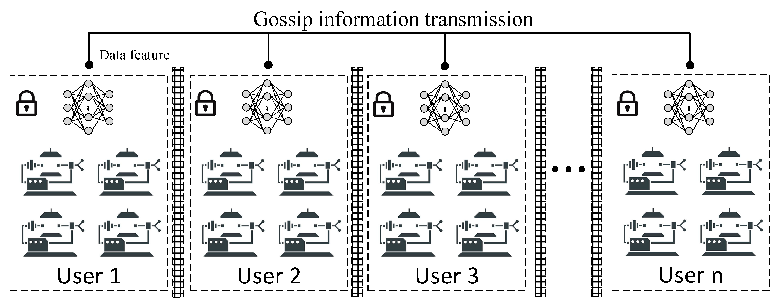
The process of DFL is shown in Figure 2. Assuming there are n clients participating in the decentralized federated learning training process, the process of DFL is as follows:
Step 1: Build a DFL framework between clients, configure relevant parameters, and protocols.
Step 2: Each client undergoes several rounds of local training;
Step 3: Randomly select a client Ci to act as a temporary central node, and transmit information through the Gossip protocol;
Step 4: Select some clients from the remaining clients to participate in the update;
Step 5: After receiving the information from other clients, Ci aggregates local and received model parameters to obtain an aggregated model, and finally sends the aggregated model parameters to all clients. The aggregated model will continue to participate in the training as the local model for the next round.
Step 6: Reread Steps 3 to 6 until the global model meets the convergence criterion. In this process, information is indirectly exchanged between clients via model updates, while all training occurs locally, thereby effectively preserving data privacy.
The parameter aggregation in the temporary central node can be expressed as
w i t + 1 = 1 K i t k K i t w k t
where w k t represents the local model parameters of client Ci in the t-th communication round, K i t represents the set of local and communication objects of client Ci in the t-th communication round, K i t represents the number of K i t , and w i t + 1 represents the aggregation model of client Ci, which is also the local model of the (t+1)-th communication round.
The core of implementing decentralization in the DFL mentioned above lies in the Gossip method. The Gossip method is a distributed information propagation mechanism based on random communication, and its working principle can be systematically explained as follows: the protocol achieves information propagation through periodic random interactions between nodes, and each node randomly selects several neighboring nodes for information exchange on a regular basis. This process includes pushing the node’s own information and receiving information from neighboring nodes. This random selection mechanism effectively avoids the solidification of information propagation paths, while the protocol adopts a regular update strategy to ensure information timeliness and maintains system consistency through a bidirectional transmission mechanism. It is worth noting that the protocol has significant fault tolerance characteristics, and even in the event of partial node failure, information can still be reliably propagated through redundant paths. Based on the above mechanism, the Gossip method can achieve efficient information diffusion in distributed systems, while ensuring the scalability and robustness of the system, ultimately achieving consistency and synchronization of node states.

3.2. Proposed Lightweight Transformer Architecture

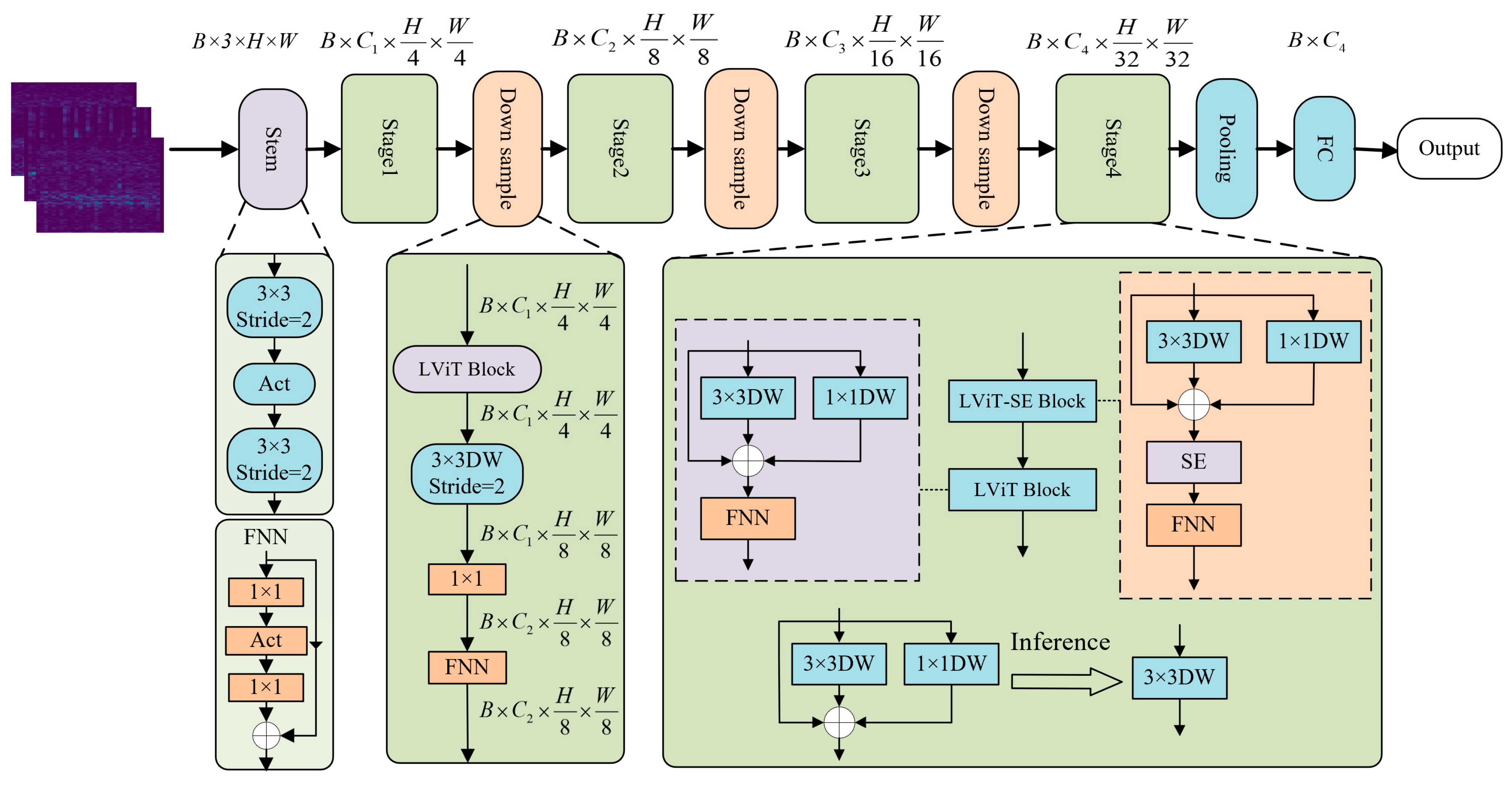
In the proposed DFed-LT-based FD approach, the lightweight transformer (LT) network is designed as local models. As shown in Figure 3, the LT includes a starting convolution, downsampling layers, pooling layers, a fully connected layer, and four integrated stages. The starting convolution, downsampling layers, and classifier are redesigned from MobileNetV3 to meet transformer design needs.

3.2.1. Stem Module

The Stem module serves as the initial processing unit at the input stage of the network, positioned at the very beginning of the entire architecture. Its primary role is to perform preliminary feature extraction and dimensionality reduction on the raw input images. It accomplishes this by employing a series of fundamental components, such as convolutional layers and pooling layers, to extract low-level features from the input images—namely, basic visual patterns like edges and textures. The stem is a critical component in transformers that processes inputs by dividing them into non-overlapping patches, traditionally implemented through large-kernel, large-stride convolutions such as a 16 × 16 convolution with stride 16, which has been shown in prior work to be essential for addressing optimization challenges in transformer-based models like Vision Transformer. This paper introduces a redesigned stem that replaces conventional large convolutions with a sequence of two 3 × 3 convolutions, each with stride 2, which are referred to as early convolutions—a modification that significantly enhances optimization stability. For input images of size 3 × H × W, this stem architecture transforms them into 48 × H 4 × W 4 patches, with the computational procedure described as follows.
F 0 = C o n v 3 × 3 C o n v 3 × 3 X R 48 × H 4 × W 4
where C o n v 3 × 3 represents the convolution operation using 3 × 3 kernels.

3.2.2. Stage Module

The Stage module adopts a hierarchical design akin to the Feature Pyramid Network (FPN), establishing multi-resolution feature output layers at varying depths within the network. Its core functionality lies in enabling multi-scale feature fusion and semantic information enhancement. The Stage architecture consists of a VCSEBlock and a VCBlock. The VCSEBlock draws inspiration from MobileNetV3’s design principles, which employs two crucial components for transformer efficiency: the token mixer (TM) for spatial information fusion using 3 × 3 depthwise convolution (DWConv), and the channel mixer (CM) for cross-channel interaction through a 1 × 1 expansion convolution followed by a 1 × 1 projection layer. The standard MobileNetV3 block positions the expansion and projection layers at its input and output stages, with the DWConv operation and an optional squeeze-and-excitation (SE) layer [40] in between, all wrapped in a residual connection. DWConv is an efficient convolution operation proposed by Google [41] in the MobileNet series of networks, which is widely used in model lightweighting research. It can significantly reduce computational and parameter complexity while maintaining the model’s feature extraction ability as much as possible. In addition, SE can explicitly model the interdependence between feature channels, adaptively recalibrate channel feature responses, thereby improving the network’s utilization efficiency of important features, enhancing the network’s feature representation ability, and ultimately improving the model’s performance in various tasks.
The VCBlock reorganizes these components by relocating the 3 × 3 DWConv to an earlier stage, followed by the optional SE module, while consolidating the expansion and projection layers in the latter half of the block. The residual connection is also modified to link the input and output of the CM exclusively. This architectural variation gives rise to two distinct blocks: the VCSEBlock (with SE layer) and VCBlock (without SE layer). Given an input feature map F 1 R C 1 × H 1 × W 1 , their respective outputs are formally expressed in Equations (5) and (6).
F T M = κ 3 × 3 F 1 + κ 1 × 1 F 1 + F 1
F S E = Ψ ( F T M )
F V C S E B = κ 1 × 1 κ 1 × 1 F S E + F S E    R C 1 × H 1 × W 1
F V C B = κ 1 × 1 κ 1 × 1 F T M + F T M    R C 1 × H 1 × W 1
where κ 1 × 1 denotes the depthwise convolution using 1 × 1 kernels, while Ψ symbolizes the SE operation process that will be elaborated subsequently. A critical parameter in the channel mixer (CM) is the expansion ratio (ER), defined as the ratio between the hidden dimension and input dimension of CM. While MobileNetV3 typically sets this parameter to 4 by default, resulting in significant computational overhead, our LFDNet addresses this efficiency challenge by strategically reducing the ER to lower computational complexity. To compensate for potential performance impacts, we correspondingly increase the network width. The experimental section will provide detailed validation of this parameter optimization approach and its effects on model performance.
The input feature F T M with dimensions C 1 × H 1 × W 1 undergoes sequential processing through the SE layer. Initially, global average pooling (GAP) is applied in the squeeze phase to transform the spatial dimensions (W × H × C) into channel-wise descriptors (1 × 1 × C), generating compressed channel statistics Z that capture global contextual information while reducing channel dependencies. This compressed representation then passes through a dimensionality-reducing fully connected (FC) layer, followed by ReLU activation and subsequent FC layer for channel dimension restoration. A sigmoid activation normalizes the output to [0, 1] range, producing channel-wise attention weights (1 × 1 × C). These weights are element-wise multiplied with the original F T M features to yield the refined output F S E . This attention mechanism adaptively modulates feature importance by amplifying relevant channels and suppressing less informative ones, thereby enhancing feature discriminability through learned channel-wise scaling.

3.2.3. Downsample Module

Downsampling plays a crucial role in deep learning architectures by reducing feature map resolution to decrease computational overhead and memory requirements. Inspired by residual networks that implement downsampling through stride-2 convolutions (3 × 3 in the main path and 1 × 1 in shortcut connections at each stage’s beginning); LT employs an enhanced downsampling module combining 3 × 3 depthwise convolution and 1 × 1 convolution. To preserve richer feature representations, the design incorporates dual stacked 1 × 1 convolutions with a residual connection. Furthermore, a VCBlock is integrated at the module’s entry point to mitigate information loss during resolution reduction through network depth increase. Given input feature F 1 R C 1 × H 1 × W 1 , the VCBlock maintains dimensional consistency, while the subsequent depthwise convolution produces C 1 × H 1 2 × W 1 2 features. The module’s final output preserves this reduced spatial dimension while maintaining channel count, with its mathematical formulation expressed as
F 2 = C o n v D W C o n v ( Φ ( F 1 ) ) + C o n v C o n v ( C o n v ( D W C o n v ( Φ ( F 1 ) ) ) )
where Φ indicates the VCBlock. D W C o n v represents the 3 × 3 depthwise convolution.

3.2.4. Classifier Module

The classifier is used to receive the features extracted by the above modules and map them to predefined categories. The classifier module employs a two-stage processing pipeline comprising global average pooling (GAP) followed by a fully connected (FC) layer. The GAP operation first compresses spatial information by computing channel-wise averages, transforming the input feature map into a compact 1-dimensional vector while preserving the original channel dimensionality. This condensed representation then undergoes linear transformation through the FC layer to produce final class predictions. The classification procedure can be mathematically represented as
Y = F C ( ρ ( F 3 ) )

4. Experiments and Result Analysis

All experimental procedures are executed on a workstation equipped with an NVIDIA GeForce RTX 3090 GPU for computational processing.

4.1. Experimental Setup and Data Description

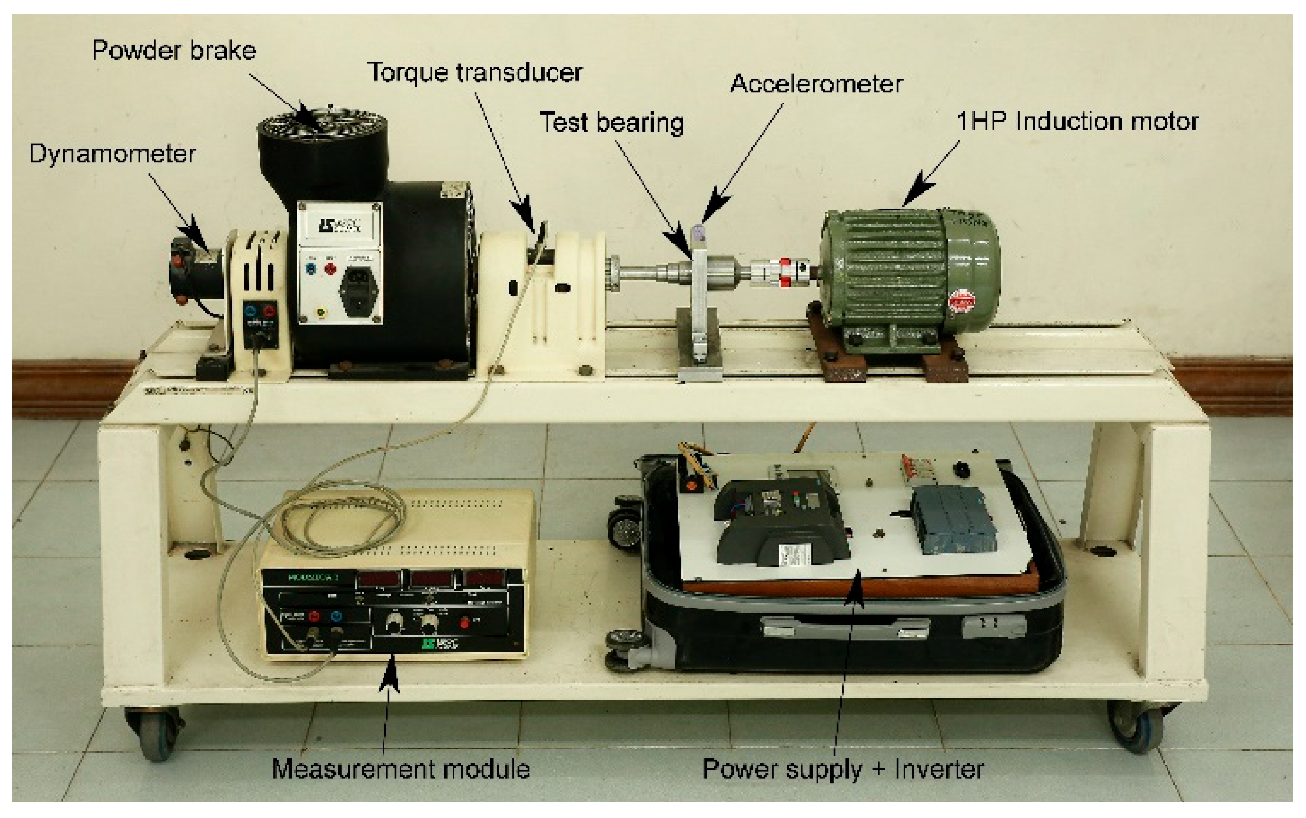
The proposed FD method is validated using the HUST bearing dataset [42], collected from the standardized test platform shown in Figure 4. The experimental setup consists of a 750 W induction motor driving a multi-step shaft system, with loading conditions simulated by a Leroy Somer powder brake controlled through an inverter. For system monitoring, a torque transducer and dynamometer ensure accurate measurement of motor load and speed. Vibration data acquisition is achieved through a vertically mounted PCB325C33 accelerometer installed on tested bearings that are flexibly coupled to the shaft.
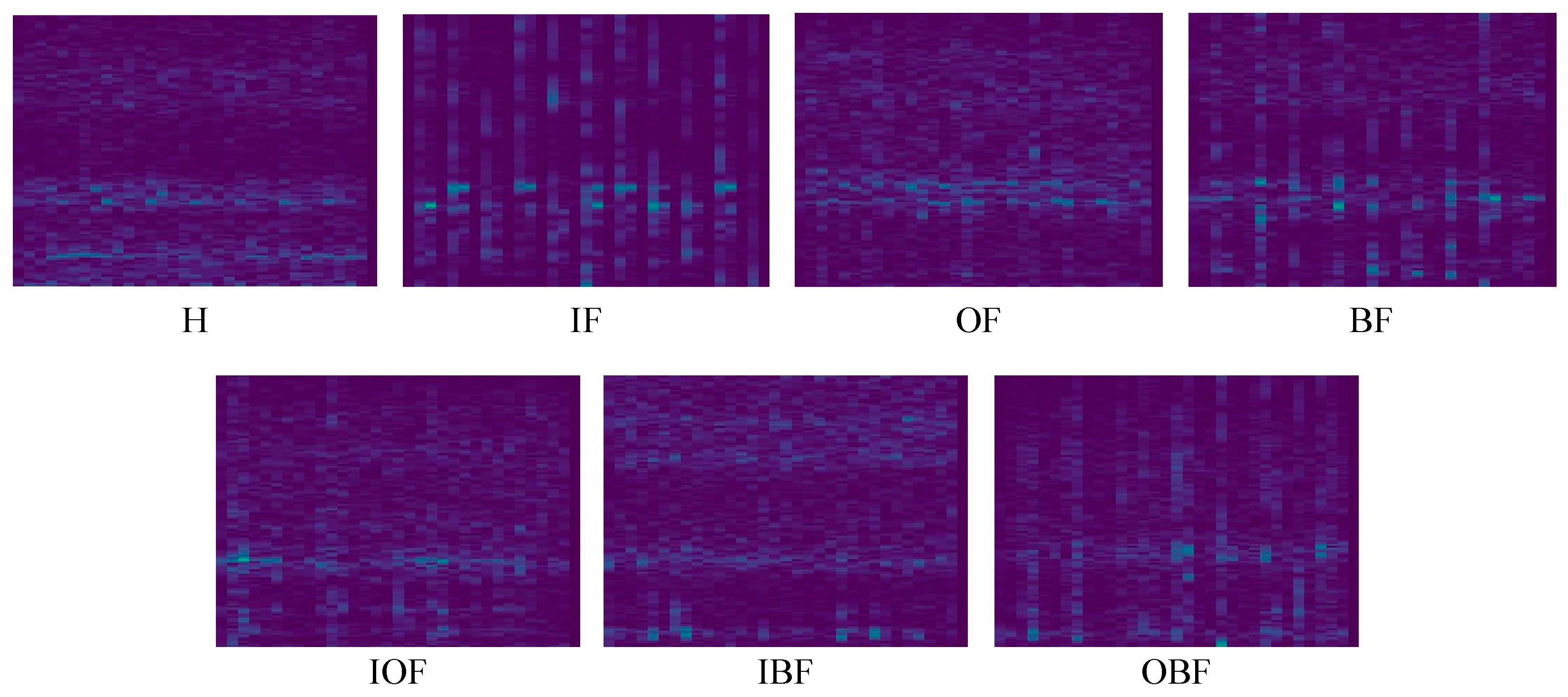
This dataset contains the vibration signals representing health (H) and six types of faults, i.e., inner faults (IFs), outer faults (OFs), ball faults (BFs), inner faults and outer faults (IOFs), inner faults and ball faults (IBFs), and outer faults and ball faults (OBFs), which are naturally damaged by accelerated life tests. Figure 5 shows the photos of various fault types. Each signal is recorded at a sampling rate of 51.2 kHz for a duration of 10 s. The data acquisition system is meticulously engineered to ensure high reliability. For each health condition, all acquired signals are cut into multiple signals samples with the same length. The specific sample information is shown in Table 3. To enable the FD model to better analyze vibration data, the raw signals are transformed into two-dimensional time–frequency representation through short time Fourier transform (SFTF), following the method in the literature [4,43]. The time–frequency spectrograms after the STFT conversion are shown in Figure 6.

4.2. Experiment 1: Fault Diagnosis Experiment Result Based on LT

4.2.1. Data Processing and Evaluation Indicators

In this part, the LT is first adopted to implement the FD task, and the HUST bearing dataset is employed. In the experiment, all the data samples are adopted and divided into three subsets: 80% of the signal samples were allocated for training, while the remaining 20% were equally split between validation and testing sets (10% each).
In addition, in order to effectively measure and compare the performance of the model, some evaluation indicators have been adopted, including accuracy, precision, recall, and F1 score, param, FLOPs. The first four indicators are classic indicators used for classification tasks [44,45,46], and their formulas are shown in Equations (9)–(12). Furthermore, the param and FLOPs are utilized to measure the model complexity and diagnostic speed for testing samples, which indicates the learnable parameter number and floating-point operations, respectively.
A c c u r a c y = T P + T N T P + F P + T N + F N
P r e c i s i o n = T P T P + F P
R e c a l l = T P T P + F N
F 1   s c o r e = 2 × P r e c i s i o n × R e c a l l P r e c i s i o n + R e c a l l
where TP, TN, FP, and FN represent the quantities of true positives, true negatives, false positives, and false negatives, respectively.

4.2.2. The Effect of Hyperparameters

The hyperparameters of the LT model undergo multiple iterations and optimizations, and we have established the final hyperparameter configuration for the LT model. The architecture employs a 1:1:5:1 stage ratio with progressive network widths of [48, 96, 192, 384] channels across stages. SE layers are strategically positioned in the first block of each stage to enhance feature representation. For model optimization, we utilize the Adam optimizer with Gaussian Error Linear Units (GeLUs) serving as the activation function throughout the network. Specifically, many model hyperparameters significantly influence diagnostic performance, including the expansion ratio of CM, network width of CM, SE layer configuration in VCSEBlock, and others. During training, these hyperparameters are continuously tuned and optimized to improve model effectiveness. The verification experiment is conducted to determine the optimal hyperparameters, and the specific process is as follows.
(1)
The Effect of Expansion Ratio of CM
As introduced previously, the expansion ratio is defined as the ratio of hidden dimension to input dimension in the CM. This hyperparameter critically influences both the feature transformation capability of the CM and the overall FD performance of the model. Therefore, different expansion ratios are tested and explored, including 2, 3, and 4. Figure 7 compares the performance metrics and computational efficiency under different expansion ratios, specifically showing the trend of changes as the expansion ratio increases from 2 to 4. In terms of model performance, when the expansion ratio is 2, the model achieved 98.41% accuracy, 98.23% precision, 98.27% recall, and 98.25% F1 score; after increasing the expansion ratio to 3, all indicators showed slight improvements, reaching 98.43%, 98.39%, 98.33%, and 98.36%, respectively; when using the maximum expansion ratio of 4, the model achieves optimal performance, with an accuracy improvement of 98.49%, while maintaining high precision (98.38%) and recall (98.42%), and the F1 score correspondingly increases to 98.40%. In terms of computational resource consumption, as the expansion ratio increases, the number of model parameters (params) linearly increases from 2.47 million (2.47 M) to 2.69 M (ratio 3) and 2.91 M (ratio 4), and the corresponding floating-point operations (FLOPs) also significantly increase from 8.57 G to 9.44 G and 10.35 G. It is obvious that increasing the expansion ratio will impact the deployability and usability of the model on edge devices in real-world scenarios. Overall, although the improvement in expansion ratio can slightly optimize model performance, it comes at the cost of higher computational costs. Therefore, in engineering practice, it is necessary to balance the requirements of accuracy and efficiency based on specific tasks. In this paper, the expansion ratio is ultimately set to 3.
(2)
The Effect of Network Width
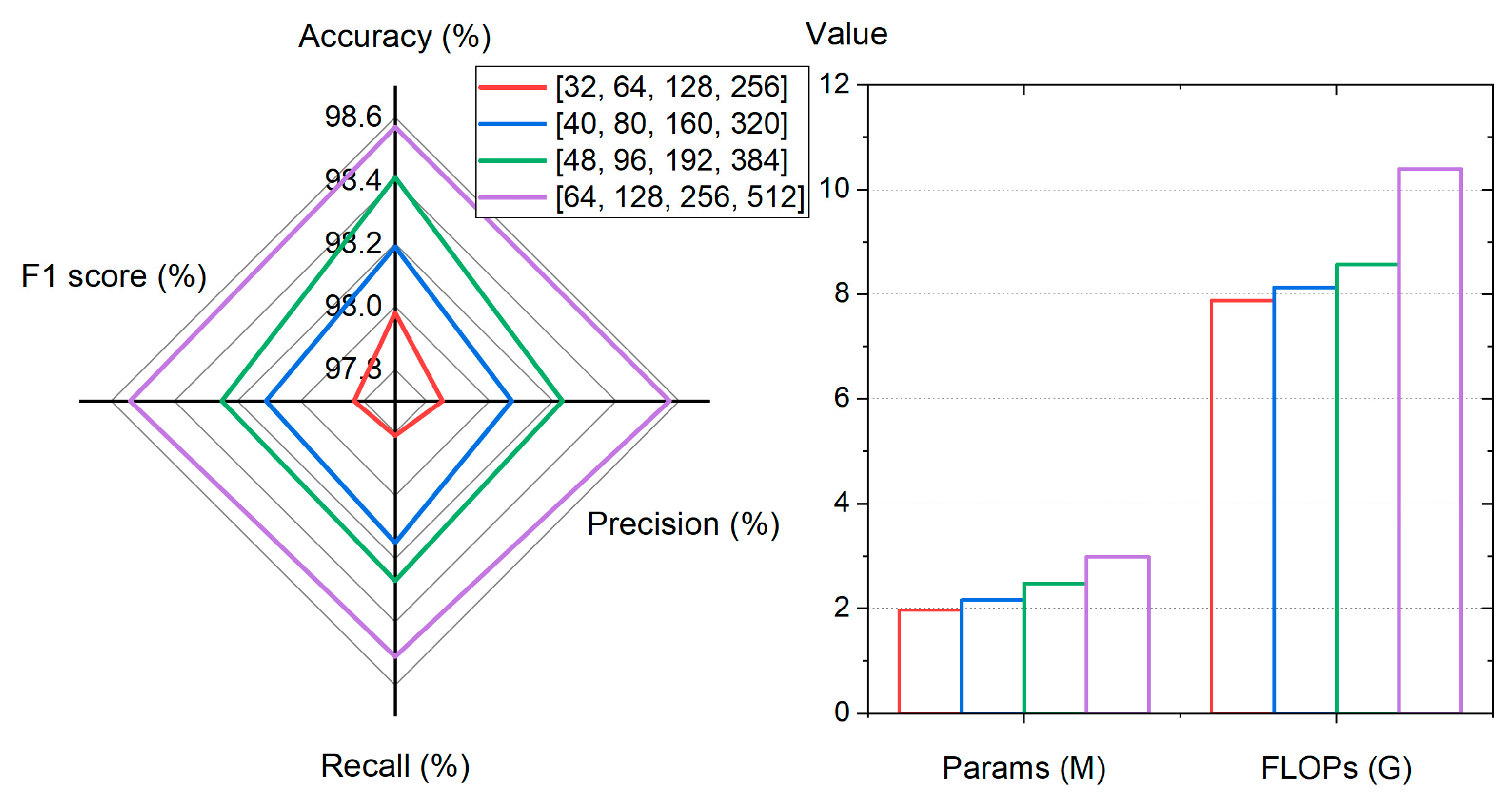
Network width is also an important factor in model settings. We compared the performance and computational resource consumption of LT models under different network width configurations. Four gradually increasing channel configuration schemes were experimentally tested, namely [32, 64, 128, 256], [40, 80, 160, 320], [48, 96, 192, 384], and [64, 128, 256, 512]. The result is shown in Figure 8. In terms of model performance, as the network width increases, various evaluation indicators show a stable improvement trend: when using the narrowest [32, 64, 128, 256] configuration, the model accuracy is 97.98%, precision is 97.85%, recall is 97.81%, and F1 score is 97.83%; When the width is expanded to [48, 96, 192, 384], the four indicators increase to 98.41%, 98.23%, 98.27%, and 98.25%, respectively; When using the widest configuration [64, 128, 256, 512], the model achieved optimal performance, with an accuracy rate of 98.57%, and precision rate and F1 score of 98.57% and 98.54%, respectively. The recall also increased to 98.51%, indicating a significant positive correlation between network width and model performance. It can be easily deduced that this phenomenon would persist even in real-world application scenarios. In terms of computational efficiency, the number of model parameters (params) gradually increased from 1.97 M to 2.98 M, and FLOPs also increased from 7.88 G to 10.39 G, indicating that a wider network structure will significantly increase computational overhead, thereby reducing its availability in edge devices. The experimental results indicate that although increasing network width can effectively improve model performance, it is necessary to balance the consumption of computing resources. Taking into account both model performance and computational resources, the network width of LT in this paper is set to [48, 96, 192, 384].
(3)
The Effect of SE layer Configurations
The impact of SE layer on model performance has also been studied. Figure 9 systematically compares the impact of four different SE layer configurations on the performance and computational efficiency of the LT model, where “1 √” indicates that the SE layer is configured in the first block (i.e., the block is VCSEBlock), and “2 ×” indicates that the SE layer is not configured in the second block (i.e., the block is VCBlock). Four configuration schemes were set up in the experiment: Configuration 1 (both blocks were not enabled) was used as the baseline model, with an accuracy of 97.29%, precision of 97.22%, recall of 97.26%, and F1 score of 97.24%; when only the second block is enabled (configuration 2), the model performance significantly improves, with four indicators reaching 98.41%, 98.23%, 98.27%, and 98.25%, respectively; when only the first block is enabled (Configuration 3), it also brings significant improvements, with indicators of 98.37%, 98.19%, 98.21%, and 98.20%; when two blocks (Configuration 4) are simultaneously enabled, the model achieves optimal performance, with an accuracy improvement of 98.43%, an accuracy and F1 score of 98.41% and 98.37%, respectively, and a recall rate of 98.33%. But compared to Configurations 2 and 3, the performance improvement is not significant. In terms of computing resources, the baseline configuration has a parameter number of 2.38 M and floating point operations (FLOPs) of 7.96 G. As the block is enabled, the computational cost gradually increases, and the full configuration (Configuration 4) reaches its maximum resource consumption (2.56 M parameters and 8.89 G FLOPs). While the incorporation of SE layers demonstrates substantial performance improvements, our experiments reveal that dual-SE block configuration fails to deliver commensurate benefits while unnecessarily increasing model complexity. This empirical finding motivates our selection of Configuration 2 as the optimal architecture for the LT model.

4.2.3. Diagnostic Results and Performance Comparison

The diagnostic results of proposed LT model are compared with that of other models performing the same diagnostic task, including CNN, Uniformer, and MobileNetV3. The FD results for all models are shown in Table 4. By comparing the results in the table, the following conclusions can be drawn:
(1)
In terms of classification performance, traditional CNN models have relatively low performance, with four indicators accounting for about 85%. MobileNetV3 performs stably, with all indicators reaching over 97%; Uniformer is relatively good, with all four indicators exceeding 98%. Among all models, the LT model performed the best, with significantly higher accuracy (99.06%), precision (99.17%), recall (98.87%), and F1 score (99.02%) compared to other models.
(2)
In terms of computational efficiency, the CNN model has the lowest parameter number (0.06 M) and FLOPs (1.52 G), but the performance gap is significant; the LT model achieved higher classification performance and better performance balance, with significantly lower parameter number (2.48 M) and FLOPs (8.58 G) compared to the Uniformer (20.89 M/127.69 G); the computational cost of MobileNetV3 (2.92 M/10.87 G) is similar to that of the LT model, but its performance is slightly inferior.
(3)
The LT model can achieve excellent diagnostic performance similar to larger models such as Uniformer, while also having relatively low model complexity. This makes it highly suitable in engineering applications with limited computing resources.

4.3. Experiment 2: Fault Diagnosis Experiment Result Based on DFed-LT

This experiment is based on the assumption that multiple clients utilize identical bearing models, with each client independently collecting monitoring data to form their respective private datasets. To simulate this distributed data scenario under privacy-preserving conditions, we systematically partitioned all samples from the HUST-bearing dataset into non-overlapping subsets, each representing an individual client’s private data.
The DFed-LT is utilized to implement this FD task. The model parameters are configured as follows: the SGD (Stochastic Gradient Descent) optimization algorithm is employed as the optimizer with an initial momentum of 0.0001. The local model undergoes three training iterations, while the global model is trained for five hundred iterations. The learning rate is set to 0.001, and the batch size is configured as 32.
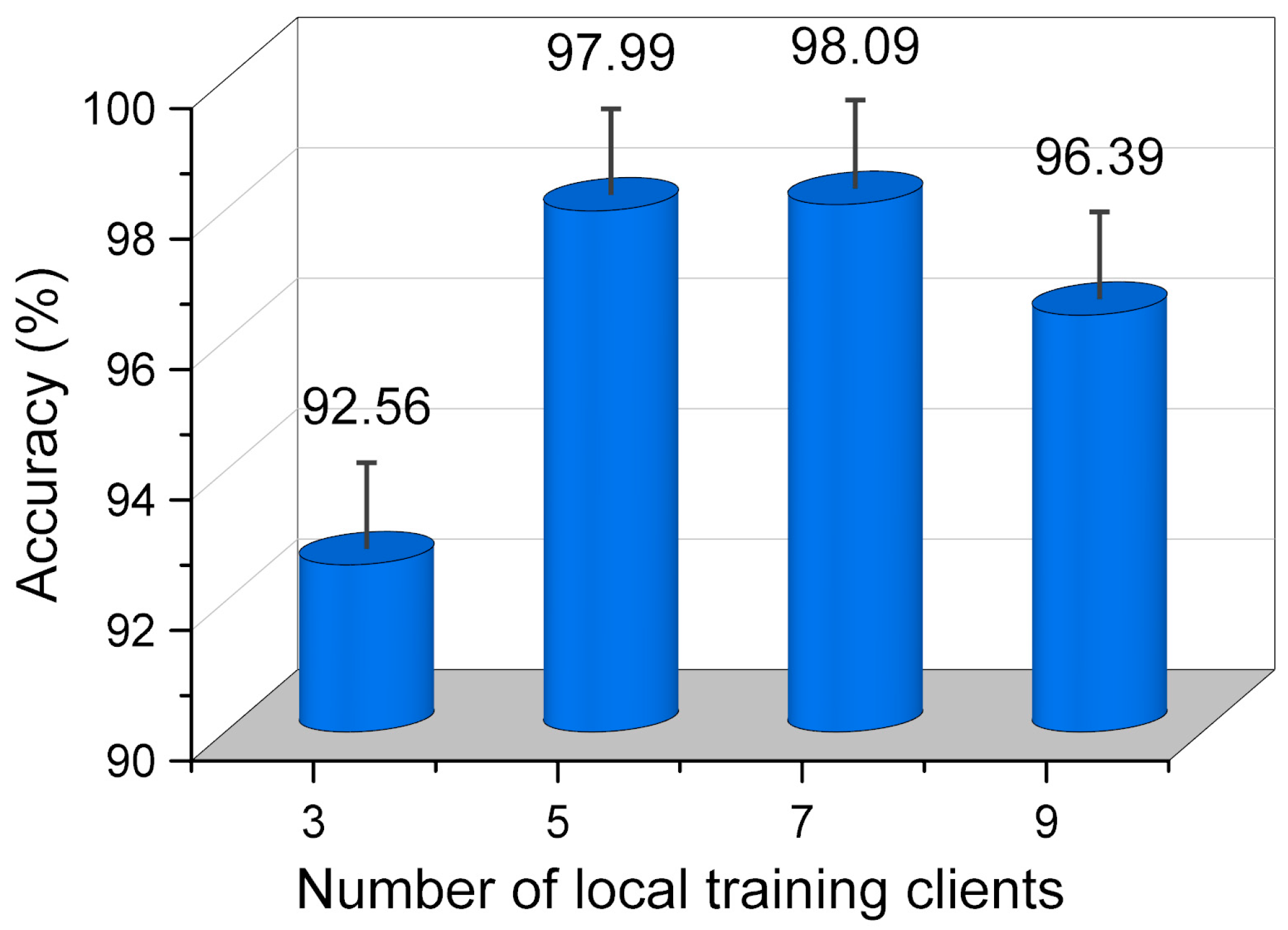
To assess the stability of classification accuracy, each experimental condition was independently replicated five times. The system was configured with a fixed pool of 10 client nodes, while the number of randomly selected participants for local training systematically varied across {three, five, seven, nine} to evaluate scaling effects. As demonstrated in Figure 10, classification accuracy exhibits a positive correlation with the number of participating clients. The optimal performance (peak accuracy) occurs with seven active clients, suggesting an ideal trade-off between data diversity benefits and the computational efficiency of distributed training.
The training results from one trial are presented in Figure 11. As shown, the proposed DFed-TL converges after approximately 300 training cycles. Throughout the training process, the training accuracy exhibits a consistent upward trend. Across five independent trials, the model achieves an average validation accuracy of 98.19% with a standard deviation of 1.25%.
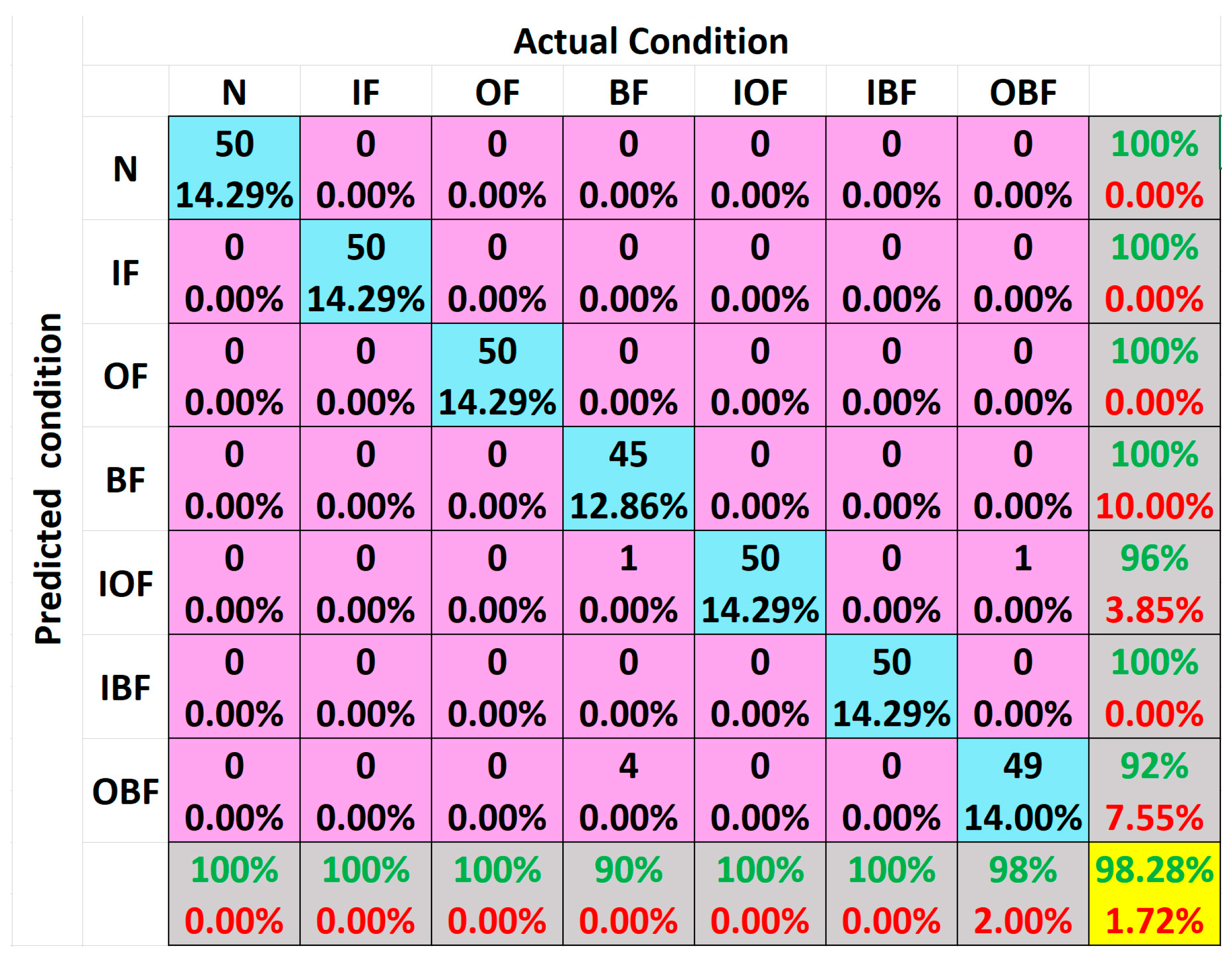
The confusion matrix of the diagnostic results is presented in Figure 12, which shows that the proposed method achieved perfect classification (100% accuracy) for most categories, except for a small number of misclassified test samples in the BF and OBF categories. These results demonstrate the method’s strong classification capability and its consistent predictive accuracy across different fault types.
To further evaluate the performance of the proposed method, several methods were adopted for performance comparison, including the following:
  • Non-Fed: Non-federated, whereby each local client trains a local model for local diagnosis, and the final result is the average of each local diagnostic model.
  • FedAvg-CNN: A federated learning approach using the Federated Average (FedAvg) framework with CNN as the local model.
  • DFed-CNN: A decentralized federated learning approach with CNN as the local model.
  • FedAvg-LT: This model is based on the FedAvg framework with LT as the local model.
Table 5 summarizes the testing accuracy of the proposed DFed-LT and the other four comparison methods. The following observations can be made:
(1)
The non-fed (non-federated learning) baseline method demonstrated the poorest performance (average accuracy: 51.34%, F1-score: 52.02%), indicating that individual local models struggle to achieve accurate diagnostic performance when trained on limited and isolated data samples.
(2)
Comparative analysis of FedAvg-CNN, DFed-CNN, FedAvg-LT, and DFed-LT reveals that employing the LT model as the local model yields significantly superior diagnostic performance compared to using CNN as the local model, further validating the enhanced feature extraction capability of the LT architecture. From an engineering perspective, the LT model’s scalability and efficiency in handling complex feature interactions make it more suitable for resource-constrained edge devices. Its balanced trade-off between computational cost and performance enhancement ensures practical deployability in real-world federated systems.
(3)
Methods utilizing the DFed framework consistently outperformed their FedAvg counterparts in diagnostic accuracy, statistically confirming the advantages and practical applicability of our proposed decentralized federated learning approach. The decentralized design eliminates single-point bottlenecks and enhances system robustness, making it ideal for large-scale or privacy-sensitive engineering scenarios.
(4)
The proposed DFed-LT method achieved optimal diagnostic performance (accuracy: 98.29%, F1-score: 99.28%) while maintaining data privacy, demonstrating its significant superiority over alternative methods in privacy-preserving medical diagnosis scenarios.

4.4. Experiment 3: Fault Diagnosis Experiment Result Based on DFed-LT in Noisy Environments

To verify the robustness of the model in strong noise environments, noise robustness experiments were conducted. By following refs. [4,20], the Gaussian white noise was added to original vibration samples to simulate noise samples, with signal-to-noise ratio (SNR) as 8, 4, 0, and −4 dB.
Table 6 evaluates the robustness of distinct methods under progressively challenging SNR conditions. It can be seen that
(1)
A clear and consistent trend observed across all methods is the monotonic decrease in diagnostic accuracy as the noise level increases. This inverse relationship between SNR and performance underscores the significant challenge that environmental noise poses to model stability and confirms that noise robustness is a critical metric for evaluating practical applicability. The performance degradation is most pronounced at the extreme noise level of −4 dB, where all methods exhibit their lowest accuracy scores.
(2)
Among the methods compared, the Non-Fed consistently demonstrates the poorest performance and robustness across the entire noise spectrum. Its accuracy declines from 48.21% at 8 dB to 34.62% at −4 dB. This substantial performance drop highlights the inherent limitation of models trained in isolation on limited local data, which fail to learn generalized and noise-invariant features, making them highly vulnerable to data corruption and unsuitable for real-world deployments where signal quality can vary significantly.
(3)
When comparing the federated learning approaches, a clear hierarchy of performance emerges based on the underlying model architecture and federation strategy. Methods utilizing the LT model as a local client consistently and significantly outperform those based on the CNN architecture at every SNR level. For instance, at 0 dB, FedAvg-LT (86.33%) surpasses DFed-CNN (68.59%) by a considerable margin. This pronounced performance gap, maintained even under high noise, provides strong evidence for the superior feature extraction and representation learning capacity of the LT architecture, which is evidently more resilient to signal degradation.
(4)
Within each architectural class, a consistent advantage is observed for the DFed framework over its FedAvg counterpart. This is illustrated by DFed-CNN (79.65% at 8 dB) outperforming FedAvg-CNN (76.88% at 8 dB) and, most importantly, by the proposed DFed-LT method achieving the top accuracy at every noise level. The DFed-LT method registers the highest recorded accuracies, from 95.85% at 8 dB to 81.28% at −4 dB. This result statistically validates the synergistic effect of combining the robust LT model with the decentralized federated learning (DFed) strategy, culminating in a system that excels in both performance and noise robustness.
In conclusion, the results demonstrate that the proposed DFed-LT method represents the most robust and reliable approach for diagnostic tasks in noisy environments. Its leading performance across all tested conditions, especially under severe noise corruption, confirms its practical superiority and suggests a stronger capability for generalization in real-world scenarios where data cleanliness cannot be guaranteed.

5. Conclusions

This study proposes a decentralized federated learning approach incorporating transformer networks to address two critical challenges in deep learning-based fault diagnosis: data privacy constraints that prevent centralized data aggregation, and hardware limitations of edge devices that restrict complex model deployment. The developed framework establishes a distributed learning architecture that preserves data privacy while enabling collaborative feature learning across multiple users. Key innovations include the implementation of a lightweight transformer network as a local model, ensuring compatibility with resource-constrained devices. In the verification experiment, the LT model achieved a diagnostic accuracy of 99.06% in fault diagnosis tasks. Even under data privacy protection, the proposed DFed LT method can still achieve a diagnostic accuracy of 98.27%, which is much higher than other conventional approaches. Experimental results demonstrate the method’s effectiveness in achieving accurate fault diagnosis while maintaining data confidentiality.
Although the current research on lightweight transformer local models is adapted to edge devices, it has not fully evaluated the impact of edge devices with different hardware configurations (such as sensors and controllers with different computing power) in industrial environments on model deployment compatibility and training efficiency. Another limitation is that this article only validated the effectiveness of the proposed method in one case, lacking validation in practical scenarios.
In the future, we will implement the application of this method in practical fields and also attempt to extend the framework to more industrial equipment (such as wind turbines and power equipment) to verify its generalization and universality.

Author Contributions

Writing—original draft preparation and methodology, K.X.; software, C.C.; data analysis and writing—review and editing, Y.C.; visualization, Y.W.; supervision, L.C.; funding acquisition, W.W. and W.S. All authors have read and agreed to the published version of the manuscript.

Funding

This research was funded by National Natural Science Foundation of China (Nos. 62476259 and 52405567), Guang-dong Basic and Applied Basic Research Foundation (Nos. 2023A1515240022 and 2024A1515140090), Natural Science Foundation of Hubei Province (No. 2024AFB023), Foundation of Guangdong Provincial Key Laboratory of Manufacturing Equipment Digitization (2023B1212060012), Shenzhen Natural Science Foundation (JCYJ20240813113102003).

Data Availability Statement

Data will be made available on request.

Conflicts of Interest

Authors Wen Wen and Wei Shang were employed by the China Railway Science & Industry Group Equipment Engineering Co., Ltd. The remaining authors declare that the research was conducted in the absence of any commercial or financial relationships that could be construed as a potential conflict of interest.

References

  1. Lv, Y.; Yang, X.; Li, Y.; Liu, J.; Li, S. Fault detection and diagnosis of marine diesel engines: A systematic review. Ocean Eng. 2024, 294, 116798. [Google Scholar] [CrossRef]
  2. Liang, P.; Tian, J.; Wang, S.; Yuan, X. Multi-source information joint transfer diagnosis for rolling bearing with unknown faults via wavelet transform and an improved domain adaptation network. Reliab. Eng. Syst. Saf. 2024, 242, 109788. [Google Scholar] [CrossRef]
  3. Li, G.; Wu, J.; Deng, C.; Xu, X.; Shao, X. Deep reinforcement learning-based online domain adaptation method for fault diagnosis of rotating machinery. IEEE/ASME Trans. Mechatron. 2022, 27, 2796–2805. [Google Scholar] [CrossRef]
  4. Cheng, Y.; Lin, X.; Liu, W.; Zeng, M.; Liang, P. A local and global multi-head relation self-attention network for fault diagnosis of rotating machinery under noisy environments. Appl. Soft Comput. 2025, 176, 113138. [Google Scholar] [CrossRef]
  5. Yuan, M.; Zeng, M.; Rao, F.; He, Z.; Cheng, Y. An interpretable algorithm unrolling network inspired by general convolutional sparse coding for intelligent fault diagnosis of machinery. Measurement 2025, 244, 116332. [Google Scholar] [CrossRef]
  6. Yang, Z.; Wang, X.; Zhong, J. Representational learning for fault diagnosis of wind turbine equipment: A multi-layered extreme learning machines approach. Energies 2016, 9, 379. [Google Scholar] [CrossRef]
  7. Bhole, N.; Ghodke, S. Motor Current Signature Analysis for Fault Detection of Induction Machine–A Review. In Proceedings of the 2021 4th Biennial International Conference on Nascent Technologies in Engineering (ICNTE), NaviMumbai, India, 15–16 January 2021; pp. 1–6. [Google Scholar]
  8. Bayma, R.S.; Lang, Z.Q. Fault diagnosis methodology based on nonlinear system modelling and frequency analysis. IFAC Proc. 2014, 47, 8278–8285. [Google Scholar] [CrossRef]
  9. Alwodai, A.; Wang, T.; Chen, Z.; Gu, F.; Cattley, R.; Ball, A. A Study of Motor Bearing Fault Diagnosis using Modulation Signal Bispectrum Analysis of Motor Current Signals. J. Sig. Inform. Proc. 2013, 4, 72–79. [Google Scholar] [CrossRef]
  10. Ma, C.; Zhang, W.; Shi, M.; Zou, X.; Xu, Y.; Zhang, K. Feature identification based on cepstrum-assisted frequency slice function for bearing fault diagnosis. Measurement 2025, 246, 116753. [Google Scholar] [CrossRef]
  11. Kankar, P.K.; Sharma, S.C.; Harsha, S.P. Fault diagnosis of ball bearings using continuous wavelet transform. Appl. Soft Comput. 2011, 11, 2300–2312. [Google Scholar] [CrossRef]
  12. Ma, K.; Wang, Y.; Yang, Y. Fault Diagnosis of Wind Turbine Blades Based on One-Dimensional Convolutional Neural Network-Bidirectional Long Short-Term Memory-Adaptive Boosting and Multi-Source Data Fusion. Appl. Sci. 2025, 15, 3440. [Google Scholar] [CrossRef]
  13. Dladla, V.M.N.; Thango, B.A. Fault Classification in Power Transformers via Dissolved Gas Analysis and Machine Learning Algorithms: A Systematic Literature Review. Appl. Sci. 2025, 15, 2395. [Google Scholar] [CrossRef]
  14. Huang, X.; Teng, Z.; Tang, Q.; Yu, Z.; Hua, J.; Wang, X. Fault diagnosis of automobile power seat with acoustic analysis and retrained SVM based on smartphone. Measurement 2022, 202, 111699. [Google Scholar] [CrossRef]
  15. Liu, G.; Ma, Y.; Wang, N. Rolling Bearing Fault Diagnosis Based on SABO–VMD and WMH–KNN. Sensors 2024, 24, 5003. [Google Scholar] [CrossRef]
  16. Chen, J.-H.; Zou, S.-L. An Intelligent Condition Monitoring Approach for Spent Nuclear Fuel Shearing Machines Based on Noise Signals. Appl. Sci. 2018, 8, 838. [Google Scholar] [CrossRef]
  17. Liang, X.; Yao, J.; Zhang, W.; Wang, Y. A Novel Fault Diagnosis of a Rolling Bearing Method Based on Variational Mode Decomposition and an Artificial Neural Network. Appl. Sci. 2023, 13, 3413. [Google Scholar] [CrossRef]
  18. Yan, X.; Liu, Y.; Jia, M. Multiscale cascading deep belief network for fault identification of rotating machinery under various working conditions. Knowl.-Based Syst. 2020, 193, 105484. [Google Scholar] [CrossRef]
  19. Jiang, G.; Xie, P.; He, H.; Yan, J. Wind turbine fault detection using a denoising autoencoder with temporal information. IEEE/ASME Trans. Mechatron. 2018, 23, 89–100. [Google Scholar] [CrossRef]
  20. Li, G.; Wu, J.; Deng, C.; Chen, Z. Parallel multi-fusion convolutional neural networks based fault diagnosis of rotating machinery under noisy environments. ISA Trans. 2022, 128, 545–555. [Google Scholar] [CrossRef] [PubMed]
  21. Chen, Z.; Huang, H.; Deng, Z.; Wu, J. Shrinkage mamba relation network with out-of-distribution data augmentation for rotating machinery fault detection and localization under zero-faulty data. Mech. Syst. Signal Process. 2025, 224, 112145. [Google Scholar] [CrossRef]
  22. Wang, S.; Shuai, H.; Hu, J.; Zhang, J.; Liu, S.; Yuan, X.; Liang, P. Few-shot fault diagnosis of axial piston pump based on prior knowledge-embedded meta learning transformer under variable operating conditions. Expert Syst. Appl. 2025, 269, 126452. [Google Scholar] [CrossRef]
  23. Zhang, W.; Li, X.; Ma, H.; Luo, Z.; Li, X. Federated learning for machinery fault diagnosis with dynamic validation and self-super. Knowl.-Based Syst. 2021, 213, 106679. [Google Scholar] [CrossRef]
  24. Du, J.; Qin, N.; Jia, X.; Zhang, Y.; Huang, D. Fault diagnosis of multiple railway high speed train bogies based on federated learning. J. Southwest Jiaotong Univ. 2024, 59, 185–192. [Google Scholar]
  25. Zhang, Z.; Xu, X.; Gong, W.; Chen, Y.; Gao, H. Efficient federated convolutional neural network with information fusion for rolling bearing fault diagnosis. Control Eng. Pract. 2021, 116, 104913. [Google Scholar] [CrossRef]
  26. Geng, D.Q.; He, H.W.; Lan, X.C.; Liu, C. Bearing fault diagnosis based on improved federated learning algorithm. Computing 2022, 104, 1–19. [Google Scholar] [CrossRef]
  27. Wang, Q.; Li, Q.; Wang, K.; Wang, H.; Zeng, P. Efficient federated learning for fault diagnosis in industrial cloud-edge computing. Computing 2021, 103, 2319–2337. [Google Scholar] [CrossRef]
  28. Li, Y.; Chen, Y.; Zhu, K.; Bai, C.; Zhang, J. An Effective Federated Learning Verification Strategy and Its Applications for Fault Diagnosis in Industrial Iot Systems. IEEE Internet Things 2022, 9, 16835–16849. [Google Scholar] [CrossRef]
  29. Liang, Y.; Zhao, P.; Wang, Y. Federated Few-Shot Learning-Based Machinery Fault Diagnosis in the Industrial Internet of Things. Appl. Sci. 2023, 13, 10458. [Google Scholar] [CrossRef]
  30. Berghout, T.; Benbouzid, M.; Bentrcia, T.; Lim, W.H.; Amirat, Y. Federated Learning for Condition Monitoring of Industrial Processes: A Review on Fault Diagnosis Methods, Challenges, and Prospects. Electronics 2023, 12, 158. [Google Scholar] [CrossRef]
  31. Pei, X.; Zheng, X.; Wu, J. Rotating machinery fault diagnosis through a transformer convolution network subjected to transfer learning. IEEE Trans. Instrum. Meas. 2021, 70, 2515611. [Google Scholar] [CrossRef]
  32. Ding, Y.; Jia, M.; Miao, Q.; Cao, Y. A novel time-frequency Transformer based on self-attention mechanism and its application in fault diagnosis of rolling bearings. Mech. Syst. Signal Process. 2022, 168, 108616. [Google Scholar] [CrossRef]
  33. Jin, C.; Chen, X. An end-to-end framework combining time-frequency expert knowledge and modified transformer networks for vibration signal classification. Expert Syst. Appl. 2021, 171, 114570. [Google Scholar] [CrossRef]
  34. Zhou, H.; Huang, X.; Wen, G.; Dong, S.; Lei, Z.; Zhang, P.; Chen, X. Convolution enabled transformer via random contrastive regularization for rotating machinery diagnosis under time-varying working conditions. Mech. Syst. Signal Process. 2022, 173, 109050. [Google Scholar] [CrossRef]
  35. Liu, W.; Zhang, Z.; Zhang, J.; Huang, H.; Zhang, G.; Peng, M. A novel fault diagnosis method of rolling bearings combining convolutional neural network and transformer. Electronics 2023, 12, 1838. [Google Scholar] [CrossRef]
  36. Xie, F.; Wang, G.; Zhu, H.; Sun, E.; Fan, Q.; Wang, Y. Rolling bearing fault diagnosis based on SVD-GST combined with vision transformer. Electronics 2023, 12, 3515. [Google Scholar] [CrossRef]
  37. Xiao, Y.; Shao, H.; Wang, J.; Yan, S.; Liu, B. Bayesian variational transformer: A generalizable model for rotating machinery fault diagnosis. Mech. Syst. Signal Process. 2024, 207, 110936. [Google Scholar] [CrossRef]
  38. Chen, C.; Liu, C.; Wang, T.; Zhang, A.; Wu, W.; Cheng, L. Compound fault diagnosis for industrial robots based on dual-transformer networks. J. Manuf. Syst. 2023, 66, 163–178. [Google Scholar] [CrossRef]
  39. Huang, X.; Wu, T.; Yang, L.; Hu, Y.; Chai, Y. Domain adaptive fault diagnosis based on Transformer feature extraction for rotating machinery. Chin. J. Sci. Instrum. 2022, 43, 210–218. [Google Scholar]
  40. Hu, J.; Shen, L.; Albanie, S.; Sun, G.; Wu, E. Squeeze-and-Excitation Networks. IEEE Trans. Pattern Anal. 2020, 42, 2011–2023. [Google Scholar] [CrossRef]
  41. Chollet, F. Xception: Deep Learning with Depthwise Separable Convolutions. In Proceedings of the 2017 IEEE Conference on Computer Vision and Pattern Recognition (CVPR), Honolulu, HI, USA, 21–26 July 2017; pp. 1800–1807. [Google Scholar]
  42. Thuan, N.D.; Hong, H.S. HUST bearing: A practical dataset for ball bearing fault diagnosis. BMC Res. Notes 2023, 16, 138. [Google Scholar] [CrossRef]
  43. Xie, K.; Wang, C.; Wang, Y.; Cheng, Y.; Chen, L. A denoising diffusion probabilistic model-based fault sample generation approach for imbalanced intelligent fault diagnosis. Meas. Sci. Technol. 2025, 36, 066134. [Google Scholar] [CrossRef]
  44. Wen, L.; Li, X.; Gao, L. A transfer convolutional neural network for fault diagnosis based on ResNet-50. Neural Comput. Appl. 2019, 32, 6111–6124. [Google Scholar] [CrossRef]
  45. Chen, Z.; Wu, J.; Deng, C.; Wang, C.; Wang, Y. Residual deep subdomain adaptation network: A new method for intelligent fault diagnosis of bearings across multiple domains. Mech. Mach. Theory 2022, 169, 104635. [Google Scholar] [CrossRef]
  46. Liang, P.; Wang, W.; Yuan, X.; Liu, S.; Zhang, L.; Cheng, Y. Intelligent fault diagnosis of rolling bearing based on wavelet transform and improved ResNet under noisy labels and environment. Eng. Appl. Artif. Intel. 2022, 115, 105269. [Google Scholar] [CrossRef]
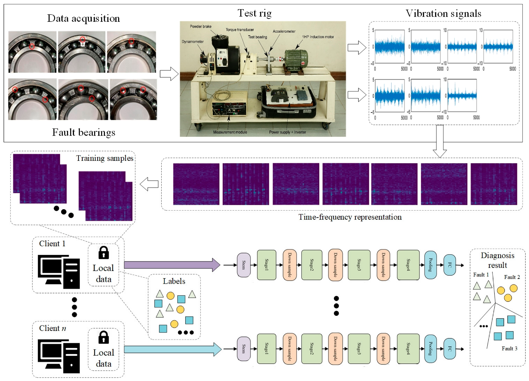
Figure 1. The overall flowchart for fault diagnosis based on DFed-LT.
Applsci 15 11484 g001
Figure 2. The framework of federated learning.
Applsci 15 11484 g002
Figure 3. The architecture of the proposed LT.
Applsci 15 11484 g003
Figure 4. Wind turbine gearbox test rig.
Applsci 15 11484 g004
Figure 5. Photos of bearing faults: (a) IF, (b) OF, (c) BF, (d) IOF, (e) IBF, and (f) OBF.
Applsci 15 11484 g005
Figure 6. Time–frequency representation of raw signal samples for various health conditions.
Applsci 15 11484 g006
Figure 7. Comparison of model performance under different expansion ratios.
Applsci 15 11484 g007
Figure 8. Comparison of model performance under different network widths.
Applsci 15 11484 g008
Figure 9. Comparison of model performance under different SE layer configurations.
Applsci 15 11484 g009
Figure 10. Test accuracy of different numbers of clients.
Applsci 15 11484 g010
Figure 11. Training process of DFed-TL.
Applsci 15 11484 g011
Figure 12. Confusion matrix.
Applsci 15 11484 g012
Table 1. Comparison of different federated learning methods for fault diagnosis.
MethodsMain FeaturesAdvantagesLimitations
[23]Dynamic validation; Self-supervisionSuitable for time series monitoring dataClient uploads risk leaks; server faults hurt fault diagnosis training; central setup hikes fault diagnosis costs
[24]Multi-scale convolutionDiverse data features
[25]Adaptive communicationLess communication rounds
[26]Optimized the global model using F1 score; increased the accuracy differenceLess communication rounds
[27]Edge picks cloud models async via local dataImproved efficiency; reduced computational and communication costs
[28]Trained using a stacked networkCombined with the Internet of Things
DFed-LTDecentralized architectureCalculates global model via node-to-node relay-
Table 2. Comparison of different transformer methods for fault diagnosis.
MethodsMain FeaturesAdvantagesLimitations
[31]Combines transformer encoder and CNNFirst application of transformer to rotating machinery FD; leverages benefits of both architecturesComplex structures; numerous learnable parameters; require substantial computational resources; difficult to deploy on edge devices
[32]Based on time–frequency transformerAddresses shortcomings of classical structures in computational efficiency and feature representation; demonstrated superiority
[33]Four-step process: data preprocessing, time–frequency feature extraction, improved transformer, integral optimizationStructured end-to-end workflow for vibration signal classification
[34]Improved self-attention via depthwise separable convolution and random comparison regularizationEnables deep transformer encoder; improves generalization under different operating conditions
[35]Balances CNN-like and transformer-like featuresAddresses limitations of CNN and strict data quality requirements of the transformer
[36]Uses visual transformerDeals with noise interference and makes better use of data features beyond 1D information
[37]Uses transformer to focus on important featuresImproves feature selection ability
[38]Combines wavelet time–frequency analysis and swin transformerImproves FD performance by using image classification ability
[39]Uses VOLO transformer as feature extractorObtains finer-grained fault feature representations
DFed-LTLightweight transformerSimple model structure; smaller computational load-
Table 3. Specific sample information.
IndexFault TypeBearing
Type
Operating ConditionSampling RateSample Number
(Training/Validation/Testing)
NNormal62060 W51.2 kHz400/50/50
IFInner race fault62060 W51.2 kHz400/50/50
OFOuter race fault62060 W51.2 kHz400/50/50
BFBall fault62060 W51.2 kHz400/50/50
IOFInner and outer race faults62060 W51.2 kHz400/50/50
IBFInner race and ball faults62060 W51.2 kHz400/50/50
OBFOuter race and ball faults62060 W51.2 kHz400/50/50
Table 4. Comparison of different fault diagnosis models.
ModelAccuracy (%)Precision (%)Recall (%)F1 Score (%)Params (M)FLOPs (G)
CNN85.6485.2285.685.410.061.52
Uniformer98.2298.0698.4498.2520.89127.69
MobileNetV397.1497.3097.2897.292.9210.87
LT model99.0699.1798.8799.022.488.58
Table 5. Testing indicators of different methods.
MethodsAccuracy (%)Precision (%)Recall (%)F1 Score (%)
Non-Fed51.3652.4051.6752.03
FedAvg-CNN81.1482.5382.3982.46
DFed-CNN83.4983.7882.6183.19
FedAvg-LT97.9497.3897.1097.24
DFed-LT98.2799.2399.2799.25
Table 6. Testing accuracy in noisy environments (%).
MethodsSNR = 8 dBSNR = 4 dBSNR = 0 dBSNR = −4 dB
Non-Fed48.2144.3739.8534.62
FedAvg-CNN76.8871.5465.1257.91
DFed-CNN79.6574.7268.5961.44
FedAvg-LT95.2891.4586.3379.82
DFed-LT95.8592.3587.5581.28
Disclaimer/Publisher’s Note: The statements, opinions and data contained in all publications are solely those of the individual author(s) and contributor(s) and not of MDPI and/or the editor(s). MDPI and/or the editor(s) disclaim responsibility for any injury to people or property resulting from any ideas, methods, instructions or products referred to in the content.