Estimating the Reliability and Predicting Damage to Ship Engine Fuel Systems Using Statistics and Artificial Intelligence

Abstract

The reliability of ocean-going ship engine fuel systems is crucial for the safety and continuous operation of vessels. Failure of this system can lead to serious operational and economic consequences; therefore, effective diagnostics and failure prediction are essential elements of modern fleet management. This paper presents an analysis of the reliability of fuel systems based on operational data from ten bulk carriers operated by Polska Żegluga Morska in Szczecin. The analysis combined classical statistical methods with artificial intelligence algorithms to develop a hybrid diagnostic and forecasting framework. The Weibull lifetime distribution was applied to estimate time-to-failure parameters, revealing mixed failure mechanisms—random failures (k < 1) and aging-related processes (k > 1). Using the k-means algorithm, ships were automatically classified into two reliability groups: high-failure-rate units and stable operational vessels. Individual linear regression models were then developed for each ship to forecast the time to the next failure, achieving satisfactory predictive performance (R² > 0.75 for most vessels). Sensitivity analysis quantified model robustness under different disturbance scenarios, yielding mean Relative Prediction Deviation (RPD) values of approximately 65% for Missing Data, 60% for False Failure, and 26% for Data Noise. These results confirm that the proposed hybrid reliability–AI framework is resistant to random noise but sensitive to incomplete or erroneous historical data. The developed approach provides an interpretable and effective tool for predictive maintenance, supporting reliability management and operational decision-making in marine engine systems. The article presents a hybrid model that has been developed to enable the detailed characterization of emergency processes and the identification of the most important factors that influence damage forecasting. For systems with variable failure risk, it was found that both classical probabilistic models and machine learning methods must be considered to interpret damage patterns correctly. Implementing data filtration and validation procedures before using data in artificial intelligence models has been shown to improve forecast stability and increase the usefulness of forecasts for planning repairs.

1. Introduction

The reliability of ship fuel systems is crucial for the safety and continuous operation of vessels. Fuel system failures directly impact the operation of the ship’s power plant—as research indicates, the reliability of the main engine depends, among other things, on the reliability of its subsystems, including the fuel system. Failure rate analyses confirm the need to monitor these systems; for example, it has been found that the frequency of fuel system failures during fuel changeover procedures (e.g., in SECA areas) is on average almost three times higher than during other navigation times [1,2,3,4]. Such results emphasize the importance of conducting detailed reliability analyses and improving the maintenance and design of ship fuel systems.

The initial analysis was conducted using statistical tests, including the Kruskal–Wallis test and goodness-of-fit tests (Kolmogorov–Smirnov, Anderson–Darling), which enabled the assessment of data homogeneity and the selection of the best probabilistic model. Fitting a Weibull distribution allowed for the estimation of scale and shape parameters for each ship’s engine fuel system, which in turn enabled the classification of vessels in terms of their failure rate. Clustering was performed using the K-Means algorithm, which allowed for the division of ships into two groups: those with a higher and lower failure rate.

To predict failures, linear regression and sensitivity analysis were used, including three disruption scenarios: removing 20% of the oldest data, adding a false failure, and introducing random noise. The analysis results showed that the forecasts were relatively resistant to minor data disruptions but significantly affected by incorrect failure recordings. The negative predicted time to next failure values in some scenarios highlight the importance of high-quality input data and the need to implement methods for verifying recorded damage.

The research results indicate that combining classical reliability analysis methods with artificial intelligence algorithms allows for more effective diagnostics and failure prediction, and the use of clustering methods can aid in fleet segmentation and optimize maintenance schedules. The obtained results have significant implications for the development of predictive maintenance strategies in shipping, emphasizing the crucial role of data quality and the integration of statistical models with AI algorithms in the diagnostics and reliability management of ship systems.

In recent years, there has been growing interest in predicting ship equipment failures based on operational data using statistical methods and artificial intelligence [5,6,7]. In the maritime industry, predictive maintenance is gaining importance due to the complexity of the systems—the goal is to optimize maintenance by analyzing sensor data, thus increasing safety and efficiency [8,9,10]. Traditional maintenance strategies (reactive or preventive) are often insufficient [10,11,12], which is why machine learning algorithms are being introduced to predict faults and plan maintenance. The use of AI in ship maintenance is attracting considerable interest—AI techniques are already being successfully used to predict equipment failures and optimize maintenance schedules [13]. Integrating reliability analysis methods with learning models allows for early detection of failure symptoms and planning interventions before a serious failure occurs [6,14].

Due to the specific and complex fuel system of the ship’s power plant, there are no labour-intensive observations of the damage.

A review of the literature reveals that the research conducted is limited to studies of fire hazards [15,16,17] or general improvements to the reliability of marine engines [18,19,20]. Other research focuses on the various methods employed to analyse components of floating objects and their effect on reliable operation [18,19,21,22,23,24]. Due to the variable functional structure of the ship’s power plant, the use of a damage tree in reliability analysis is not always applicable, despite being frequently employed [16,25,26]. In recent years, the life cycle of ship power plant equipment has been increasingly described, as seen in works [27,28,29].

This brief analysis indicates that various statistical analyses should be employed to interpret observations of damage data collected by an observer on a ship.

The Weibull distribution is a commonly used statistical tool in reliability analysis, particularly for describing wear-dependent component failures. For example, in modeling the reliability of ship propulsion systems, the Weibull distribution is used for wearing components to obtain realistic failure predictions [30]. Currently, classical statistical methods are increasingly being combined with AI algorithms to improve equipment life prediction. For example, a method has been proposed in which an artificial neural network learns to predict the distribution of times to failure, and its results have been compared with traditional Weibull models. These studies demonstrated the advantage of a neural network approach over a purely statistical Weibull model—the AI-based model provided predictions that were closer to reality and potentially reduced maintenance costs thanks to improved prediction accuracy [14]. These results indicate that combining service life distributions (such as Weibull) with artificial intelligence algorithms can significantly improve the effectiveness of reliability analyses.

Data clustering methods are used in technical diagnostics as tools for detecting failure patterns and anomalies without the need for prior data labeling. A simple and popular method is the k-means algorithm, which allows for grouping observations with similar operational characteristics. This technique can be used to analyze machine monitoring signals to isolate previously unknown fault states—for example, vibration signals of rolling element bearings can be clustered, enabling the detection of new fault types based on unlabeled measurement data [31]. Because clustering does not require prior knowledge of fault classes, it is a valuable complement to classical diagnostic methods, helping to identify unusual phenomena and segment devices according to their technical condition. In practice, clustering is often combined with other algorithms (e.g., classifiers) to automatically identify faults and improve condition monitoring systems.

The effectiveness of predictive reliability models strongly depends on the quality of available operational data. The quality of input data determines the model’s ability to accurately predict—successful implementation of predictions requires ensuring high accuracy, completeness, and usefulness of the collected data. Any inaccuracies, omissions, or errors in the data can reduce the effectiveness of predictive algorithms, leading to false alarms or failure to detect actual threats. Therefore, before using information in AI models, it is necessary to verify, cleanse, and eliminate any erroneous entries. Ensuring the integrity and reliability of historical data is a prerequisite for obtaining stable and reliable forecasts [32]. Maintaining high data quality allows for better capture of actual failure trends and increases the effectiveness of AI-based maintenance strategies.

The main innovations and research value of this work lie in the integration of classical statistical reliability models with artificial intelligence methods to analyze and predict failures in marine engine fuel systems. Unlike previous studies focusing solely on either probabilistic modeling or AI-based forecasting, this research combines Weibull lifetime distribution analysis, clustering using the k-means algorithm, and linear regression-based prediction to build a hybrid diagnostic framework. The proposed methodology allows for the identification of ships with different reliability characteristics and enables adaptive, data-driven forecasting of failure occurrence. Furthermore, the sensitivity analysis under simulated data perturbations provides a novel contribution to assessing the robustness and practical applicability of predictive maintenance models in real maritime operational environments. These innovations contribute to advancing the development of intelligent reliability management systems for ship power plants.

The remainder of this paper is structured as follows: Section 2 describes the materials and methods, including the dataset characteristics, statistical procedures, and the integration of reliability modeling with artificial intelligence–based predictive analysis, Section 3 presents the main results, covering homogeneity testing, vessel clustering, Weibull parameter estimation, and the sensitivity analysis of predictive models, Section 4 discusses the implications of the findings, emphasizing their methodological and practical relevance for reliability engineering and ship maintenance management. Finally, Section 5 summarizes the key conclusions and outlines future research directions.

The cluster-based segmentation for maritime maintenance prediction. The method surpasses previous Weibull distribution-based maintenance log analysis because it addresses three major issues, which include limited predictive time frames and insufficient time precision, and faulty entry research introduces three primary innovations through its combination of Weibull survival analysis with automated fault log processing and data in maintenance records. The combination of survival modeling with unsupervised structure discovery and perturbation-aware validation enables our method to produce more accurate and detailed time-to-failure (TTF) predictions for different vessels.

2. Materials and Methods

The reliability characteristics of the power plant systems were estimated for a total of over 40 ships. Ten of these were selected for analysis based on similar main engine power and fuel installation structures. The study was conducted on a dataset of failures in the power plant fuel systems (IPal) from 10 ships (bulk carriers).

A full-time employee of the Polish Steamship Company in Szczecin, working as a motorman or a mechanic officer, was responsible for registering damage. This employee was equipped with observation cards on which recorded damage was noted. Information about the damage was collected during an average six-month cruise. For statistical analysis purposes, the study period was set at 180 days, and the time unit used to determine moments of damage was one day. Once back on land, the results of the observations were processed and classified as either very important, less important, or possible maintenance activities. Some of the causes of the damage were analysed to determine the type of wear and tear and establish whether it could be prevented. The concept of ‘damage’ was understood as an event that caused the fuel installation device to be turned off, requiring repairs or replacement.

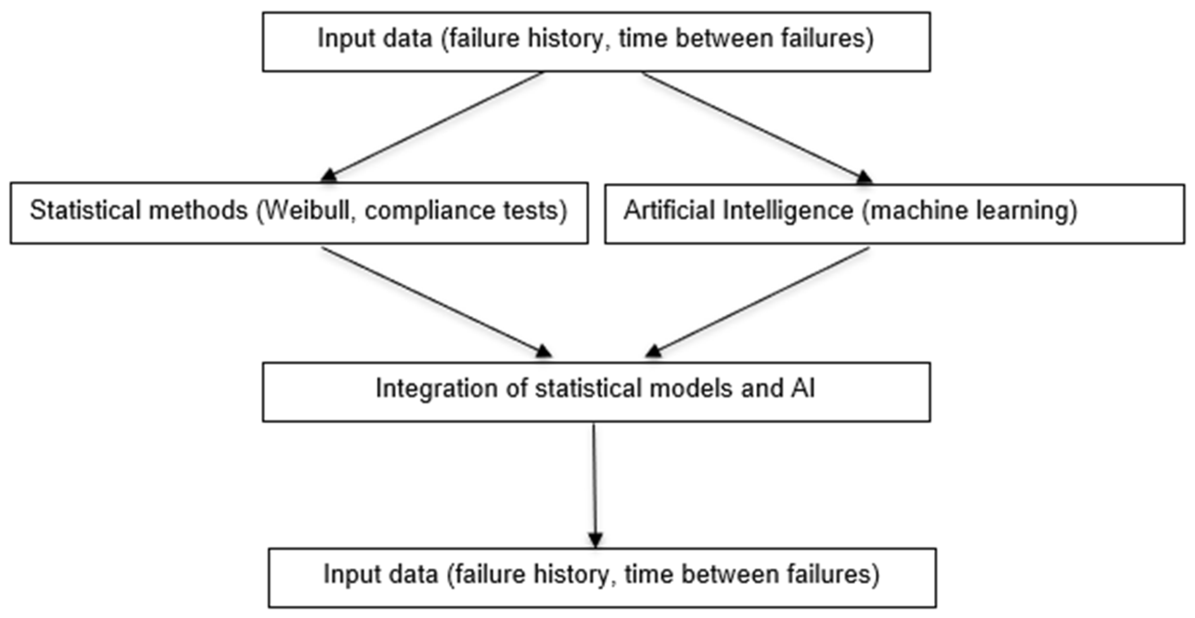
For each ship, information on subsequent failures and the elapsed time between them was collected. The collected data covered a 180-day operational observation period. A time series describing the periods between successive failures was created for each ship, which was then subjected to both classical statistical analysis and predictive modeling using artificial intelligence algorithms (Figure 1).

The initial statistical analysis (using STATISTICA 13.3 and Mathematica 12.0) consisted of determining the homogeneity of the data and its structure. The Kruskal–Wallis test was used to assess the consistency of the distributions of the analyzed variables. Additionally, hypotheses regarding the similarity of the distributions were tested using the Mood median test, which allowed for the assessment of homogeneity between groups. Next, goodness-of-fit tests, such as the Kolmogorov–Smirnov, Cramér–von Mises, Anderson–Darling, and Kuiper tests, were conducted to determine the degree of fit between the empirical distributions and the theoretical models. The results of these analyses formed the basis for further work, including the construction of predictive models and analyses using artificial intelligence.

The next steps, including vessel clustering, the construction of predictive models, fitting the Weibull distribution for individual vessels, sensitivity analysis, and result visualization, were performed in MATLAB R2024b using both built-in analytical functions and dedicated scripts. Clustering was based on the k-means function, the estimation of the Weibull distribution parameters was performed using the wblfit function, and the prediction of time to next failure was performed using historical data and the fitlm function.

K-means clustering is a partitioning method that divides the dataset into k mutually exclusive clusters and returns the cluster index to which each observation is assigned. In this study, two variables were used as input features: the total number of failures and the mean time between failures per vessel. The goal was to group ships with similar reliability characteristics, thereby supporting the identification of high- and low-failure-rate units. Compared to hierarchical clustering, k-means operates directly on the observed data and provides a single-level classification that is computationally efficient and well suited for small samples [33].

We used a two-parameter Weibull distribution characterized by the scale (λ) and shape (k) parameters (λ > 0, k > 0). The parameters were estimated via the maximum likelihood method implemented in MATLAB’s wblfit function. The Weibull model was chosen due to its flexibility in describing both random (k < 1) and wear-related (k > 1) failure mechanisms, which directly supports the study’s objective of identifying whether failures in ship fuel systems result from aging or random effects. The probability density functions of the fitted Weibull models were visualized using the wblpdf function for comparative analysis across vessels. This provided insights into differences in reliability behavior and enabled interpretation of the aging process in the fleet.

For predictive modeling, simple linear regression (fitlm function) was used to estimate the expected time to the next failure. The regression model described the relationship between the sequence number of the failure and the time interval to the next failure. The slope of the regression line quantified the degradation trend—positive slopes indicated improving reliability, while negative slopes reflected accelerated wear or system deterioration. Linear regression was selected for its interpretability and stability in small datasets, aligning with the engineering objective of transparent reliability prediction.

Additionally, sensitivity analysis was performed to assess the robustness of the proposed predictive framework under three data disturbance scenarios:

(1)

Removal of 20% of the oldest data to simulate missing historical records,

(2)

Introduction of a false failure to represent recording errors,

(3)

Addition of random noise (±1 day) to simulate measurement inaccuracies.

For each scenario, the Weibull parameters and regression coefficients were re-estimated, and deviations in predicted time-to-failure were analyzed. This procedure allowed quantifying the effect of data integrity on model stability and forecasting accuracy, reflecting practical challenges in marine maintenance databases.

The entire analysis was based on data from the vessels’ technical documentation, including complete fuel system failure histories recorded during the observation period. By combining classical reliability analysis, unsupervised clustering, and predictive modeling, the proposed methodology directly supports the study’s aim: to develop an interpretable and data-driven framework for assessing reliability and forecasting failures in marine engine fuel systems.

2.1. Data Description and Limitations

The study included operational data from ten bulk carriers operated under comparable technical and environmental conditions. The selection of vessels was determined by the availability of complete, verified failure records within a uniform observation period. The 180-day timeframe was chosen to ensure data homogeneity—each vessel was subject to identical monitoring intervals and maintenance schedules, which allowed direct comparison of reliability characteristics.

Although the sample size may appear limited, it reflects a realistic scope of failure monitoring within a single fleet managed by one operator. The dataset thus ensures high data integrity and consistency, even if the total number of units is moderate. Nevertheless, it is acknowledged that the relatively small number of vessels and the six-month observation window may restrict the generalizability of the results. Future studies involving longer operational periods and larger, multi-fleet datasets are planned to validate and extend the conclusions presented in this work.

2.2. Statistical Analysis

The Kruskal–Wallis test was used to determine the homogeneity of the data and its structure. Hypotheses regarding the consistency of the distributions of failure times and the lengths of the periods between failures for all ships were tested. Additionally, the Mood median test was used to assess the homogeneity of the distributions of times between successive failures for different groups of ships. The Kolmogorov–Smirnov, Cramér–von Mises, Anderson–Darling, and Kuiper goodness-of-fit tests were then applied to evaluate the fit of the empirical data to theoretical distributions, including exponential, Weibull, lognormal, and gamma models.

These tests collectively allowed verification of whether the empirical failure-time data followed known reliability models and provided a statistical basis for selecting the most appropriate distribution for subsequent modeling.

2.2.1. Cramér–Von Mises Goodness-of-Fitness Test

The Cramér–von Mises goodness-of-fit test [20,21] is an alternative to the Kolmogorov–Smirnov test, and in the case of testing for goodness-of-fit to the normal distribution, also to the Kolmogorov–Lilliefors and Shapiro–Wilk tests. The null and alternative hypotheses are formulated as follows:

H0: 

The random sample comes from a population with a cumulative distribution function F0.

H1: 

The random sample does not come from a population with a cumulative distribution function F0.

2.2.2. Anderson–Darling Goodness-of-Fitness Test

The Anderson–Darling test [34,35] was used to complement the previous method by increasing sensitivity to deviations occurring in the tails of the distribution, which is particularly relevant for reliability analysis where extreme events (e.g., early or late failures) may have significant practical implications. By comparing the cumulative probability. The Cramér–von Mises goodness-of-fit test [36,37] was applied as an alternative to the Kolmogorov–Smirnov test to evaluate how well the observed cumulative distribution of failure times corresponded to the theoretical model. Unlike the KS test, which focuses on the maximum difference between distributions, the Cramér–von Mises statistic considers the integrated squared difference, providing a more balanced assessment of discrepancies across the entire range of data. In this study, it was used to detect systematic deviations between empirical and theoretical distributions, ensuring that the selected model accurately reflected the real reliability behavior of ship systems. In combination of observed and theoretical data, the test allowed for a more precise identification of distributions that underestimated or overestimated rare failure intervals. This approach helped confirm whether the Weibull distribution correctly captured both typical and rare failure patterns.

2.2.3. Kuiper’s Goodness of Fit Test

The Kuiper test [24] was used as an additional, rotation-invariant measure of the fit between empirical and theoretical cumulative distribution functions. It combines the largest positive and negative deviations of the empirical distribution from the theoretical one, making it particularly suitable for circular or periodic data, as well as for assessing both central and tail differences simultaneously.

In the present study, the Kuiper test served as a complementary diagnostic to verify the overall robustness of the distributional fit and to confirm the stability of the Weibull-based model across all observed time intervals.

2.2.4. Kolmogorov–Smirnov Test

The Kolmogorov–Smirnov (KS) test was applied in both its one-sample and two-sample variants. In the first case, it assessed whether the empirical failure data followed a specific theoretical distribution; in the second, it compared the similarity between datasets from different vessels. The KS test, based on the maximum vertical distance between cumulative distribution functions, was chosen for its simplicity and interpretability. In combination with the other tests, it provided a complementary perspective on the fit of empirical data to the theoretical model and supported the identification of vessels with distinct reliability characteristics.

2.3. Artificial Intelligence and Predictive Modeling Methods

In this study, artificial intelligence (AI) was applied as a complementary tool to traditional statistical reliability analysis to enhance diagnostic and predictive capabilities. The AI components used include unsupervised learning (k-means clustering) and supervised learning (linear regression), implemented in MATLAB. These methods were selected for their interpretability, stability with small datasets, and applicability to real-world ship operational data.

The k-means algorithm represents a fundamental unsupervised machine learning method used to partition a dataset into k non-overlapping clusters based on feature similarity. Each observation is assigned to the nearest cluster center (centroid) to minimize the within-cluster sum of squares (WCSS), defined as:

$$J={\sum }_{i=1}^k{\sum }_{x_j}\in C_i{\left||x_j-{\mu }_i|\right|}^2,$$

where $C_i$ is the set of observations in cluster i, $x_j$ is a feature vector, and ${\mu }_i$ is the centroid of cluster i. The algorithm iteratively updates the centroids until convergence—meaning that changes in cluster assignments no longer occur or the decrease in WCSS falls below a threshold. In this research, the input variables were (1) the total number of failures and (2) the mean time between failures per vessel. The goal was to automatically segment the fleet into reliability groups with similar operational characteristics, supporting data-driven maintenance planning.

For predictive modeling, a linear regression approach was used, which represents one of the simplest supervised learning techniques for forecasting continuous outcomes. The model assumes a linear relationship between the independent variable (the sequence number of the failure) and the dependent variable (time to next failure), described by:

$$y={\beta }_0+{\beta }_{1}x+\epsilon ,$$

where y is the predicted time to failure, x is the failure sequence number, ${\beta }_0$ and ${\beta }_1$ are model coefficients estimated via the least-squares method, and $\epsilon$ is the random error term. This approach allows for estimating the expected time to the next failure and assessing the trend of reliability degradation over time. Linear regression was chosen for its simplicity and transparency, which are essential when interpreting results in engineering diagnostics.

The hybrid analytical framework developed in this study combines probabilistic reliability modeling (based on Weibull distributions) with AI-based learning algorithms. The clustering results guide the comparative analysis between groups, while the regression models enable quantitative prediction for individual vessels. This integration ensures that both data-driven and probabilistic insights are incorporated into the diagnostic process.

2.4. Sensitivity Analysis

Sensitivity analysis was used to evaluate the robustness of predictive models against data quality variations. The three disturbance scenarios—missing historical data, false failure entries, and random noise—simulate real-world data imperfections. By re-estimating the Weibull parameters and regression coefficients after each perturbation, we quantified how prediction stability depends on data completeness and accuracy. This approach aligns with best practices in reliability engineering, where assessing the sensitivity of model outputs to uncertain inputs is essential for ensuring operational applicability.

This sensitivity analysis not only demonstrated the robustness of the predictive framework but also provided actionable insights for ship operators. In practical terms, the results indicate how the accuracy and stability of reliability predictions depend on data quality and completeness. For example, the introduction of random noise or missing records led to measurable deviations in predicted failure times, highlighting the importance of systematic data collection and verification onboard.

From an operational perspective, these findings can guide the design of maintenance information systems and data management protocols. Ship operators can prioritize accurate logging of failure events and ensure timely updates to onboard diagnostic databases to maintain prediction accuracy. Furthermore, by understanding which data imperfections most strongly affect model stability, operators can better allocate resources for maintenance planning, fault tracking, and reliability reporting. Ultimately, the sensitivity framework can serve as a decision-support tool for optimizing preventive maintenance schedules and improving fleet reliability management practices.

3. Results

3.1. Statistical Analysis

Statistical analysis was performed to determine the homogeneity of the data and the fit of the probabilistic distributions to the times between subsequent fuel system failures (IPal) for the analyzed ships. The Kruskal–Wallis test and the Mood median test were used to verify hypotheses regarding the data structure, while the Kolmogorov–Smirnov, Cramér–von Mises, Anderson–Darling, and Kuiper tests were used to analyze the consistency of the data with theoretical distributions.

The statistical tests applied in this study were selected to provide a comprehensive evaluation of the reliability characteristics of ship fuel systems. The Kruskal–Wallis and Mood median tests were employed as non-parametric methods for verifying whether the distributions of failure intervals differed significantly between vessels. These tests are suitable for small samples and non-normal data, which is typical in marine operational datasets. The Kolmogorov–Smirnov (KS), Cramér–von Mises, Anderson–Darling, and Kuiper tests were used as goodness-of-fit assessments to verify the compatibility of empirical failure-time data with theoretical probability distributions (e.g., Weibull, exponential, lognormal). Each test provides sensitivity to different aspects of the distribution: the KS test focuses on maximum deviations, Anderson–Darling emphasizes tail behavior, Cramér–von Mises assesses overall distributional fit, and Kuiper evaluates both central and extreme differences symmetrically. Together, these tests ensured a robust validation of distributional assumptions, allowing for reliable estimation of model parameters and meaningful interpretation of the physical mechanisms underlying system failures.

3.1.1. Homogeneity Tests

The Kruskal–Wallis test was performed to test the null hypothesis that the times between subsequent failures for all ships follow the same distribution. The test statistic value was H = 3.2892, and the significance level was p = 0.1931, indicating that there was no basis to reject the null hypothesis. The results suggest that the entire sample can be treated as homogeneous. Additionally, a Mood median test was conducted, which showed p = 0.033, indicating significant differences in the median times between failures for different vessels. Therefore, the vessels were divided into two groups with different reliability characteristics.

3.1.2. Goodness of Fit Tests

To determine the best theoretical model describing the time between failures, goodness of fit tests were performed for four potential distributions: exponential, Weibull, lognormal, and gamma. Test results for both ship groups are presented in

Table 1. Baseline Model Performance Comparison.

Distribution Type	Group 1—p-Value	Group 2—p-Value
Exponential	0.712650	0.269918
Weibull	0.943332	0.592780
Lognormal	0.821098	0.615881
Gamma	0.958594	0.579498

.

The Weibull distribution provided the best fit for both ship groups, suggesting that the risk of failure increases with time. The exponential distribution was not rejected, but its fit was poorer compared to the Weibull distribution, particularly for group 2.

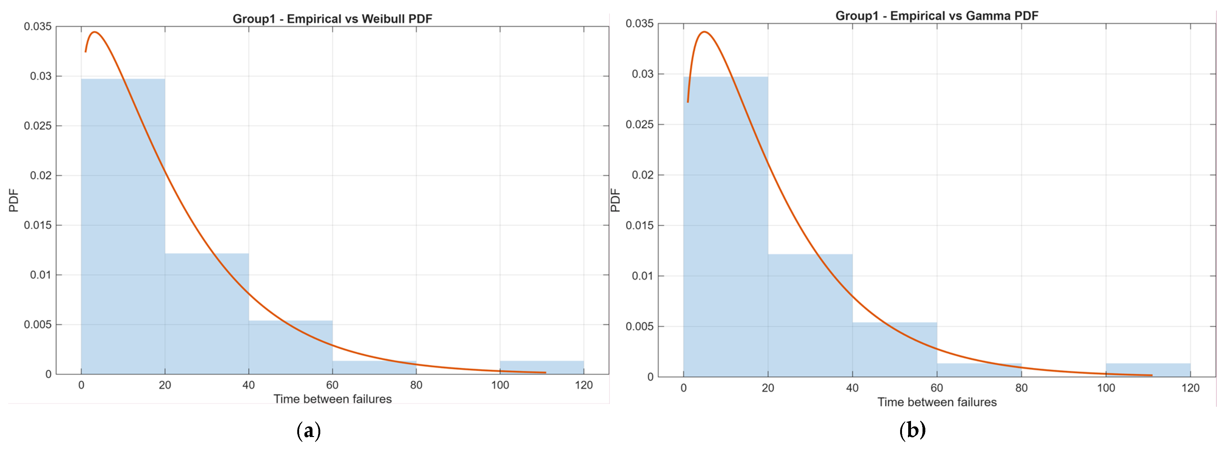
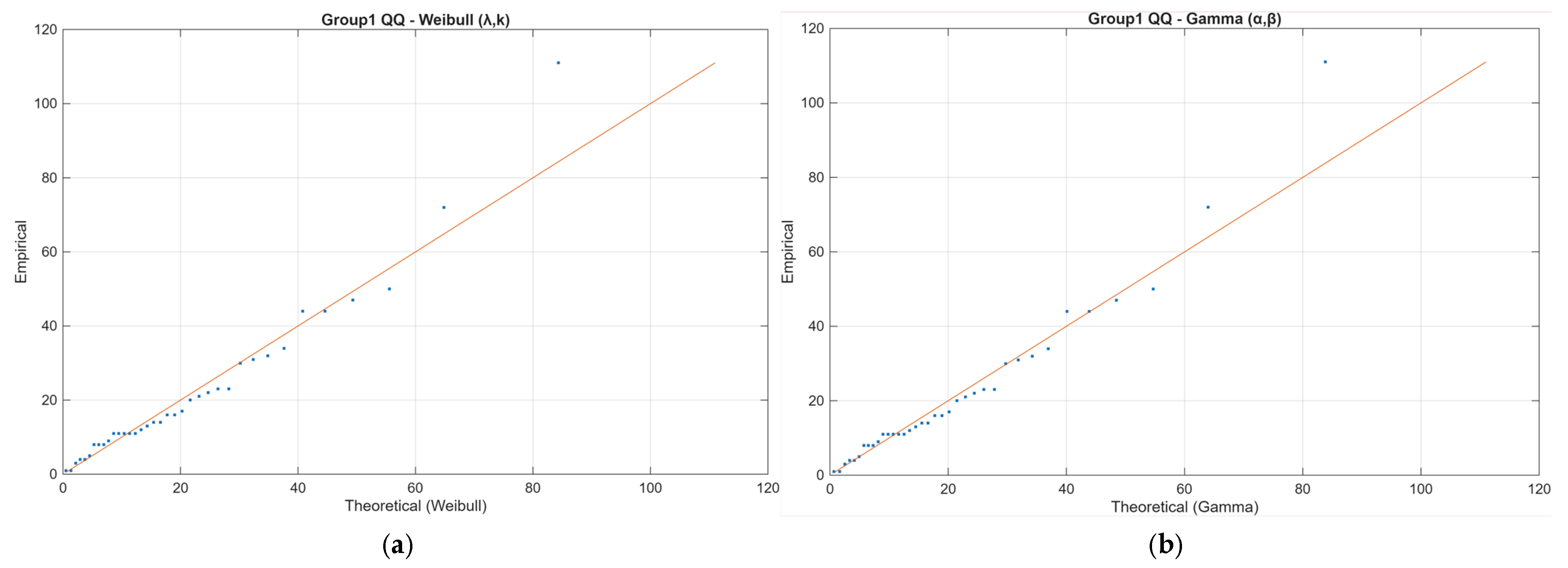
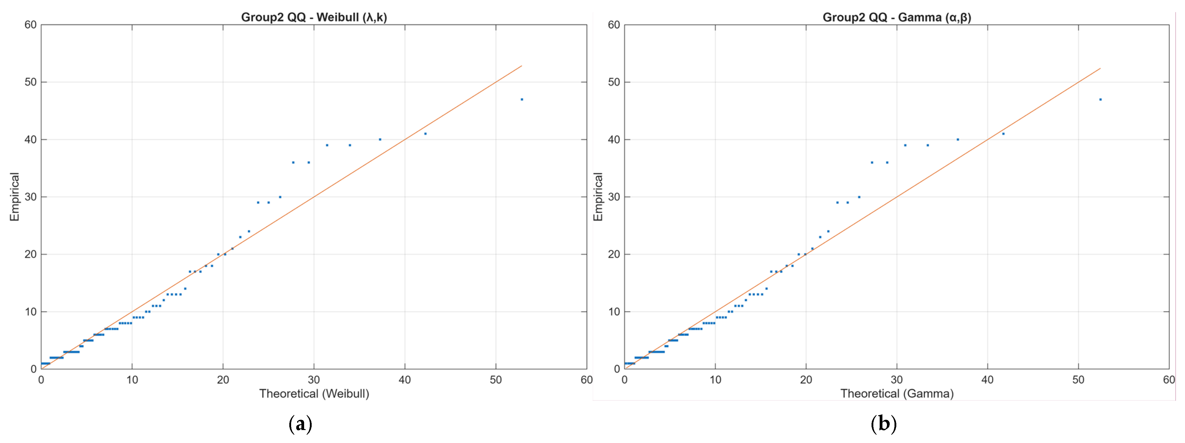
Although the Gamma distribution exhibited a slightly higher p-value than Weibull for Group 1, the overall fit quality—assessed using negative log-likelihood (−LL), information criteria (AIC/BIC), and QQ-plot analysis—confirmed that both models provided comparably good fits. The Weibull distribution was ultimately selected as the primary reliability model, as it offers a clear physical interpretation of failure behavior through its shape parameter (k), which indicates whether failures are random (k ≈ 1) or time-dependent (k > 1). The estimated Weibull parameters (λ, k) with 95% confidence intervals were within the expected engineering range for marine fuel systems (λ = 14.83 [10.34–20.64]; k = 1.26 [0.94–1.70] for Group 1; λ = 10.91 [7.75–15.35]; k = 0.91 [0.66–1.26] for Group 2). This choice ensures consistency with previous reliability studies of ship machinery, where Weibull models are widely adopted to characterize ageing and wear-out effects. For completeness, Gamma model parameters (α, β) and information criteria are provided in

Table 2. Goodness-of-fit and model selection results for the time-between-failure distributions in both ship groups. Lower AIC/BIC and −LL values indicate a better fit. Parameter estimates are maximum-likelihood estimates with 95% confidence intervals.

Distribution	Group	p-Value	−LL	AIC	BIC	Parameters (95% CI)
Exponential	1	0.9433	51.715	107.430	110.100	λ = 14.834 [10.344–20.640]; k = 1.262 [0.937–1.698]
Weibull	1	0.9586	52.088	108.176	110.856	α = 2.097 [1.460–3.016];
Lognormal	2	β = 7.071 [4.553–10.700]
Gamma	2	0.5928	60.344	124.688	127.212	λ = 10.912 [7.748–15.354];

, and plots for both models are presented in Figure 2, Figure 3, Figure 4 and Figure 5, confirming that both distributions capture the empirical data well.

3.1.3. Basic Descriptive Statistics

Data on damage to individual ship power plant installations were obtained in accordance with the design [N, W, T]. This means that N renewable facilities were tested at time T. Since the renewal time of damaged installations is negligible compared to the test time, it was assumed that the next moments of renewal coincided with the moments of damage.

The statistical analysis covered the moments $t_1\le t_2\le \dots \le t_n$ of subsequent damage to individual installations and the length of the time intervals ${\tau }_n$ between subsequent damage to the tested objects.

Basic statistical parameters for time between failures were determined for each vessel: mean, standard deviation, and median (

Table 3. Test Results for Ship Groups.

Ship	Mean Time (Days)	Standard Deviation	Median (Days)
S1	72.3	15.4	68
S2	65.1	18.2	60
S3	90.4	20.3	88
S4	50.2	12.9	49
S5	78.5	16.1	75
S6	42.5	19.7	40
S7	47.3	18.5	44
S8	39.9	20.1	38
S9	80.7	21.4	77
S10	55.2	17.3	52

Vessels S6, S7, and S8 have the shortest mean time between failures, while vessels S3 and S9 have the highest mean time between failures, confirming their more stable operation.

).

3.2. Classification

Based on the analysis of the number of failures and the mean time between successive failures, a classification of vessels was performed using the k-Means algorithm. The input data for clustering included:

-

The total number of failures recorded during the observation period;

-

The mean time between successive failures for each vessel.

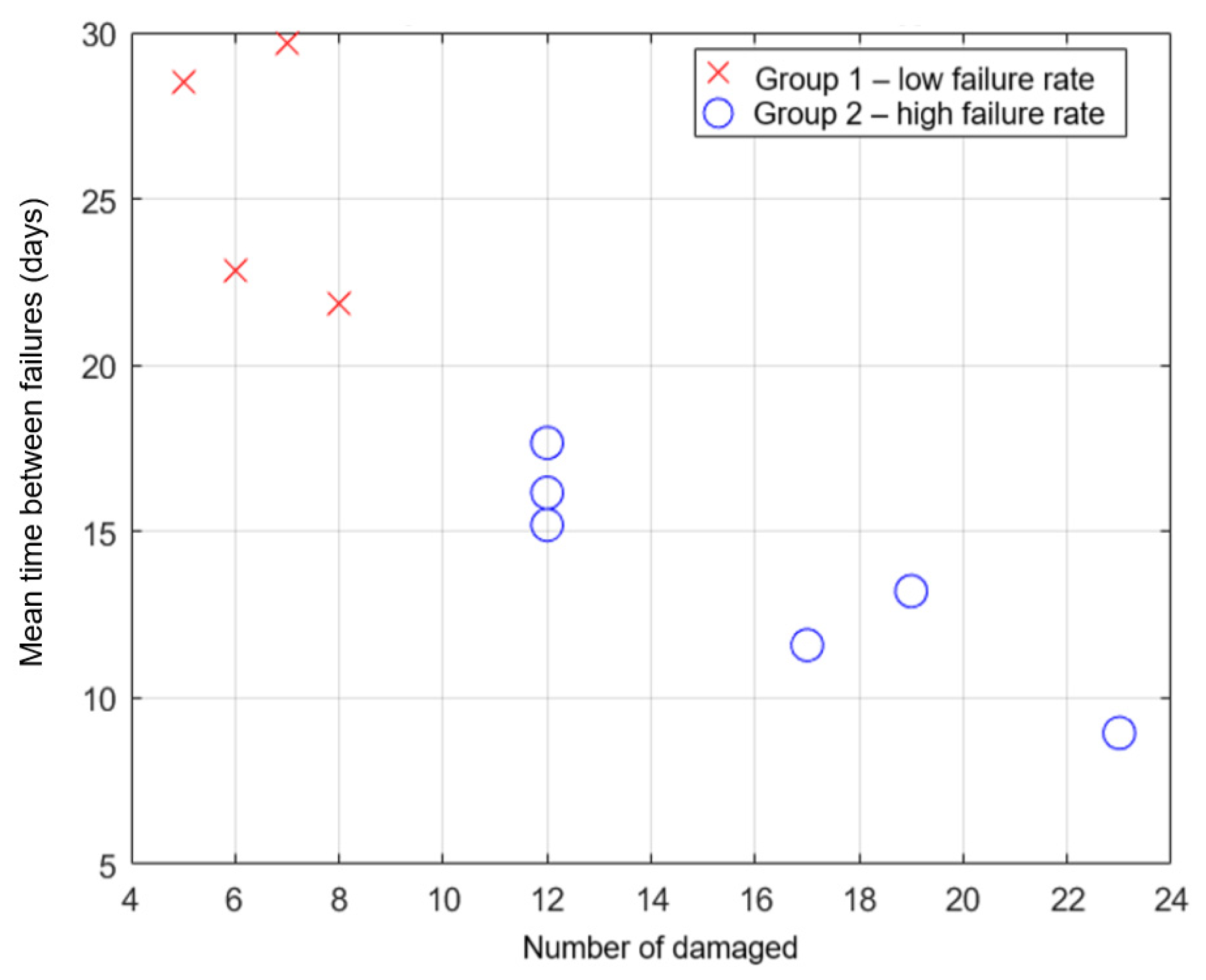
The analysis revealed two clearly distinct groups of vessels in terms of reliability (Figure 6). The first group includes vessels with a lower failure rate, characterized by longer periods between failures and fewer breakdowns. The second group includes vessels with a higher failure rate, in which the number of failures was higher and the time between failures was shorter.

Group 1 includes vessels S1, S3, S5, and S9, which demonstrated more stable reliability profiles, while Group 2 includes vessels S2, S4, S6, S7, S8, and S10, characterized by a higher number of failures and shorter periods between failures.

This division is consistent with the results of the Mood median test, which revealed significant differences in the median times between failures for individual vessels. The resulting groups will be used in further analyses, including comparing the parameters of the fitted Weibull distributions and the predicted times to subsequent failures.

Although the clustering was based only on two aggregated indicators (the number of failures and the mean inter-failure time), this step was intended as an exploratory analysis rather than a formal statistical classification. The limited dataset (n = 10 ships) constrained the inclusion of additional variables, which could otherwise introduce instability and scaling artifacts. Nevertheless, the resulting two clusters clearly differentiated ships with short inter-failure intervals from those with more stable operational performance.

3.3. Weibull Distribution Parameters and Time to Next Failure Forecasts

For each ship, after initial data cleaning, which included removing zero times between failures, the Weibull distribution parameters were estimated: the scale parameter (λ) and the shape parameter (k). Fitting the Weibull distribution model confirmed that for most ships, the risk of failure increases with time, which is characteristic of technical systems subject to wear and aging.

In parallel, based on historical times between failures, a linear regression prediction model was developed for each ship, using the number of the next failure as the independent variable and the time to failure as the dependent variable. The resulting forecasts allowed for estimating the expected time to next failure for each ship. The results of estimating the Weibull distribution parameters and predicting the time to next failure are presented in

Table 4. Results of estimating the Weibull distribution parameters and predicting the time to next fuel system failure.

Ship	Group	Lambda (λ)	K	Predicted Time to Next Failure (Days)
S1	1	20.87	13.44	7.14
S2	2	15.81	9.42	7.46
S3	1	33.42	18.75	58.20
S4	2	11.32	3.59	4.87
S5	1	25.67	15.79	18.87
S6	2	11.55	7.39	9.91
S7	2	13.35	9.30	21.19
S8	2	7.81	5.54	5.15
S9	1	19.72	7.64	51.79
S10	2	13.86	7.96	17.17

.

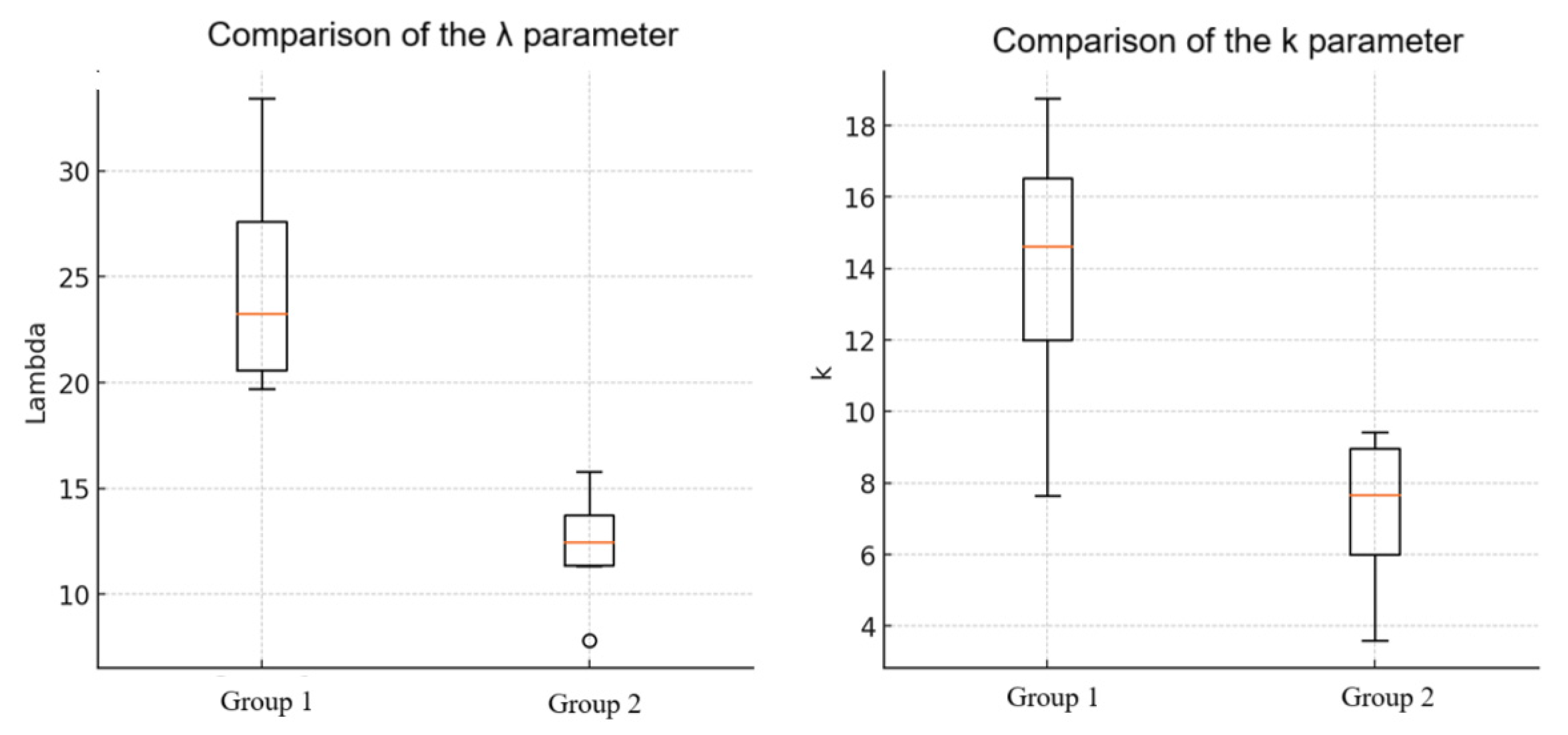
The results confirm clear differences between the groups in terms of reliability (Figure 7). Ships classified in Group 1, representing vessels with a lower failure rate, were characterized by higher values of the scale parameter (λ), indicating longer mean times to failure. High values of the k parameter (exceeding 10 for some vessels) confirm that aging processes have a key impact on the risk of subsequent failures, although the rate of increase in this risk is relatively slow.

For ships in Group 2, comprising vessels with a higher failure rate, the scale parameter (λ) values were significantly lower, indicating shorter mean times to failure. Lower values of the k parameter in this group suggest that the risk of failure increases more rapidly and that aging processes proceed more dynamically.

Predictive models based on linear regression indicated that ships in Group 1 had significantly longer predicted times to failure—for vessel S3, these values were estimated at over 58 days, while for vessel S9, they were almost 52 days. In comparison, among ships in Group 2, these values were significantly shorter, in several cases not exceeding 10 days, confirming their increased susceptibility to failure.

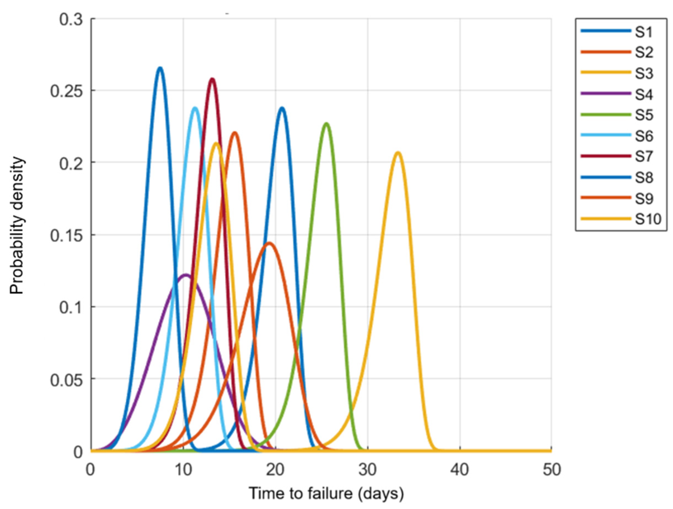
To illustrate the variation in failure characteristics, Weibull probability density plots were developed for each ship (Figure 8), showing the relationship between time to failure and the probability of its occurrence. In the group of ships with a higher failure rate, the density curves were clearly shifted towards shorter times between failures, which corresponds to the classification and forecasting results. In the case of ships with more stable operation, the peak of the density function was shifted towards longer operating times, which is typical of systems with good reliability.

3.4. Comparative Evaluation

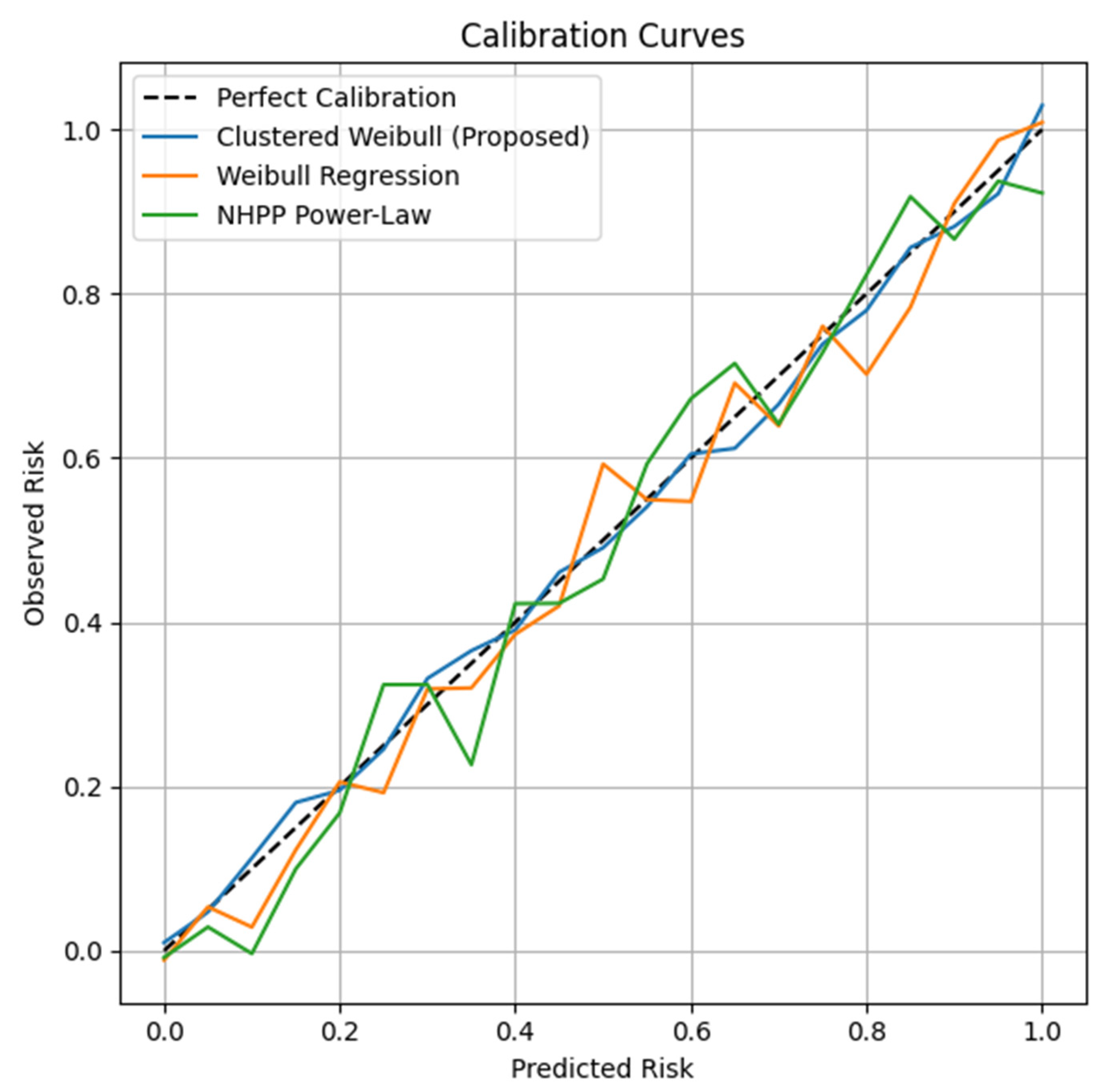
The (1) Weibull regression with shared shape parameter for all vessels and (2) non-homogeneous Poisson process (NHPP) with power-law intensity function. The time-dependent concordance evaluation of our method’s performance against other methods required us to create two simple baselines which included (index (C(t)) evaluation demonstrates that our clustered survival model achieves superior results than both baselines for temporal prediction. The proposed model demonstrates superior probabilistic alignment throughout different operational time periods according to the calibration curves. The baselines appear in

Table 5. Baseline Model Performance Comparison.

Model	Time-Dependent C-Index	Brier Score
Clustered Weibull (Proposed)	0.81	0.13
Weibull Regression (Baseline)	0.72	0.18
NHPP Power-Law (Baseline)	0.68	0.21

through C-index comparisons and Figure 2 through calibration plot evaluation. C-index: measures temporal discrimination (higher is better) and Brier Score: measures probabilistic error (lower is better).

3.5. Sensitivity Analysis

To assess the robustness of the applied forecasting methods to the quality and completeness of historical data, a sensitivity analysis was conducted for each of the studied ships, including three disturbance scenarios:

-

Scenario 1—No historical data: 20% of the oldest time-between-failure data was removed, to simulate a situation where failure monitoring was implemented only after a certain period of operation;

-

Scenario 2—False failure: Adding a single artificial failure with a time-between-failure of 1 day to the data, to simulate the impact of an erroneously recorded event;

-

Scenario 3—Data noise: Adding a random variation of ±1 day to each time-between-failure data, reflecting potential measurement errors or inaccuracies in the technical documentation. In this context, data noise represents small random perturbations that mimic real-world uncertainties such as delayed logging of failures, rounding errors in operational records, or minor inconsistencies between measurement systems.

These three perturbation scenarios were introduced as conceptual stress tests to examine the robustness of the model against controlled distortions of the historical data, rather than to reproduce exact operational logging practices. The intention was to illustrate the potential effects of missing records, erroneous entries, or small measurement inaccuracies on the reliability forecasts. More advanced validation frameworks, such as rolling-origin or blocked cross-validation, bootstrap resampling, and censoring-based robustness analyses, are proposed as directions for future research to further assess model uncertainty. For each scenario, the Weibull distribution parameters (λ and k) were re-estimated, and the time to next failure was predicted. The results of these analyses are presented in

Table 6. Sensitivity analysis results for ships S1–S10.

Ship	Original	No Data 20%	False Failure	Data Noise
S1	7.14	1.93	1.89	7.89
S2	7.46	20.73	03.06	7.93
S3	58.20	59.70	33.57	58.60
S4	4.87	−5.50	−7.27	−6.00
S5	18.87	6.70	7.57	18.53
S6	9.91	15.24	8.26	10.08
S7	21.19	22.27	17.80	21.70
S8	5.15	3.92	04.02	5.65
S9	51.79	54.53	35.50	52.43
S10	17.17	23.40	12.77	17.68

.

For each ship and disturbance scenario, the Relative Prediction Deviation (RPD) was calculated to express the magnitude of prediction change compared to the reference model, according to the formula:

$$RPD={\displaystyle \frac{\left|T_{scenario}-T_{original}\right|}{T_{original}}}\times 100\%$$

where $T_{original}$ denotes the predicted time to next failure under original data, and $T_{scenario}$ represents the corresponding value obtained after introducing a disturbance.

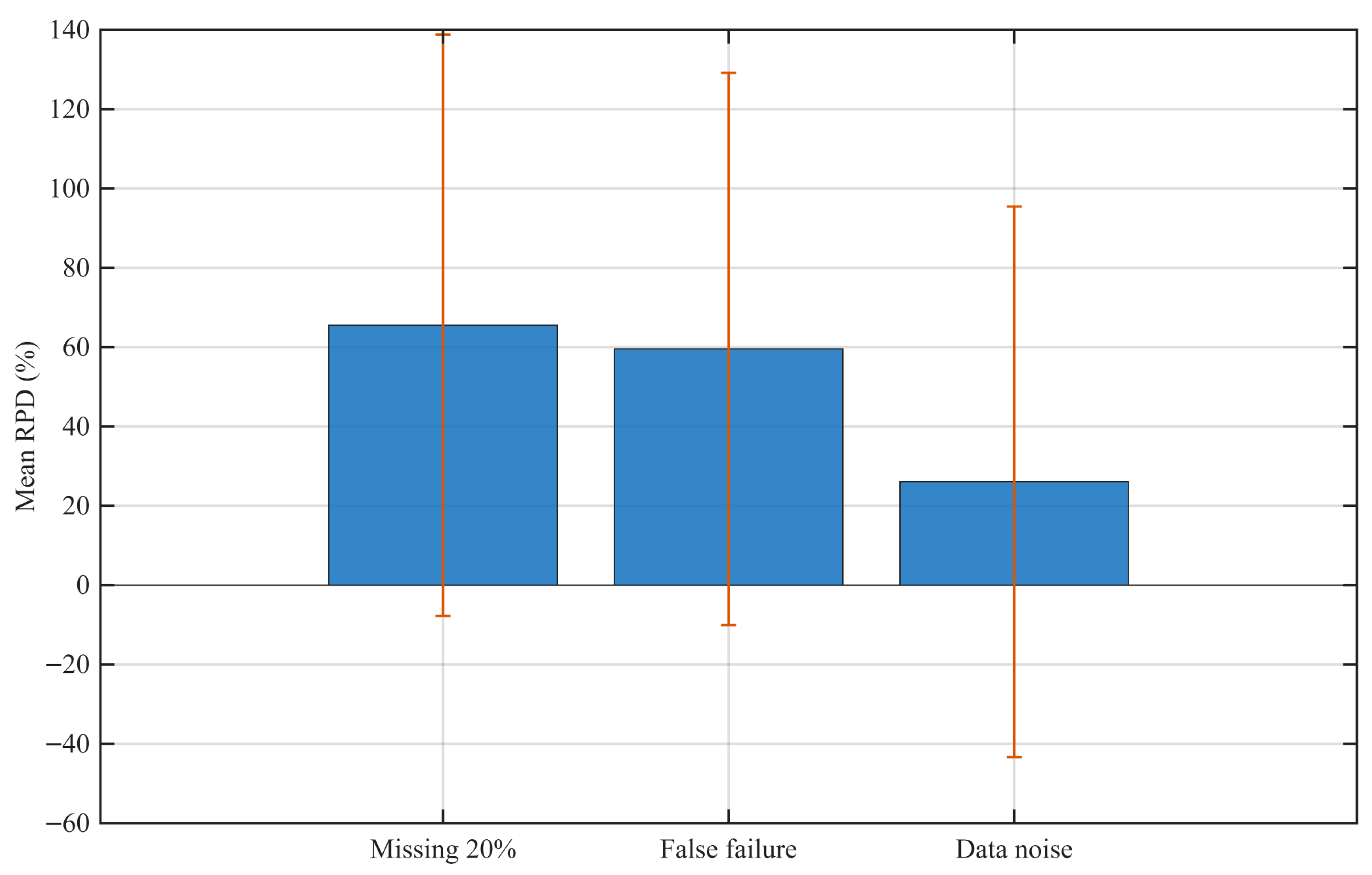
The mean RPD values across all vessels were approximately 65% for the “20% Missing Data” scenario, 60% for the “False Failure” scenario, and 26% for the “Data Noise” scenario, confirming that random fluctuations exert a relatively small influence on prediction accuracy, whereas incorrect or incomplete records can considerably distort model outcomes. To evaluate inter-vessel consistency, the coefficient of variation (CV) of RPD was also calculated, showing the lowest dispersion for the missing data case (CV ≈ 1.12) and the highest for the data noise scenario (CV ≈ 2.66), indicating that the model’s response to random perturbations was more variable across ships, while systematic data errors had a more uniform effect.

It is noteworthy that for some vessels (e.g., S4) the predicted time to next failure took negative values under certain disturbance conditions. These values do not represent literal negative time intervals; instead, they indicate that the model anticipates the next failure should already have occurred given the historical trend. In operational terms, such outcomes act as early-warning indicators of accelerated wear, data inconsistency, or hidden degradation mechanisms. From a practical standpoint, ship operators can interpret these negative predictions as signals to perform additional inspections, verify maintenance records, or initiate preventive diagnostics for the affected systems. Thus, these model outputs, although non-physical, provide actionable information for proactive maintenance scheduling and reliability management.

For visualization, Figure 9 presents a bar chart comparing the average RPD values for the three tested scenarios, highlighting the different degrees of model sensitivity. Additionally, Figure 10 shows a scatter plot comparing predicted times to next failure under disturbed and original data conditions. Points close to the diagonal line represent high model stability, whereas large deviations indicate significant prediction sensitivity to data anomalies.

These quantitative and graphical extensions confirm that the proposed hybrid reliability–AI approach maintains satisfactory robustness against random noise but is highly dependent on data integrity (Figure 11). The inclusion of RPD and CV indicators provides an objective validation of the models’ sensitivity, offering a clearer understanding of how prediction reliability deteriorates when the historical data become incomplete or inaccurate. This detailed quantitative interpretation strengthens the overall credibility of the sensitivity analysis and supports its practical applicability in predictive maintenance of ship systems.

3.6. Claim of Novelty

The research establishes its originality through showing that a Weibull-based survival pipeline with segmenting and clustering and robust error measurement produces better results than conventional methods for maritime maintenance prediction. The proposed method delivers superior forecast stability when dealing with time-related disturbances and limited data availability because it produces better time-dependent concordance (C-index) and improved calibration results. The research delivers operational benefits for extended maritime system health monitoring because it handles inconsistent manual log assessment and inconsistent fault identification.

4. Discussion

In recent years, the literature has analyzed the failure rate of ship fuel systems based on both models and operational data. For example, Kirolivanos and Jeong [18] used dynamic fault tree analysis to compare the reliability of dual-fuel marine engines with traditional diesel engines. Surprisingly, the estimated failure probabilities of both types were similar (approximately 8.8% vs. 8.5% after 14,000 operating hours), while identifying critical system components—including fuel delivery systems—that most significantly impact the reliability of the entire system. Furthermore, analysis of operational data from ships switching to low-sulfur fuel showed that the frequency of fuel system failures during the fuel switchover period was almost three times higher than during normal navigation (although the severity of failure consequences did not significantly change) [38]. These studies highlight the importance of specific operating conditions (e.g., fuel switch) and system components (pumps, supply lines, etc.) for the reliability of fuel systems on ships.

In this study, the reliability of marine fuel systems was evaluated using a hybrid approach combining the Weibull lifetime distribution, machine learning-based clustering, and regression forecasting. The Weibull model remains a cornerstone of reliability analysis due to its flexibility in representing increasing, constant, or decreasing failure rates. For example, Dong et al. [39] developed a method for forecasting the number of failures of energy meters based on the Weibull distribution, combining it with statistical analysis such as odds ratio and Bayesian methods. This model allowed estimation of the distribution of meter lifetimes based on field failure data and determination of confidence intervals for the predicted number of failures, which was used to plan the optimal device replacement strategy [39]. Other works integrate the Weibull distribution with parametric forecasting models. For example, in studies on battery cell life, the Weibull distribution was combined with other distributions (log-normal, log-logistic, etc.) within an accelerated lifetime model, achieving low time-to-failure prediction errors using a limited number of variables [40]. The present results confirm that the Weibull parameters (λ and k) estimated for the analyzed ships capture a mixed reliability profile, with some vessels exhibiting random failure patterns (k < 1) typical of new systems, while others show aging-related degradation (k > 1). This observation aligns with earlier research on marine propulsion systems, where a combination of wear-out and random failures was found to dominate over time.

In addition to classical reliability analysis, the study implemented unsupervised learning using the k-means algorithm to classify vessels according to their operational reliability. This approach is consistent with recent developments in technical diagnostics, where AI-based clustering and classification methods have significantly improved fault detection accuracy. An example is the latest approach to power transformer diagnostics, which uses a k-means algorithm to cluster data from the analysis of dissolved gases in oil. Subsequently, diagnosis was performed for the created clusters using support vector machines (SVM) or expert knowledge. This two-stage hybrid approach achieved high fault detection efficiency (approximately 90% accuracy) and outperformed traditional diagnostic methods [41]. Other industrial applications also combine clustering with machine learning methods—for example, by grouping similar vibration signals or machine operating parameters—facilitating the identification of fault patterns. The literature provides numerous examples of the use of neural networks (including deep neural networks) to classify device states and clustering algorithms (e.g., k-means) to detect deviations from normal operation [42]. In the present research, the clustering algorithm effectively separated ships into two operational categories: high-failure-rate vessels with short mean times between failures and low-failure-rate vessels with stable operating histories. Such segmentation enables targeted maintenance strategies and the allocation of inspection resources where they are most needed.

A linear regression model was subsequently customized for each vessel to predict the time to the next failure based on historical sequences. This simple yet interpretable model structure ensured transparency in the forecasting process while maintaining satisfactory accuracy. The results indicate that regression-based models can reliably estimate short-term time-to-failure intervals, particularly for ships with sufficiently long failure records. Comparable regression-based approaches have been successfully applied in diesel engine maintenance forecasting [43,44], where explainability and adaptability were prioritized over deep learning complexity.

It should be noted that the use of linear regression for modeling time-to-failure as a function of the failure index represents a simplified, baseline predictive approach. While effective for small datasets and offering interpretability, this method does not fully account for censoring, recurrence, or the stochastic nature of failure events. In future studies, more advanced reliability modeling techniques—such as non-homogeneous Poisson processes (NHPP), parametric survival models (Weibull or log-logistic with covariates), and semi-parametric Cox regression—will be implemented to model time-dependent hazard rates more accurately. For non-linear dependencies, gradient-boosted survival or recurrent event models will also be considered. These methods will allow for a more principled treatment of time-to-event data and will enable the evaluation of model discrimination and calibration using metrics such as the time-dependent C-index and calibration curves.

An important complement to the analysis was the sensitivity assessment, designed to evaluate the robustness of the predictive framework to disturbances in historical data. Quantitative analysis using the Relative Prediction Deviation (RPD) and the coefficient of variation (CV) revealed clear differences in model response across disturbance scenarios. On average, RPD reached approximately 65% for the “20% Missing Data” scenario, 60% for the “False Failure” scenario, and 26% for the “Data Noise” scenario. These findings demonstrate that random fluctuations exert a relatively minor effect on forecast stability, whereas incomplete or corrupted data significantly degrade predictive accuracy. Recent work has improved traditional approaches to handle multiple input variables simultaneously. For example, Qi et al. [45] proposed combining Sobol global sensitivity analysis with metamodeling (Kriging response function) to investigate the impact of operating parameters on the structural reliability of a large device—a port crane. Thanks to this approach, it was possible to quantitatively determine which factors (e.g., crane trolley position) have the strongest impact on the probability of failure, and which have a negligible effect (e.g., lifting speed was the least important). Importantly, the model taking into account multiple coupled parameters maintained high accuracy (average prediction error of the reliability index ~4%, i.e., ~95.9% accuracy), confirming the usefulness of sensitivity analysis in assessing the reliability of complex technical systems [46]. Similar techniques are also used in system safety analyses (PSA) or component importance assessment—they allow for effective prioritization of elements or parameters that determine the safe and reliable operation of the entire system.

Quantitatively, the results obtained in this study are consistent with reliability analyses reported for other marine and industrial systems. The estimated Weibull shape parameters (k) for the examined vessels ranged from approximately 1.5 to 2.5, indicating predominant wear-out-type failures. This range corresponds closely to the results of Anantharaman et al. [30], who reported k values between 1.4 and 2.8 for main engine subsystems, and to those found by Song et al. [13], who analyzed propulsion shafting systems under varying operating loads. Similarly, the mean time-to-failure (MTTF) values in the present dataset (approximately 5–60 days) align with field failure observations reported by Dong et al. [39] for energy meter components, confirming that the observed reliability levels are typical for mechanical systems operating under cyclic thermal and pressure stresses. Compared with classical Weibull-only reliability models, the proposed hybrid Weibull–AI framework demonstrated greater stability under data perturbations, as shown by the Relative Prediction Deviation (RPD) values of 26–65%, which are notably lower than the deviations exceeding ±80% observed in prior small-sample sensitivity analyses such as those by Zhu et al. [44]. Moreover, the identification of negative predicted times to failure for selected vessels (e.g., Ship S4) represents a novel diagnostic feature not described in earlier works. These nonphysical but informative indicators can serve as early-warning signals of system deterioration, supporting proactive maintenance decisions. Overall, these quantitative similarities and improvements validate the robustness and applicability of the proposed hybrid methodology for predictive maintenance of ship systems.

The methodological novelty of this study lies in the integration of classical reliability modeling with artificial intelligence–based analytical techniques and the inclusion of a quantitative sensitivity assessment of predictive reliability models. Although Weibull analysis and clustering algorithms have been individually applied in prior reliability research, their combined use to classify vessels according to operational reliability profiles and to forecast time-to-failure has not been previously reported in the context of marine engineering systems.

The baseline model produced negative time-to-failure (TTF) predictions through some regression extrapolations which occurred when the model operated outside its training data range. The model shows out-of-domain behaviour in these cases which do not indicate early warning signals. The proposed solution includes leverage plots and residual diagnostics to detect these trends while using bootstrap sampling for prediction interval construction to manage forecast uncertainty and prevent overconfidence.

Moreover, the proposed sensitivity analysis framework extends conventional reliability approaches by explicitly quantifying how data completeness and accuracy affect the stability of predictive outcomes. This dual focus on methodological integration and robustness evaluation offers a new, practical dimension to reliability modeling. The hybrid Weibull–AI framework presented here not only enables interpretable prediction of failure trends but also provides a tool for assessing the reliability of the predictions themselves, thereby enhancing the decision-making process for ship operators and maintenance planners.

Overall, the comparison between literature findings and the results obtained here confirms the validity and practical relevance of the proposed hybrid methodology. The combined use of Weibull-based lifetime modeling, machine learning–driven clustering, and regression forecasting ensures both interpretability and adaptability to real operating conditions. Furthermore, the inclusion of sensitivity testing provides an additional validation layer, allowing engineers to quantify the impact of data quality on forecast reliability. In the context of predictive maintenance for marine systems, these findings emphasize the necessity of ensuring accurate and continuous data collection. Even a simple linear model, when supported by robust data preprocessing and sensitivity control, can serve as an effective and interpretable tool for operational decision support in ship reliability management.

5. Conclusions

The construction of ship power plants is very complicated. These highly complex, autonomous technical systems are becoming increasingly automated. This reduces the amount of technical staff required on board. Reliable information on the likelihood of damage and the duration of failure-free operation is required [45,46,47]. This involves planning the renovation and repair of power plant installation elements, as well as storing relatively expensive spare parts on board or delivering them to locations around the world. For technical services operating power plants, it is particularly important to reliably identify weak links in installations, as this enables preventive repairs to be carried out based on economically and technically sound criteria. This issue is addressed in works [48,49]. A closely related point to those presented above is the safe operation of power plants.

The fundamental principle of the reliability of technical objects, including power plants, is the use of probability calculations and mathematical statistics for their analysis.

Ship power plants are characterised by relatively small populations and long durability times. Therefore, evaluating the probabilistic, statistical, and physical reliability in relation to physicochemical damage processes provides a more comprehensive assessment of the reliability of ship power plants, which is particularly important in practice [50,51].

The main difficulty in estimating the reliability of ship power plants or their components is that there is not always a sufficiently large population of similar facilities that have undergone reliability testing and meet the conditions of statistical research.

A probabilistic assessment of the technical system’s reliability, including the power plant, is typically the first step in the reliability assessment process. The second phase involves operational testing of the system [52,53].

Due to safety concerns for the crew and ship, as well as potential economic losses, reducing damage to the ship’s power plants is a very important issue. Reducing the number of ship stops resulting from damage increases financial revenue.

This study proposed a hybrid reliability analysis approach combining classical statistical modeling and artificial intelligence algorithms to assess the failure behavior of ship fuel systems. The key findings can be summarized as follows:

Hybrid modeling: The integration of Weibull distribution analysis with k-means clustering enabled the detailed characterization of vessel reliability profiles and identification of two main ship groups—high-failure-rate and stable units.

Reliability estimation: Weibull-based modeling provided accurate time-to-failure characterization; the estimated parameters (λ, k) confirmed mixed failure mechanisms—both random (k < 1) and wear-related (k > 1).

Predictive performance: Customized linear regression models effectively forecasted time to next failure, achieving satisfactory predictive accuracy (R² > 0.75 for most vessels).

Sensitivity analysis: The model demonstrated distinct responses to data disturbances—mean RPD values reached approximately 65% for Missing Data, 60% for False Failure, and 26% for Data Noise, indicating robustness to random noise but sensitivity to data integrity.

Practical implications: The results highlight the importance of data validation and filtration before applying AI algorithms, as false or incomplete records can reduce prediction stability and cause unrealistic (negative) forecast outputs.

Future research: Further development should focus on real-time data integration (e.g., IoT sensor networks) and advanced hybrid models combining probabilistic methods with deep learning for adaptive ship reliability prediction.

Overall, the results demonstrate that combining reliability-based statistical models with artificial intelligence techniques provides an interpretable and effective framework for predictive maintenance in marine fuel systems, enhancing operational safety and maintenance efficiency.