Article

Evaluation of LULC Use Classification for the Municipality of Deva, Hunedoara County, Romania Using Sentinel 2A Multispectral Satellite Imagery—A Comparative Study of GIS Software Analysis and Accuracy Assessment

by
Oana Mihaela Bîscoveanu
1,
Gheorghe Badea
1,2,*,
Petre Iuliu Dragomir
1,2 and
Ana Cornelia Badea
1,2
1
Doctoral School, Technical University of Civil Engineering Bucharest, 020396 Bucharest, Romania
2
Faculty of Geodesy, Technical University of Civil Engineering Bucharest, 020396 Bucharest, Romania
*
Author to whom correspondence should be addressed.
Appl. Sci. 2025, 15(21), 11437; https://doi.org/10.3390/app152111437 (registering DOI)
Submission received: 12 September 2025 / Revised: 22 October 2025 / Accepted: 23 October 2025 / Published: 26 October 2025

Abstract

The degree of urbanization and the uncontrolled expansion of the built environment play a defining role in shaping contemporary society, contributing significantly to abrupt temperature fluctuations and a declining quality of life. This study aims to analyze land use and land cover (LULC) patterns in the municipality of Deva, located in the central part of Hunedoara County, Romania (45°52′ N, 22°54′ E). The analysis covers the period from March 2022 to March 2023 and is based on open-source datasets. Supervised classification of LULC was performed using two GIS software platforms: ArcGIS Pro and QGIS. Sentinel-2A satellite imagery, with spatial resolutions of 10 m, 20 m, and 60 m, was processed using two different classification algorithms—the Minimum Distance classifier (via the Semi-Automatic Classification Plugin in QGIS) and the k-Nearest Neighbor (k-NN) algorithm in ArcGIS Pro. The comparative accuracy assessment indicated that the k-NN classifier in ArcGIS Pro performed better, achieving an overall accuracy of 89.7% and a Kappa coefficient of 0.86, while the Minimum Distance classifier in QGIS obtained an overall accuracy of 81.2% and a Kappa coefficient of 0.78. The outputs of both classification workflows were compared, and an accuracy assessment was conducted during the post-processing stage. The best results were obtained using the k-NN algorithm. The classification maps generated in this study can serve as a valuable foundation for local authorities to monitor environmental changes and support urban planning initiatives in Deva.

1. Introduction

Rapid urban expansion has accelerated the degradation of natural ecosystems worldwide, with the urban population projected to increase from 55% today to about 68% by 2050 [1]. Accurate land use and land cover (LULC) datasets are indispensable for detecting and assessing land surface changes arising from complex interactions between human activities and environmental processes [2] and socio-economic events [3]. Urbanization, defined by the expansion of built-up areas, is a major anthropogenic driver of environmental change and the key cause of land use and land cover (LULC) transformations [4].
The increasing availability of satellite sensors and the regular acquisition of geospatial data over large areas have significantly improved the accessibility of land surface monitoring for research purposes [5]. However, several challenges associated with large-scale monitoring still remain and require further attention [6].
Remote Sensing (RS) is a very key field of geospatial data acquisition (both satellite and aerial photogrammetry), playing a key role in analyzing land use, vegetation and land use change monitoring [4,7]. Satellite remote sensing imagery relies on GIS for visualization and processing. This data is freely available from satellites such as Landsat [8] and Sentinel-2 [9,10,11,12]. The most widely used methods for extracting time-series features and handling data gaps are: time-series composition, spectral-temporal metrics and phenological metrics [13].
In recent years, Sentinel-2A provides data with improved resolution compared to Landsat imagery, which is why Sentinel-2A is being used in many land use and land cover surveys [14]. Copernicus [15] is the European Union’s Earth observation program. It provides services based on satellite imagery based on both satellite imagery and in situ data. However, the tools for processing, analyzing and visualizing the quality of this data are under continuous research [16,17].
A study conducted in East Kalimantan employed machine learning algorithms including Random Forest, K-Nearest Neighbors (k-NN), XGBoost, Support Vector Machine (SVM), and Artificial Neural Networks (ANN) to analyze LULC changes, revealing that the Random Forest model achieved the highest accuracy of 97.59% [18]. Also, a recent study [19] evaluated multiple machine learning algorithms—Random Forest (RF), k-NN, SVM, ANN, Maximum Likelihood Classification (MLC) and Regression Tree (CART)—for LULC classification. The results demonstrated that RF provided the highest overall accuracy, while incorporating remote sensing indices and DEM data further enhanced classification performance and kappa statistics.
Recent research [13,20,21,22,23] demonstrates that for monitoring changes over time in land use patterns, high spatial resolution satellite imagery, processed through a GIS-based workflow, provides conclusive results. A number of papers integrate GIS software such as ArcGIS Pro, QGIS, ENVI ERDAS IMAGINE in the analysis of satellite imagery [4,24,25].
At the national level in Romania, Stoica et al. compared the Corine Land Cover and Landsat datasets to evaluate built-up area expansion in Bucharest and Ilfov County between 1990 and 2018. The research examined both datasets against ground truth data, highlighting discrepancies in spatial detail and accuracy. While both datasets effectively captured the overall urban growth pattern, Landsat imagery provided finer spatial resolution, whereas Corine Land Cover offered broader territorial consistency [26]. A recent study compared four open-source satellite datasets—Corine Land Cover Backbone, High Resolution Layers Imperviousness, Esri Land Cover, and Dynamic World—for mapping built-up areas across twelve metropolitan regions, revealing that Corine Land Cover Backbone 2018 achieved the highest accuracy (overall accuracy = 0.85) and proved to be the most reliable dataset for both urban and rural land use and land cover assessment.
Traditional methods such as visual interpretation and basic statistical analysis are no longer adequate or practical for handling large-scale data required for reliable Land Use and Land Cover (LULC) classification. Contemporary tools (e.g., ArcGIS Pro, Google Earth Engine, QGIS), along with advanced software and cutting-edge algorithms, enable the production of accurate classification maps [27].
Recent studies indicate that nearly 62% of the global terrestrial surface has been transformed from natural vegetation into croplands and urban areas, mainly due to agricultural expansion, deforestation, and rapid urbanization. These land use and land cover (LULC) changes represent one of the most significant human impacts on the environment, affecting approximately 37% of the Earth’s surface and influencing biodiversity, food security, and ecosystem services [28].
Satellite observations play a crucial role in setting indicators for the Sustainable Development Goals (SDGs). At its 46th session in March 2015, the United Nations Statistical Commission established the Inter-Agency and Expert Group on SDG Indicators (IAEG-SDGs), which includes Member States, as well as regional and international agencies as observers. The IAEG-SDGs’ report to the Committee on Statistics in March 2016 highlighted that integrating statistical data with geospatial information will be essential for producing additional indicators [29].
SDG Indicator 11.3.1 is defined as the ratio between the land consumption rate and the population growth rate, calculated through spatial analysis using land use or built-up land cover data in conjunction with demographic information for the urban area under study. The purpose of this indicator is to assess the extent to which undeveloped land is being converted into urban areas and to compare this process with the rate of population growth within the same region. In cases where detailed local data are unavailable, global geospatial datasets may serve as substitutes; however, their lower spatial resolution can influence the accuracy of assessments [30]. Given the role of LULC datasets in calculating SDG Indicator 11.3.1, the classified maps generated in this study using Sentinel-2 imagery can contribute to assessing urban expansion dynamics and support local-level sustainable planning efforts.
Land use/land cover (LULC) provides essential spatial information that supports thematic mapping, analysis, and decision-making processes [31]. Hence, the objective of this study was to produce classification maps for the municipality of Deva using remote sensing (RS) and GIS. We applied supervised, semi-automated classification techniques using Sentinel-2A images acquired at one-year intervals (2022–2023) as input data in both ArcGIS and QGIS software. The goal was to analyze land cover and land use in Deva and to assess the precision and accuracy of each algorithm (MD and k-NN). Moreover, to the best of our knowledge, there are few studies comparing and evaluating the performance of two classification algorithms implemented in two different GIS platforms, using distinct training samples and Sentinel-2A input data, particularly in the context of Romania. The findings of this study offer valuable insights into parameter configuration, variable selection, and classifier choice for land cover classification in the municipality of Deva, as well as in other similar urban areas in Romania.

2. Data and Methods

2.1. Study Area

This study focuses on the municipality of Deva (Figure 1), located in Hunedoara County, western Romania, and intersected by Pan-European Corridor IV, both by rail and road. As the county seat and a strategic node in the Transylvania region, Deva is undergoing continuous development supported by national administrative initiatives.
The city (45°52′ N 22°54′ E) covers an area of approximately 34 km2 and has a population of about 53,113 inhabitants, resulting in a density of 1700 inhabitants per km2. Deva is encircled by mountains, forming a natural semicircle, and is situated on the left bank of the Mureș River. Deva is also a significant tourist destination, renowned for landmarks such as Deva Fortress, Fortress Hill, and various museums [32].
Vegetation in the area is mainly composed of deciduous forests, including oak (Quercus robur L.), hornbeam (Carpinus betulus L.), linden (Tilia cordata Mill.), beech (Fagus sylvatica L.), and walnut (Juglans regia L.) species. However, increasing anthropogenic pressure—particularly urban expansion and deforestation—has led to notable landscape changes, with many forested areas now being replaced by grasslands. The municipality includes three protected natural areas: Fortress Hill, Bejan Forest, and Colț Hill–Zănoaga [33].
The region has a temperate continental climate, with average temperatures ranging from approximately 21 °C in summer to −1 °C in winter, and moderate precipitation patterns influenced by regional topography [34].
Given the ongoing land cover transformations and continuous urban growth, the area presents a suitable case for monitoring land use and land cover (LULC) dynamics using remote sensing techniques and machine learning-based classification methods.

2.2. Sentinel Data—2A

Copernicus Open Access Hub [35] provides both free and restricted data access, offering a wide range of products from Sentinel missions, including Sentinel-1, Sentinel-2, Sentinel-3, and Sentinel-5P. The images illustrated in Figure 2 were manually downloaded from the Copernicus Hub. The geospatial data used in this study consists of Sentinel-2A satellite imagery, provided by the European Space Agency (ESA, Paris, France), acquired over a 12-month period (21 March 2022–21 March 2023). The multispectral data from Sentinel-2A include 13 spectral bands, which are detailed in Table 1.
The satellite images were obtained either directly from the ESA platform or via the Semi-Automatic Classification Plugin (SCP) in QGIS 7.10.11 (Open Source Geospatial Foundation, Beaverton, OR, USA). One of the advantages of using Sentinel-2A [36] is that its multispectral bands are atmospherically corrected [11]. During the pre-processing stage, bands 1, 8, 8A, 9, 10, and 11 were excluded to optimize data quality and reduce redundancy.
Table 1. Spectral bands of images captured by the Sentinel-2A satellite [37].
Spectral BandsCenter Wavelength
(nm)
Band Width
(nm)
Spatial Resolution
(m)
Band 14432060
Band 24906510
Band 35603510
Band 46653010
Band 57051520
Band 67401520
Band 77832020
Band 884211510
Band 8a8652020
Band 99452060
Band 1013803060
Band 1116109020
Band 12219018020

2.3. Methods

The study covers approximately 32 km2, encompassing various types of land cover, including forest vegetation, water bodies, pastures, agricultural land, and urban areas, all subjects to continuous transformation. In this context, conducting a high-accuracy land cover analysis serves as a crucial first step toward achieving sustainable and efficient development. In this study, a land cover classification map of the area shown in Figure 1 was generated using satellite data. The objective was to compare two software platforms, ArcGIS Pro 2.9.2 (Esri, Redlands, CA, USA) and QGIS 7.10.11 (Open Source Geospatial Foundation, Beaverton, OR, USA) [38], by applying two supervised classification algorithms: k-NN (k-Nearest Neighbor) and the Minimum Distance classifier implemented through the Semi-Automatic Classification Plugin (SCP) in QGIS [38]. The study further aimed to analyze and compare the results obtained from these two classification approaches.

2.4. Image Classification

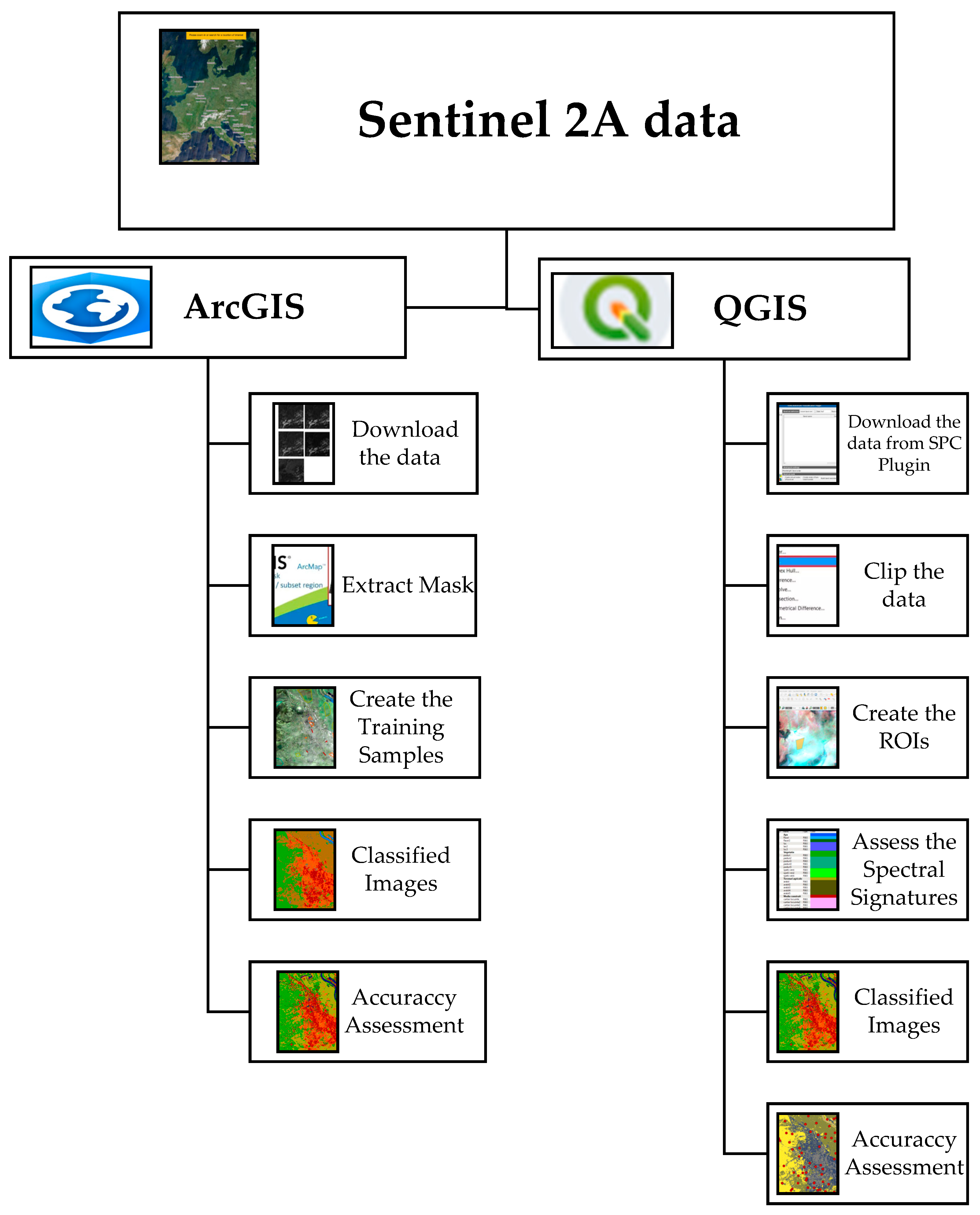
The main Land Use and Land Cover (LULC) categories in the study area include built-up areas, agricultural land (both cultivated and fallow), water bodies, and forests. The overall methodological workflow is illustrated in Figure 3. Precise identification of features such as roads, buildings, and vegetation is essential for accurate urban monitoring and natural hazard assessment. Complex and non-linear structures like urban settlements remain challenging to classify, where edge detection plays a key role in improving accuracy [39].
RGB composites (B4, B3, B2) were used for visual interpretation, enabling intuitive land cover identification. False Colour Composites were also generated to enhance vegetation detection.
The process of training sample identification and creation is a critical step, as it directly influences both the classification results and accuracy assessment [40]. The selection of appropriate samples has an even greater impact on classification accuracy than the choice of classification algorithm itself [5].

2.5. Image Pre-Processing

Image pre-processing is a crucial step that directly influences classification accuracy. It involves operations such as noise reduction, geometric correction, and radiometric normalization designed to ensure the quality and consistency of input data. The main pre-processing steps applied in this study are summarized below:
  • Clipping maps—defining and extracting the area of interest (AOI) by cutting the satellite scenes to match the study boundaries;
  • Image registration—aligning multiple image frames to ensure that corresponding elements can be accurately compared;
  • Geo-referencing—a process in which locations are assigned to images, allowing a computer to identify the location of different objects covering the terrain;
  • Radiometric correction—adjusting pixel values to normalize brightness and appearance;
  • Composite band—a composite band is generated by merging several individual spectral bands captured by remote sensing sensors. Since each band captures distinct environmental characteristics—such as surface reflectance or vegetation health—they offer complementary insights. By integrating multiple bands into a single composite image, analysts can achieve a more comprehensive representation of the landscape. These composite images are particularly valuable for identifying and mapping land use and land cover (LULC) features with greater precision;
  • Layout maps creation [41].

2.6. Satellite Image Processing
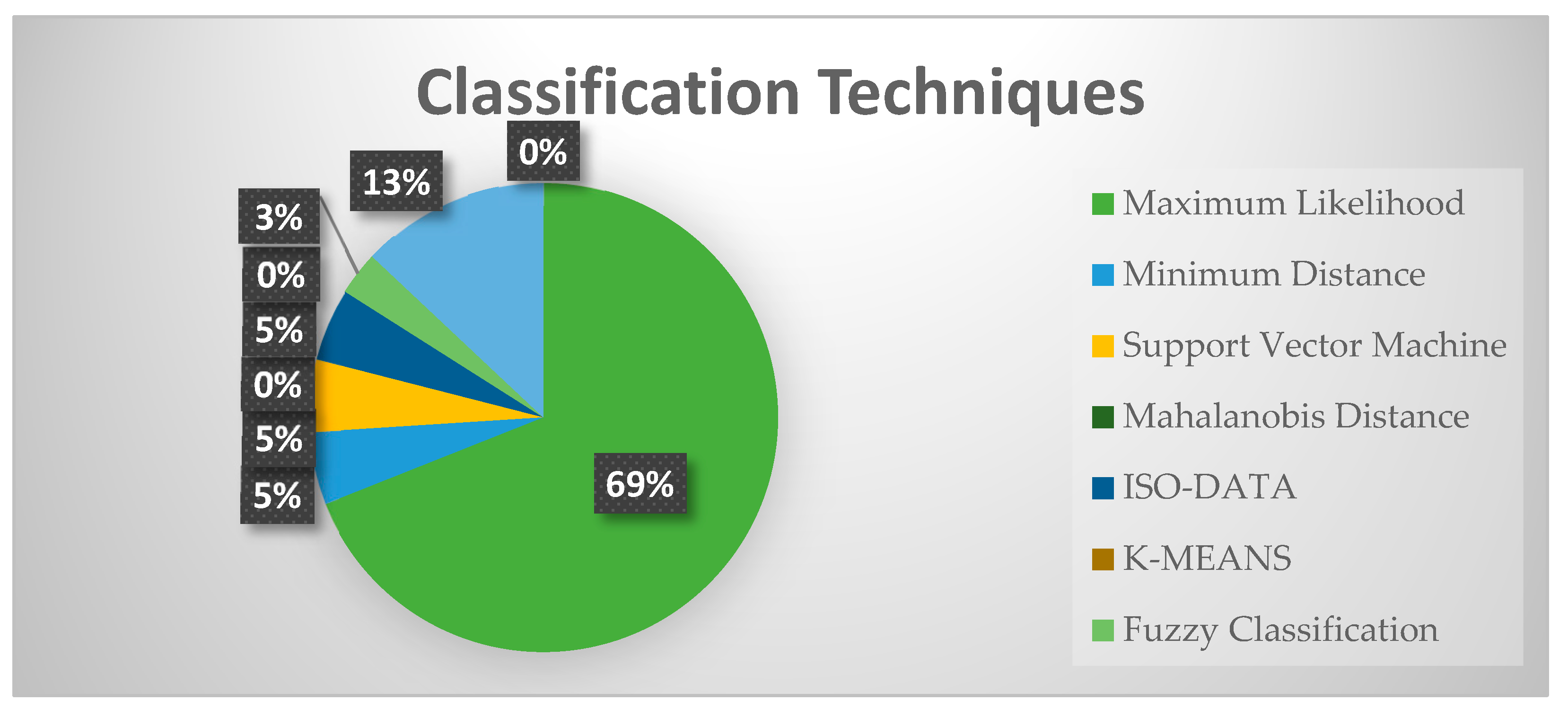
Supervised or semi-automatic classification is a technique for processing satellite imagery based on land cover categories by training an algorithm with samples containing the spectral signatures of surface features [38,42]. In essence, this method assumes prior knowledge of the study area, allowing the user to define specific land cover types and to select representative pixels corresponding to each class [43].
Figure 4 illustrates the main classification techniques. Although a wide range of satellite image classification algorithms is available, many of them exhibit limitations regarding result accuracy. These challenges often arise from the high heterogeneity within land cover classes, which makes it difficult to group pixels with diverse spectral characteristics into a single category. Furthermore, when images are affected by Gaussian or impulse noise, numerous small and fragmented regions may appear, increasing the likelihood of misclassification [44].
Figure 4. Types of the most used classification techniques, adapted from [45].
Applsci 15 11437 g004

2.7. Algorithms Used

2.7.1. Minimum Distance Algorithm

The minimum distance (MINDIST) classifier operates under the assumption that classes that are geographically or spectrally similar should be grouped together as a single prototype. This method calculates the mean spectral vector for each class and assigns pixels to the class whose prototype is closest in terms of distance [14,27]. The approach can be visualized in Figure 5a).
The MINDIST algorithm each unclassified pixel to the class with the smallest Euclidean distance in a defined space, from the unclassified pixel to the known class average [46].
The minimum distance algorithm has the disadvantage of being prone to association errors (assigning a pixel to the wrong class), because it does not take into account the variance of each class during the classification process [47].
The Semi-Automatic Classification Plugin (SCP) is a Python-based tool integrated into QGIS that facilitates image classification and is widely used in applications such as urban planning, environmental monitoring, and agriculture. The plugin allows for rapid computation by encoding contextual image information using clustering and machine learning algorithms [11]. The satellite images were imported into QGIS and atmospherically corrected prior to processing.
Subsequently, a set of Regions of Interest (ROIs) corresponding to the predefined classes, each characterized by distinct spectral signatures, was delineated to generate the training datasets. These datasets were created using the SCP interface and further processed with the scikit-learn (Python Software Foundation, Wilmington, DE, USA), which employs the Spectral Angle Mapping (SAM) algorithm to generate the final classification maps [35].

2.7.2. k-Nearest Neighbor (k-NN) Algorithm
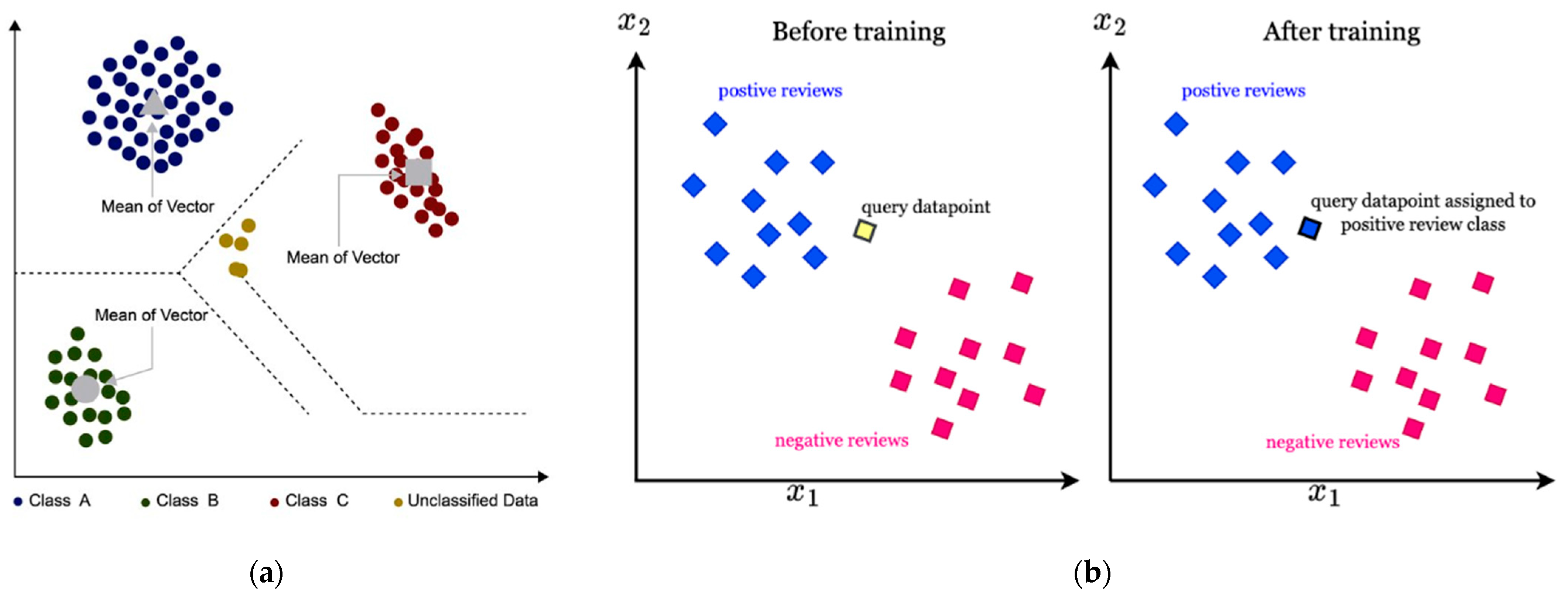
k-NN [48] is a supervised, non-parametric machine learning classification method, originally proposed in 1951. It is represented in Figure 5b). Unlike other algorithms, it does not build an explicit classification model during training; instead, it assigns a class to unknown samples based on the majority class among the k nearest training samples, determined using the Euclidean distance.
The value of the parameter k has a significant impact on the classifier’s performance: high k values can lead to over-smoothing and reduced sensitivity to local patterns, while very low k values may cause overfitting. The optimal value of k should be selected through cross-validation by testing different k values and choosing the one that provides the best classification accuracy [49].
k-NN is used for both classification and regression tasks [47]. This method is an effective option for small datasets, but in the case of large datasets, the curse of dimensionality may occur, and it is also time-consuming and resource-intensive.
Let
X = { x 1 , x 2 , , x N }
denote the training set, where each x i R n represents a data point in the n-dimensional feature space, and let
Y = { y 1 , y 2 , , y N }
represent the corresponding class labels.
In the case of a given test point x whose class is unknown, its class can be determined as follows: the similarities between the test sample and the training samples are determined using Euclidean distance, for example.
Euclidean distance (D)
D = i = 1 d ( s i x i ) 2
Identify the k nearest neighbors of the test sample within the training dataset based on similarity, and determine the class label by majority voting among these neighbors [50].
Figure 5. (a) Minimum distance classifier. Each class is represented by a mean spectral vector (centroid), and unclassified data points are assigned to the class with the shortest Euclidean distance to its centroid. This approach assumes that classes are statistically separable based on their mean vectors [51] and (b) k-NN classifies a new data point by identifying the k closest instances in the feature space and assigning the most frequent class among these neighbors [52].
Applsci 15 11437 g005

2.8. Color Samples

In ArcGIS Pro, color samples are referred to as training samples, whereas in QGIS, they are referred to as ROIs.
Selecting color samples is a crucial step, as it involves defining a group of pixels with similar spectral characteristics corresponding to each class. It is essential that the color sample contains a sufficient number of correctly labeled pixels to ensure representative training data. The resulting distributions are typically close to normal distributions, often represented as a bell-shaped curve [53].

2.9. Classification of Land Cover and Assessment of Accuracy

Color samples were manually collected [51] through visual interpretation of images provided by Sentinel-2A ((ESA, Paris, France) and Google Earth Pro (Google LLC, Mountain View, CA, USA). The classes defined in both software environments are presented in Table 2. To create the samples, polygons were uniformly distributed across the entire study area, with approximately 70 representative samples used in both case studies.
Based on the initial imagery, five classes were defined: water, buildings, vegetation, agricultural land, and infrastructure (roads and parking lots).
Accuracy assessment methods are employed to validate LULC (Land Use/Land Cover) map classifications, determining the quality of the extracted information by evaluating whether image pixels have been correctly or incorrectly classified based on remotely sensed data. These assessments can be either qualitative, involving a comparison between the classified map and real-world conditions, or quantitative, involving a detailed comparison between classified cartographic data and reference data. Accuracy assessment is essential for evaluating classification performance and supporting decision-making processes. In this study, the performance of the minimum distance and k-NN algorithms was evaluated based on the classification accuracy achieved.
The literature presents several methods for evaluating accuracy to assess the reliability of image classification, and new approaches for accuracy assessment in change detection are continually being developed. The confusion matrix, also known as the error matrix, remains the most widely used method, relying on elements such as ground control points (GCPs), the classification scheme, sample type and size, and spatial autocorrelation [45]. However, studies indicate that factors such as the methods, procedures, temporal and spatial contexts, and the choice of classification algorithm can significantly influence classification accuracy [27].
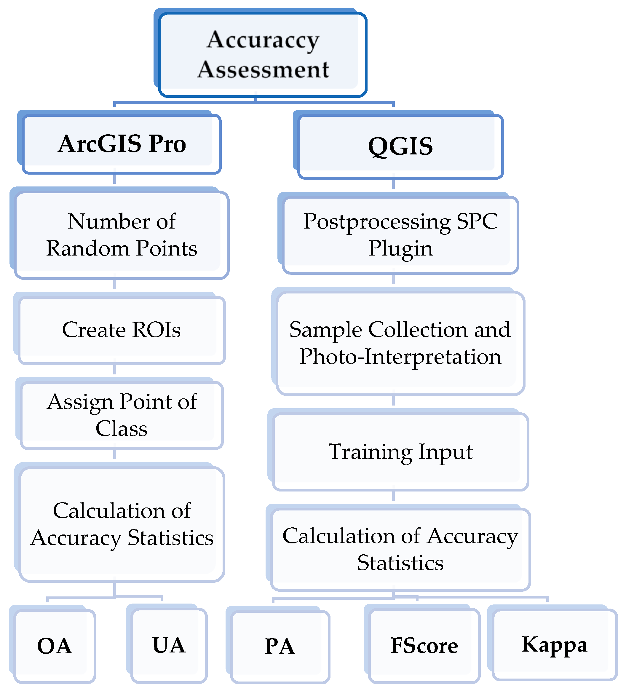
Accuracy assessment is a crucial step for interpreting results and making predictions based on them [54]. Accuracy assessment was performed following the parameters illustrated in Figure 6. The application of the workflow shown in Figure 6 results in an error matrix, where pixel values represent the comparison between the classified data and the reference data. A detailed report summarizing these values was also generated automatically by the software.
The confusion matrix is one of the most commonly used methods for evaluating classification accuracy. After post-processing, a series of parameters were calculated: Producer Accuracy (PA), User Accuracy (UA), Overall Accuracy (OA), F1 score, and the Kappa coefficient. These parameters were computed according to Equations (4)–(9).
PA and UA represent the accuracy for individual categories, while OA reflects the accuracy of the entire classification. The F1 score combines PA and UA into a single metric. The indicators were calculated as follows:
O A = i = 1 n X i i X
K a p p a = X i = 1 n X i i i = 1 n X i × X i X 2 i = 1 n X i × X i
P A = X i i X i
U A = X i i X i
F 1 s c o r e = 2 × P A × U A P A + U A
M a c r o F 1 = i = 1 n F 1 i n
where n represents the number of classes, Xii—the column, respectively, row i in the confusion matrix, representing the number of pixels in a class that are classified correctly, X is the total number of samples, Xi*—the sum of the values in row i of the confusion matrix, representing the correct number of samples of class i and X i —the sum of the values in column i, representing the number of samples assumed to be in class i [55,56].
The Kappa coefficient measures the agreement between the classified map and the ground truth [55]. We tested both classifiers—MD in QGIS and k-NN in ArcGIS Pro—and obtained different Kappa values. For Kappa coefficient values between 0.80 and 1.00, the classification can be considered highly accurate.

3. Results and Discussion

3.1. Assessment of the Accuracy of LULC Classification

In this study, three key aspects were investigated: the use of satellite imagery for land cover analysis, the comparative performance of two supervised classification algorithms, and the practical relevance of the results for enhancing urban planning and management strategies. Supervised classification was conducted in both ArcGIS Pro and QGIS environments, employing the k-Nearest Neighbor (k-NN) algorithm and the Minimum Distance (MD) classifier, respectively. To ensure methodological consistency, the same number of training samples—extracted from identical areas within Sentinel-2A imagery—was used for both classification processes.
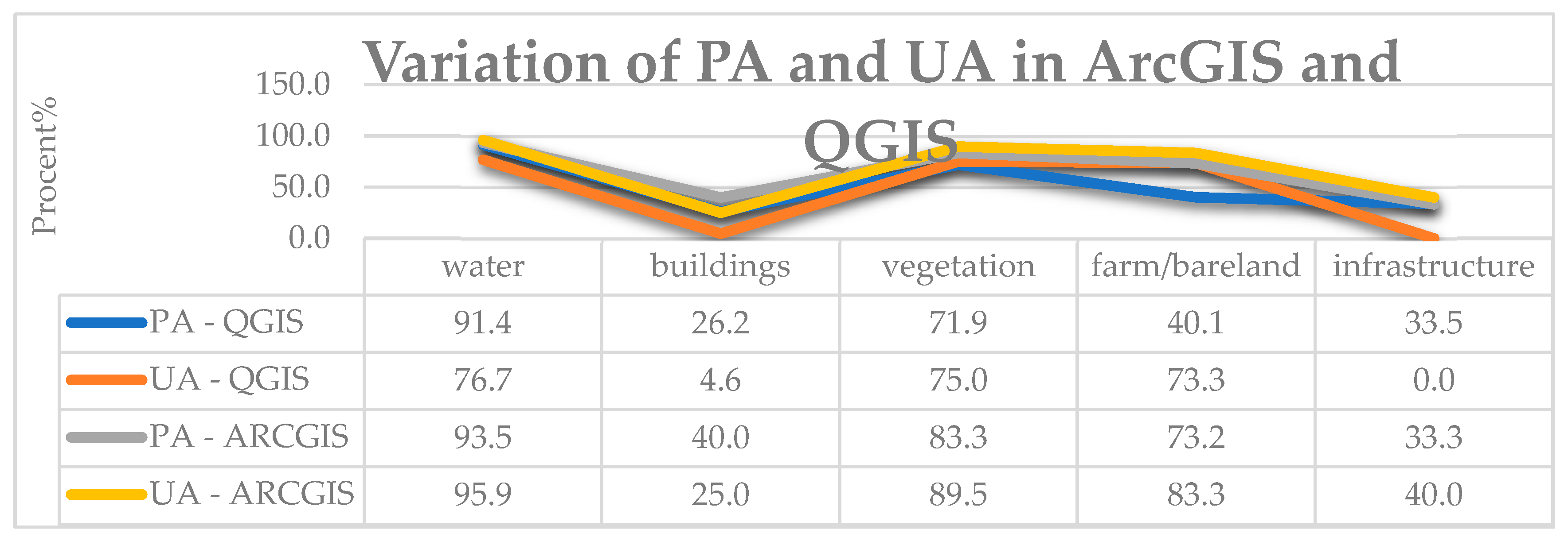
Accuracy assessment in ArcGIS Pro was performed using 100 validation points randomly distributed across the study area by the software. These points were visually interpreted and manually labeled using Google Earth Pro. The classification accuracy results are presented in Figure 7.
In QGIS, the validation was conducted using the same samples applied during classification. Visual interpretation was carried out using Google Satellite imagery, and the outcomes are summarized in Table 3. Although the Kappa coefficient indicated a satisfactory level of agreement in the QGIS classification, the k-NN algorithm in ArcGIS Pro produced superior accuracy when compared to the MD classifier. Additionally, the Overall Accuracy (OA) of the classified images was 53.53% in QGIS and 68% in ArcGIS Pro. Land Use/Land Cover (LULC) classification results following the accuracy assessment process in: (a) ArcGIS Pro using the k-NN algorithm; and (b) QGIS using the Minimum Distance classifier.

3.2. LULC Classification

For the selected study area, five land cover types were defined for the city of Deva: water, buildings, vegetation, agricultural/open land, and infrastructure.
Figure 7 illustrates that, in ArcGIS Pro, the highest similarity based on the Producer Accuracy (PA) calculation was achieved for water bodies, while the lowest PA was recorded for infrastructure.
Figure 8 illustrates the increase in reflectance within the near-infrared spectrum, primarily due to the low absorption properties of vegetation. In this urban case study, where built-up areas are predominant, artificial surfaces demonstrate generally higher reflectance across all wavelengths. In contrast, the lowest reflectance values are recorded for water bodies and infrastructure elements.
This lower accuracy is mainly due to the spectral similarity between roads, parking lots, and building rooftops, which can easily lead to classification confusion. Figure 8 also presents the spectral signature of images captured by Sentinel-2A, following classification using the SCP in QGIS and the Minimum Distance algorithm. The algorithm relies on spectral signatures, enabling the labeling of image pixels. Spectral signatures can also be used for classifying ground objects, depending on the sensor resolution and the type and extent of land cover [47].
These findings highlight the complexity of urban land cover classification due to the spectral similarity among anthropogenic surfaces. While water bodies and vegetation exhibited distinct spectral signatures that facilitated accurate classification, infrastructure elements posed challenges because of their spectral overlap with buildings and roads. Nonetheless, the comparative analysis between ArcGIS Pro and QGIS demonstrated that each platform, through its specific algorithm (k-NN and Minimum Distance, respectively), is capable of delivering valuable outputs when properly calibrated. These results support the practical applicability of open-source and proprietary GIS software in generating reliable LULC maps, especially in medium-resolution imagery contexts such as Sentinel-2A. The insights derived from this classification are essential for urban monitoring, environmental assessment, and decision-making processes related to sustainable development.

4. Discussion

The results obtained in this study indicate that the supervised classification of Sentinel-2A imagery provided a satisfactory representation of the land use and land cover (LULC) patterns in the municipality of Deva. Nevertheless, there remains potential for improvement, particularly in refining class definitions and mitigating the influence of local environmental conditions. Several factors contributed to the discrepancies observed between classification outputs. Among the most influential is the selection of land cover classes, which strongly affects the accuracy and interpretability of the final maps. For instance, the “buildings” class encompassed both apartment blocks and individual houses that differ in roofing materials, surface reflectance, and, notably, height.
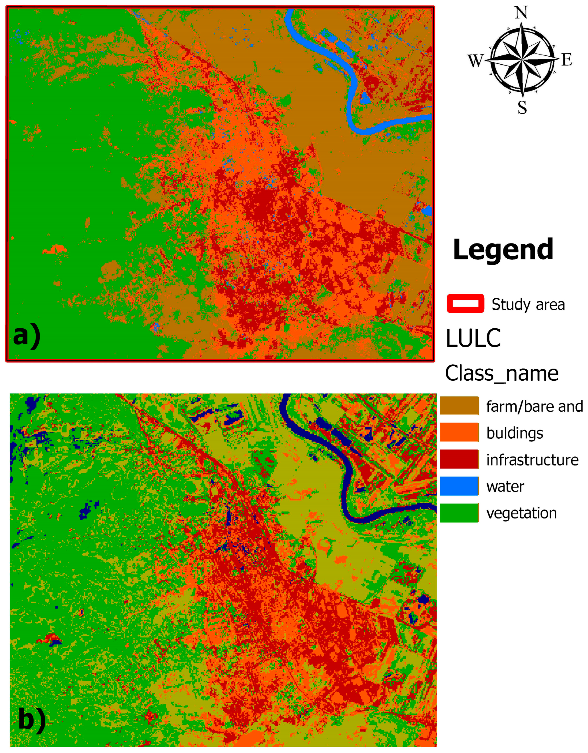
Figure 9 illustrates the results obtained through the two classifications and how we chose the training samples. Pixel-based classification methods rely exclusively on the individual spectral information of each pixel, as illustrated in Figure 8. Water bodies are characterized by low reflectance in the near-infrared (NIR) band and are generally located in low-lying and relatively flat areas (Figure 9). Consequently, the “water” class achieved the highest Producer Accuracy (PA) in both classification methods applied in this study. A similar result was also reported in the study conducted by Zhang et al. [57]. Conversely, tall buildings and roof structures generated shadows that reduced classification accuracy. The agricultural/open land category proved the most heterogeneous, encompassing a mixture of cultivated fields, grasslands, bare soil, and rocky areas. Introducing subclasses for these land types could significantly enhance classification precision. Moreover, the preprocessing of Sentinel-2A Level-2A products, which include the Scene Classification Layer (SCL), effectively mitigated common errors associated with cloud and cirrus contamination [58].
Other uncertainties, more difficult to control, may also arise, including the timing of image acquisition, seasonal variations, data consistency, spatial resolution, and the chosen processing method. In our study, it is important to note that the selected area exhibits significant elevation differences, as it is a city surrounded by mountains. In this context, shadows cast by the mountainous terrain can lead to misclassification of objects with similar spectral signatures. Therefore, we believe that the considerable variation in altitude across the mountainous and transition areas has caused vertical changes, leading to classification errors. This factor is crucial for consideration in future research [59].
Standardizing a regional classification system, supported by field-validated geospatial data, would improve the robustness and comparability of future LULC analyses. The discrepancies identified—particularly within built-up and agricultural/open land categories—highlight the potential of combining multi-source data such as Landsat, MODIS, Sentinel, or UAV imagery to enhance classification reliability. Additionally, refining the selection of training samples, both in number and representativeness, remains critical to improving overall accuracy.
Accuracy assessment in image classification aims to determine the reliability of the results by comparing the classified output with an independent reference dataset. To ensure statistical robustness, previous research emphasizes the need for a sufficient and spatially balanced number of validation samples for each land cover type. Typically, around 50 samples per class are considered adequate for a representative evaluation [60]. In our research, the sample points were manually selected, with 100 points distributed randomly in ArcGIS Pro and chosen by us in QGIS [61]. The results obtained in this study are presented in Figure 10 and Figure 11, which illustrate the land cover classification outputs generated in ArcGIS Pro and QGIS, respectively.
A previous study found that the Minimum Distance and K-Nearest Neighbors (k-NN) algorithms performed best in geomorphologically complex areas. This approach helps address the current lack of standardized methods for overcoming remote sensing limitations in mountainous regions [62].
While this approach is practical, it is susceptible to errors due to the large volume and time constraints, compounded by the quality of images from Google Earth and Google Satellite, which do not offer sufficient predictability. Furthermore, defining subclasses for the main classes could improve accuracy; for instance, in the case of the vegetation class, subclasses such as coniferous forests, beech forests, lichens, shrubs, liverworts, and similar types could be defined.
Another perspective may be to integrate SDGs with information on land classification and livelihoods in order to identify informed and sustainable decisions for urban planning [21,63].
Future research could build upon the classification maps generated in this study by comparing them with global datasets such as WorldCover or GlobCover to assess consistency across spatial scales. The possibilities for classification are vast and can be further explored by developing specific algorithms tailored to the unique characteristics of the study area in both software platforms. Comparative analyses performed on identical datasets across multiple time intervals and atmospheric conditions are recommended, as the analytical capabilities of both platforms continue to expand.

5. Conclusions

Land classification represents a fundamental component of decision-making processes in local and regional governance. When integrated with geospatial data, it provides critical insights for spatial planning and environmental management. Satellite-based remote sensing offers a cost-effective and consistent source of geospatial data over extensive areas, forming a robust foundation for land cover analysis—particularly in rapidly evolving urban environments.
Image classification was carried out using two GIS software platforms with similar performance and capabilities. Two different classifiers were employed: k-NN in ArcGIS Pro, developed by Esri [64] and the SCP in QGIS, an open-source software developed by Luca Congedo [38], using the minimum distance classifier. These classifiers were used to create maps depicting the land cover of Deva municipality and to assess the accuracy with which they were produced. Our analysis aimed to explore image processing techniques and highlight the advantages and disadvantages they generate.
In this case study, better results were obtained in terms of Overall Accuracy (OA) using ArcGIS Pro. However, the study also revealed some errors, even after post-processing, related to the terrain and topography, particularly concerning the classification of dense vegetation (forests) and arable land (cultivated land and pastures) due to the similar spectral signatures of these two classes. Similar results were found for infrastructure and buildings, as both blocks and streets share similar spectral signatures (shades of gray). The best classification results were achieved for water bodies, where the Producer Accuracy (PA) was 91.36%, User Accuracy (UA) was 76.72% in QGIS, and PA was 73.17% and UA 83.33% in ArcGIS Pro. The weakest result was obtained for infrastructure.
Several limitations should be acknowledged when interpreting these results. Classification accuracy can be influenced by model parameters, input datasets, and acquisition timing. In general, Overall Accuracy (OA) is not significantly affected by the heterogeneity of the classes, although the accuracy of User Accuracy (UA) and Producer Accuracy (PA), especially for rare classes, can be significantly influenced [48]. To minimize class bias, all seven LULC classes were assigned an equal number of training and validation samples. While an imbalanced dataset might yield higher overall accuracy by favoring dominant classes, this would compromise the reliability of individual class performance, especially for those less represented [65].
To address residual errors and improve classification accuracy, future analyses should incorporate a more detailed class hierarchy, including additional subclasses, and employ higher computational capacity to manage large datasets [48]. Another approach could involve integrating satellite images with ground control points collected for each defined class, combined with visual interpretation and classification algorithms, or higher-resolution datasets. Regarding the limitations of these methods, two aspects are particularly difficult to control: noise and clouds.
The potential of semi-automated supervised classification algorithms in the two software platforms is suitable for any geographical environment, and combining them with other types of geospatial data, such as 2D data, could increase the accuracy and reliability of the results. Therefore, maximizing the use of information obtained from remote sensing is essential, but in this study Sentinel-2 data were intentionally selected for their accessibility and cost-effectiveness compared to higher-resolution alternatives.
Future research could focus on analyzing the changes over time in the studied urban area, selecting a significant time period to study the socio-economic impact that the area has undergone. As future work, we plan to continue improving both the methods used and the exploitation of new modules, such as increasing the number of samples using augmented images, combining them with radar information, and exploring CNN architectures. Additionally, future analyses will be extended over longer time periods to better capture temporal dynamics and enhance the understanding of land use and land cover changes.

Author Contributions

Conceptualization, O.M.B. and A.C.B.; methodology, O.M.B.; investigation, O.M.B.; resources, O.M.B., G.B. and A.C.B.; data curation, O.M.B.; writing—original draft preparation, O.M.B.; writing—review and editing, O.M.B., A.C.B., P.I.D., G.B.; visualization, O.M.B., G.B., A.C.B. and P.I.D.; supervision, G.B., A.C.B. and P.I.D. All authors have read and agreed to the published version of the manuscript.

Funding

This research received no external funding.

Data Availability Statement

Data available on request due to privacy restrictions.

Acknowledgments

This study was conducted within the Geodetic Engineering Measurements and Spatial Data Infrastructures Research Centre, Faculty of Geodesy, Technical University of Civil Engineering Bucharest. This study was conducted using Esri software (version 2.9.2) licenses provided by the Doctoral School of the Technical University of Civil Engineering Bucharest. QGIS (version 7.10.11) is an opensource software.

Conflicts of Interest

The authors declare no conflicts of interest.

References

  1. Oli, D.; Gyawali, B.; Neupane, B.; Oshikoya, S. Assessment of Land Use Land Cover Change and Its Impact on Variations of Land Surface Temperature in Atlanta, USA. Environ. Sustain. Indic. 2025, 26, 100712. [Google Scholar] [CrossRef]
  2. Ursu, C.-D.; Benedek, J.; Temerdek-Ivan, K. Accuracy Assessment of Four Land Cover Datasets at Urban, Rural and Metropolitan Area Level. Remote Sens. 2025, 17, 756. [Google Scholar] [CrossRef]
  3. Said, Y.; Saidani, O.; Algarni, A.D.; Algarni, M.H.; Flah, A. Lightweight Multiscale Information Aggregation Network for Land Cover Land Use Semantic Segmentation from Remote Sensing Images. Sci. Rep. 2025, 15, 30265. [Google Scholar] [CrossRef]
  4. Frimpong, B.F.; Molkenthin, F. Tracking Urban Expansion Using Random Forests for the Classification of Landsat Imagery (1986–2015) and Predicting Urban/Built-Up Areas for 2025: A Study of the Kumasi Metropolis, Ghana. Land 2021, 10, 44. [Google Scholar] [CrossRef]
  5. Simoes, R.; Camara, G.; Queiroz, G.; Souza, F.; Andrade, P.R.; Santos, L.; Carvalho, A.; Ferreira, K. Satellite Image Time Series Analysis for Big Earth Observation Data. Remote Sens. 2021, 13, 2428. [Google Scholar] [CrossRef]
  6. Chachondhia, P.; Shakya, A.; Kumar, G. Performance Evaluation of Machine Learning Algorithms Using Optical and Microwave Data for LULC Classification. Remote Sens. Appl. Soc. Environ. 2021, 23, 100599. [Google Scholar] [CrossRef]
  7. Hysa, A.; Spalevic, V.; Dudic, B.; Roșca, S.; Kuriqi, A.; Bilașco, Ș.; Sestras, P. Utilizing the Available Open-Source Remotely Sensed Data in Assessing the Wildfire Ignition and Spread Capacities of Vegetated Surfaces in Romania. Remote Sens. 2021, 13, 2737. [Google Scholar] [CrossRef]
  8. Landsat Satellite Missions|U.S. Geological Survey. Available online: https://www.usgs.gov/landsat-missions/landsat-satellite-missions (accessed on 26 May 2025).
  9. Copernicus S2 Mission. Available online: https://sentiwiki.copernicus.eu/web/s2-mission (accessed on 26 May 2025).
  10. Phiri, D.; Simwanda, M.; Salekin, S.; Nyirenda, V.; Murayama, Y.; Ranagalage, M. Sentinel-2 Data for Land Cover/Use Mapping: A Review. Remote Sens. 2020, 12, 2291. [Google Scholar] [CrossRef]
  11. Tempa, K.; Aryal, K.R. Semi-Automatic Classification for Rapid Delineation of the Geohazard-Prone Areas Using Sentinel-2 Satellite Imagery. SN Appl. Sci. 2022, 4, 141. [Google Scholar] [CrossRef]
  12. Yuan, Y.; Lin, L.; Liu, Q.; Hang, R.; Zhou, Z.-G. SITS-Former: A Pre-Trained Spatio-Spectral-Temporal Representation Model for Sentinel-2 Time Series Classification. Int. J. Appl. Earth Obs. Geoinf. 2022, 106, 102651. [Google Scholar] [CrossRef]
  13. Nasiri, V.; Deljouei, A.; Moradi, F.; Sadeghi, S.M.M.; Borz, S.A. Land Use and Land Cover Mapping Using Sentinel-2, Landsat-8 Satellite Images, and Google Earth Engine: A Comparison of Two Composition Methods. Remote Sens. 2022, 14, 1977. [Google Scholar] [CrossRef]
  14. Nivedita Priyadarshini, K.; Kumar, M.; Rahaman, S.A.; Nitheshnirmal, S. A Comparative Study of Advanced Land Use/Land Cover Classification Algorithms Using Sentinel-2 Data. Int. Arch. Photogramm. Remote Sens. Spat. Inf. Sci. 2018, XLII–5, 665–670. [Google Scholar] [CrossRef]
  15. Copernicus. Available online: https://www.copernicus.eu/en (accessed on 26 May 2025).
  16. Sudmanns, M.; Tiede, D.; Augustin, H.; Lang, S. Assessing Global Sentinel-2 Coverage Dynamics and Data Availability for Operational Earth Observation (EO) Applications Using the EO-Compass. Int. J. Digit. Earth 2020, 13, 768–784. [Google Scholar] [CrossRef]
  17. Cai, B.; Shao, Z.; Huang, X.; Zhou, X.; Fang, S. Deep Learning-Based Building Height Mapping Using Sentinel-1 and Sentinel-2 Data. Int. J. Appl. Earth Obs. Geoinf. 2023, 122, 103399. [Google Scholar] [CrossRef]
  18. Habibie, M.I.; Nurda, N.; Fernando, D.; Arifandri, R.; Putra, P.K.; Prayogi, H.; Sencaki, D.B. Integrating Sentinel-2 and ESA World Cover for Effective Land Use and Land Cover Assessment Using Machine Learning. Adv. Space Res. 2025, 76, 4925–4958. [Google Scholar] [CrossRef]
  19. Yimer, S.M.; Bouanani, A.; Kumar, N.; Tischbein, B.; Borgemeister, C. Comparison of Different Machine-Learning Algorithms for Land Use Land Cover Mapping in a Heterogenous Landscape over the Eastern Nile River Basin, Ethiopia. Adv. Space Res. 2024, 74, 2180–2199. [Google Scholar] [CrossRef]
  20. Ismail, M.A.; Muhamad Ludin, A.N.; Hosni, N. Comparative Assessment of the Unsupervised Land Use Classification by Using Proprietary GIS and Open Source Software. IOP Conf. Ser. Earth Environ. Sci. 2020, 540, 012020. [Google Scholar] [CrossRef]
  21. Cloete, D.N.; Shoko, C.; Dube, T.; Clarke, S. Remote Sensing-Based Land Use Land Cover Classification for the Heuningnes Catchment, Cape Agulhas, South Africa. Phys. Chem. Earth Parts A/B/C 2024, 134, 103559. [Google Scholar] [CrossRef]
  22. Yuh, Y.G.; Tracz, W.; Matthews, H.D.; Turner, S.E. Application of Machine Learning Approaches for Land Cover Monitoring in Northern Cameroon. Ecol. Inform. 2023, 74, 101955. [Google Scholar] [CrossRef]
  23. Cuypers, S.; Nascetti, A.; Vergauwen, M. Land Use and Land Cover Mapping with VHR and Multi-Temporal Sentinel-2 Imagery. Remote Sens. 2023, 15, 2501. [Google Scholar] [CrossRef]
  24. Zaki, A.; Buchori, I.; Sejati, A.W.; Liu, Y. An Object-Based Image Analysis in QGIS for Image Classification and Assessment of Coastal Spatial Planning. Egypt. J. Remote Sens. Space Sci. 2022, 25, 349–359. [Google Scholar] [CrossRef]
  25. Suh, C.N.; Tsheko, R.; Kayombo, B.; Moroke, S.T. Analysis of Land Cover Land Use Change in the Greater Gaborone Area of South Eastern Botswana. Acta Ecol. Sin. 2023, 43, 1080–1089. [Google Scholar] [CrossRef]
  26. Stoica, I.-V.; Vîrghileanu, M.; Zamfir, D.; Mihai, B.-A.; Săvulescu, I. Comparative Assessment of the Built-Up Area Expansion Based on Corine Land Cover and Landsat Datasets: A Case Study of a Post-Socialist City. Remote Sens. 2020, 12, 2137. [Google Scholar] [CrossRef]
  27. Basheer, S.; Wang, X.; Farooque, A.A.; Nawaz, R.A.; Liu, K.; Adekanmbi, T.; Liu, S. Comparison of Land Use Land Cover Classifiers Using Different Satellite Imagery and Machine Learning Techniques. Remote Sens. 2022, 14, 4978. [Google Scholar] [CrossRef]
  28. Afuye, G.A.; Nduku, L.; Kalumba, A.M.; Santos, C.A.G.; Orimoloye, I.R.; Ojeh, V.N.; Thamaga, K.H.; Sibandze, P. Global Trend Assessment of Land Use and Land Cover Changes: A Systematic Approach to Future Research Development and Planning. J. King Saud. Univ.- Sci. 2024, 36, 103262. [Google Scholar] [CrossRef]
  29. Geospatial Information and the 2030 Agenda for Sustainable Development. Available online: https://www.unescap.org/resources/stats-brief-december-2020-issue-no-27-geospatial-information-and-2030-agenda-sustainable (accessed on 26 May 2025).
  30. Cardenas-Ritzert, O.S.E.; Vogeler, J.C.; Shah Heydari, S.; Fekety, P.A.; Laituri, M.; McHale, M.R. Effects of Land Use Data Spatial Resolution on SDG Indicator 11.3.1 (Urban Expansion) Assessments: A Case Study Across Ethiopia. Sustainability 2024, 16, 9698. [Google Scholar] [CrossRef]
  31. Praticò, S.; Solano, F.; Di Fazio, S.; Modica, G. Machine Learning Classification of Mediterranean Forest Habitats in Google Earth Engine Based on Seasonal Sentinel-2 Time-Series and Input Image Composition Optimisation. Remote Sens. 2021, 13, 586. [Google Scholar] [CrossRef]
  32. Wikipedia. Deva, Romania. Available online: https://en.wikipedia.org/wiki/Deva,_Romania (accessed on 17 October 2025).
  33. National Agency for Natural Protected Areas (ANANP). Protected Natural Areas of Romania. Available online: https://ananp.gov.ro/ariile-naturale-protejate-ale-romaniei/ (accessed on 16 October 2025).
  34. Romanian National Meteorological Administration (ANM). Available online: https://www.meteoromania.ro (accessed on 17 October 2025).
  35. Sawant, S.; Garg, R.D.; Meshram, V.; Mistry, S. Sen-2 LULC: Land Use Land Cover Dataset for Deep Learning Approaches. Data Brief. 2023, 51, 109724. [Google Scholar] [CrossRef]
  36. Huang, H.; Roy, D.; Boschetti, L.; Zhang, H.; Yan, L.; Kumar, S.; Gomez-Dans, J.; Li, J. Separability Analysis of Sentinel-2A Multi-Spectral Instrument (MSI) Data for Burned Area Discrimination. Remote Sens. 2016, 8, 873. [Google Scholar] [CrossRef]
  37. Sentinel-2A SatelliteSensor|Satellite Imaging Corp. Available online: https://www.satimagingcorp.com/satellite-sensors/other-satellite-sensors/sentinel-2a/ (accessed on 17 October 2025).
  38. Semi-Automatic Classification Plugin—QGIS Python Plugins Repository. Available online: https://plugins.qgis.org/plugins/SemiAutomaticClassificationPlugin/ (accessed on 26 May 2025).
  39. Asokan, A.; Anitha, J.; Ciobanu, M.; Gabor, A.; Naaji, A.; Hemanth, D.J. Image Processing Techniques for Analysis of Satellite Images for Historical Maps Classification—An Overview. Appl. Sci. 2020, 10, 4207. [Google Scholar] [CrossRef]
  40. Zhang, H.; He, J.; Chen, S.; Zhan, Y.; Bai, Y.; Qin, Y. Comparing Three Methods of Selecting Training Samples in Supervised Classification of Multispectral Remote Sensing Images. Sensors 2023, 23, 8530. [Google Scholar] [CrossRef]
  41. Darem, A.A.; Alhashmi, A.A.; Almadani, A.M.; Alanazi, A.K.; Sutantra, G.A. Development of a Map for Land Use and Land Cover Classification of the Northern Border Region Using Remote Sensing and GIS. Egypt. J. Remote Sens. Space Sci. 2023, 26, 341–350. [Google Scholar] [CrossRef]
  42. Gondwe, J.F.; Lin, S.; Munthali, R.M. Analysis of Land Use and Land Cover Changes in Urban Areas Using Remote Sensing: Case of Blantyre City. Discret. Dyn. Nat. Soc. 2021, 2021, 8011565. [Google Scholar] [CrossRef]
  43. Ramjeawon, M.; Demlie, M.; Toucher, M.L.; Van Rensburg, S.J. Analysis of Three Decades of Land Cover Changes in the Maputaland Coastal Plain, South Africa. KOEDOE Afr. Prot. Area Conserv. Sci. 2020, 62, a1642. [Google Scholar] [CrossRef]
  44. Espinola, M.; Piedra-Fernandez, J.A.; Ayala, R.; Iribarne, L.; Wang, J.Z. Contextual and Hierarchical Classification of Satellite Images Based on Cellular Automata. IEEE Trans. Geosci. Remote Sens. 2015, 53, 795–809. [Google Scholar] [CrossRef]
  45. Chughtai, A.H.; Abbasi, H.; Karas, I.R. A Review on Change Detection Method and Accuracy Assessment for Land Use Land Cover. Remote Sens. Appl. Soc. Environ. 2021, 22, 100482. [Google Scholar] [CrossRef]
  46. Stern, A.J.; Daughtry, C.S.T.; Hunt, E.R.; Gao, F. Comparison of Five Spectral Indices and Six Imagery Classification Techniques for Assessment of Crop Residue Cover Using Four Years of Landsat Imagery. Remote Sens. 2023, 15, 4596. [Google Scholar] [CrossRef]
  47. Trigunasih, N.M.; Narka, I.W.; Saifulloh, M. Mapping Eruption Affected Area Using Sentinel-2A Imagery and Machine Learning Techniques. J. Degrade. Min. Land. Manag. 2023, 11, 5073. [Google Scholar] [CrossRef]
  48. Maxwell, A.E.; Warner, T.A.; Fang, F. Implementation of Machine-Learning Classification in Remote Sensing: An Applied Review. Int. J. Remote Sens. 2018, 39, 2784–2817. [Google Scholar] [CrossRef]
  49. Ge, G.; Shi, Z.; Zhu, Y.; Yang, X.; Hao, Y. Land Use/Cover Classification in an Arid Desert-Oasis Mosaic Landscape of China Using Remote Sensed Imagery: Performance Assessment of Four Machine Learning Algorithms. Glob. Ecol. Conserv. 2020, 22, e00971. [Google Scholar] [CrossRef]
  50. Boateng, E.Y.; Otoo, J.; Abaye, D.A. Basic Tenets of Classification Algorithms K-Nearest-Neighbor, Support Vector Machine, Random Forest and Neural Network: A Review. JDAIP 2020, 8, 341–357. [Google Scholar] [CrossRef]
  51. Razaque, A.; Ben Haj Frej, M.; Almi’ani, M.; Alotaibi, M.; Alotaibi, B. Improved Support Vector Machine Enabled Radial Basis Function and Linear Variants for Remote Sensing Image Classification. Sensors 2021, 21, 4431. [Google Scholar] [CrossRef] [PubMed]
  52. K-Nearest Neighbors (KNN) Algorithm for Classification: Real-world Applications and Examples. Available online: https://www.linkedin.com/pulse/k-nearest-neighbors-knn-algorithm-classification-nrxgf (accessed on 16 July 2025).
  53. Understanding Segmentation and Classification—ArcGIS Pro|Documentation. Available online: https://pro.arcgis.com/en/pro-app/latest/help/analysis/image-analyst/understanding-segmentation-and-classification.htm# (accessed on 9 April 2024).
  54. Sensing, R.; Change, L.C.; Areas, U.; Detection, C. Remote Sensing-Based Urban Land Use/Land Cover Change Detection and Monitoring. J. Remote Sens. GIS 2017, 6, 3. [Google Scholar] [CrossRef]
  55. Feng, F.; Gao, M.; Liu, R.; Yao, S.; Yang, G. A Deep Learning Framework for Crop Mapping with Reconstructed Sentinel-2 Time Series Images. Comput. Electron. Agric. 2023, 213, 108227. [Google Scholar] [CrossRef]
  56. Billah, M.; Islam, A.K.M.S.; Mamoon, W.B.; Rahman, M.R. Random Forest Classifications for Landuse Mapping to Assess Rapid Flood Damage Using Sentinel-1 and Sentinel-2 Data. Remote Sens. Appl. Soc. Environ. 2023, 30, 100947. [Google Scholar] [CrossRef]
  57. Zhang, X.; Du, L.; Tan, S.; Wu, F.; Zhu, L.; Zeng, Y.; Wu, B. Land Use and Land Cover Mapping Using RapidEye Imagery Based on a Novel Band Attention Deep Learning Method in the Three Gorges Reservoir Area. Remote Sens. 2021, 13, 1225. [Google Scholar] [CrossRef]
  58. Kang, J.; Yang, X.; Wang, Z.; Cheng, H.; Wang, J.; Tang, H.; Li, Y.; Bian, Z.; Bai, Z. Comparison of Three Ten Meter Land Cover Products in a Drought Region: A Case Study in Northwestern China. Land 2022, 11, 427. [Google Scholar] [CrossRef]
  59. Zhang, B.; Liu, L.; Zhang, Y.; Wei, B.; Gong, D.; Li, L. Spatial Consistency and Accuracy Analysis of Multi-Source Land Cover Products on the Southeastern Tibetan Plateau, China. Remote Sens. 2024, 16, 3219. [Google Scholar] [CrossRef]
  60. Kasahun, M.; Legesse, A. Machine Learning for Urban Land Use/Cover Mapping: Comparison of Artificial Neural Network, Random Forest and Support Vector Machine, a Case Study of Dilla Town. Heliyon 2024, 10, e39146. [Google Scholar] [CrossRef]
  61. Alshari, E.A.; Gawali, B.W. Development of Classification System for LULC Using Remote Sensing and GIS. Glob. Transit. Proc. 2021, 2, 8–17. [Google Scholar] [CrossRef]
  62. Orusa, T.; Cammareri, D.; Borgogno Mondino, E. A Possible Land Cover EAGLE Approach to Overcome Remote Sensing Limitations in the Alps Based on Sentinel-1 and Sentinel-2: The Case of Aosta Valley (NW Italy). Remote Sens. 2022, 15, 178. [Google Scholar] [CrossRef]
  63. Tasnim, S.; Mahbub, F.; Biswas, G.; Enamul Haque, D.M. Spatial Indices and SDG Indicator-Based Urban Environmental Change Detection of the Major Cities in Bangladesh. J. Urban. Manag. 2022, 11, 519–529. [Google Scholar] [CrossRef]
  64. Esri Desktop GIS Software|Mapping Analytics|ArcGIS Pro. Available online: https://www.esri.com/en-us/arcgis/products/arcgis-pro/overview (accessed on 26 May 2023).
  65. McCarty, D.A.; Kim, H.W.; Lee, H.K. Evaluation of Light Gradient Boosted Machine Learning Technique in Large Scale Land Use and Land Cover Classification. Environments 2020, 7, 84. [Google Scholar] [CrossRef]
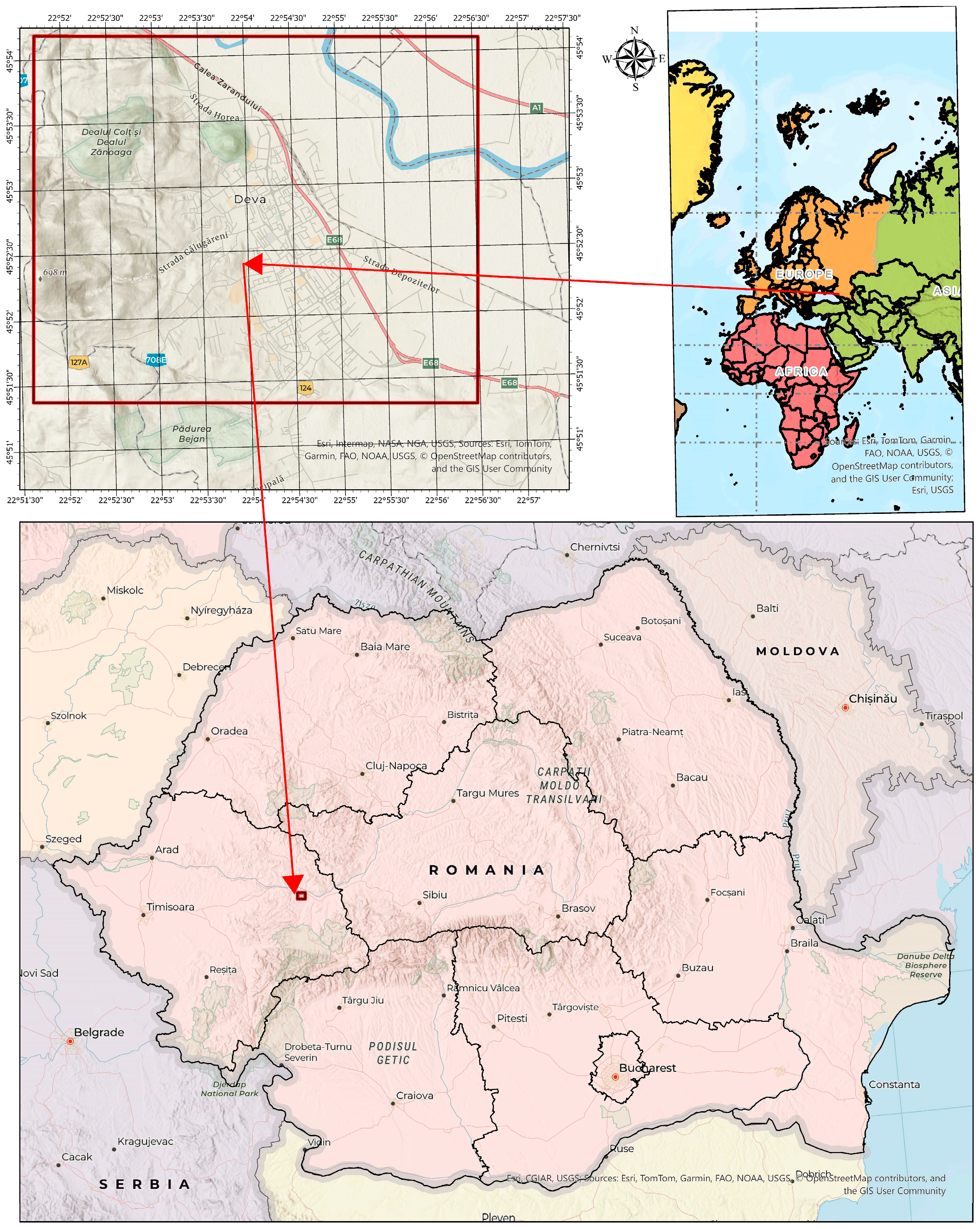
Figure 1. Map of the study area—Deva municipality (source: authors).
Applsci 15 11437 g001
Figure 2. Sentinel-2 spectral bands used in the classification process. The figure illustrates ten gray scale images corresponding to spectral bands B2 (Blue), B3 (Green), B4 (Red), B5, B6, B7, B8 (Near-Infrared), B8A, B11 (Short-Wave Infrared 1), and B12 (Short-Wave Infrared 2). These bands were selected due to their relevance in distinguishing between various land cover types such as built-up areas, vegetation, and water bodies. Each image highlights specific reflectance characteristics that contribute to the spectral separability of surface features. (source: ESA, Paris, France).
Applsci 15 11437 g002
Figure 3. Workflow carried out using the software ArcGIS Pro and QGIS. Both ArcGIS Pro and QGIS support preparatory workflows for supervised classification. In ArcGIS Pro, training samples are digitized per class, while in QGIS, Spatial Point Clustering (SPC) applied to ROIs enables automatic identification of homogeneous training regions. (source: authors).
Applsci 15 11437 g003
Figure 6. Workflow for accuracy assessment applied in ArcGIS Pro and QGIS. OA—Overall Accuracy; UA—User’s Accuracy; PA—Producer’s Accuracy; FScore—F1-score; Kappa—Cohen’s Kappa coefficient. The workflow shows the specific steps followed by the authors in each software environment to calculate classification accuracy metrics. (source: authors).
Applsci 15 11437 g006
Figure 7. UA = user accuracy și PA = producer accuracy. They were obtained in both software programs. Comparison between the two analyses.
Applsci 15 11437 g007
Figure 8. Signature reflectance in different land cover types. Spectral reflectance profiles of different land cover classes across multiple wavelength ranges. Vegetation exhibits a distinct increase in reflectance in the near-infrared region (~7.5 µm), while water bodies show consistently low reflectance values. Built-up surfaces (infrastructure and buildings) display moderate, relatively uniform reflectance across all bands. These spectral differences support land cover classification based on supervised algorithms.
Applsci 15 11437 g008
Figure 9. Land Use/Land Cover (LULC) classification results following the accuracy assessment process in: (a) ArcGIS Pro using the k-NN algorithm; and (b) QGIS using the Minimum Distance classifier.
Applsci 15 11437 g009
Figure 10. Classification map of the study area created in ArcGIS Pro: (a’) Google Earth image high lighting the river and the corresponding classified area (a), (b’) Urban area view from Google Earth and the classification result of the same classified area (b), (c’) Forested area view from Google Earth and the classification result (c) of the same area.
Applsci 15 11437 g010
Figure 11. Classification map of the study area created in QGIS: (a’) Google Earth image highlighting the river and the corresponding classified area (a), (b’) Urban area view from Google Satellite and the classification result of the same classified area (b), (c’) Forested area view from Google Satellite and the classification result (c) of the same area.
Applsci 15 11437 g011
Table 2. Description of land classification in this study.
No.ClassesDescription
1WaterRivers, lakes, pools, ponds
2BuildingResidential, commercial, industrial, transportation
3VegetationForests, parks, green spaces
4Agricultural LandArable land with less than 10% vegetation cover
5InfrastructureStreets, bridges, parking lots, platforms
Table 3. Interpretation of the Kappa coefficient, adapted from [25].
CoefficientIntervalAccuracyQGIS (SPC)ArcGIS Pro
0.4–0.6good0.320.54
Kappa0.6–0.8very good--
0.8–1.00excellent--
Disclaimer/Publisher’s Note: The statements, opinions and data contained in all publications are solely those of the individual author(s) and contributor(s) and not of MDPI and/or the editor(s). MDPI and/or the editor(s) disclaim responsibility for any injury to people or property resulting from any ideas, methods, instructions or products referred to in the content.