Article

Target Tracking with Adaptive Morphological Correlation and Neural Predictive Modeling

by
Victor H. Diaz-Ramirez
1,* and
Leopoldo N. Gaxiola-Sanchez
2
1
Instituto Politécnico Nacional—CITEDI, Ave. Instituto Politécnico Nacional 1310, Tijuana 22435, BC, Mexico
2
Tecnológico Nacional de México, Instituto Tecnológico de Culiacán, Juan de Dios Bátiz 310, Culiacán 80220, SIN, Mexico
*
Author to whom correspondence should be addressed.
Appl. Sci. 2025, 15(21), 11406; https://doi.org/10.3390/app152111406
Submission received: 27 September 2025 / Revised: 17 October 2025 / Accepted: 22 October 2025 / Published: 24 October 2025
(This article belongs to the Special Issue Application of Artificial Intelligence in Image Processing)

Abstract

A tracking method based on adaptive morphological correlation and neural predictive models is presented. The morphological correlation filters are optimized according to the aggregated binary dissimilarity-to-matching ratio criterion and are adapted online to appearance variations of the target across frames. Morphological correlation filtering enables reliable detection and accurate localization of the target in the scene. Furthermore, trained neural models predict the target’s expected location in subsequent frames and estimate its bounding box from the correlation response. Effective stages for drift correction and tracker reinitialization are also proposed. Performance evaluation results for the proposed tracking method on four image datasets are presented and discussed using objective measures of detection rate (DR), location accuracy in terms of normalized location error (NLE), and region-of-support estimation in terms of intersection over union (IoU). The results indicate a maximum average performance of 90.1% in DR, 0.754 in IoU, and 0.004 in NLE on a single dataset, and 83.9%, 0.694, and 0.015, respectively, across all four datasets. In addition, the results obtained with the proposed tracking method are compared with those of five widely used correlation filter-based trackers. The results show that the suggested morphological-correlation filtering, combined with trained neural models, generalizes well across diverse tracking conditions.

1. Introduction

Visual object tracking is a central problem in computer vision owing to its broad utility across high-impact applications, including video surveillance, autonomous navigation, human–computer interaction, biomedical imaging, and robotics.
Object tracking consists of estimating the time-varying state (e.g., position and region of support) of a target across an image sequence as it moves through the field of view. This problem is challenging because captured image sequences are often degraded by sensor noise, nonuniform illumination, and blur degradation, among others. Additionally, the target can exhibit appearance changes (pose, rotation, scale), and captured scene images can contain background clutter, partial or prolonged occlusions, and out-of-view events. Furthermore, for applications with real-time constraints, high-rate tracking is important. Because of these factors, tracker designs must achieve both robustness and computational efficiency [1].
Over the years, numerous methods have been proposed to address real-world tracking problems [2,3,4]. Several methods employ offline training, in which a model is pre-trained on labeled data that include the target (true class) and unwanted patterns from the background and distractor objects (false class) before tracking begins [5,6]. Other methods utilize an online training approach that is initialized from minimal target information in the initial frame and adapts the model during tracking operation [7,8]. Online adaptation offers greater flexibility under appearance changes of the target and scene over time. Online training is often preferred in single-object tracking, in which the target exhibits unseen appearance variations during tracking. Also, there are hybrid tracking methods that combine robust offline-learned representations with online learning to balance accuracy and adaptability [9,10].
A successful online training approach to target tracking is tracking-by-detection. This approach learns a discriminative classifier online to distinguish the target from the background. For each frame, image fragments at multiple scales are extracted around the predicted target location. Next, the candidate bounding box with the highest score is selected as the target’s estimate, and the model is updated with new true-class templates near the predicted target location and false-class templates taken from the background. This approach adapts well to appearance variations and is robust to clutter. However, it is sensitive to sensor noise and weakly regularized online updates, which can lead to overfitting and drift.
A widely used tracker within this approach is Multiple Instance Learning (MIL) [11]. MIL considers the training data collected during tracking as bags of candidate image fragments. Positive bags contain at least one true target instance, while negative bags contain only background fragments. Updating the classifier with weak set-level supervision mitigates label uncertainty and enables adaptation to gradual appearance drift.
The Structured Output Tracking with Kernels (Struck) [12] is a widely used tracker that learns a structured support vector machine that directly scores candidate bounding boxes, relating the target’s location space to the online training samples. Struck has demonstrated strong performance on several standard datasets [4].
Another successful tracker is Tracking–Learning–Detection (TLD) [13], which integrates a short-term tracker with a long-term detector and an online learning component. Using a boosted classifier with consistency constraints and a sampling strategy, TLD yields robustness to occlusions and appearance variations. Despite strong performance, the tracking-by-detection approach is computationally intensive because it requires evaluating large sets of candidate templates and updating the classifier every frame, increasing latency.
An alternative widely used approach for target tracking consists of correlation filtering. In this approach, a linear filter is trained to produce a sharp correlation peak at the target location. Next, target detection and filter adaptation are performed efficiently in the Fourier domain by exploiting the convolution theorem [14,15]. A successful approach for correlation filter design consists of employing ridge regularization. In this formulation, the filter is constructed by solving a least-squares problem with 2 regularization, aimed at controlling overfitting and improving numerical stability. Spatial and temporal regularizers constrain the target’s region of support and promote smooth evolution across frames, improving robustness to clutter and appearance changes.
The Kernelized Correlation Filters (KCFs) [16] are designed by solving a kernelized ridge regression problem on dense circular shifts of the target template using prespecified Gaussian-shaped desired correlation responses. This approach yields good performance under small translations and moderate appearance changes of the target. Additionally, it is suitable for real-time operation. However, the circular boundary assumption induces boundary artifacts and wrap-around effects that introduce background content into the true-class samples, potentially increasing drift errors. In addition, the absence of scale adaptation and of long-term re-detection stages makes this method prone to target loss.
Spatially Regularized Discriminative Correlation Filters (SRDCFs) [17,18] are constructed by solving a kernelized ridge regression problem with spatially varying regularization that penalizes coefficients increasingly with distance from the target origin. This spatial weighting confines the region of support for the target, mitigates boundary artifacts, and enables training with a larger search area while reducing background influence. Compared with KCF, SRDCF improves localization accuracy and robustness in cluttered scenes. A main drawback of SRDCF is the increased computational cost due to spatial regularization and its sensitivity to the spatial weight design. A successful variant of SRDCF incorporates adaptive decontamination of the training set to suppress corrupted samples caused by occlusions, background clutter, or misalignment [19]. This variant is referred to as SRDCFd. During online learning, contaminated updates are identified and assigned reduced weights, which improves peak localization and detection performance in cluttered scenes. A potential drawback is the increased computational cost and limited adaptation when few uncontaminated samples are available.
Background-Aware Correlation Filters (BACFs) [20,21], are learned by solving a ridge regression problem on circulant samples extracted from an enlarged search region. A cropping operator enforces zero coefficients outside the target template, thereby limiting the region of support to the object region. This background-aware formulation provides the learning process from false patterns, alleviating boundary artifacts and improving discrimination in cluttered scenes. Compared with KCF, SRDCF, and SRDCFd, BACF provides improved robustness to scene degradations and false objects. An important limitation of BACF is its higher optimization cost and increased sensitivity to the crop ratio and to the regularization parameters.
Spatial–Temporal Regularized Correlation Filters (STRCFs) [22], are designed using ridge regression with both spatial and temporal regularization. The spatial term penalizes coefficients with increasing distance from the target center, confining the region of support of the filter to the target’s region and mitigating boundary artifacts while reducing background influence. The temporal term penalizes deviations of the filter from the previous frame, stabilizing updates and reducing drift under appearance changes. Compared with KCF, SRDCF, SRDCFd, and BACF, STRCF improves robustness to deformations of the target and partial occlusions. However, this method has two main limitations. First, the spatial and temporal terms increase computational cost. Second, the temporal-regularization term introduces temporal inertia, delaying adaptation under abrupt changes.
In contrast, this work presents an alternative approach for designing correlation filters for target tracking using a morphological-based formulation. The proposed filters are optimized with respect to the Aggregated Binary Dissimilarity-to-Matching Ratio (ABDR) criterion. Because morphological correlation is applied to images after binary threshold decomposition, the resulting filters are more robust to illumination variations and sensor noise. In addition, we introduce a correlation-plane postprocessing method based on synthetic-basis projection that suppresses clutter-induced correlation responses, improving the reliability of target detection. Furthermore, we incorporate trained neural models to predict the target’s center location and estimate the bounding box of the detected target. The proposed tracking method also includes efficient stages for drift correction and tracking reinitialization, improving robustness. As a result, the proposed tracking approach enables accurate estimation of the target state (location and bounding box) in image sequences under challenging conditions such as abrupt motion, partial occlusions, nonrigid deformations, and nonuniform illumination. The main contributions of this research are summarized as follows:
  • Morphological-correlation filter design: An adaptive correlation filtering method based on morphological operations is proposed for robust target tracking, providing an alternative to the conventional ridge-regularization formulation and improving robustness to scene perturbations.
  • Correlation-plane postprocessing: A postprocessing stage based on synthetic-basis projection is introduced to refine the correlation response and improve target detection in cluttered scenes.
  • Hybrid tracking framework: A tracking approach is developed that integrates an online-trained morphological correlation for target detection with neural models trained offline for target location prediction and bounding box estimation, achieving stable tracking trajectories across frames.
  • Drift-correction and reinitialization mechanisms: Efficient methods for drift correction and tracking reinitialization are incorporated to maintain tracking stability under occlusions, illumination variations, and temporary target loss.
This paper is organized as follows. Section 2 describes the proposed method for target tracking based on morphological correlation and neural predictive models. First, we present the design of morphological correlation filters. Next, we detail the suggested postprocessing stage for correlation plane denoising. We then describe the operation steps of the proposed tracking method. Section 3 presents the results of the proposed tracking method using four widely used image datasets. Tracking performance is quantified using objective measures of detection efficiency, target location accuracy, and bounding box estimation. We also compare the performance of the proposed tracking method with that of five widely used correlation filter-based trackers. Finally, Section 4 presents the conclusions.

2. Proposed Target Tracking Method

Here, we describe the proposed approach for single-object tracking based on morphological correlation filtering and neural predictive models. Section 2.1 details reliable target detection using morphological correlation filtering. Section 2.2 introduces postprocessing of the correlation plane using synthetic basis projection. Section 2.3 presents the complete tracking algorithm.

2.1. Target Recognition Based on Morphological Correlation

Let t ( x , y ) be a reference view of a target object to be recognized, located at the arbitrary coordinates ( x t , y t ) in a captured image of a scene, f ( x , y ) , given as
f ( x , y ) = t ( x x t , y y t ) + m ( x x t , y y t ) b ( x , y ) + n ( x , y ) ,
where n ( x , y ) is additive sensor noise, b ( x , y ) is the image of the background, and m ( x , y ) is the inverse support function of the target, given by
m ( x , y ) = 0 , if ( x , y ) t ( x , y ) 1 , otherwise .
In conventional correlation pattern recognition [23], the coordinates of the target in the scene are estimated using the linear correlation, as follows:
( x ^ t , y ^ t ) = arg max ( x , y ) R 2 f ( τ x , τ y ) h ( x + τ x , y + τ y ) d τ x d τ y ,
where h ( x , y ) is the impulse response of a correlation filter. In recent decades, numerous filter designs have been proposed to optimize different performance criteria [24]. Interested readers are invited to consult the following references: [25,26,27,28,29]. A key advantage of using Equation (3) for target recognition is its efficient frequency-domain computation with the Fast Fourier Transform (FFT) [14,30]. However, a main limitation of this approach for target tracking is that, to construct and update the filter for each captured frame, explicit knowledge of the target’s region of support m ( x , y ) , as well as a statistical characterization of b ( x , y ) and n ( x , y ) , is required. Consequently, it is necessary to incorporate reliable algorithms to estimate these components dynamically, thereby potentially reducing both recognition performance and computational efficiency.
The proposed approach based on morphological correlation achieves high recognition performance without requiring explicit knowledge of the target’s region of support in each frame, nor estimation of the statistical characteristics of the background and sensor noise.
Consider a digital image I ( x , y ) with the size of N x × N y elements. This image can be represented through a binary threshold decomposition as follows [31,32]:
I ( x , y ) = ( v min 1 ) + v = v min v max I v ( x , y ) ,
where ( v min , v max ) denote the minimum and maximum intensity values of I ( x , y ) , with v min 1 and v max v min , and
I v ( x , y ) = 1 , if I ( x , y ) v , 0 , otherwise ,
is the binary image corresponding to I ( x , y ) at the threshold level v. In Equations (4) and (5),
I ˜ ( x , y ) = v = v min v max I v ( x , y )
is a preprocessed version of I ( x , y ) , obtained by applying a binary threshold decomposition (BTD). Note that if v min = 1 , then I ˜ ( x , y ) = I ( x , y ) .
In this scenario, to reliably detect and locate the target t ( x , y ) in the input image f ( x , y ) , the Aggregated Binary Dissimilarity-to-Matching Ratio (ABDR) is defined as follows:
ABDR ( τ x , τ y ) = v = v min v max x , y t v ( x , y ) f v ( x τ x , y τ y ) v = v min v max x , y t v ( x , y ) + f v ( x τ x , y τ y ) 1 ,
where t v ( x , y ) and f v ( x , y ) are binary images of t ( x , y ) and f ( x , y ) , respectively, as given in Equation (5). The numerator in Equation (7) is the aggregated binary dissimilarity between t ( x , y ) and f ( x , y ) at the coordinates ( τ x , τ y ) , whereas the denominator is the aggregated binary matching score. The ABDR is zero when the two compared images are identical and tends to infinity when there are no matching elements between them.
Considering the identity min I 1 , v ( x , y ) + I 2 , v ( x , y ) , 1 = max I 1 , v ( x , y ) , I 2 , v ( x , y ) [33], Equation (7) can be rewritten as follows:
ABDR ( τ x , τ y ) = μ t + μ f 2 V N v v = v min v max x , y min t v ( x , y ) , f v ( x τ x , y τ y ) 1 + μ t + μ f 2 V N v v = v min v max x , y max t v ( x , y ) , f v ( x τ x , y τ y ) ,
where μ t and μ f are the local mean intensity values of t ( x , y ) and f ( x , y ) , respectively, V = ( v max v min ) is the number of threshold values in the decomposition, and N v = N x × N y is the total number of image elements.
The minimum value of Equation (8) is reached when maximizing the correlation
C ( τ x , τ y ) = v = v min v max x , y min t v ( x , y ) , f v ( x τ x , y τ y ) 1 V N v + v = v min v max x , y max t v ( x , y ) , f v ( x τ x , y τ y ) ,
where the term ( 1 / V N v ) is added to the denominator to avoid division by zero.
The computational efficiency of Equation (9) can be improved by interchanging the order of the summation and applying the generalized morphological identity [31]:
v = v min v max I 1 , v ( x , y ) , I 2 , v ( x , y ) = I ˜ 1 ( x , y ) , I ˜ 2 ( x , y ) ,
where { min , max } . As a result, the morphological correlation in Equation (9) can be expressed as follows:
C ( τ x , τ y ) = x , y min t ˜ ( x , y ) , f ˜ ( x τ x , y τ y ) 1 V N v + x , y max t ˜ ( x , y ) , f ˜ ( x τ x , y τ y ) .
The coordinates of the target in the scene are estimated from Equation (10) as follows:
( τ ˜ x , τ ˜ y ) = arg max τ x , τ y C ( τ x , τ y ) .
In Equation (10), t ˜ ( x , y ) and f ˜ ( x , y ) denote the preprocessed versions of the reference image t ( x , y ) and input image f ( x , y ) obtained through binary threshold-decomposition.
The robustness of target recognition using morphological correlation can be improved by selecting the values { v min , v max } that characterize the object located at the origin of the image I i ( x , y ) , where I i ( x , y ) corresponds to either t ( x , y ) or f ( x , y ) . These limits can be defined as follows:
v min = I i ( 0 , 0 ) ϵ v σ I i , v max = I i ( 0 , 0 ) + ϵ v σ I i ,
where σ I i denotes the standard deviation of I i ( x , y ) relative to the value at the origin I i ( 0 , 0 ) , and ϵ v is a dispersion coefficient. Additionally, by specifying the number of quantization levels Q and defining the quantization step
Δ v = 2 ϵ v σ v Q ,
the resulting binary threshold decomposed images are given by
t ˜ ( x , y ) = v = 1 Q t ( v min + v Δ v ) ( x , y ) , f ˜ ( x τ x , y τ y ) = v = 1 Q f ( v min + v Δ v ) ( x τ x , y τ y ) .
The preprocessed images given in Equation (14) are employed in Equation (10) to reliably detect the target in a captured scene image.

2.2. Postprocessing of the Correlation Plane Through Synthetic Basis Projection

The robustness of target detection using morphological correlation filtering can be improved via projection-based postprocessing. This approach involves the construction of two sets of synthetic bases a priori: one composed of noise-free correlation planes that model the expected responses produced by the target, and another set composed of realizations of spatially correlated noise to model the responses of the background or false objects. The observed correlation plane is reconstructed as a combination of the synthetic basis functions and a residual term. The postprocessed (denoised) plane is obtained by isolating the component associated with the synthetic correlation planes and removing the contribution from the noise realizations. This simple procedure minimizes false-detection errors and improves the reliability of target detection.
The set of N p noise-free synthetic correlation planes { C k ( x , y ) : k = 1 , , N p } is generated using an inverse-polynomial model of the form
C k ( x , y ) = 1 + ( x x k ) 2 + ( y y k ) 2 b k 2 α ,
where ( x k , y k ) specify the coordinates of the correlation peak, b k is a scale parameter controlling the spatial spread, and α is a fixed shape parameter that defines the decay rate. Each synthetic plane produces a single peak located near the origin, with variations in peak width introduced through different values of b k . Furthermore, the set of N p synthetic noise patterns { η k ( x , y ) : k = 1 , , N p } is generated by applying a smoothing filter to two-dimensional white noise realizations, inducing spatial correlation.
The amplitude values of each synthetic correlation plane C k ( x , y ) are lexicographically reordered into column vectors c k . Then, a matrix of vectorized correlation planes is constructed as follows:
Y C = [ c 1 , c 2 , , c N p ] .
To ensure that Y C is full rank, its columns can be orthogonalized using Singular Value Decomposition (SVD). Similarly, each noise pattern η k ( x , y ) is reordered into a column vector η k , which is used to construct the following matrix:
Y η = [ η 1 , η 2 , , η N p ] .
In this manner, the regressor matrix is constructed as follows:
A = Y C Y η .
From Equation (18), the observed correlation plane can be reconstructed as follows:
c = A β + r ,
where β is a vector of weighting coefficients, and r is the residual term. The weighting coefficients can be obtained by solving the regularized least squares problem:
β = arg min β A β c 2 + λ β 2 ,
where λ > 0 is a regularization parameter. Note that the objective function A β c 2 is convex and differentiable. Thus, taking its gradient with respect to β and setting it to zero yields the following:
( A A + λ I ) β = A c .
The linear system in Equation (21) can be solved efficiently using Cholesky decomposition, since the matrix A A + λ I is symmetric and positive definite.
Note that the correlation plane reconstructed using only the synthetic planes is c r = A β . Thus, the residual term can be computed as r = c c r , and the denoised correlation plane is obtained as follows:
c ^ = Y C β C + r ,
where β C is the vector containing the first N p elements of β . Finally, the resultant vector c ^ is reshaped into a two-dimensional array C ^ ( x , y ) .
Next, a subpixel-accurate Fourier shift can be applied to C ^ ( x , y ) for correcting the displacement of the correlation peak introduced during postprocessing. The shifted plane is computed as follows:
C ^ sh ( x , y ) = F 1 F C ^ ( x , y ) · e j 2 π Δ x · u N x + Δ y · v N y ,
where ( Δ x , Δ y ) represent the coordinate displacement between the peak location ( τ ^ x , τ ^ y ) of the observed correlation plane and that of the postprocessed plane, and “ F { · } , F 1 { · } ” denote the two-dimensional Fourier and inverse Fourier transforms, respectively.

2.3. Target Tracking Based on Morphological Correlation Filtering and Neural Predictive Models

The proposed tracking algorithm consists of a sequence of processing stages, as shown in Figure 1. The algorithm begins by capturing an image frame of the scene, from which the target object is selected either manually or automatically to create a target template. The central coordinates of this template are considered to be the current coordinates ( x t , y t ) of the target. This template is then preprocessed using BTD, as defined in Equation (14).
Afterwards, a new image frame is captured, and a region of interest (ROI) is extracted with origin on the coordinates ( x t , y t ) . The morphological correlation given in Equation (10) is then computed and postprocessed using Equations (22) and (23) between the preprocessed target template and the ROI to perform target detection. The detection stage determines if the target is successfully recognized within the ROI.
If detection is successful, the target bounding box is predicted using the designed CNN-based model described in Appendix A.2. The coordinates of the target in the current frame are then estimated from the ROI, as given in Equation (11). The target template t i ( x , y ) is also updated using the estimated coordinates of the current target detection. To improve robustness, a drift estimation and correction step is incorporated. This stage estimates a small translational offset, which is used to align the target’s template before updating it. The proposed drift correction method is detailed in Appendix B. The target’s template for detecting the target in the next frame is dynamically adapted as follows:
t i ( x , y ) = ( 1 β ) t i ( x , y ) + β t i 1 ( x , y ) ,
where t i 1 ( x , y ) is the past target template and β is a forgetting parameter (usually β = 0.125 ). The coordinates of the target for the next frame are then predicted using the designed NN-based model described in Appendix A.1, which uses the past five estimated target locations.
Details of the trained neural models are provided in Appendix A.1 and Appendix A.2. The target position prediction model was trained using a dataset consisting of five-element coordinate vectors derived from annotated image sequences. The bounding box estimation model was trained using a dataset composed of image fragments of 321 × 321 pixels containing targets of varying sizes and background complexity. The data were normalized and randomly partitioned into training and validation subsets with a 70–30 ratio to promote generalization capability. To reduce the risk of overfitting, particularly in cases involving small targets or cluttered scenes, the models incorporated batch normalization and dropout layers, and a mild form of data augmentation was applied during training.
If the target is not detected, the algorithm performs a reinitialization stage, which is detailed in Appendix C, to re-detect the target across the entire scene image. This procedure employs a sliding window approach that evaluates each window location within the scene based on a similarity metric combining Histogram of Oriented Gradients (HOG) and color histogram features. The region of the scene that has the highest similarity score with respect to the archived target’s features is selected as the new bounding box, allowing the tracker to resume operation. This reinitialization step improves robustness against occlusions, appearance changes, and unexpected tracking failures.
The proposed algorithm shown in Figure 1 enables reliable target detection, accurate localization, precise bounding box estimation, and online adaptation throughout the image sequence, yielding efficient and robust tracking.

3. Results

This section presents the results of the proposed tracking method based on morphological correlation and neural predictive modeling. Tracking performance is evaluated using objective measures on video sequences from four widely used datasets. Furthermore, the performance of the proposed method is compared with that of five widely used correlation-based tracking methods.
Section 3.1 describes the experiments performed, including the input image sequences used for tracking evaluation, the performance measures considered to assess the effectiveness of the proposed and existing tracking methods, and the implementation details. Section 3.3 presents the performance results of the proposed and existing methods. Section 3.4 analyzes and discusses the results.

3.1. Description of Experiments

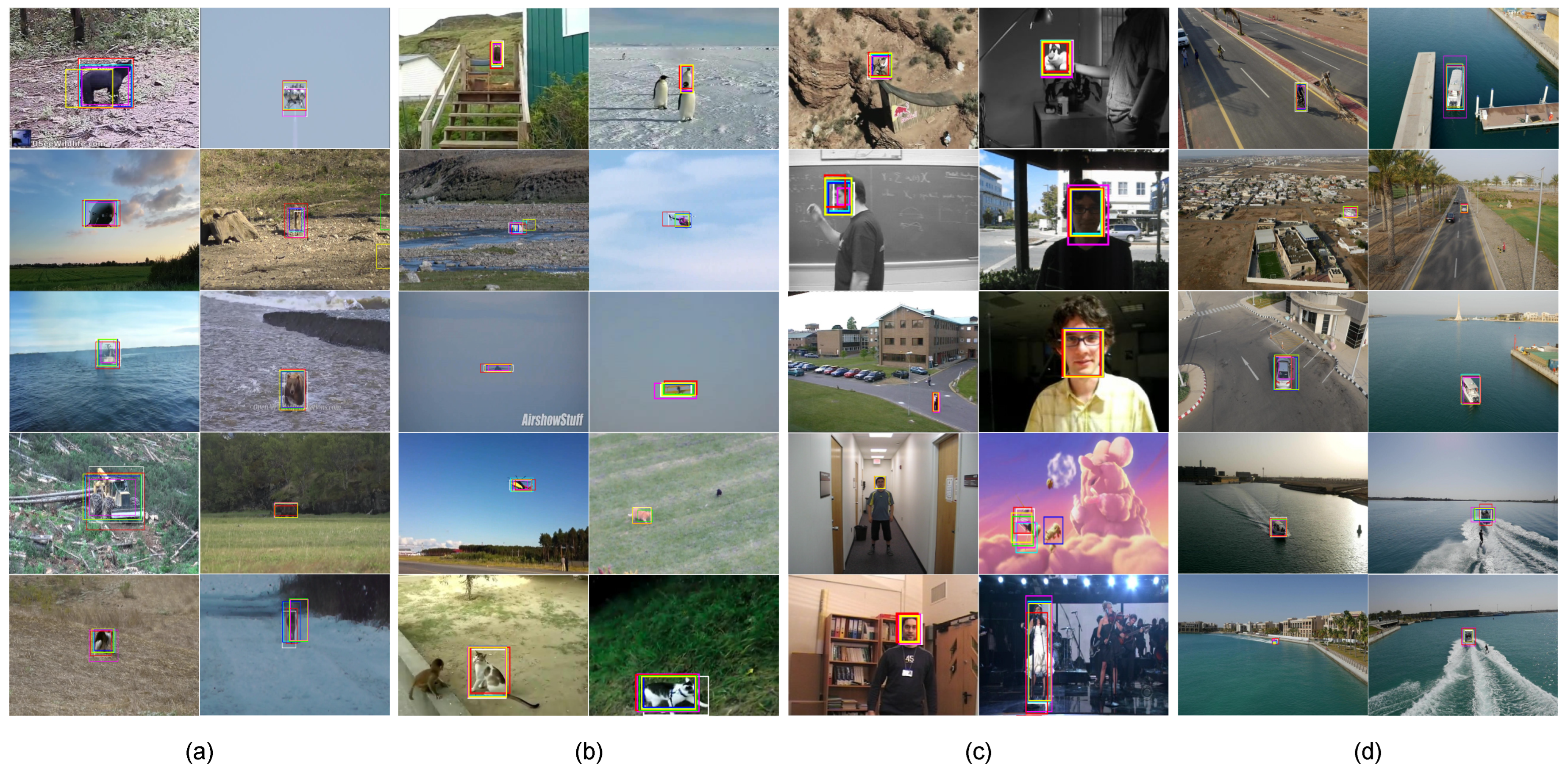
To evaluate the performance of the proposed tracking method, we considered input test sequences from four different widely used and distinct datasets: Large-scale Single Object Tracking (LaSOT) [34], Generic Object Tracking Benchmark (GOT-10k) [35], A Benchmark and Simulator for UAV Tracking (UAV123) [36], and Object Tracking Benchmark (OTB50) [4]. These datasets cover a wide range of target tracking challenges, including deformations and variations in scale, nonuniform illumination, background clutter, occlusions, and abrupt camera motion. Consequently, these datasets enable a comprehensive evaluation of tracker robustness under diverse visual conditions. We employed ten video sequences from each dataset, yielding a total of 38,484 frames distributed as follows: 1195 frames from GOT-10k, 22,853 frames from LaSOT, 4527 frames from OTB50, and 9991 frames from UAV123. Figure 2 shows representative test frames extracted from the selected sequences within each of the four evaluated datasets. Each frame in Figure 2 shows the target estimated by the proposed method, referred to as Morphological Correlation Filtering (MCF), highlighted with a red bounding box. For performance comparison, we evaluated five correlation-based trackers: Kernelized Correlation Filters (KCFs) [16] (magenta), Spatial–Temporal Regularized Correlation Filters (STRCFs) [22] (blue), Background-Aware Correlation Filters (BACFs) [21] (cyan), SRDCF [17] (green), and SRDCF with adaptive template decontamination (SRDCFd) [19] (yellow). Note that the estimate produced by the MCF method closely matches the ground truth, which is highlighted with a white bounding box.

Performance Evaluation Metrics

Tracking performance is evaluated using three criteria: accuracy of the target’s center location, accuracy of the target’s bounding box overlap, and detection rate. Typically, the accuracy and robustness of the target’s center-location estimation and bounding box overlap are characterized by two commonly used metrics: precision and success.
The precision metric assesses the accuracy of the predicted target’s center location by computing the Euclidean distance between the centers of the predicted bounding box and the corresponding ground truth. Let ( x t i , y t i ) and ( x g i , y g i ) denote the centers of the predicted and ground truth bounding boxes at frame i, respectively. The normalized location error (NLE) is given by
NLE i = 1 D ( x t i x g i ) 2 + ( y t i y g i ) 2 ,
where D = W 2 + H 2 is the frame diagonal length, with W and H denoting the frame width and height, respectively. The precision score is given by the proportion of frames where NLE i is below a specified threshold τ , as follows:
Precision = 1 N i = 1 N I NLE i < τ ,
where N is the total number of frames and
I ( A ) = 1 if A is true , 0 if A is false .
The success metric evaluates the overlap between the predicted bounding box B t i and the ground-truth bounding box B g i at each frame. Consider the Intersection over Union (IoU) metric, which quantifies the spatial overlap between the estimated box B t i and the ground-truth box B g i and is computed as follows:
IoU i = | B t i B g i | | B t i B g i | ,
where | · | denotes the area of a region. The success metric consists of the fraction of frames in which IoU i exceeds a threshold τ [ 0 , 1 ] , defined as follows:
Success = 1 N i = 1 N I IoU i > τ .
Another important characteristic of a tracking algorithm is the detection rate (DR), defined as the percentage of frames for which the tracker detects the target and successfully estimates its state. In this work, the target is considered detected if IoU i τ , with τ = 0.5 . Thus, the DR can be computed as follows:
DR = 100 N i = 1 N I IoU i 0.5 .

3.2. Implementation Details

The proposed method was implemented in Python 3.13.2 using NumPy 2.2.6, Numba 0.61.2, OpenCV 4.11.0, SciPy 1.15.2, scikit-image 0.25.2, and PyTorch 2.7.0. The existing methods, KCF [16], STRCF [22], BACF [20], SRDCF [17], and SRDCFd [19], were run in MATLAB R2024b using the authors’ released code. The experiments were carried out on a MacBook Pro computer equipped with an Apple M3 Max processor and 64 GB of RAM, running macOS 15.5.

3.3. Performance Evaluation Results

The tracking performance of the proposed method and the considered correlation-based methods is evaluated by processing 40 videos from the GOT-10k, LaSOT, OTB50, and UAV123 datasets, as shown in Figure 2. For all trackers, the initial target location and bounding box are initialized from the ground-truth annotation of the datasets. For each subsequent frame in the sequence, the tracker estimates the target state (center coordinates and bounding box). Additionally, the NLE and IoU metrics are computed between the tracker’s estimate and the ground-truth annotation. Table 1 presents, for each tracker, the mean ± standard deviation of NLE and IoU, computed over all sequences shown in Figure 2 across the four datasets, as well as the percentage of DR. We observe that the proposed MCF tracker achieves the best overall performance and the best results on most datasets. On the GOT-10k dataset, the MCF and BACF trackers achieve the lowest NLE among all evaluated trackers. However, MCF outperforms BACF in terms of IoU and DR. The STRCF tracker performs slightly below BACF, whereas the SRDCF, SRDCFd, and KCF trackers achieve lower performance on this dataset.
On the LaSOT dataset, the MCF tracker produces the best results among all tested trackers in terms of NLE, IoU, and DR. The STRCF tracker achieves performance comparable to that of MCF in terms of NLE. However, the MCF tracker outperforms STRCF in terms of DR and IoU. The BACF tracker exhibits performance comparable to that of STRCF, achieving a higher DR. The SRDCF and SRDCFd trackers exhibit moderate performance, whereas KCF achieves the lowest performance among the evaluated trackers. Note that the LaSOT dataset presents more difficult tracking challenges, including very long sequences that can induce drift errors, out-of-view events, and long occlusions that make consistent target detection difficult, as well as large appearance changes of the target and strong perturbations, such as non-uniform illumination and background clutter.
On the OTB50 dataset, the MCF tracker yields the lowest NLE, indicating the best center-location accuracy. The STRCF tracker achieves slightly higher IoU and DR than the MCF tracker. The BACF tracker performs comparably to the MCF tracker. The SRDCF and SRDCFd trackers produce competitive results, and the KCF tracker exhibits the weakest performance among the evaluated methods.
On the UAV123 dataset, the proposed MCF tracker achieves the best results among all evaluated methods in terms of NLE, IoU, and DR. The BACF tracker produces competitive results in terms of IoU and DR. The SRDCF and SRDCFd trackers also exhibit good performance, whereas the KCF tracker produces the worst results. Across all datasets combined, the proposed MCF tracker achieves the best overall performance in terms of NLE, IoU, and DR values, indicating that the morphological correlation filtering combined with the trained neural predictive models generalizes well across diverse tracking conditions, particularly on larger and more challenging datasets (GOT-10k, LaSOT, UAV123).
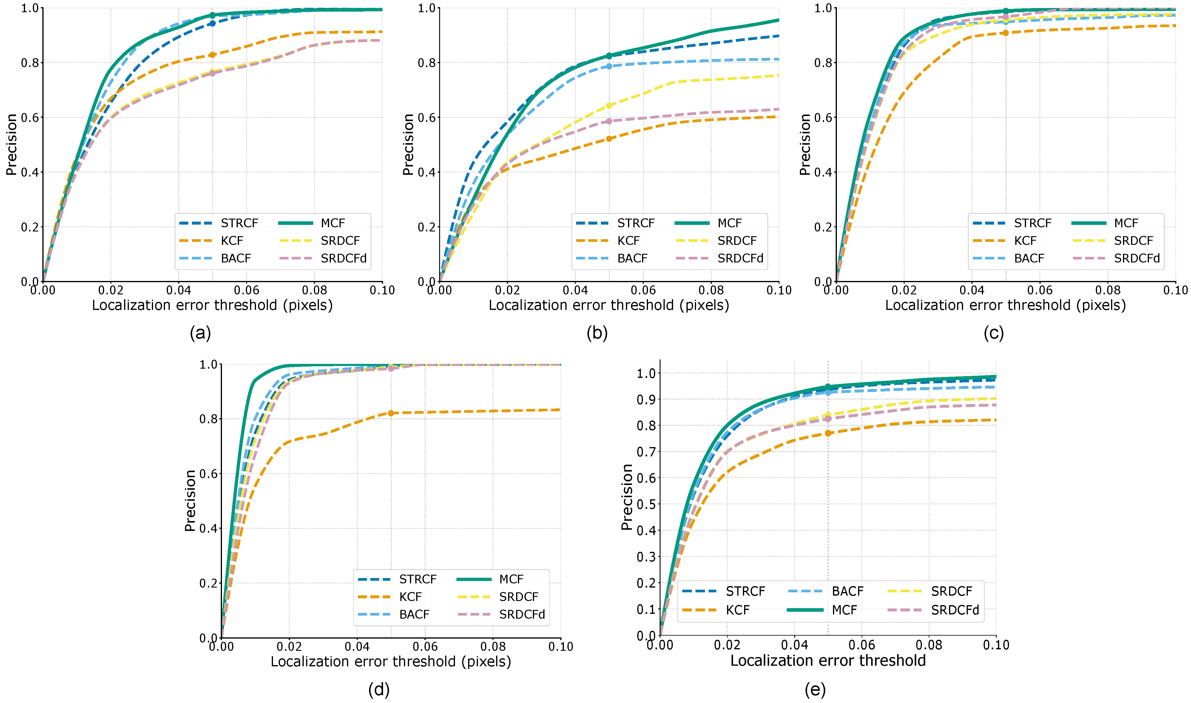
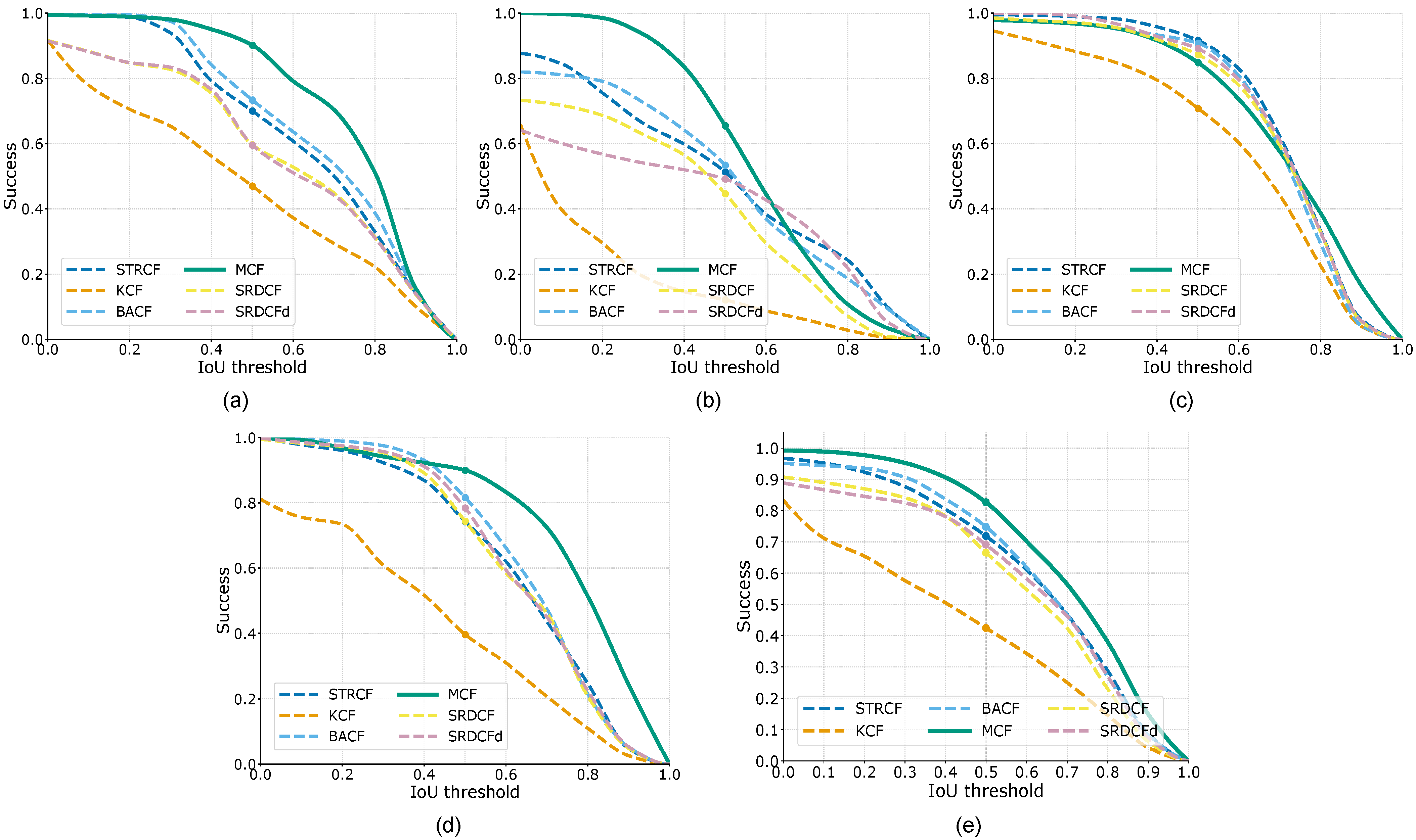
Furthermore, to evaluate robustness, we computed precision and success plots for the proposed MCF tracker and the considered trackers across all datasets. These plots are shown in Figure 3 and Figure 4. Precision plots depict, as a function of the NLE threshold, the fraction of frames for which the center-location error falls below the threshold, whereas success plots depict, as a function of the IoU threshold, the fraction of frames for which the overlap exceeds the threshold. These results plots characterize a tracker’s localization accuracy and robustness across operating points. The area under the curve (AUC) serves as a single scalar metric, obtained by integrating the curve over the threshold range.
On the GOT-10k dataset, the MCF tracker with precision AUC of 0.846 and success AUC of 0.748 yields the best results. The BACF and STRCF trackers are competitive, yielding precision AUCs of 0.840 and 0.817 and success AUCs of 0.675 and 0.649, respectively. The KCF, SRDCF, and SRDCFd trackers yield the worst results. On the LaSOT dataset, the MCF and STRCF trackers achieve the highest center-location accuracy, each with a precision AUC of 0.724. In terms of IoU-based success, MCF achieves the best performance, with a success AUC of 0.575. The BACF tracker yields competitive performance, with a precision AUC of 0.670 and a success AUC of 0.492. The SRDCF and SRDCFd trackers achieve moderate results, with precision AUCs of 0.570 and 0.511, respectively, and success AUCs of 0.411 and 0.426, respectively. The KCF tracker exhibits the weakest performance, with a precision AUC of 0.479 and a success AUC of 0.183.
On the OTB50 dataset, STRCF, BACF, SRDCF, SRDCFd, and MCF exhibit similar performance overall. For center-location accuracy, MCF and STRCF obtain the highest precision AUCs of 0.889 and 0.880, respectively. For IoU-based success, STRCF, MCF, and SRDCFd tracker achieve the highest AUCs of 0.719, 0.707, and 0.704, respectively.
On the UAV123 dataset, MCF yields the best performance in both precision and success, with AUCs of 0.943 and 0.754, respectively. For center-location accuracy, BACF, STRCF, SRDCF, and SRDCFd trackers also perform well, with precision AUCs of 0.922, 0.913, 0.909, and 0.902, respectively. For IoU-based success, SRDCFd, BACF, SRDCF, and STRCF trackers achieve AUCs of 0.664, 0.661, 0.635, and 0.633, respectively. In contrast, KCF yields the lowest performance scores on both metrics, with a precision AUC of 0.735 and a success AUC of 0.417.
When considering all datasets, the MCF tracker yields the strongest overall performance in both precision and success, with AUCs of 0.846 and 0.748, respectively. Note that the center-location accuracy of BACF and STRCF, with precision AUCs of 0.840 and 0.817, are comparable to that of MCF. However, their IoU-based success AUCs of 0.675 and 0.649, respectively, are significantly lower than that of MCF. The SRDCF and SRDCFd trackers yield closely matched results, with precision AUCs of 0.697 and 0.694 and success AUCs of 0.584 and 0.583, respectively. KCF exhibits the lowest overall performance among the evaluated methods.
Finally, for image sequences with a resolution of 800 × 600 pixels, the method achieved an average processing rate of 15.53 frames per second, with a standard deviation of 4.2, on the reference hardware described in Section 3.2. The observed variability in processing speed was primarily due to target scale variations across consecutive frames. Morphological-correlation filtering is inherently well suited to parallel computation, which can considerably enhance processing speed for real-time applications when implemented on dedicated hardware such as a graphics processing unit (GPU).

3.4. Discussion

The results of the extensive experiments across four datasets demonstrate that the proposed MCF tracker achieves superior performance in terms of accuracy of center location estimation (precision/NLE), bounding box overlap (success/IoU), and detection rate (DR). On the GOT-10k dataset, the MCF tracker achieves the lowest NLE and higher IoU and DR scores compared with with those of the evaluated existing trackers. Because GOT-10k primarily assesses category-level generalization across diverse object types and scenes, these results confirm the strong generalization capability of the of MCF tracker to unseen target categories.
On the LaSOT dataset, which evaluates long-term tracking, including robustness to drift and reinitialization after occlusions, the MCF tracker achieves the best performance across all three evaluation criteria.
On the OTB50 dataset, the performance of all tested trackers is quite similar. Note that the limited size and diversity of this dataset reduce appearance and motion variability, thereby narrowing performance variation among trackers. Under these conditions, MCF achieves the lowest NLE, whereas STRCF yields slightly higher IoU and DR.
On the UAV123 dataset, which is characterized by small targets and rapid camera motion, the MCF tracker exhibits the strongest performance across all three criteria, achieving the lowest NLE and the highest IoU and DR. The BACF and STRCF trackers are competitive in NLE but underperform in IoU and DR. SRDCF and SRDCFd yield moderate results, whereas KCF exhibits the weakest performance across all measures.
Across all four datasets, the proposed MCF tracker achieves higher accuracy and robustness, particularly on the larger and more challenging datasets. These results are attributable to the proposed morphological correlation, which improves target localization and suppresses background clutter, and to the learned predictive model, which reduces drift and simplifies reinitialization after occlusions and out-of-view events. The integration of morphological correlation and learned predictive modeling provides a robust and effective approach to visual tracking.
Two primary situations were identified in which the tracking process can fail. The first occurs when the target appearance undergoes substantial variation between consecutive frames relative to the reference template, resulting in a detection error. The second arises when the target motion is highly irregular and the prediction neural model estimates a position corresponding to the background rather than the true target. In both cases, the algorithm activates the reinitialization procedure. In future work, these issues will be addressed to improve tracking performance.

4. Conclusions

A reliable single-object tracking method based on adaptive morphological correlation filtering and neural predictive models was presented. Because morphological correlation was applied to binary threshold decompositions of the input and reference images, improved robustness to illumination variations and sensor noise was obtained. Consequently, reliable target detection and accurate localization in the scene were achieved.
The incorporation of trained neural models enabled accurate estimation of the detected target’s bounding box and prediction of its location in subsequent frames, thereby enabling tracking under target scale variations and abrupt trajectory changes. In addition, the proposed mechanisms for drift correction and tracking reinitialization improved the robustness of target tracking under challenging conditions, including long-term tracking and target occlusions.
The performance of the proposed tracking method was evaluated extensively on four existing image sequence datasets. Performance was quantified using objective measures of target center-location accuracy, bounding box accuracy, and detection rate. For comparison, five widely used correlation filter-based trackers were also evaluated. The proposed tracking method achieved the best overall performance across the considered tracking criteria, thereby validating that the suggested morphological-correlation filtering combined with trained neural models generalized well across diverse tracking conditions, particularly on large and challenging datasets.
The results confirmed that the proposed tracking method is reliable and robust for challenging tracking conditions. Future work will focus on integrating massive parallel processing for high-rate applications and conducting extensive testing in real-world scenarios.

Author Contributions

V.H.D.-R.: Conceptualization, Formal Analysis, Methodology, Software, Visualization, Writing—Original Draft Preparation, Funding Acquisition. L.N.G.-S.: Investigation, Data Curation, Software, Writing—Reviewing and Editing. All authors have read and agreed to the published version of the manuscript.

Funding

This research was funded by Instituto Politécnico Nacional through project SIP-20253728.

Institutional Review Board Statement

Not applicable.

Informed Consent Statement

Not applicable.

Data Availability Statement

Publicly available datasets were analyzed in this study. Large-scale Single Object Tracking (LaSOT) dataset: http://vision.cs.stonybrook.edu/~lasot/ (accessed on 5 May 2025). Generic Object Tracking Benchmark (GOT10k) dataset: http://got-10k.aitestunion.com (accessed on 6 May 2025). A Benchmark and Simulator for UAV Tracking (UAV123) dataset: https://ivul.kaust.edu.sa/benchmark-and-simulator-uav-tracking-dataset (accessed on 3 June 2025). Object Tracking Bechmark (OTB50) dataset: https://h7.cl/1i58W (accessed on 7 May 2025).

Conflicts of Interest

The authors declare no conflicts of interest.

Abbreviations

2DTwo-Dimensional
ABDRAggregated Binary Dissimilarity-to-Matching Ratio
AUCArea Under the Curve
BACFBackground-Aware Correlation Filters
BTDBinary Threshold Decomposition
CNNConvolutional Neural Network
CSCosine Similarity
DRDetection Rate
FFTFast Fourier Transform
GOT-10kGeneric Object Tracking Benchmark (10k)
HOGHistogram of Oriented Gradients
HSVHue, Saturation, Value
IoUIntersection Over Union
KCFKernelized Correlation Filters
LaSOTLarge-scale Single Object Tracking
MATLABMatrix Laboratory
MCFMorphological Correlation Filtering
MILMultiple Instance Learning
MSEMean Squared Error
NLENormalized Location Error
NNNeural Network
NumPyNumerical Python
OpenCVOpen Source Computer Vision Library
OTB50Object Tracking Benchmark (50)
PyTorchPython Torch
PythonPython Programming Language
RAMRandom Access Memory
ReLURectified Linear Unit
RGBRed, Green, Blue
ROIRegion of Interest
SciPyScientific Python
SRDCFSpatially Regularized Discriminative Correlation Filters
SRDCFdSRDCF with decontamination (adaptive decontamination variant)
STRCFSpatial–Temporal Regularized Correlation Filters
STRCF-dSTRCF with deconvolutional refinement
StruckStructured Output Tracking with Kernels
SVDSingular Value Decomposition
TLDTracking–Learning–Detection
UAV123UAV Tracking Benchmark (UAV123)
macOSApple’s Macintosh operating system

Appendix A. Neural Models for Bounding Box and Position Prediction

This appendix describes the design and training of the neural network models used to estimate the bounding box of the detected target and to predict the target position in subsequent frames. Appendix A.1 presents the neural network for target position prediction. Appendix A.2 describes the convolutional neural network for bounding box estimation of the detected targets.

Appendix A.1. Neural Network Model for Target Position Prediction

To estimate the position of the moving object in a subsequent frame, we designed and trained a fully connected neural network. The network predicts the target’s coordinates in the upcoming frame using a sequence of the five most recent estimated positions.
The architecture of the model is illustrated in Figure A1. The input to the network is a ten-element vector x = [ x 5 , y 5 , x 4 , y 4 , , x 1 , y 1 ] T , which encodes the five previously estimated target coordinates ( x , y ) . The network includes three hidden layers with 64, 128, and 64 neurons, respectively. Batch normalization and ReLU activation are applied after each hidden layer. The output layer contains two neurons, representing the predicted 2D position ( x , y ) . The architecture of this simple network is sufficient to accurately predict the motion of a general moving target, including irregular motion patterns that are not captured by linear dynamic models [37].
The training dataset consists of ten object categories, each containing ten distinct sequences of target trajectories. In total, 267,446 reference target coordinates were used. This configuration provides a diverse set of motion patterns, including both linear and nonlinear trajectories, to enhance model generalization across different target behaviors. The neural network model was trained using the Adam optimizer with a learning rate of 0.001. Mean Squared Error (MSE) was used as the loss function. Training was conducted over 50 epochs with a batch size of 64 samples. A dropout rate of 0.2 was applied to the final layer to reduce the risk of overfitting. In addition, the data were normalized and randomly shuffled, and accuracy was continuously measured on a validation subset. Prediction accuracy was evaluated using a Euclidean distance threshold of 0.005 between the predicted and ground-truth coordinates. A prediction was considered correct if the predicted position lay within this threshold. After training, the model achieved an accuracy of 96.2%. These results demonstrate that the proposed network is capable of accurately modeling the motion of general moving targets, including those exhibiting non-linear displacement patterns.
Figure A1. Architecture of the neural network (NN) designed for target position prediction.
Applsci 15 11406 g0a1

Appendix A.2. Convolutional Neural Network Model for Bounding Box Prediction
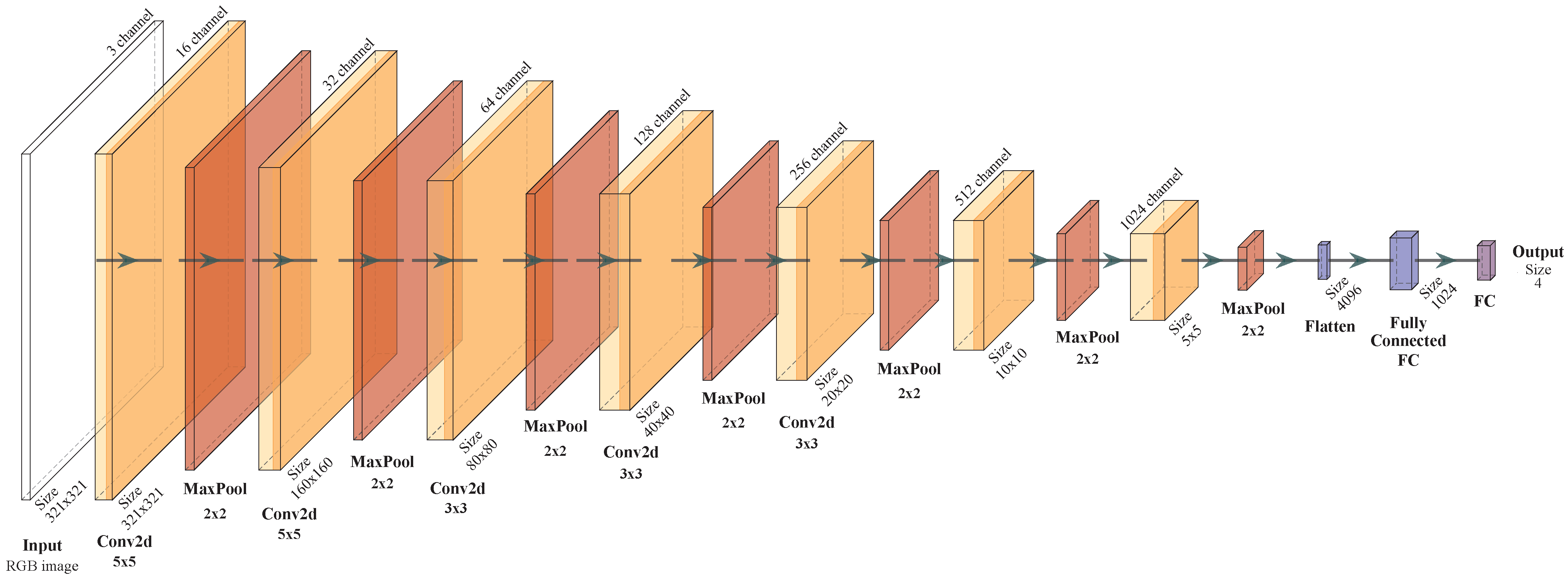
To estimate the bounding box of a target object within the extracted ROI in a scene, a deep convolutional neural network (CNN) was designed and trained. The architecture of the model is depicted in Figure A2. The input to the network is a three-channel RGB ROI image of size 321 × 321 pixels, and the output is a four-element vector y = [ x ^ c , y ^ c , w ^ , h ^ ] T corresponding to the predicted bounding box. Here, ( x c , y c ) represents the coordinates of the upper-left corner of the bounding box, and w and h denote its width and height, respectively.
The model is structured with seven convolutional layers. Each layer applies batch normalization, a ReLU activation function, and max-pooling to progressively extract robust features from the input image. The resulting feature maps are flattened into a one-dimensional vector and passed through a dropout layer with a rate of 0.2 to mitigate overfitting. The resulting feature vector is processed by a fully connected layer with 1024 neurons and mapped to an output layer with four neurons, which correspond to the estimated bounding box parameters.
The dataset used for training consists of 37,460 RGB image fragments of size 321 × 321 pixels, extracted from the LASOT (26,222 frames) and UAV123 (11,238 frames) datasets. These images are distributed across nineteen object categories considering targets with varying sizes, appearances, and background complexity to promote generalization. Each training image includes an annotated bounding box encoded as a four-dimensional vector of the form y = [ x c , y c , w , h ] T , where ( x c , y c ) denotes the coordinates of the upper-left corner, and w and h represent the width and height, respectively.
The model was trained using the Adam optimizer with a learning rate of 0.001 , and the Smooth L1 loss function, which combines the advantages of mean squared error and absolute error to improve robustness to outliers. Training was conducted over 55 epochs using mini-batch stochastic gradient descent with a batch size of 32. Model accuracy was evaluated using the Intersection over Union (IoU) metric, which compares the predicted and ground-truth bounding boxes. A prediction was considered correct if its IoU exceeded a threshold of 0.5. The trained model achieved an accuracy of 93.2%, confirming its ability to accurately estimate target bounding boxes under diverse tracking conditions.
Figure A2. Architecture of the convolutional neural network (CNN) designed for bounding box estimation.
Applsci 15 11406 g0a2

Appendix B. Drift Correction Method

In visual object tracking, drift occurs from the gradual misalignment of the tracking template with respect to the actual target in the scene. To mitigate this effect, we propose a drift correction mechanism based on a local search strategy aimed at maximizing a composite similarity score. This score is designed to guide alignment with a reference template of the true target, discourage similarity with false templates (distractors), and penalize off-centered configurations through edge-based constraints.
Let T in be the current input template, T ref the reference template of the target, and T false a template representing background or distractor content. The goal is to estimate a spatial shift ( Δ x , Δ y ) that best aligns T in with T ref while suppressing alignment with T false .
For each candidate shift ( δ x , δ y ) within a fixed window δ x , δ y [ 5 , 5 ] , the shifted version T in δ is computed using image warping. A composite score S ( δ x , δ y ) is defined as
S ( δ x , δ y ) = S true α S false β P edge .
Here, S true denotes the similarity between T in δ and T ref , and S false denotes the similarity between T in δ and T false . Misalignment errors reduce the similarity score. The similarity is computed as the correlation between normalized RGB histograms (24 bins per channel). In addition, P edge is an edge regularizer that penalizes off-center alignment, and α , β 0 are trade-off weights.
The edge penalty term P edge is computed from the shifted template as follows:
P edge = 1 Z ( i , j ) Ω edge G ( i , j ) · T in δ ( i , j ) ,
where Ω edge denotes the set of edge pixels near the template border, G ( i , j ) is a Gaussian weighting function, Z is a normalization constant, ∇ denotes the spatial gradient with respect to ( i , j ) , and · is the Euclidean norm.
The final drift correction is computed as follows:
( Δ x , Δ y ) = arg max ( δ x , δ y ) S ( δ x , δ y ) .
The correction is only applied if the resulting template exceeds a predefined similarity threshold with the current reference, ensuring robustness against incorrect corrections.
This simple method allows for correcting template drift during tracking by incorporating appearance similarity, distractor rejection, and spatial regularization.

Appendix C. Tracking Reinitialization

To recover from unexpected tracking failures, a reinitialization method based on appearance descriptors was developed. This method employs a sliding window approach over the scene to identify the region that best matches the target appearance.
During normal tracking, the algorithm maintains two sets of templates over the past N t frames: a true-class set T = { T i ( x , y ) : i = 1 , , N t } , consisting of views of the correctly detected target, and a false-class set F = { F j ( x , y ) : j = 1 , , N f } , containing fragments of false objects or background. For feature extraction, each template I ( x , y ) (either T i ( x , y ) or F j ( x , y ) ) in the set S = T F is processed to compute two key descriptors. The first is the Histogram of Oriented Gradients (HOG), defined as follows:
ϕ H ( I ( x , y ) ) R d ,
which encodes the local distribution of gradient orientations over the spatial domain of the template, thereby capturing its shape and edge structure. The dimensionality d depends on the configuration parameters of the descriptor, such as block size, cell size, and the number of orientation bins [38]. The second descriptor is the color histogram,
ϕ C ( I ( x , y ) ) R m ,
which encodes the color distribution of the template in the perceptually motivated HSV (Hue, Saturation, Value) color space. The dimensionality m is determined by the number of bins used across the selected color channels. These descriptors serve as compact and discriminative representations of target and background appearance for subsequent matching.
Let f i ( x , y ) denote the i-th captured frame of the scene. A rectangular fragment centered at ( τ x , τ y ) with width N w and height N h can be extracted from f i ( x , y ) as follows:
w τ x , τ y ( x , y ) = f i ( x , y ) · rect x τ x N w , y τ y N h ,
where rect ( · , · ) denotes the two-dimensional rectangle function, which equals 1 within the window region and 0 elsewhere. For each fragment w τ x , τ y ( x , y ) of the scene, both descriptors ϕ H ( w τ x , τ y ) and ϕ C ( w τ x , τ y ) are also computed. Therefore, a similarity score for each window position ( τ x , τ y ) is computed as follows:
sim ( τ x , τ y ) = 1 α · d hog true ( τ x , τ y ) + ( 1 α ) · d hist true ( τ x , τ y ) α · d hog false ( τ x , τ y ) + ( 1 α ) · d hist false ( τ x , τ y ) ,
where α ( 0 , 1 ) is a weighting parameter, and
d hog true ( τ x , τ y ) = min T i T CS ( ϕ H ( w τ x , τ y ) , ϕ H ( T i ) ) , d hog false ( τ x , τ y ) = min F j F CS ( ϕ H ( w τ x , τ y ) , ϕ H ( F j ) ) , d hist true ( τ x , τ y ) = min T i T CS ( ϕ C ( w τ x , τ y ) , ϕ C ( T i ) ) , d hist false ( τ x , τ y ) = min F j F CS ( ϕ C ( w τ x , τ y ) , ϕ C ( F j ) ) ,
are the minimum Cosine Similarity (CS) values between the fragment w τ x , τ y and the archived templates T i and F j considering both HOG and color descriptors. This ensures that windows similar to the target and dissimilar to background patterns receive higher scores. Finally, the coordinates of the most likely target location in the scene are estimated as follows:
( x ^ t , y ^ t ) = arg max ( τ x , τ y ) sim ( τ x , τ y ) ,
and the corresponding fragment w x ^ t , y ^ t ( x , y ) is selected as the new target template. This template best matches the accumulated appearance and shape features of the target while minimizing false detections.

References

  1. Zhao, G.; Meng, F.; Yang, C.; Wei, H.; Zhang, D.; Zheng, Z. A review of object tracking based on deep learning. Neurocomputing 2025, 651, 130988. [Google Scholar] [CrossRef]
  2. Yilmaz, A.; Javed, O.; Shah, M. Object tracking: A survey. ACM Comput. Surv. 2006, 38, 13-es. [Google Scholar] [CrossRef]
  3. Smeulders, A.W.M.; Chu, D.M.; Cucchiara, R.; Calderara, S.; Dehghan, A.; Shah, M. Visual tracking: An experimental survey. IEEE Trans. Pattern Anal. Mach. Intell. 2014, 36, 1442–1468. [Google Scholar]
  4. Wu, Y.; Lim, J.; Yang, M.H. Object Tracking Benchmark. IEEE Trans. Pattern Anal. Mach. Intell. 2015, 37, 1834–1848. [Google Scholar] [CrossRef] [PubMed]
  5. Diaz-Ramirez, V.H.; Picos, K.; Kober, V. Target tracking in nonuniform illumination conditions using locally adaptive correlation filters. Opt. Commun. 2014, 323, 32–43. [Google Scholar] [CrossRef]
  6. Ciaparrone, G.; Luque Sánchez, F.; Tabik, S.; Troiano, L.; Tagliaferri, R.; Herrera, F. Deep learning in video multi-object tracking: A survey. Neurocomputing 2020, 381, 61–88. [Google Scholar] [CrossRef]
  7. Ross, D.A.; Lim, J.; Lin, R.S.; Yang, M.H. Incremental learning for robust visual tracking. Int. J. Comput. Vis. 2008, 77, 125–141. [Google Scholar] [CrossRef]
  8. Danelljan, M.; Hager, G.; Khan, F.S.; Felsberg, M. Discriminative Scale Space Tracking. IEEE Trans. Pattern Anal. Mach. Intell. 2017, 39, 1561–1575. [Google Scholar] [CrossRef]
  9. Yang, T.; Chan, A.B. Visual Tracking via Dynamic Memory Networks. IEEE Trans. Pattern Anal. Mach. Intell. 2021, 43, 360–374. [Google Scholar] [CrossRef]
  10. Dong, X.; Shen, J.; Porikli, F.; Luo, J.; Shao, L. Adaptive Siamese Tracking with a Compact Latent Network. IEEE Trans. Pattern Anal. Mach. Intell. 2023, 45, 8049–8062. [Google Scholar] [CrossRef] [PubMed]
  11. Babenko, B.; Yang, M.H.; Belongie, S. Robust Object Tracking with Online Multiple Instance Learning. IEEE Trans. Pattern Anal. Mach. Intell. 2011, 33, 1619–1632. [Google Scholar] [CrossRef]
  12. Hare, S.; Golodetz, S.; Saffari, A.; Vineet, V.; Cheng, M.M.; Hicks, S.L.; Torr, P.H. Struck: Structured Output Tracking with Kernels. IEEE Trans. Pattern Anal. Mach. Intell. 2016, 38, 2096–2109. [Google Scholar] [CrossRef] [PubMed]
  13. Kalal, Z.; Mikolajczyk, K.; Matas, J. Tracking-Learning-Detection. IEEE Trans. Pattern Anal. Mach. Intell. 2012, 34, 1409–1422. [Google Scholar] [CrossRef]
  14. Bolme, D.S.; Beveridge, J.R.; Draper, B.A.; Lui, Y.M. Visual Object Tracking Using Adaptive Correlation Filters. In Proceedings of the IEEE Conference on Computer Vision and Pattern Recognition (CVPR), San Francisco, CA, USA, 13–18 June 2010; pp. 2544–2550. [Google Scholar]
  15. Gaxiola, L.N.; Diaz-Ramirez, V.H.; Tapia, J.J.; García-Martínez, P. Target tracking with dynamically adaptive correlation. Opt. Commun. 2016, 365, 140–149. [Google Scholar] [CrossRef]
  16. Henriques, J.F.; Caseiro, R.; Martins, P.; Batista, J. High-speed tracking with kernelized correlation filters. IEEE Trans. Pattern Anal. Mach. Intell. 2015, 37, 583–596. [Google Scholar] [CrossRef]
  17. Danelljan, M.; Hager, G.; Shahbaz Khan, F.; Felsberg, M. Learning spatially regularized correlation filters for visual tracking. In Proceedings of the IEEE International Conference on Computer Vision, Santiago, Chile, 7–13 December 2015; pp. 4310–4318. [Google Scholar]
  18. Zhang, J.; He, Y.; Wang, S. Learning Adaptive Sparse Spatially-Regularized Correlation Filters for Visual Tracking. IEEE Signal Process. Lett. 2023, 30, 11–15. [Google Scholar] [CrossRef]
  19. Danelljan, M.; Häger, G.; Khan, F.S.; Felsberg, M. Adaptive Decontamination of the Training Set: A Unified Formulation for Discriminative Visual Tracking. In Proceedings of the 2016 IEEE Conference on Computer Vision and Pattern Recognition (CVPR), Las Vegas, NV, USA, 27–30 June 2016; pp. 1430–1438. [Google Scholar]
  20. Sheng, X.; Liu, Y.; Liang, H.; Li, F.; Man, Y. Robust Visual Tracking via an Improved Background Aware Correlation Filter. IEEE Access 2019, 7, 24877–24888. [Google Scholar] [CrossRef]
  21. Zhang, J.; Yuan, T.; He, Y.; Wang, J. A background-aware correlation filter with adaptive saliency-aware regularization for visual tracking. Neural Comput. Appl. 2022, 34, 6359–6376. [Google Scholar] [CrossRef]
  22. Li, F.; Tian, C.; Zuo, W.; Zhang, L.; Yang, M.H. Learning Spatial-Temporal Regularized Correlation Filters for Visual Tracking. In Proceedings of the IEEE Computer Society Conference on Computer Vision and Pattern Recognition, Salt Lake City, UT, USA, 18–23 June 2018; pp. 4904–4913. [Google Scholar]
  23. Kumar, B.V.K.V.; Mahalanobis, A.; Juday, R.D. Correlation Pattern Recognition; Cambridge University Press: Cambridge, UK, 2005. [Google Scholar]
  24. Vijaya Kumar, B.; Hassebrook, L. Performance measures for correlation filters. Appl. Opt. 1990, 29, 2997–3006. [Google Scholar] [CrossRef]
  25. Yaroslavsky, L. The theory of optimal methods for localization of objects in pictures. Prog. Opt. 1993, 32, 145–201. [Google Scholar]
  26. Javidi, B.; Wang, J. Design of filters to detect a noisy target in nonoverlapping background noise. J. Opt. Soc. Am. A 1994, 11, 2604–2612. [Google Scholar] [CrossRef]
  27. Javidi, B.; Parchekani, F.; Zhang, G. Minimum-mean-square-error filters for detecting a noisy target in background noise. Appl. Opt. 1996, 35, 6964–6975. [Google Scholar] [CrossRef] [PubMed]
  28. Javidi, B.; Wang, J. Optimum filter for detecting a target in multiplicative noise and additive noise. J. Opt. Soc. Am. A 1997, 14, 836–844. [Google Scholar] [CrossRef]
  29. Kober, V.; Campos, J. Accuracy of location measurement of a noisy target in a nonoverlapping background. J. Opt. Soc. Am. A 1996, 13, 1653–1666. [Google Scholar] [CrossRef]
  30. Ouerhani, Y.; Jridi, M.; Alfalou, A.; Brosseau, C. Optimized pre-processing input-plane GPU implementation of an optical face recognition technique using a segmented phase-only composite filter. Opt. Commun. 2013, 289, 33–44. [Google Scholar] [CrossRef]
  31. Maragos, P. Optimal morphological approaches to image matching and object detection. In Proceedings of the 1988 Second International Conference on Computer Vision, Tampa, FL, USA, 5–8 December 1988; IEEE Computer Society: Washington, DC, USA, 1988; pp. 695–696. [Google Scholar]
  32. Martinez-Diaz, S.; Kober, V.I. Nonlinear synthetic discriminant function filters for illumination-invariant pattern recognition. Opt. Eng. 2008, 47, 067201. [Google Scholar] [CrossRef]
  33. Diaz-Ramirez, V.H.; Gonzalez-Ruiz, M.; Kober, V.; Juarez-Salazar, R. Stereo Image Matching Using Adaptive Morphological Correlation. Sensors 2022, 22, 9050. [Google Scholar] [CrossRef]
  34. Fan, H.; Bai, H.; Lin, L.; Yang, F.; Chu, P.; Deng, G.; Yu, S.; Harshit; Huang, M.; Liu, J.; et al. LaSOT: A High-quality Large-scale Single Object Tracking Benchmark. Int. J. Comput. Vis. 2021, 129, 439–461. [Google Scholar] [CrossRef]
  35. Huang, L.; Zhao, X.; Huang, K. GOT-10k: A Large High-Diversity Benchmark for Generic Object Tracking in the Wild. IEEE Trans. Pattern Anal. Mach. Intell. 2021, 43, 1562–1577. [Google Scholar] [CrossRef]
  36. Mueller, M.; Smith, N.; Ghanem, B. A Benchmark and Simulator for UAV Tracking. In Proceedings of the Computer Vision—ECCV 2016, Amsterdam, The Netherlands, 11–14 October 2016; Leibe, B., Matas, J., Sebe, N., Welling, M., Eds.; Springer: Cham, Switzerland, 2016; pp. 445–461. [Google Scholar]
  37. Rong Li, X.; Jilkov, V. Survey of maneuvering target tracking. Part I. Dynamic models. IEEE Trans. Aerosp. Electron. Syst. 2003, 39, 1333–1364. [Google Scholar] [CrossRef]
  38. Dalal, N.; Triggs, B. Histograms of Oriented Gradients for Human Detection. In Proceedings of the IEEE Computer Society Conference on Computer Vision and Pattern Recognition (CVPR), San Diego, CA, USA, 20–25 June 2005; pp. 886–893. [Google Scholar]
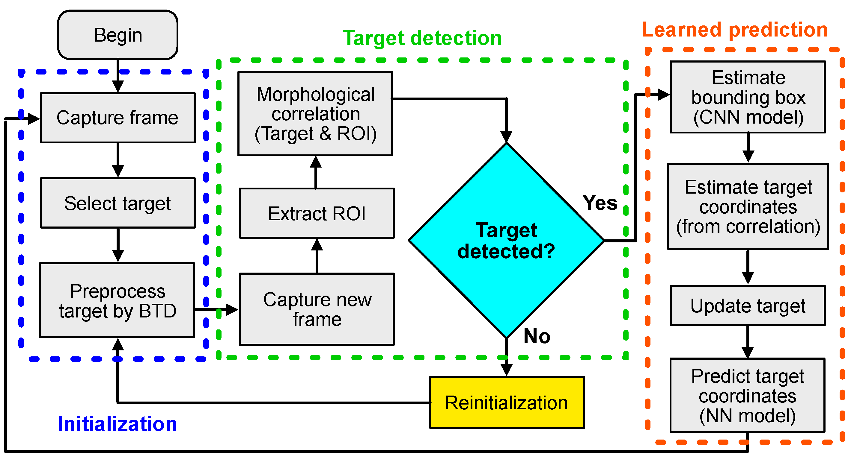
Figure 1. Flowchart of the proposed morphological-correlation-based tracking method.
Applsci 15 11406 g001
Figure 2. Representative scene frames used for target tracking from the evaluated datasets: (a) GOT-10k, (b) LaSOT, (c) OTB50, and (d) UAV123. The bounding box colors indicate the tracking results of different methods: GT (white), MCF (red), STRCF (blue), KCF (pink), STRDCF (green), SRDCFd (yellow), and BACF (cyan).
Applsci 15 11406 g002
Figure 3. Precision plots of the proposed MCF tracker and existing tracking methods evaluated on 40 sequences (38,484 frames) from (a) GOT-10k, (b) LaSOT, (c) OTB50, (d) UAV123, and (e) the combined dataset.
Applsci 15 11406 g003
Figure 4. Success plots of the proposed MCF tracker and existing tracking methods evaluated on 40 sequences (38,484 frames) from (a) GOT-10k, (b) LaSOT, (c) OTB50, (d) UAV123, and (e) the combined datasets.
Applsci 15 11406 g004
Table 1. Tracking performance of the proposed Morphological Correlation Filter (MCF) and existing methods on 40 sequences (38,484 frames) from the GOT-10k, LaSOT, OTB50, and UAV123 datasets. The results are presented as mean ± standard deviation for the normalized location error (NLE), intersection over union (IoU), and as a percentage for detection rate (DR).
DatasetTrackerNLEIoUDR (%)
GOT-10kSTRCF 0.018 ± 0.016 0.649 ± 0.228 70.1
BACF 0.015 ± 0.015 0.672 ± 0.216 73.4
SRDCF 0.047 ± 0.091 0.579 ± 0.299 59.7
SRDCFd 0.051 ± 0.099 0.577 ± 0.298 59.6
KCF 0.036 ± 0.065 0.463 ± 0.321 47.0
MCF 0.016 ± 0.026 0.747 ± 0.174 90.2
LaSOTSTRCF 0.033 ± 0.047 0.484 ± 0.313 51.4
BACF 0.083 ± 0.150 0.482 ± 0.303 53.5
SRDCF 0.122 ± 0.230 0.398 ± 0.296 44.7
SRDCFd 0.099 ± 0.115 0.408 ± 0.369 49.2
KCF 0.149 ± 0.182 0.163 ± 0.233 12.1
MCF 0.032 ± 0.054 0.575 ± 0.176 65.6
OTB50STRCF 0.012 ± 0.014 0.719 ± 0.152 91.7
BACF 0.016 ± 0.029 0.696 ± 0.179 90.8
SRDCF 0.016 ± 0.031 0.694 ± 0.187 87.3
SRDCFd 0.012 ± 0.012 0.706 ± 0.164 89.1
KCF 0.034 ± 0.085 0.592 ± 0.256 70.8
MCF 0.011 ± 0.013 0.703 ± 0.211 89.9
UAV123STRCF 0.008 ± 0.009 0.634 ± 0.206 74.4
BACF 0.007 ± 0.008 0.662 ± 0.168 81.7
SRDCF 0.008 ± 0.011 0.636 ± 0.193 74.5
SRDCFd 0.009 ± 0.011 0.645 ± 0.187 78.5
KCF 0.045 ± 0.078 0.408 ± 0.293 39.7
MCF 0.004 ± 0.005 0.754 ± 0.200 90.1
All datasetsSTRCF 0.017 ± 0.021 0.632 ± 0.224 71.9
BACF 0.030 ± 0.050 0.628 ± 0.216 74.8
SRDCF 0.048 ± 0.090 0.576 ± 0.243 66.5
SRDCFd 0.042 ± 0.592 0.584 ± 0.254 69.1
KCF 0.066 ± 0.102 0.406 ± 0.275 42.4
MCF 0.015 ± 0.024 0.694 ± 0.190 83.9
Disclaimer/Publisher’s Note: The statements, opinions and data contained in all publications are solely those of the individual author(s) and contributor(s) and not of MDPI and/or the editor(s). MDPI and/or the editor(s) disclaim responsibility for any injury to people or property resulting from any ideas, methods, instructions or products referred to in the content.