Image-Level Anti-Personnel Landmine Detection Using Deep Learning in Long-Wave Infrared Images

Abstract

This study proposes a simple deep learning-based framework for image-level anti-personnel landmine detection in long-wave infrared imagery. To address challenges posed by the limited size of the available dataset and the small spatial size of anti-personnel landmines within images, we integrate two key techniques: transfer learning using pre-trained vision foundation models, and attention-based multiple instance learning to derive discriminative image features. We evaluate five pre-trained models, including ResNet, ConvNeXt, ViT, OpenCLIP, and InfMAE, in combination with attention-based multiple instance learning. Furthermore, to mitigate the reliance of trained models on irrelevant features such as artificial or natural structures in the background, we introduce an inpainting-based image augmentation method. Experimental results, conducted on a publicly available “legbreaker” anti-personnel landmine infrared dataset, demonstrate that the proposed framework achieves high precision and recall, validating its effectiveness for landmine detection in infrared imagery. Additional experiments are also performed on an aerial image dataset designed for detecting small-sized ship targets to further validate the effectiveness of the proposed approach.

1. Introduction

Automatic detection of anti-personnel (AP) landmines is crucial to enhance safety, efficiency, and accuracy in demining operations [1]. Traditional manual detection methods expose personnel to significant risks and are often slow and labor-intensive. Automated systems, such as robotic vehicles [2] and drones [3], equipped with various sensors, can navigate hazardous areas without endangering human lives, thus accelerating the clearance process and reducing casualties. In addition, the automatic system working in real time can provide necessary information to detect AP landmines at the operation site instantly. These technological advances not only improve the speed and accuracy of mine detection, but also facilitate the safe reclamation of lands contaminated by AP landmines, ultimately contributing to the protection of civilians and the restoration of affected communities [4].

Various sensing and imaging equipments have been employed to detect landmines, such as traditional metal detectors, instruments that can measure the magnetic polarizability tensor of a conducting object [5], ground-penetrating radar [6,7], and optical imaging sensors [2,3]. AP landmines can be classified into two types depending on the type of constituent materials: metal AP landmines and low-metal-content AP landmines [4]. AP landmines commonly encountered in practice are plastic types [3,4]. Therefore, sensors utilizing the principle of electromagnetic field are not suitable for practical AP landmines. On the other hand, ground-penetrating radar shows promising performance to detect both metallic and non-metallic objects.

Optical imaging sensors used to detect AP landmines can be further divided into the following: hyperspectral imaging, visible imaging, and thermal infrared imaging sensors. Hyperspectral imaging sensors collect data in hundreds of narrow and contiguous spectral bands, unlike standard RGB cameras that capture only three color bands (red, green, blue). This characteristic can help distinguish AP landmines from surrounding materials (e.g., soil and vegetation) by analyzing spectral differences [8] or comparing the spectral signatures of AP landmines in the library [9]. However, simply considering spectral anomalies as AP landmines in the hyperspectral image can increase the number of false alarms. In addition, preprocessing is required to mitigate environmental effects in the detection of spectral signatures [10].

Visible imaging sensors are mainly used to detect surface AP landmines [2,11,12]. The representative of surface landmines is the scatterable landmine characterized by its small size, high composition of plastic, and easy deployment by aerial or armored vehicles [11,12]. As the resolution of visible images is generally higher than that of other optical images and the shape of scatterable landmines is prominent compared to other natural objects, the scatterable landmine can be detected in the visible image. However, the detection may fail when the scatterable landmines are heavily occluded by ground vegetation or obscured by the shadow of surrounding objects.

AP landmines and the soil in which they are buried exhibit distinct thermal properties, primarily due to differences in thermal conductivity, heat capacity, and thermal diffusivity [13]. These differences influence how heat is transferred and retained, leading to detectable thermal contrasts on the soil surface [4] crucial for detection methods that utilize thermal infrared imaging sensors. As environmental conditions such as ambient temperature, solar radiation, relative humidity, and wind speed can influence the thermal contrast [14], these factors not only should be considered in the thermal image acquisition but may also limit the use of the thermal imaging sensor in AP landmine detection. Overall, rather than solely being used, different sensing and imaging equipments can collectively contribute to configuring more reliable automated mine detection systems, improving operational effectiveness.

In this work, our focus is on developing automated detection of AP landmines in thermal infrared images. Deep learning has shown remarkable success in various computer vision applications through continuous technological advancements in various aspects. Motivated by this, we organize appropriate techniques from the recent advancements of the computer vision community so as to devise a new method that can detect AP landmines effectively. The existing literature already includes several studies that utilize deep learning techniques for detecting AP landmines in visible and thermal infrared images. In [11], visible images of scatterable AP landmines obtained from an unmanned aerial vehicle are manually annotated. Then, the well-known object detector, Faster region-based convolutional neural network (Faster R-CNN) [15], is trained to detect the scatterable AP landmines. To improve the detection performance, pre-trained ResNet101 [16] is utilized. In [12], RGB and near-infrared images are firstly fused by a lightweight CNN, then Faster R-CNN detects scatterable AP landmines in the fused image. The fusion network and detector networks are simultaneously trained by minimizing both the low-level task (i.e., image reconstruction) and high-level task (i.e., landmine detection) losses. In [2], a mobile camera mounted on a demining robot captures visible images. After annotating the images, YOLOv8 [17] is trained to detect two types of surface AP landmines. In contrast to works that automatically detect AP landmines in visible images, most research on detecting AP landmines in thermal infrared images relies on classical human-designed detection methods [3,4,18,19]. One notable exception is the study in [20], where a binary CNN classifier and the YOLOv8 object detector are explored. In the work, the binary classifier is trained to determine the presence of AP landmines in an input image, while YOLOv8 is trained to localize their positions.

On the contrary to most previous studies that focus on localizing AP landmines in the input image, we propose a deep learning-based method that can output whether AP landmines exist in the input image. The motivation behind our choice of image-level detection is twofold. First, the dataset [14] used in this work provides only image-level labels. The study in [20] also utilizes the same dataset [14], where the authors manually annotated regions containing AP landmines and used these annotations to train an AP landmine detection model. However, in some cases, AP landmines are only partially visible due to vegetation, making it difficult to accurately annotate the regions containing them. This ambiguity can result in inconsistent labels, which may ultimately degrade the performance of the detection model [21]. The second reason is that if satisfactory performance can be achieved using only the presence information of AP landmines within an image, the cost and time required for annotating the collected images can be significantly reduced.

The remainder of this paper is organized as follows. Section 2 briefly describes the dataset [14] used in this work and presents an analysis of it. Based on the insights gained from our examination, we present key solutions to the addressed problems in Section 3. Experimental results are reported in Section 4, and the conclusions are drawn in Section 5.

2. Dataset

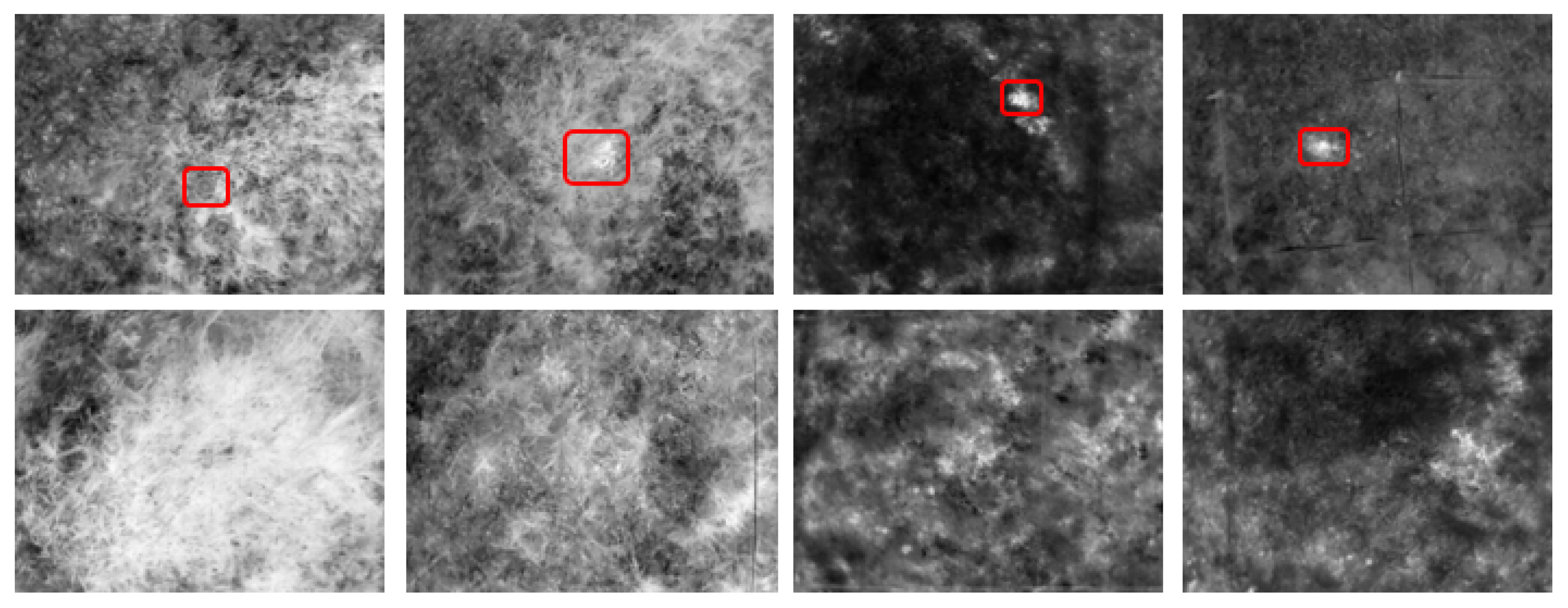
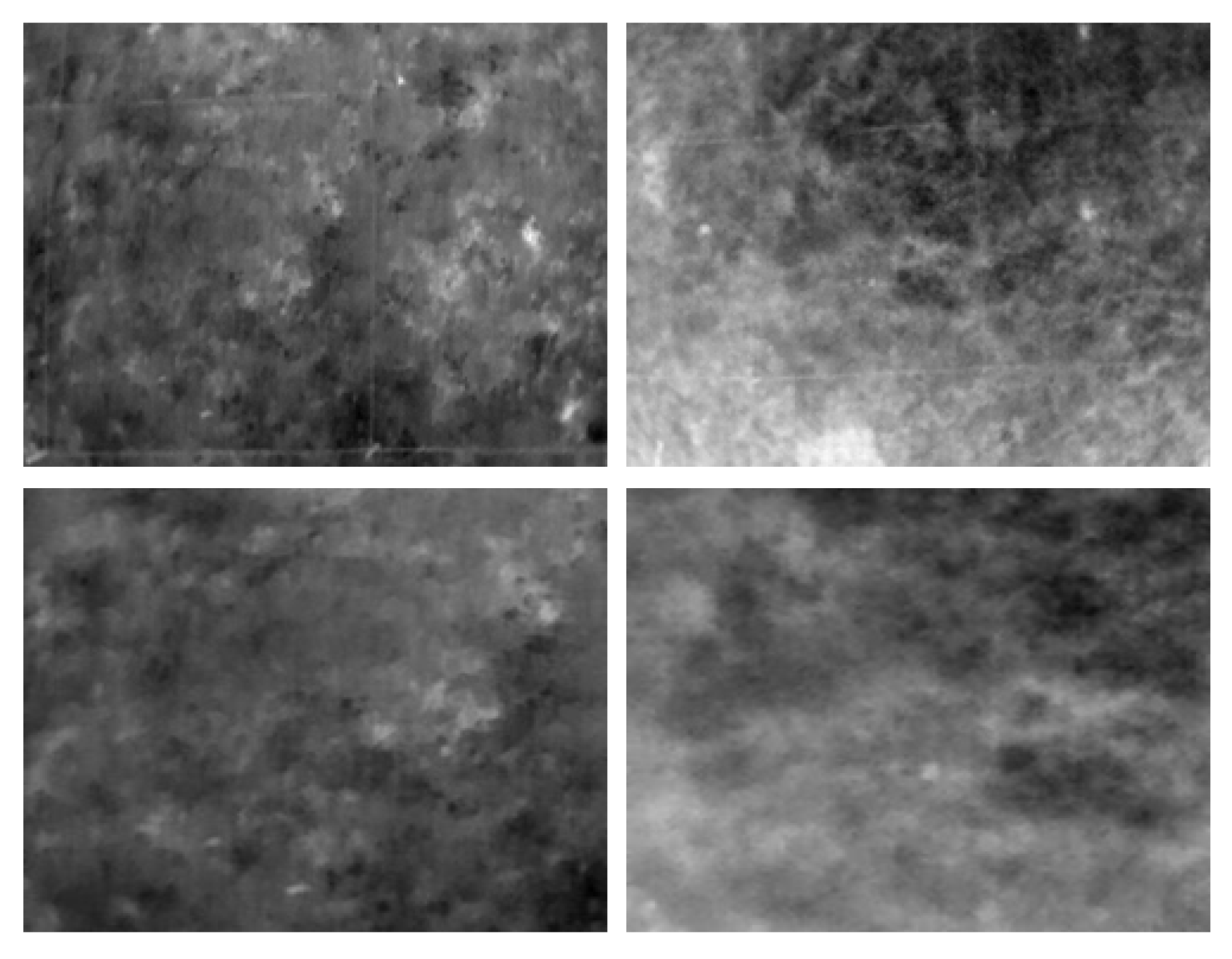
2.1. AP Landmine Dataset

A publicly available dataset for the detection of “legbreaker” AP landmines [3,14] is selected in this work. Although another dataset exists for AP landmine detection experiments [4], it was constructed using homogeneous terrain, which may cause experimental results obtained from it to differ significantly from those encountered in real-world field inspections [3]. To construct the dataset, authors of [3] produced eight replicas of AP landmines used by armed groups in Colombia. The replica measures 8.7 cm in diameter and 10.2 cm in height. The replicas were installed on a square soil area of 10 m side approximately with scarce vegetation [3]. The area was divided into nine zones, with AP landmine replicas buried at depths of 0, 1, 5, and 10 cm in eight of them. The remaining zone was left free of AP landmines. Thermographic images of the nine zones were captured using a DJI Zenmuse XT camera (DJI, Shenzhen, China), operating in the spectral range of 7.5 to 13.5 $\mathsf{\mu }$m, mounted on a DJI Matrice 100 unmanned aerial vehicle (DJI) (UAV) [3]. For each zone, the altitude of the UAV was gradually decreased from 10 to 1 m in one meter decrements to capture images of AP landmines at varying apparent sizes. Some example images of the dataset are given in Figure 1.

Images of the dataset are provided in three formats: JPG, TIFF, and R-JPG. The R-JPG format was selected for our analysis and experiments as its image resolution (336 × 256) matches the pixel count of the infrared camera specified in [3]. The following metadata is given along with each image: date of image acquisition, flight altitude of the UAV at the time of image acquisition, central temperature of the image, and the zone number indicating the presence and depth of AP landmines. Therefore, we label images as positive if the zone number belongs to one of the eight zones where AP landmines were buried, and as negative otherwise. The images in the dataset are utilized without any preprocessing, with a single exception. When the UAV operates at a high altitude over a landmine-free zone, the infrared camera captures portions of adjacent AP landmine-contaminated areas in addition to the intended landmine-free region. To prevent discrepancies between the label information and the corresponding input image, only the landmine-free regions are cropped from the mixed images. Accordingly, we thoroughly examined the negative images to identify any mixed captures and manually cropped the landmine-free regions from all such images. Figure 2 shows examples of the mixed image and the cropped landmine-free image.

The dataset comprises 659 images, including 68 landmine-free (negative) images and 591 AP landmine (positive) images. This reflects (1) a significant class imbalance that may adversely affect the training process and (2) a limited overall dataset size, which results in variations in the performance evaluation of the model depending on the train–test split. A simple and widely used approach to address class imbalance is oversampling, which involves increasing the number of underrepresented class samples using techniques such as sample duplication [22]. Therefore, we simply duplicate the negative samples so as to match the number of negative samples with that of the positive samples in the training phase only. Before duplicating the negative samples, we split the dataset into the training and test sets by preserving the ratio of the negative and positive samples in the original dataset.

To address the problem of performance variations and evaluate the generalization performance of the trained model, we employ k-fold cross-validation, a widely adopted technique in the literature [23,24] when working with small-sized datasets. In k-fold cross-validation, the dataset is partitioned into k equally sized subsets or folds. The model is then trained and validated k times, each time using a different fold as the test set while the remaining $k-1$ folds are used for training. The final evaluation results are obtained by averaging the k individual results or accumulating those. This ensures that a performance measure of the trained model is less sensitive to the variability of a single train–test split. In our work, k is set to 5. It is important to note, however, that k-fold cross-validation cannot fully mitigate the limitations imposed by the small size of the dataset. In other words, the restricted dataset size may still hinder the model from achieving optimal classification performance.

Another distinguishing characteristic of the dataset is the relatively small size of AP landmines within the images. Unlike conventional image classification datasets such as ImageNet [25] where objects of interest typically occupy a significant portion of the image, AP landmines cover only a small area, as shown in Figure 1. As a result, when a global pooling operation—commonly used to obtain image-level features—is applied to the extracted feature maps, the resulting feature tends to be dominated by background information. This dominance can suppress the discriminative features associated with AP landmines.

In Section 3, we present our approach to addressing the key challenges that hinder model performance, namely, the limited size of the dataset and the small spatial footprint of AP landmines within the images.

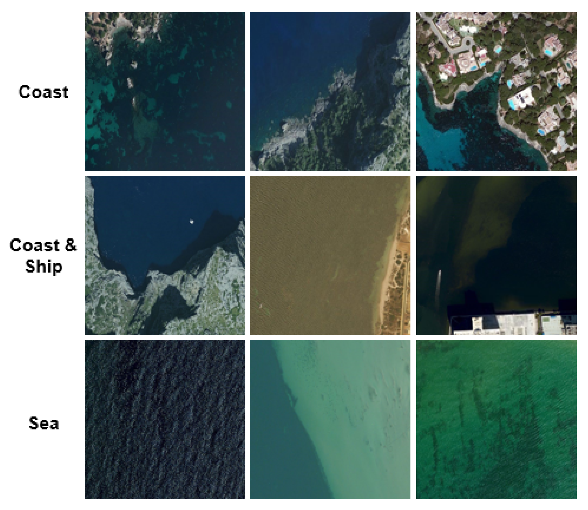
2.2. MASATI (MAritime SATellite Imagery) Dataset

Another public dataset called MASATI [26] is used in our experiments to assess the effectiveness of the proposed approach. The MASATI dataset was initially constructed for the classification of scenes with ships in satellite RGB images [27]. Then, the dataset was extended for the detection of ships [28,29] by increasing the number of images and providing ship location annotations. The spatial resolution of images is $512\times 512$ and the length of each ship spans from 20 to 100. Despite differences in spectral range and partial occlusion of objects compared to our primary dataset, the MASATI dataset shares key characteristics such as small target size and off-center object placement. This makes the MASATI dataset suitable for validating our AP landmine classification framework. Among seven classes in the MASATI dataset, we select three for our study: “Coast”, “Coast & ship”, and “Sea”. Each class contains approximately 1000 samples. Images from the first two classes are used to train models for binary classification, distinguishing between the presence and absence of ships. This task closely resembles image-level AP landmine detection, where the model learns to make a binary decision regarding the presence of a small, off-center AP landmine in the image. The role of the third class will be discussed in Section 4. Example images from all three classes are shown in Figure 3.

3. Methods

3.1. Transfer Learning

Existing studies have shown that increasing both the diversity and quantity of training samples together with the model capacity can improve the performance of trained models [30]. For applications like ours, where the cost and effort to collect a sufficient number of training samples are unaffordable, this approach is not feasible. By leveraging the transfer learning technique, the pre-training, fine-tuning, and prediction paradigm [31], the problem of the small-sized dataset can be overcome. In this approach, a model is initially pre-trained on a large-scale dataset to learn general representations and is subsequently fine-tuned on a smaller, task-specific dataset to adapt to the target application. Depending on the availability of labels in the pre-training dataset, pre-training can be categorized as either supervised or self-supervised. The representative example of a supervised pre-training model is a CNN trained on the ImageNet [25] dataset with a supervised loss. However, supervised pre-training relies on large-scale labeled data for pre-training, which can limit the scalability of the dataset and hinder the learning of more powerful features. The recent advances in self-supervised learning [32,33] show that useful and transferable representations can be learned without labels. As self-supervised pre-training can cope well with the scalability of training sample sizes, it even shows better performance in downstream tasks compared to supervised pre-training [34].

Advantages of utilizing pre-trained models for downstream tasks can be summarized as follows. First, pre-trained models can be applied across a wide range of downstream tasks, making them highly versatile. Second, they enable significantly improved performance using only a small amount of annotated data, compared to training models from scratch. Most importantly for our work, even in the presence of a substantial domain gap between the pre-training and fine-tuning datasets, pre-trained models can still enhance downstream task performance through adaptation. Notable examples include land cover classification from remotely sensed images [35] and fault classification of solar modules using infrared imagery [36], both of which have successfully employed ImageNet pre-trained models.

These advantages naturally lead us to leverage pre-trained models to cope with a limited number of the AP landmine dataset. In this work, a total of five pre-trained models are explored. A summary of models employed in this work is given in

Table 1. A summary of models employed in this work and some key features of the dataset used to perform pre-training.

Model	Backbone	# of Param.(M)	Dataset	Sup./Self.	Modality
ResNet [16]	ResNet50	23.5	IN1K	sup.	image
ConvNeXt [38]	ConvNext-Base	87.6	IN21K	sup.	image
ViT [39]	ViT-Base	102.6	IN21K	sup.	image
OpenCLIP [40]	ViT-Base	86.6	LAION400M	self.	image–text pair
InfMAE [41]	ConvViT-Base	89.1	Inf30	self.	infrared image

. The first pre-trained model is the residual network (ResNet) [16] learned on the ImageNet1K (IN1K) dataset [25]. The distinct characteristic of ResNet compared to previous CNN models is the residual block architecture, which incorporates identity shortcut connections that bypass one or more layers. Instead of directly learning a desired underlying mapping $H\left(x\right)$, residual blocks are designed to learn a residual function $F\left(x\right)=H\left(x\right)-x$. This architecture facilitates the flow of gradients during backpropagation, effectively addressing the vanishing gradient problem and enabling the successful training of networks with substantially increased depth [16]. Due to its robustness and ease of optimization, ResNet models have been utilized in various domain-specific applications such as remote sensing [35] and medical image analysis [37].

The second model we investigate is ConvNeXt [38] pre-trained on the ImageNet21K (IN21K) [25], a modernized CNN inspired by Vision Transformers (ViTs). ConvNeXt is designed to narrow the performance gap between CNN models and ViT models while preserving the efficiency and inductive biases inherent to convolutions [38]. ConvNeXt incorporates several architectural refinements borrowed from ViT [42]. Specifically, the standard convolutions are replaced by depthwise separable convolutions having a large kernel size (7 × 7) to improve computational efficiency and performance. Inverted bottleneck blocks, a design borrowed from MobileNetV2 [43] are used to enhance feature transformation. Various modifications to micro-design such as replacing ReLU with GeLU and substituting batch normalization with layer normalization are also introduced. Simulation results of ConvNeXt pre-trained on a large dataset show that the modernized CNN models are not inferior compared to ViT models [38].

The third pre-trained model is ViT [39] trained on the ImageNet21K [25] dataset. Unlike CNN models that rely on localized receptive fields and hierarchical feature extraction, ViT treats an image as a sequence of fixed-size non-overlapping patches and processes them using a transformer encoder. In ViT, the non-overlapping patches is linearly embedded into a fixed-dimensional vector. These patch embeddings are combined with positional encodings to retain spatial information and then passed through multiple transformer layers consisting of multi-head self-attention and feedforward sub-layers. One of the key advantages of ViT is its ability to model long-range dependencies across the entire image using self-attention mechanisms, enabling more global feature representations [44]. However, its performance heavily depends on large-scale pre-training, as it lacks the inductive biases inherent in CNN models [39].

OpenCLIP [40] designed to facilitate scalable multi-modal (text-image pair) learning using publicly available datasets such as LAION-400M and LAION-2B [45] is also inspected for our task of interest. OpenCLIP adopts a dual-encoder architecture consisting of a vision encoder and a transformer-based text encoder that jointly learns via contrastive loss to align image and text representations in a shared embedding space. OpenCLIP supports large-batch contrastive learning, mixed-precision learning, and an efficient distributed learning framework that allows OpenCLIP to scale to billions of image–text pairs [45]. The pre-trained model demonstrates strong zero-shot and few-shot performance across a range of vision tasks, including image classification, retrieval, and transfer learning. This makes OpenCLIP a versatile foundation model for vision-language applications. In this work, only the pre-trained vision encoder of OpenCLIP is utilized.

The final model employed in our study is InfMAE [41], a foundation model specifically designed for the infrared image modality. Inspired by the well-known self-supervised framework, Masked Autoencoder (MAE) [33], InfMAE introduces several key modifications tailored to the characteristics of infrared imagery. Notably, the original random masking strategy in MAE is replaced with an information-aware masking mechanism, which selectively masks less informative regions to better focus the learning process on semantically rich content. Additionally, the transformer-only encoder architecture of MAE is modified in InfMAE to include two convolutional stages followed by a transformer stage (ConvViT), enabling multi-scale feature extraction. A further significant contribution is the release of Inf30, a newly curated large-scale unannotated infrared dataset comprising 305,241 images that enables the pre-training of the model. InfMAE shows superior performance across several downstream tasks, including semantic segmentation, object detection, and small target detection, surpassing conventional pre-trained models in the infrared domain [41].

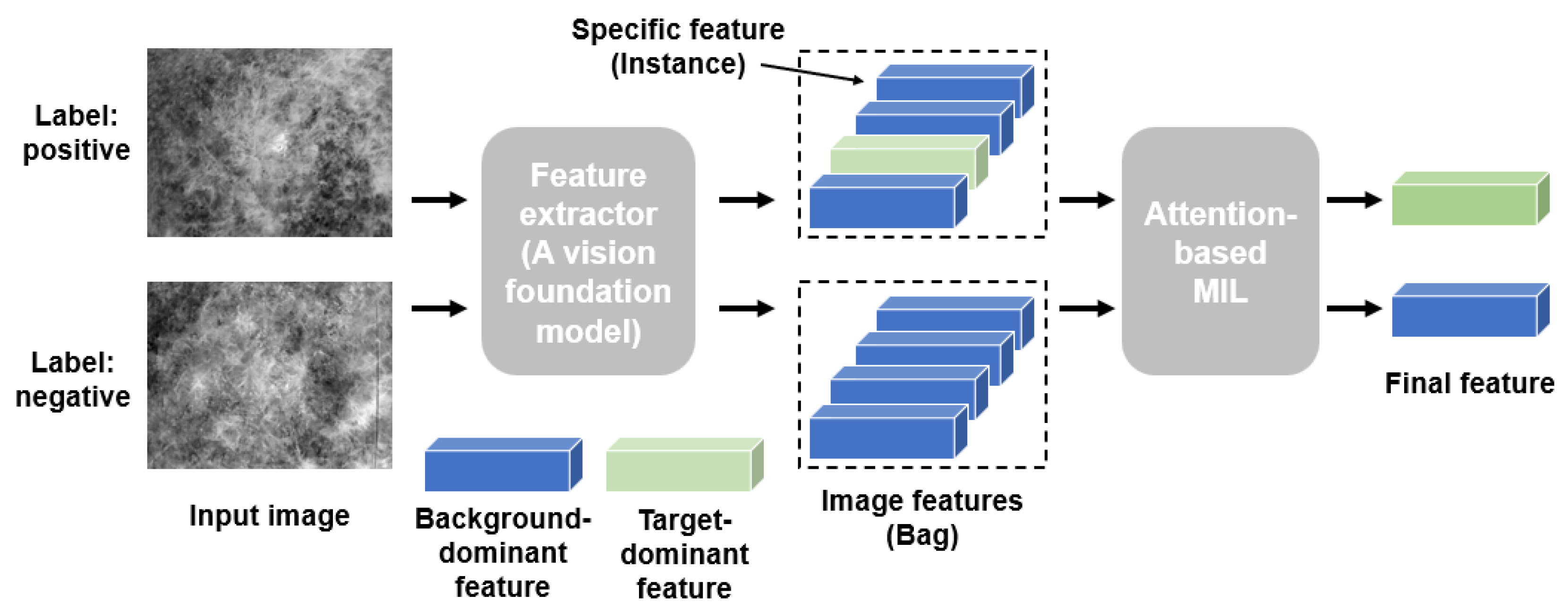
3.2. Multiple Instance Learning

Multiple instance learning (MIL) is a form of supervised learning where training data is organized into sets called bags, each containing multiple instances. In this framework, only the bag-level label is provided and labels of instances in each bag are unknown. A bag is labeled as positive if at least one of instances within the bag is positive, and negative if all instances are negative. MIL is particularly useful in scenarios where precise annotations at the instance level are expensive or impractical to obtain. By learning from incomplete labeled data, MIL enables models to identify and focus on the most informative instances within each bag, facilitating robust learning under label uncertainty.

When applying MIL to our problem, the image features extracted by the pre-trained vision foundation model can be regarded as a bag. The features corresponding to the spatial locations of AP landmines (in the case of CNN) or the patch embeddings associated with AP landmines (in the case of ViT) are treated as positive instances, as shown in Figure 4. However, we do not know which feature is associated with an AP landmine as only the image-level label is given, which implies that labels of instances are unknown. Since the number of features related to AP landmines is much smaller than that of features dominated by backgrounds, globally pooling the entire image feature may result in a suboptimal representation for classification. To address this issue, we employ an attention-based MIL (ABMIL) [46] to derive a more discriminative feature, which is then used for image-level detection.

Let us assume that N features ${\mathbf{h}}_1,{\mathbf{h}}_2,\cdots ,{\mathbf{h}}_N$ extracted by a pre-trained model are given. Each feature can be accessed by the spatial index in the case of CNN models or by the patch index in the case of ViT models. In ABMIL [46], a bag-level feature $\mathbf{z}\in {\mathbb{R}}^{D\times 1}$, i.e., an aggregation of the given instance-level N features, is calculated by

$$\mathbf{z}=\sum _{i=1}^N{a}_i{\mathbf{h}}_i,$$

(1)

where $a_i$ denotes the attention value for the ith instance ${\mathbf{h}}_i\in {\mathbb{R}}^{D\times 1}$. Ideally, the attention value should be higher for the features closely related to AP landmines, and lower or near to zero for the rest when an input image contains an AP landmine. The attention value is given by [46]

$$a_i={\displaystyle \frac{exp\left\{{\mathbf{w}}^{\mathrm{T}}\left(\tanh \left(\mathbf{V}{\mathbf{h}}_i\right)\odot \mathrm{sigm}\left(\mathbf{U}{\mathbf{h}}_i\right)\right)\right\}}{{\sum }_{j=1}^{N}exp\left\{{\mathbf{w}}^{\mathrm{T}}\left(\tanh \left(\mathbf{V}{\mathbf{h}}_j\right)\odot \mathrm{sigm}\left(\mathbf{U}{\mathbf{h}}_j\right)\right)\right\}}},$$

(2)

where $\mathbf{w}\in {\mathbb{R}}^{L\times 1}$, $\mathbf{V}\in {\mathbb{R}}^{L\times D}$, and $\mathbf{U}\in {\mathbb{R}}^{L\times D}$ are learnable parameters with hidden dimension L. ⊙ denotes element-wise multiplication. The hyperbolic tangent $\tanh \left(·\right)$ and the sigmoid non-linearity $\mathrm{sigm}\left(·\right)$ in Equation (2) are included for proper gradient flow [46] and gating mechanism [47], respectively. The final image feature $\mathbf{z}$ in Equation (1) is fed to a linear classifier to generate the classification (image-level detection) output. During fine-tuning, the parameters of the linear classifier, the ABMIL module in Equation (2), and the vision foundation model are jointly updated by minimizing the binary cross entropy loss.

3.3. Mitigating Spurious Features via Image Inpainting Augmentation

Existing studies have shown that deep image classifiers trained with a single supervision label often heavily rely on spurious background features, patterns unrelated to the target foreground, possibly leading to fault predictions based on these cues [48,49,50]. This issue is particularly prominent in both CNN-based and ViT-based ImageNet pre-trained models when the models make a prediction on the images where the size of foreground object is small and the location of foreground object is far from the center [50]. This suggests that classifiers fine-tuned on the AP landmine dataset may also strongly rely on spurious features, given that AP landmines occupy a small portion of the image and are typically not centrally located. Therefore, the trained models will not generalize well to unseen background images.

Rather than employing specialized techniques [49] to reduce reliance on spurious features in prediction results, we propose a simple image augmentation strategy inspired by a recent approach for analyzing the influence of spurious features in ImageNet pre-trained models [50]. Specifically, we first annotate bounding boxes around AP landmines in all positive images from the AP landmine dataset. It is important to note that this annotation process does not require strict guidelines or validation to minimize label noise [21]; the annotated regions need only be sufficiently large to encompass the AP landmine. The selected regions are then inpainted using the well-known image inpainting model, LaMa [51], to create synthetic landmine-free images, which are subsequently used to augment the landmine-free image set. Examples of original AP landmine images and their inpainted counterparts are shown in Figure 5. For clarity, we refer to the train set augmented by duplicating real landmine-free images (as described in Section 2) as the duplicated train set and, and the train set that includes both synthetic (i.e., inpainted version of AP landmine images in the train set) and real landmine-free images as the inpainting-augmented train set.

An additional purpose in constructing the synthetic landmine-free dataset is to enable quantitative interpretation of classification results. A common approach to model interpretability involves generating heatmaps that highlight regions most influential to the model’s predictions [52,53]. However, these methods are qualitative, require human supervision, and can be noisy, thus making their judgements potentially unreliable [48]. To complement heatmap-based interpretations, we leverage our synthetic landmine-free images for a more objective analysis. Regardless of whether the model is trained on the duplicated or inpainting-augmented train set, we can evaluate its predictions on synthetic landmine-free images that correspond to AP landmine images in the test set. Since the model has never encountered these inpainted versions during training, a high probability of positive classification suggests a strong reliance on spurious features, whereas low positive predictions imply that the model is focusing more appropriately on features related to AP landmines.

4. Experimental Results

4.1. Experimental Setup

Our experiments are conducted on an NVIDIA GeForce RTX 3090 GPU using the PyTorch framework. Models are trained using the AdamW optimizer with a weight decay of $0.05$. The initial learning rate is set to $0.0001$ and is adjusted throughout training using a cosine learning rate scheduler, with a linear warm-up over the first 10 epochs. Figure 6 shows the learning rate curve and examples of loss curves. As well as the aforementioned models in Section 3, we additionally implement the binary CNN-based classifier proposed in [20] to compare it with the proposed framework. All models are trained for 100 epochs with a batch size of 8. For ResNet, ConvNeXt, and InfMAE backbones, the spatial dimensions of the input images are preserved. In contrast, for ViT and OpenCLIP backbones, the input images are resized to $224\times 224$. For transformer-based models such as ViT, OpenCLIP, and InfMAE, the size of patch is set to $16\times 16$. For the binary CNN-based classifier, we follow the setup described by the authors in [20], where input images are resized to $256\times 256$. To further mitigate the limitations posed by the small dataset size, we apply data augmentation techniques involving geometric and photometric transformations available in the PyTorch framework. The specific data augmentation methods and associated parameters are detailed in

Table 2. Employed data augmentation methods in the Pytroch framework to augment the training images. Height and width of input images are represented by h and w, respectively.

Augmentation Method	Parameters
RandomHorizontalFlip	p = 0.5
RandomVerticalFlip	p = 0.5
RandomResizedCrop	size = (h,w),scale = (0.9, 1.0)
RandomRotation	degrees = 45
ColorJitter	brightness = 0.1, contrast = 0.1

.

To evaluate the performance of the inspected models, we employ three widely used classification metrics: precision, recall, and F1-score. Let us denote P and N as positive (images with AP landmine in it) and negative (images with no AP landmine in it), respectively. Let us also denote TP, TN, FP, and FN as correctly predicting a positive sample, correctly predicting a negative sample, incorrectly predicting a negative sample as a positive sample, and incorrectly predicting a positive sample as a negative sample, respectively. Then, precision, measuring the accuracy of positive predictions, is given by

$$\mathrm{Precision}={\displaystyle \frac{\mathrm{TP}}{\mathrm{TP}+\mathrm{FP}}}.$$

(3)

Recall, reflecting the model’s ability to correctly identify all relevant positive samples, is given by

$$\mathrm{Recall}={\displaystyle \frac{\mathrm{TP}}{\mathrm{TP}+\mathrm{FN}}}.$$

(4)

Finally, F1-score, the harmonic mean of precision and recall, is given by

$$\mathrm{F}1\text{-}\mathrm{score}={\displaystyle \frac{2\times \mathrm{Precision}\times \mathrm{Recall}}{\mathrm{Precision}+\mathrm{Recall}}}.$$

(5)

These three metrics are derived from the confusion matrix, which summarizes the classification results by recording TP, TN, FP, and FN.

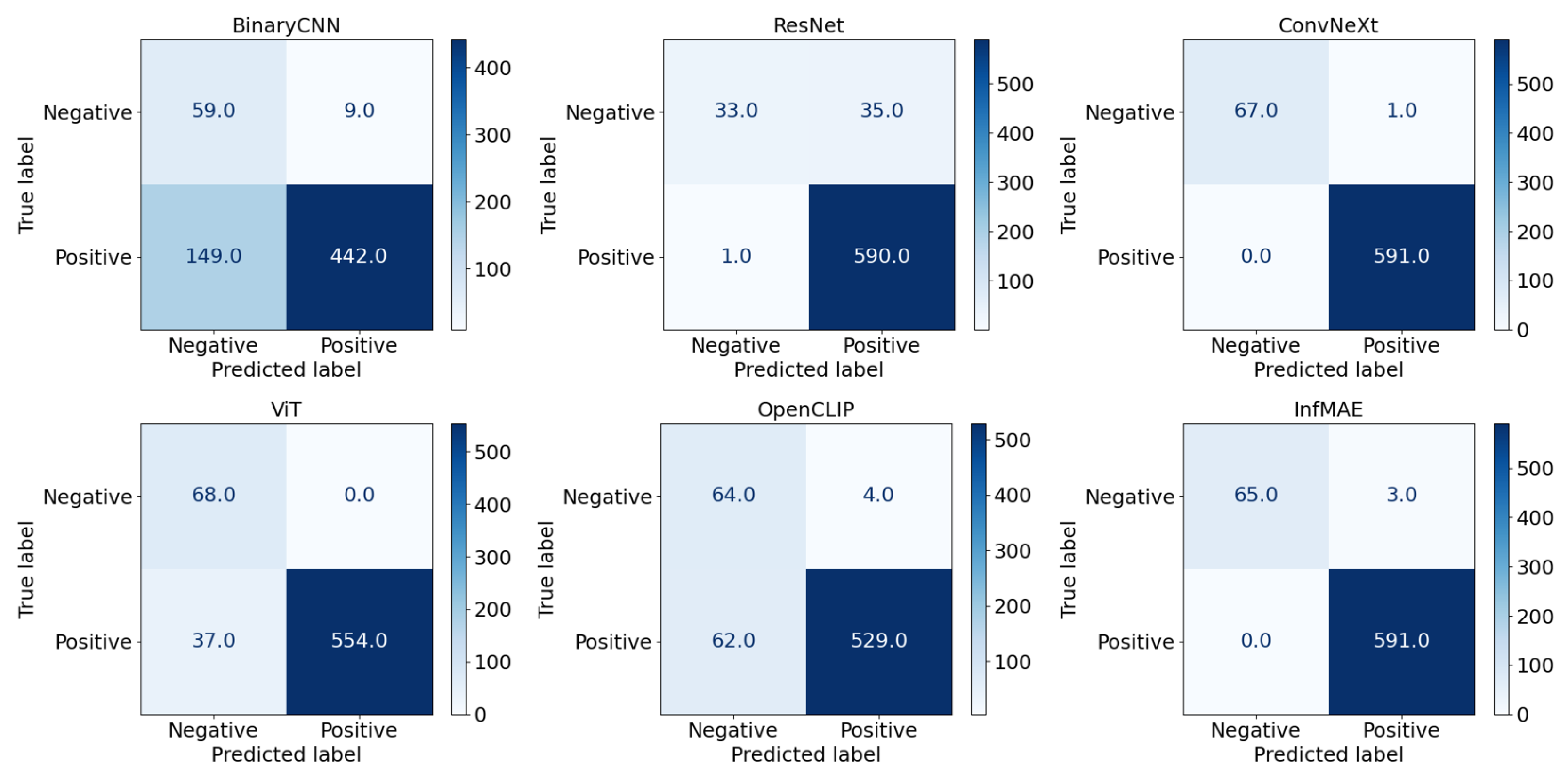
4.2. Results with Duplicated Train Set

Using the prediction results on the test set, the confusion matrices for the five foundation models and the binary CNN-based classifier are generated and presented in Figure 7. Since we perform 5-fold cross-validation, as described in Section 2, the sum of the elements in each confusion matrix equals the total number of images in the dataset. The precision, recall, and F1-score for the positive class are calculated and summarized in

Table 3. Precision, recall, and F1-score of positive class (images with AP landmine) when models are trained with the duplicated train set. The best values are highlighted in bold.

Model	BinaryCNN	ResNet	ConvNeXt	ViT	OpenCLIP	InfMAE
Precision	0.957 ± 0.004	0.989 ± 0.003	0.991 ± 0.002	0.985 ± 0.002	0.981 ± 0.004	0.987 ± 0.004
Recall	0.967 ± 0.007	0.993 ± 0.002	1.000 ± 0.000	0.998 ± 0.002	0.996 ± 0.006	0.997 ± 0.003
F1-score	0.962 ± 0.003	0.991 ± 0.001	0.995 ± 0.001	0.991 ± 0.001	0.989 ± 0.002	0.992 ± 0.003

. The first notable observation from the experimental results is that all five vision foundation models, when combined with ABMIL, achieve consistently high precision, recall, and F1-score values. The lowest precision and recall observed are $0.961$ and $0.964$, respectively, produced by the binary CNN-based classifier. Another important finding is that ConvNeXt, when combined with ABMIL, correctly classifies all positive images (i.e., recall rate is equal to 1) in the dataset. In the context of landmine detection applications, achieving a high recall rate is particularly crucial, as failing to detect positive samples could lead to serious safety risks.

We use Grad-CAM [52] to visualize the regions of input images that most influence the classification decisions of the trained models. Although visualization methods tailored specifically for ViT exist [53], we apply Grad-CAM across all model architectures to enable direct and consistent comparisons. Figure 8 presents Grad-CAM heatmaps for the five vision foundation models. From top to bottom, the size of the AP landmine in the test images progressively decreases. The heatmaps produced by ResNet closely align with the actual locations of the AP landmines. In contrast, the heatmaps for the other models generally appear unrelated to the target objects. To quantitatively assess the extent to which models rely on spurious features, we evaluate their performance on 591 synthetic landmine-free images, with the results summarized in

Table 4. Prediction results on the synthetic landmine-free images for the models trained with the duplicated train set.

Model	BinaryCNN	ResNet	ConvNeXt	ViT	OpenCLIP	InfMAE
Number of false positives	515	320	432	468	481	421

. Surprisingly, all models—even ResNet, which visually appears to attend to the foreground—produce a substantial number of false positives. This suggests a strong reliance on spurious features in their decision-making processes.

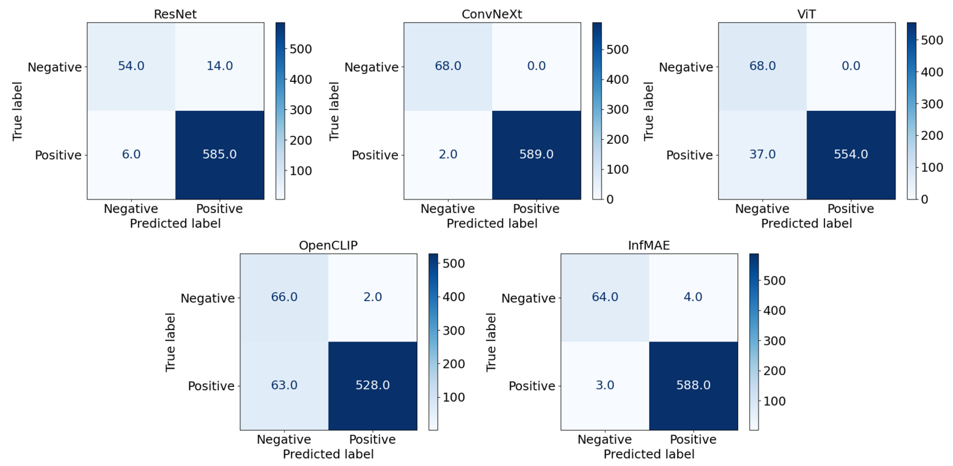
4.3. Results with Inpainting-Augmented Train Set

We repeat the same experiment like before but with the inpainting-augmented train set. Confusion matrices and the precision, recall, and F1-score for the positive class are given in Figure 9 and

Table 5. Precision, recall, and F1-score of positive class (images with AP landmine) when models are trained with the inpainting-augmented train set. The best values are highlighted in bold.

Model	BinaryCNN	ResNet	ConvNeXt	ViT	OpenCLIP	InfMAE
Precision	0.973 ± 0.009	0.933 ± 0.009	0.996 ± 0.003	1.000 ± 0.000	0.994 ± 0.004	0.990 ± 0.005
Recall	0.757 ± 0.008	0.999 ± 0.001	1.000 ± 0.000	0.928 ± 0.013	0.894 ± 0.013	1.000 ± 0.000
F1-score	0.851 ± 0.007	0.965 ± 0.004	0.998 ± 0.001	0.963 ± 0.007	0.941 ± 0.006	0.995 ± 0.002

, respectively. Notably, the classification performance of the binary CNN-based classifier, ResNet, ViT, and OpenCLIP drops compared to previous experiments. The amount of the performance drop is the largest for the binary CNN-based classifier. Only the F1-score of ConvNeXt and InfMAE increases. In addition, only the two models, ConvNeXt and InfMAE, achieve the perfect recall.

Figure 10 presents Grad-CAM heatmaps for the same original images shown in Figure 8. As before, heatmaps of ResNet remain closely aligned with the target locations. Compared to the previous results, the heatmaps for ConvNeXt and ViT now exhibit better alignment with the AP landmine regions. However, for the rest models, it remains unclear whether their predictions are primarily based on core (foreground) features. The classification results on the synthetic landmine-free images are given in

Table 6. Prediction results on the synthetic landmine-free images for the models trained with the inpainting-augmented train set.

Model	BinaryCNN	ResNet	ConvNeXt	ViT	OpenCLIP	InfMAE
Number of false positives	52	2	0	15	25	0

. A comparison between Table 4 and Table 6 reveals a substantial reduction in the number of false positives across all models. This suggests that the proposed augmentation method effectively encourages the models to focus on core features during classification. Although the qualitative evidence for InfMAE is inconclusive, its zero false positive in the quantitative evaluation supports its improved focus on meaningful features.

4.4. Ablation Studies

We firstly examine the impact of ABMIL on classification performance. In this experiment, the feature map generated by the feature extractor is reduced to a single feature vector via mean pooling, and all models are initialized with the pre-trained weights. The corresponding confusion matrices are shown in Figure 11. As illustrated in Figure 11, the number of false negatives (missing targets) increases under this setting except for ViT. The results suggest that ABMIL is better suited than the global pooling approach for this classification task. In other words, ABMIL effectively addresses the challenge posed by the small spatial footprint of AP landmines.

Finally, to evaluate the effects of transfer learning, we also conducted experiments by training all models from scratch. The resulting confusion matrices are presented in Figure 12. By comparing Figure 9 and Figure 12, we can observe that both the number of false negatives and false positives increase across all models when trained from scratch. The increase in false negatives is particularly pronounced, leading to significant declines in recall. The results indicate that transfer learning is an essential element to improve the performance of models trained from the limited number of training samples.

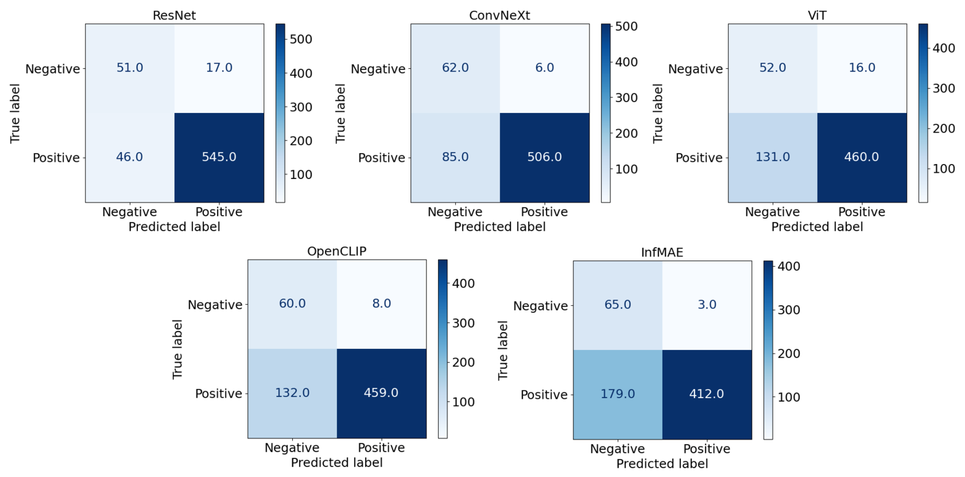
4.5. Results with MASATI Dataset

We evaluate the effectiveness of the proposed inpainting-based image augmentation method using another public dataset, MASATI [26]. As outlined in Section 2, images from two classes, “Coast” and “Coast & Ship”, are utilized for the binary classification task. Each class is randomly divided into train and test sets with an 8:2 ratio. Following [27], all images are resized to $224\times 224$. We adopt the same experimental setup used in the AP landmine experiments. We omit InfMAE in the evaluation as the model is designed to deal with infrared images. Two experiments are conducted, one with and another without the proposed inpainting-based image augmentation. To assess the model’s reliance on spurious features, we use all images from the “Sea” class along with the synthetic ship-free images (i.e., inpainted version of “Coast & Ship” test images). Inpainting masks are generated from the annotated bounding boxes provided in the MASATI dataset. Since the original bounding boxes tightly enclose the ships, we expand each bounding box by five pixels in all directions. The “Sea” and synthetic ship-free image sets contain a total of 1022 and 207 images, respectively.

Our results in

Table 7. Precision, recall, and F1-score of the positive class (“Coast & Ship”) and numbers of false positives for the “Sea” class and synthetic ship-free images.

Model	ResNet	ConvNeXt	ViT	OpenCLIP
Precision	0.976	0.986	0.986	0.956
Recall	0.961	0.986	0.990	0.937
F1-score	0.968	0.986	0.988	0.946
# of false pos.(Sea)	69	208	202	433
# of false pos.(synthetic)	113	177	187	184

and

Table 8. Precision, recall, and F1-score of the positive class (“Coast & Ship”) and numbers of false positives for the “Sea” class and synthetic ship-free images when the proposed inpainting-based augmentation is adopted.

Model	ResNet	ConvNeXt	ViT	OpenCLIP
Precision	0.989	0.980	0.984	0.927
Recall	0.908	0.947	0.884	0.792
F1-score	0.947	0.963	0.931	0.854
# of false pos.(Sea)	22	14	18	494
# of false pos.(synthetic)	16	14	39	164

highlight several important observations. First, the models trained with the proposed inpainting-based augmentation show slightly lower classification performance compared to those trained without it. However, the models without the proposed augmentation produce a large number of false positives in both the “Sea” and synthetic ship-free image sets. This indicates a strong reliance on spurious features and suggests that these models overfit to the training data. Second, the inpainting-based augmentation significantly reduces the number of false positives. This demonstrates that the proposed inpainting method is effective at mitigating the influence of spurious features and promoting the model to focus on features related to the object of interest. Third, OpenCLIP consistently underperforms compared to other models on both the AP landmine and MASATI datasets. This result suggests that OpenCLIP may be less suitable for classification tasks involving small objects.

5. Conclusions

In this work, we propose a simple deep learning-based framework for the classification of long-wave infrared AP landmine images. By carefully analyzing the limitations of the available dataset, specifically the limited number of dataset and the small spatial size of AP landmines, we incorporate techniques originally developed for broader computer vision tasks. In particular, we leverage transfer learning and attention-based multiple instance learning to address these challenges. Additionally, inspired by recent findings on the behavior of ImageNet pre-trained models, we introduce an inpainting-based image augmentation method to reduce the influence of spurious features on model predictions. Among several pre-trained models, our proposed framework achieves the best performance when using a pre-trained ConvNeXt model in combination with ABMIL. Nevertheless, a limitation of this study is the lack of variety in the image background and size of the dataset used in the experiments. We hope that this work provides valuable insights for researchers and serves as a starting point for further studies in infrared AP landmine detection.

References

1. Núñez-Nieto, X.; Solla, M.; Gómez-Pérez, P.; Lorenzo, H. GPR signal characterization for automated landmine and UXO detection based on machine learning techniques. Remote Sens. 2014, 6, 9729–9748. [Google Scholar] [CrossRef]
2. Vivoli, E.; Bertini, M.; Capineri, L. Deep learning-based real-time detection of surface landmines using optical imaging. Remote Sens. 2024, 16, 677. [Google Scholar] [CrossRef]
3. Forero-Ramírez, J.C.; García, B.; Tenorio-Tamayo, H.A.; Restrepo-Girón, A.D.; Loaiza-Correa, H.; Nope-Rodríguez, S.E.; Barandica-López, A.; Buitrago-Molina, J.T. Detection of “legbreaker” antipersonnel landmines by analysis of aerial thermographic images of the soil. Infrared Phys. Technol. 2022, 125, 104307. [Google Scholar] [CrossRef]
4. Kaya, S.; Leloglu, U.M. Buried and surface mine detection from thermal image time series. IEEE J. Sel. Top. Appl. Earth Obs. Remote Sens. 2017, 10, 4544–4552. [Google Scholar] [CrossRef]
5. Özdeğer, T.; Davidson, J.L.; Van Verre, W.; Marsh, L.A.; Lionheart, W.R.; Peyton, A.J. Measuring the magnetic polarizability tensor using an axial multi-coil geometry. IEEE Sens. J. 2021, 21, 19322–19333. [Google Scholar] [CrossRef]
6. García-Fernández, M.; López, Y.Á.; Andrés, F.L.H. Airborne multi-channel ground penetrating radar for improvised explosive devices and landmine detection. IEEE Access 2020, 8, 165927–165943. [Google Scholar] [CrossRef]
7. García-Fernández, M.; Álvarez-Narciandi, G.; López, Y.Á.; Andrés, F.L.H. Improvements in GPR-SAR imaging focusing and detection capabilities of UAV-mounted GPR systems. ISPRS J. Photogramm. Remote Sens. 2022, 189, 128–142. [Google Scholar] [CrossRef]
8. Makki, I.; Younes, R.; Francis, C.; Bianchi, T.; Zucchetti, M. A survey of landmine detection using hyperspectral imaging. ISPRS J. Photogramm. Remote Sens. 2017, 124, 40–53. [Google Scholar] [CrossRef]
9. Khodor, M.; Makki, I.; Younes, R.; Bianchi, T.; Khoder, J.; Francis, C.; Zucchetti, M. Landmine detection in hyperspectral images based on pixel intensity. Remote Sens. Appl. Soc. Environ. 2021, 21, 100468. [Google Scholar] [CrossRef]
10. Kim, J.H.; Kim, J.; Joung, J. Siamese hyperspectral target detection using synthetic training data. Electron. Lett. 2020, 56, 1116–1118. [Google Scholar] [CrossRef]
11. Baur, J.; Steinberg, G.; Nikulin, A.; Chiu, K.; de Smet, T.S. Applying deep learning to automate UAV-based detection of scatterable landmines. Remote Sens. 2020, 12, 859. [Google Scholar] [CrossRef]
12. Qiu, Z.; Guo, H.; Hu, J.; Jiang, H.; Luo, C. Joint fusion and detection via deep learning in UAV-borne multispectral sensing of scatterable landmine. Sensors 2023, 23, 5693. [Google Scholar] [CrossRef]
13. Deans, J.; Gerhard, J.; Carter, L. Analysis of a thermal imaging method for landmine detection, using infrared heating of the sand surface. Infrared Phys. Technol. 2006, 48, 202–216. [Google Scholar] [CrossRef]
14. Tenorio-Tamayo, H.A.; Forero-Ramírez, J.C.; García, B.; Loaiza-Correa, H.; Restrepo-Girón, A.D.; Nope-Rodríguez, S.E.; Barandica-López, A.; Buitrago-Molina, J.T. Dataset of thermographic images for the detection of buried landmines. Data Brief 2023, 49, 109443. [Google Scholar] [CrossRef]
15. Ren, S.; He, K.; Girshick, R.; Sun, J. Faster r-cnn: Towards real-time object detection with region proposal networks. In Advances in Neural Information Processing Systems 28; NeurIPS: San Diego, CA, USA, 2015. [Google Scholar]
16. He, K.; Zhang, X.; Ren, S.; Sun, J. Deep residual learning for image recognition. In Proceedings of the 2016 IEEE Conference on Computer Vision and Pattern Recognition, Las Vegas, NV, USA, 27–30 June 2016; pp. 770–778. [Google Scholar]
17. Solawetz, J. What is YOLOv8? A Complete Guide; Technical Report; Ultralytics: Frederick, MD, USA, 2024. [Google Scholar]
18. Kaya, S.; Leloglu, U.M.; Tumuklu Ozyer, G. Robust landmine detection from thermal image time series using Hough transform and rotationally invariant features. Int. J. Remote Sens. 2020, 41, 725–739. [Google Scholar] [CrossRef]
19. Tenorio-Tamayo, H.A.; Nope-Rodríguez, S.E.; Loaiza-Correa, H.; Restrepo-Girón, A.D. Detection of anti-personnel mines of the “leg breakers” type by analyzing thermographic images captured from a drone at different heights. Infrared Phys. Technol. 2024, 142, 105567. [Google Scholar] [CrossRef]
20. Edwards, T.; Nibouche, M.; Withey, D. Deep learning-based detection of surface and buried landmines. In Proceedings of the 2024 30th International Conference on Mechatronics and Machine Vision in Practice (M2VIP), Leeds, UK, 3–5 October 2024; IEEE: Piscataway, NJ, USA, 2024; pp. 1–6. [Google Scholar]
21. Song, H.; Kim, M.; Park, D.; Shin, Y.; Lee, J.G. Learning From Noisy Labels with Deep Neural Networks: A Survey. IEEE Trans. Neural Netw. Learn. Syst. 2023, 34, 8135–8153. [Google Scholar] [CrossRef]
22. Rezvani, S.; Wang, X. A broad review on class imbalance learning techniques. Appl. Soft Comput. 2023, 143, 110415. [Google Scholar] [CrossRef]
23. Alves, R.H.F.; de Deus Junior, G.A.; Marra, E.G.; Lemos, R.P. Automatic fault classification in photovoltaic modules using Convolutional Neural Networks. Renew. Energy 2021, 179, 502–516. [Google Scholar] [CrossRef]
24. Yao, J.; Zhu, X.; Jonnagaddala, J.; Hawkins, N.; Huang, J. Whole slide images based cancer survival prediction using attention guided deep multiple instance learning networks. Med. Image Anal. 2020, 65, 101789. [Google Scholar] [CrossRef] [PubMed]
25. Deng, J.; Dong, W.; Socher, R.; Li, L.J.; Li, K.; Fei-Fei, L. Imagenet: A large-scale hierarchical image database. In Proceedings of the 2009 IEEE Conference on Computer Vision and Pattern Recognition, Miami, FL, USA, 20–25 June 2009; pp. 248–255. [Google Scholar]
26. Alashhab, S.; Gallego, A.J.; Pertusa, A.; Gil, P. Precise ship location with cnn filter selection from optical aerial images. IEEE Access 2019, 7, 96567–96582. [Google Scholar] [CrossRef]
27. Gallego, A.J.; Pertusa, A.; Gil, P. Automatic ship classification from optical aerial images with convolutional neural networks. Remote Sens. 2018, 10, 511. [Google Scholar] [CrossRef]
28. Aldoğan, C.F.; Aksu, K.; Demirel, H. Enhancement of Sentinel-2A Images for Ship Detection via Real-ESRGAN Model. Appl. Sci. 2024, 14, 11988. [Google Scholar] [CrossRef]
29. Zuo, G.; Zhou, J.; Meng, Y.; Zhang, T.; Long, Z. Night-time vessel detection based on enhanced dense nested attention network. Remote Sens. 2024, 16, 1038. [Google Scholar] [CrossRef]
30. Oquab, M.; Darcet, T.; Moutakanni, T.; Vo, H.; Szafraniec, M.; Khalidov, V.; Fernandez, P.; Haziza, D.; Massa, F.; El-Nouby, A.; et al. Dinov2: Learning robust visual features without supervision. arXiv 2023, arXiv:2304.07193. [Google Scholar]
31. Zhang, J.; Huang, J.; Jin, S.; Lu, S. Vision-language models for vision tasks: A survey. IEEE Trans. Pattern Anal. Mach. Intell. 2024, 46, 5625–5644. [Google Scholar] [CrossRef] [PubMed]
32. Zbontar, J.; Jing, L.; Misra, I.; LeCun, Y.; Deny, S. Barlow twins: Self-supervised learning via redundancy reduction. In Proceedings of the 38th International Conference on Machine Learning, Online, 18–24 July 2021; pp. 12310–12320. [Google Scholar]
33. He, K.; Chen, X.; Xie, S.; Li, Y.; Dollár, P.; Girshick, R. Masked autoencoders are scalable vision learners. In Proceedings of the 2022 IEEE/CVF Conference on Computer Vision and Pattern Recognition, New Orleans, LA, USA, 18–24 June 2022; pp. 16000–16009. [Google Scholar]
34. Caron, M.; Touvron, H.; Misra, I.; Jégou, H.; Mairal, J.; Bojanowski, P.; Joulin, A. Emerging properties in self-supervised vision transformers. In Proceedings of the IEEE/CVF Conference on Computer Vision and Pattern Recognition (CVPR), Montreal, BC, Canada, 11–17 October 2021; pp. 9650–9660. [Google Scholar]
35. Corley, I.; Robinson, C.; Dodhia, R.; Ferres, J.M.L.; Najafirad, P. Revisiting pre-trained remote sensing model benchmarks: Resizing and normalization matters. In Proceedings of the IEEE Computer Society Conference on Computer Vision and Pattern Recognition, Seattle, WA, USA, 17–18 June 2024; pp. 3162–3172. [Google Scholar]
36. Kim, J.H.; Kwon, G.R. Efficient Classification of Photovoltaic Module Defects in Infrared Images. IEEE Signal Process. Lett. 2025, 32, 2389–2393. [Google Scholar] [CrossRef]
37. Ciga, O.; Xu, T.; Martel, A.L. Self supervised contrastive learning for digital histopathology. Mach. Learn. Appl. 2022, 7, 100198. [Google Scholar] [CrossRef]
38. Liu, Z.; Mao, H.; Wu, C.Y.; Feichtenhofer, C.; Darrell, T.; Xie, S. A convnet for the 2020s. In Proceedings of the 2022 IEEE/CVF Conference on Computer Vision and Pattern Recognition, New Orleans, LA, USA, 18–24 June 2022; pp. 11976–11986. [Google Scholar]
39. Dosovitskiy, A.; Beyer, L.; Kolesnikov, A.; Weissenborn, D.; Zhai, X.; Unterthiner, T.; Dehghani, M.; Minderer, M.; Heigold, G.; Gelly, S.; et al. An image is worth 16×16 words: Transformers for image recognition at scale. arXiv 2020, arXiv:2010.11929. [Google Scholar]
40. Radford, A.; Kim, J.W.; Hallacy, C.; Ramesh, A.; Goh, G.; Agarwal, S.; Sastry, G.; Askell, A.; Mishkin, P.; Clark, J.; et al. Learning transferable visual models from natural language supervision. In Proceedings of the 38th International Conference on Machine Learning, Virtual, 18–24 July 2021; pp. 8748–8763. [Google Scholar]
41. Liu, F.; Gao, C.; Zhang, Y.; Guo, J.; Wang, J.; Meng, D. InfMAE: A foundation model in the infrared modality. In Proceedings of the ECCV 2024: 18th European Conference, Milan, Italy, 29 September–4 October 2024; pp. 420–437. [Google Scholar]
42. Yu, W.; Zhou, P.; Yan, S.; Wang, X. Inceptionnext: When inception meets convnext. In Proceedings of the 2024 IEEE/CVF Conference on Computer Vision and Pattern Recognition, Seattle, WA, USA, 16–22 June 2024; pp. 5672–5683. [Google Scholar]
43. Sandler, M.; Howard, A.; Zhu, M.; Zhmoginov, A.; Chen, L.C. Mobilenetv2: Inverted residuals and linear bottlenecks. In Proceedings of the 2018 IEEE/CVF Conference on Computer Vision and Pattern Recognition, Salt Lake City, UT, USA, 18–23 June 2018; pp. 4510–4520. [Google Scholar]
44. Raghu, M.; Unterthiner, T.; Kornblith, S.; Zhang, C.; Dosovitskiy, A. Do vision transformers see like convolutional neural networks? Adv. Neural Inf. Process. Syst. 2021, 34, 12116–12128. [Google Scholar]
45. Cherti, M.; Beaumont, R.; Wightman, R.; Wortsman, M.; Ilharco, G.; Gordon, C.; Schuhmann, C.; Schmidt, L.; Jitsev, J. Reproducible scaling laws for contrastive language-image learning. In Proceedings of the 2023 IEEE/CVF Conference on Computer Vision and Pattern Recognition (CVPR), Vancouver, BC, Canada, 17–24 June 2023; pp. 2818–2829. [Google Scholar]
46. Ilse, M.; Tomczak, J.; Welling, M. Attention-based deep multiple instance learning. In Proceedings of the 2018 International Conference on Machine Learning and Data Engineering, Stockholm, Sweden, 10–15 July 2018; pp. 2127–2136. [Google Scholar]
47. Dauphin, Y.N.; Fan, A.; Auli, M.; Grangier, D. Language modeling with gated convolutional networks. In Proceedings of the 34th International Conference on Machine Learning, Sydney, Australian, 6–11 August 2017; pp. 933–941. [Google Scholar]
48. Moayeri, M.; Pope, P.; Balaji, Y.; Feizi, S. A comprehensive study of image classification model sensitivity to foregrounds, backgrounds, and visual attributes. In Proceedings of the 2022 IEEE/CVF Conference on Computer Vision and Pattern Recognition, New Orleans, LA, USA, 18–24 June 2022; pp. 19087–19097. [Google Scholar]
49. Kirichenko, P.; Izmailov, P.; Wilson, A.G. Last layer re-training is sufficient for robustness to spurious correlations. In Proceedings of the International Conference on Learning Representations, Kigali, Rwanda, 1–5 May 2023. [Google Scholar]
50. Fatima, M.; Jung, S.; Keuper, M. Corner Cases: How Size and Position of Objects Challenge ImageNet-Trained Models. arXiv 2025, arXiv:2505.03569. [Google Scholar]
51. Suvorov, R.; Logacheva, E.; Mashikhin, A.; Remizova, A.; Ashukha, A.; Silvestrov, A.; Kong, N.; Goka, H.; Park, K.; Lempitsky, V. Resolution-robust large mask inpainting with fourier convolutions. In Proceedings of the IEEE/CVF Winter Conference on Applications of Computer Vision (WACV), Waikoloa, HI, USA, 3–8 January 2022; pp. 2149–2159. [Google Scholar]
52. Selvaraju, R.R.; Cogswell, M.; Das, A.; Vedantam, R.; Parikh, D.; Batra, D. Grad-cam: Visual explanations from deep networks via gradient-based localization. In Proceedings of the 2017 IEEE International Conference on Computer Vision (ICCV), Venice, Italy, 22–29 October 2017; pp. 618–626. [Google Scholar]
53. Chefer, H.; Gur, S.; Wolf, L. Transformer interpretability beyond attention visualization. In Proceedings of the 2021 IEEE/CVF Conference on Computer Vision and Pattern Recognition, Montreal, BC, Canada, 11–17 October 2021; pp. 782–791. [Google Scholar]
Figure 1. Example images of areas with AP landmines (top row) and without AP landmines (bottom row). In the top row, AP landmines are buried at depths of 0, 1, 5, and 10 cm from left to right. Red boxes surrounding AP landmines are not given in the dataset and depicted here only for visualization purposes.
Applsci 15 08613 g001
Figure 2. Examples of mixed images (top row) and the corresponding cropped landmine-free regions (bottom row). An AP landmine is observed to the right of the landmine-free region in the top row.
Applsci 15 08613 g002
Figure 3. Example images of the three classes in MASATI dataset. Images of “Coast” and “Sea” classes do not contain ships while those of “Coast & Ship” do.
Applsci 15 08613 g003
Figure 4. A simple framework for extracting a single image-level feature from input images is illustrated. First, visual features are extracted using a pre-trained vision foundation model. These features are then processed through an attention-based MIL module that emphasizes discriminative features to derive a final feature appropriate for classifying AP landmine images. The top flow illustrates the process of obtaining the image-level feature for the positive class, while the bottom flow shows the corresponding process for the negative class.
Applsci 15 08613 g004
Figure 5. AP landmine images (top) and the corresponding synthetic landmine-free images (bottom) produced by the inpainting model, LaMa [51].
Applsci 15 08613 g005
Figure 6. The learning rate and loss variations in the training process.
Applsci 15 08613 g006
Figure 7. Confusion matrices when models are trained with the duplicated train set.
Applsci 15 08613 g007
Figure 8. Examples of heatmaps generated by Grad-CAM on test images for the models trained with the duplicated train set.
Applsci 15 08613 g008
Figure 9. Confusion matrices when models are trained with the inpainting-augmented train set.
Applsci 15 08613 g009
Figure 10. Examples of heatmaps generated by Grad-CAM on test images for the models trained with the inpainting-augmented train set. Red color represents higher values, while blue color represents lower values.
Applsci 15 08613 g010
Figure 11. Confusion matrices for models trained with feature maps reduced by mean pooling.
Applsci 15 08613 g011
Figure 12. Confusion matrices when foundation models combined with ABMIL are trained from scratch.
Applsci 15 08613 g012