The Use of Deep Neural Networks (DNN) in Travel Demand Modelling

Abstract

Traditional gravity models, while widely used in transport planning, often struggle to capture nonlinear spatial patterns and the heterogeneity of real-world mobility. In contrast, DNNs offer a flexible framework capable of integrating diverse explanatory variables and learning complex relationships from data. The study evaluates multiple DNN architectures trained on more than 90,000 observed OD pairs between 2477 municipalities, comparing their performance against a calibrated national gravity model. Key methodological considerations include the treatment of zero-trip observations, intra-zonal flows, and spatial aggregation levels. Results show that DNNs significantly outperform the gravity model in terms of prediction accuracy (MAE, R², GEH), with the best-performing model achieving an R² of 94%. The findings highlight the importance of data preprocessing, model architecture, and post-processing in improving predictive performance. Overall, the study demonstrates the potential of DNNs as a robust alternative to classical models in transport demand modeling, particularly when working with large, sparse, and heterogeneous datasets.

1. Introduction

This paper investigates the application of deep neural networks (DNNs) for modeling origin-destination (OD) matrices using a commuting-to-work dataset from the 2021 Polish National Census [1,2].

Understanding and modeling human mobility are fundamental components of transport planning, enabling accurate forecasting of infrastructure needs and the assessment of spatial policy impacts. For decades, the four-step travel demand model, comprising trip generation, trip distribution, mode choice and traffic assignment, has served as the backbone of transport analysis [3]. However, the increasing complexity of mobility patterns and the dynamic nature of socio-spatial changes have exposed the limitations of traditional models, particularly in capturing nonlinear relationships [4,5,6,7].

Simultaneously, the development of information technologies and the increasing availability of data from diverse sources, such as GPS systems, SIM card logins to BTS base stations, credit cards transactions, ticketing systems and IoT sensors, have opened new avenues for analyzing travel behavior [4]. In this context, artificial intelligence methods, especially deep neural networks (DNNs), are gaining prominence due to their ability to model complex, nonlinear dependencies without the need for predefined functional forms.

DNNs offer the potential to integrate diverse data sources and create flexible, scalable predictive models. They can also consolidate several classical modeling steps into a single process [4,6,7,8,9,10]. For instance, the trip generation and distribution stages could be merged into a single modeling step, thus simplifying the process and improving efficiency. Despite growing interest in the use of DNNs in transport modeling, there remains a lack of empirical studies that systematically compare their performance with classical models using real-world statistical data. This paper addresses this gap.

It should be emphasized that the primary contribution of this study is not the development of a novel neural network architecture, but rather a methodological and empirical demonstration grounded in a real-world planning context. As one of the first studies to apply DNNs to official, national-level census OD matrices in Poland, our work provides a direct comparison against a practical planning tool: the calibrated gravity model from Poland’s National Transport Model (ZMR). The goal is to show that even a simple DNN can be a robust alternative to traditional models. More importantly, this study serves as a practical guide for practitioners, providing clear recommendations on data preprocessing (e.g., handling sparse, zero-inflated datasets), model selection, and training strategies, aspects often overlooked in purely theoretical or algorithmic research.

The aim of this study is to evaluate the potential of DNNs for estimating origin-destination matrices based on publicly available data from Statistics Poland [1,2]. The analysis focuses on the first two stages of the four-step model (trip generation and trip distribution) and compares the results obtained using various DNN models with those of a calibrated gravity model. The study seeks to determine whether modern machine learning methods can effectively support transport planning in the context of data availability, especially matrix datasets.

2. Literature Review

The four-step travel demand model has long served as the foundation of transport planning, encompassing the stages of trip generation, trip distribution, mode choice, and network assignment. Despite its established role, this approach shows limitations in capturing complex, nonlinear relationships and adapting to dynamic socio-spatial and technological changes [3]. In recent decades, the use of Artificial Neural Networks (ANNs) in transport modeling, particularly for trip generation and distribution, has expanded significantly. Research trends have evolved from early experimental comparisons with classical methods to broader applications across various transport domains, including integration with big data and hybrid modeling approaches [4,5,7,11,12]. ANNs have demonstrated advantages in modeling trip distribution, especially under conditions of limited data availability. Their ability to generalize and predict missing values has made them a valuable tool in data-scarce environments [7,13,14]. A rapid increase in publications has been observed, highlighting the diversity of ANN applications in traffic forecasting, traffic control, driver behavior analysis, and autonomous vehicles. Feedforward architectures with multiple hidden layers have been most commonly used, although systematic approaches to network configuration optimization remain limited [12]. The integration of social media data, such as Twitter, into ANN and gravity models has improved model fit. ANNs have achieved higher R² values, while gravity models have shown lower RMSE values [14]. Meta-analyses [15] have shown that deep learning models such as Convolutional Neural Networks (CNNs), Long Short-Term Memory (LSTMs), Deep Belief Networks (DBNs), and Stacked Auto-Encoders (SAEs) outperform traditional machine learning algorithms like Support Vector Machines (SVMs) and Random Forests (RFs), particularly in regression and classification tasks. Hybrid models, such as CNN-LSTM, have yielded the best results due to their ability to capture spatiotemporal dependencies. Modern approaches like the Origin-Destination Convolution Recurrent Network (ODCRN), which combines convolutional and recurrent networks with semantic and dynamic context, have demonstrated superior performance in real-time mobility pattern prediction [16]. A systematic review of the literature has revealed a growing dominance of neural networks and deep learning methods since 2018, particularly in traffic management. There has also been an increase in the use of reinforcement learning and consistent application of time series analysis [9,16,17]. The importance of large datasets and further research into semi-supervised learning and hybrid techniques has been emphasized [18]. Overall, deep learning methods offer greater flexibility, scalability, and accuracy than classical approaches. Their effectiveness depends on data quality, proper training-set preparation, and appropriate model architecture and parameter selection. Models such as DNNs, CNN-LSTMs, and LSTMs are particularly useful for estimating origin-destination matrices in large urban areas with complex mobility patterns.

3. Materials and Methods

3.1. The Gravity Model

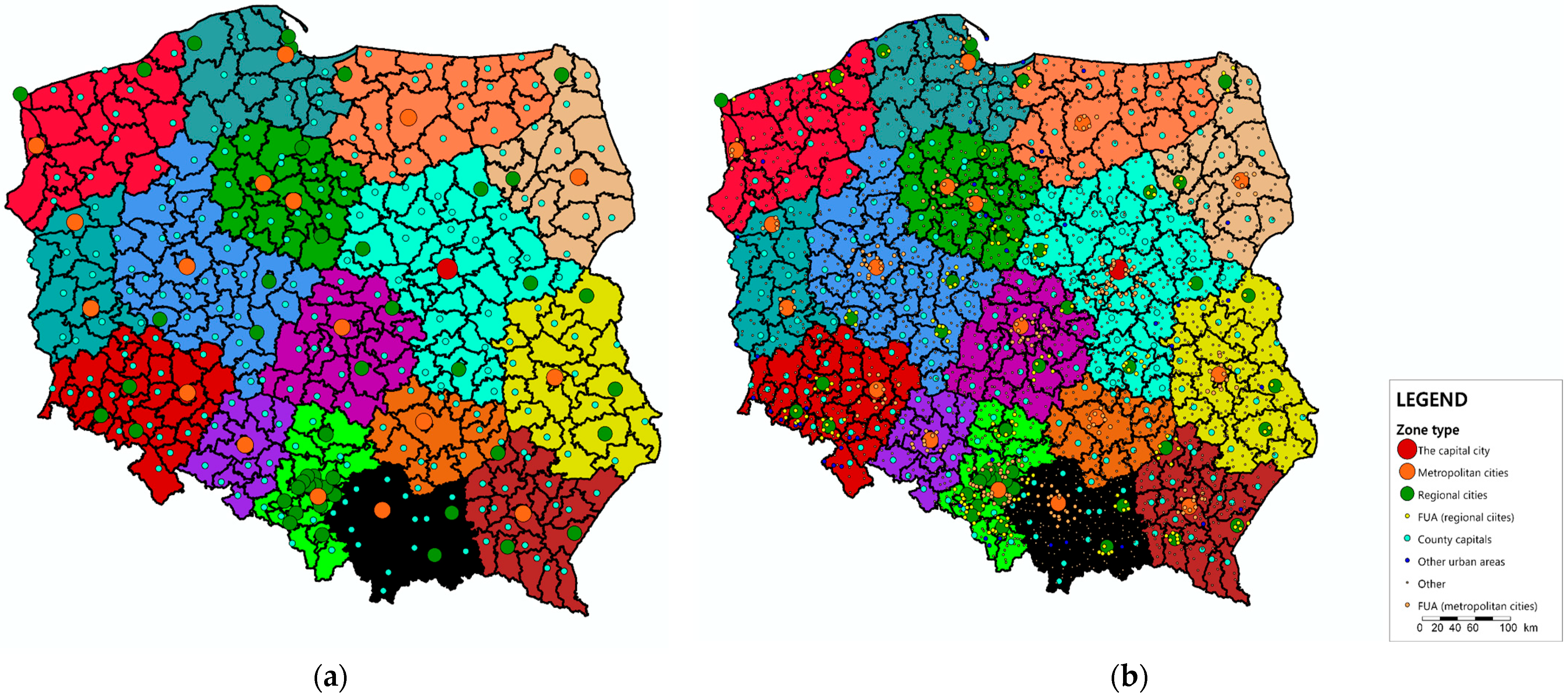
The gravity model used in this study is based on the Zintegrowany Model Ruchu (ZMR), the National Transport Model of Poland [19]. The model is based on the classical four-step methodology. In terms of the trip generation and distribution stages, it incorporates a deterrence function and trip rates defined for 13 types of municipalities (the capital city, regional capitals, county towns, and urban, rural, and mixed municipalities further differentiated by their inclusion in functional urban areas) illustrated in Figure 1a (major cities across Poland) and in Figure 1b (all municipalities).

Since the original model reflects the Average Annual Daily Traffic (AADT), the trip generation and distribution stages in this study were scaled to match the total number of employed residents and available jobs in each region. This adjustment ensures comparability of the final results with the observed commuting patterns and the outputs of trained DNN models.

3.2. Deep Neural Networks

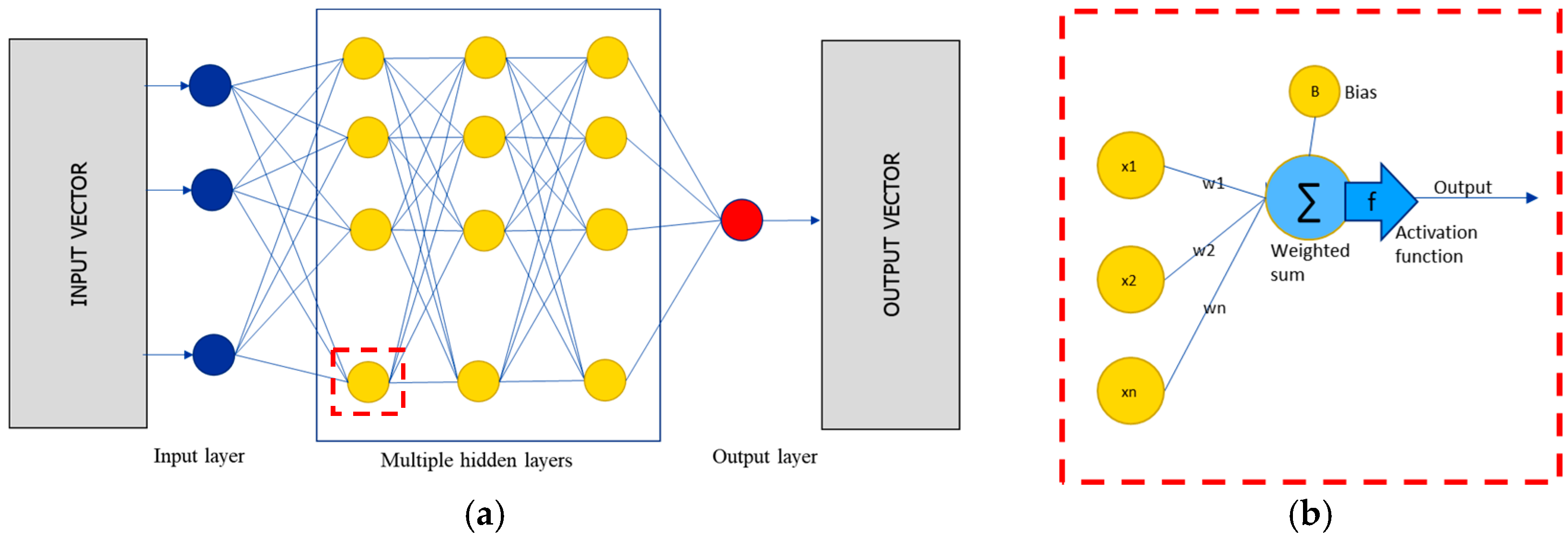
Deep Neural Networks (DNNs) are an extension of classical Artificial Neural Networks (ANNs), characterized by architectures composed of multiple hidden layers positioned between the input and output layers, as shown in Figure 2a. Each layer consists of a set of neurons that process input data using activation functions and pass the resulting signals to the next layer.

The core mechanism of a DNN is forward propagation, where input data are transformed through successive layers of the network. Each connection between neurons is associated with a weight that determines the influence of a given input on the output of the next neuron. Additionally, each neuron, as shown in Figure 2b, includes a bias parameter, which shifts the activation function and enhances the model’s flexibility in fitting complex patterns. Weights and biases are learned during the training process, which involves minimizing a loss function (e.g., Mean Absolute Error (MAE) or Mean Squared Error (MSE)) using optimization algorithms such as Adam or Stochastic Gradient Descent (SGD). During backpropagation, gradients of the loss with respect to weights and biases are computed and used to update the parameters in a direction that reduces prediction error. The use of multiple hidden layers enables DNNs to model complex, nonlinear relationships between input and output variables. In regression tasks such as estimating the number of trips between zones, the network learns to approximate a function that maps input features (e.g., population size, number of jobs, distance) to the target variable (number of trips). Nonlinear activation functions, most commonly Rectified Linear Unit (ReLU), are applied to capture nonlinearities and mitigate the vanishing gradient problem.

In this study, a sequential architecture was implemented, where data flow linearly through the network. The model consists of three hidden layers with ReLU activation functions and a single output neuron representing the predicted number of trips between a given pair of regions. The training process was based on minimizing the MAE, and the dataset was split into training, validation, and test subsets.

The decision to use a simple feedforward deep neural network (DNN) architecture was made intentionally, reflecting the characteristics of the dataset and the goals of the modeling process. The data used in this study, derived from census-based origin-destination commuting flows, are sparse, contain a high proportion of zero values, and are organized at the municipal level. These features make it particularly suitable for models that are easy to interpret, computationally efficient, and resilient to data imbalance.

3.3. Data Description

The dataset used in this study originates from the publication “Matrix of Population Flows Related to Employment—NSP 2021, Warsaw, Poznań 2024” provided by Statistics Poland. It contains information on the number of individuals commuting from municipality X to municipality Y for each pair where such a flow was observed. These values are estimates based on the 2021 National Census [1,2] and other administrative sources. Although the data do not directly represent daily or annual commuting trips, their repetitive nature allows them to be treated as a proxy for regular work-related travel patterns. This assumption enables the use of DNNs to model OD matrices. The dataset was interpreted as a Production–Attraction (PA) matrix, which better reflects the structure of commuting flows, particularly in urban areas that act as strong attractors of regional or provincial traffic. For example, Kraków (a regional capital) receives approximately 130,000 inbound commuters, while 32,000 residents commute out of the city for work. The number of individuals both living and working in Kraków is around 357,000.

The matrix data include approximately 90,000 observed commuting trips between municipality pairs. Municipalities were categorized into three types—urban, rural, and urban-rural—resulting in a total of 2477 municipalities nationwide. This yields a theoretical matrix of 2477 × 2477, or over six million OD pairs. However, the available data cover just over 1% of all possible pairs, which reflects the nature of commuting behavior: people tend to work close to where they live due to the need for frequent travel. Despite the fact that 99% of matrix cells contain zero values, these observations were retained because the absence of trips also carries meaningful information, a point further discussed in the following section. An interesting feature of the dataset is the presence of non-zero observations over unexpectedly long distances. Approximately 14% of observed non-zero flows occur over distances greater than 200 km, accounting for 1.1% of total observed commuting trips. This phenomenon is likely influenced by the data collection methodology and the growing prevalence of remote and hybrid work arrangements. Figure 3 illustrates the spatial distribution of commuting flows based on the matrix used in this study. The influence of major urban agglomerations such as the Tricity (Gdańsk–Gdynia–Sopot), Silesia, and the capital city of Warsaw is clearly visible at both regional and national scales. This pattern is partly due to the fact that the dataset is based on declared place of residence and official employer address, which may not reflect local branches or actual work locations. Additionally, many companies offering remote work are headquartered in large urban centers, particularly Warsaw and other major provincial capitals. In regional studies using similar datasets, long-distance flows (e.g., over 100 km) are often excluded to focus on daily commuting. However, travel behavior surveys [20,21] indicate that most daily commutes occur within 100 km or two hours of travel time. In this study, all observations were deliberately retained to assess the ability of models to capture nonlinear travel patterns. As shown later, the gravity model struggles to reproduce the influence of strong attractor regions over large distances, due to its inherently proportional structure.

As shown in Figure 4, the majority of journeys, constituting 93%, are confined to a distance of 100 km. An increase in the share of journeys in the 300–400 km range can be observed, which is due to the settlement pattern of Poland illustrated in Figure 5, where the main urban centers corresponding to the provincial capitals mostly fall within this distance, particularly in relation to the capital.

Table 1. Spatial distribution of trips in relation to administrative units: municipality (LAU2), county (LAU1), province (NUTS2).

Trips from Municipality X to:	Province XXX			Province YYY	Total
	County XX		County YY
	Municipality X	Municipality Y
Share of trips	69.4%	9.5%	18.1%	3.0%	100.0%
Total trips	10,371,045	1,418,022	2,707,929	454,030	14,951,026
Number of observations	4423	20,163	46,797	27,639	99,022

illustrates the spatial distribution of trips in relation to administrative units. Almost 70% of commutes occur within the municipality of residence, which can be interpreted as the matrix diagonal in this study. Around 28% of trips are made within the same province but outside the municipality of residence. Only 3% of journeys take place outside the province of residence.

3.4. Deep Neural Network Training Procedure

The training process of DNNs in this study was designed with consideration for the specific characteristics of transport data and the objective of modeling Production—Attraction matrices between administrative units. The input data included variables describing both the origin and destination zones of each trip, such as population by age group, number of jobs, and distance between regions. The target variable was the number of trips between each pair of regions. Various network configurations were tested, including different numbers of layers, neurons, and activation functions. For further analysis, a network composed of three hidden layers using the ReLU activation function was selected. A sequential architecture was adopted, consisting of three hidden layers and one output layer. The ReLU (Rectified Linear Unit) activation function was used due to its effectiveness in regression tasks and its ability to support efficient gradient propagation. The network was trained using the Adam optimization algorithm, which combines the advantages of adaptive learning rates and momentum, ensuring fast and stable convergence. The loss function was defined as Mean Absolute Error (MAE), allowing for direct interpretation of prediction errors in terms of trip counts. The dataset was split into training (80%) and test (20%) subsets, with an additional 20% of the training data used for validation during the learning process. To improve the generalization capability of one of the tested models, a regularization technique known as dropout was applied, with a dropout rate of 0.3. This method randomly deactivates a portion of neurons during training, helping to prevent overfitting. The training process was conducted across multiple model variants, differing in data scope (e.g., only inter-municipal trips, only non-zero observations, inclusion of additional explanatory variables). Each model was trained for 200 epochs with a batch size of 512. Model performance was evaluated using learning curves and MAE values for both training and test sets.

3.5. Preliminary Conclusions and Recommendations for the Main Part of the Research

During the initial phase of the study, a wide range of DNN models were tested, varying in architectural design, data aggregation levels, and internal hyperparameters. These experiments were conducted to explore the sensitivity of model performance to different configurations and to identify the most promising approaches for modeling spatial travel patterns. The results presented in this section of the paper are the outcome of dozens of experimental runs. The authors then selected representative cases that best illustrate how specific modeling choices, such as training data preparation, level of spatial granularity and neural network structure, influence the final predictive accuracy and spatial consistency of the models. This section summarizes the key insights and methodological recommendations derived from the exploratory phase of the research. These findings serve as a foundation for future work involving DNNs in transport modeling and provide practical guidance for researchers aiming to apply machine learning techniques to large-scale origin-destination data. Particular attention is given to the importance of data preprocessing, the role of spatial aggregation, and the impact of architectural complexity on model generalization and interpretability.

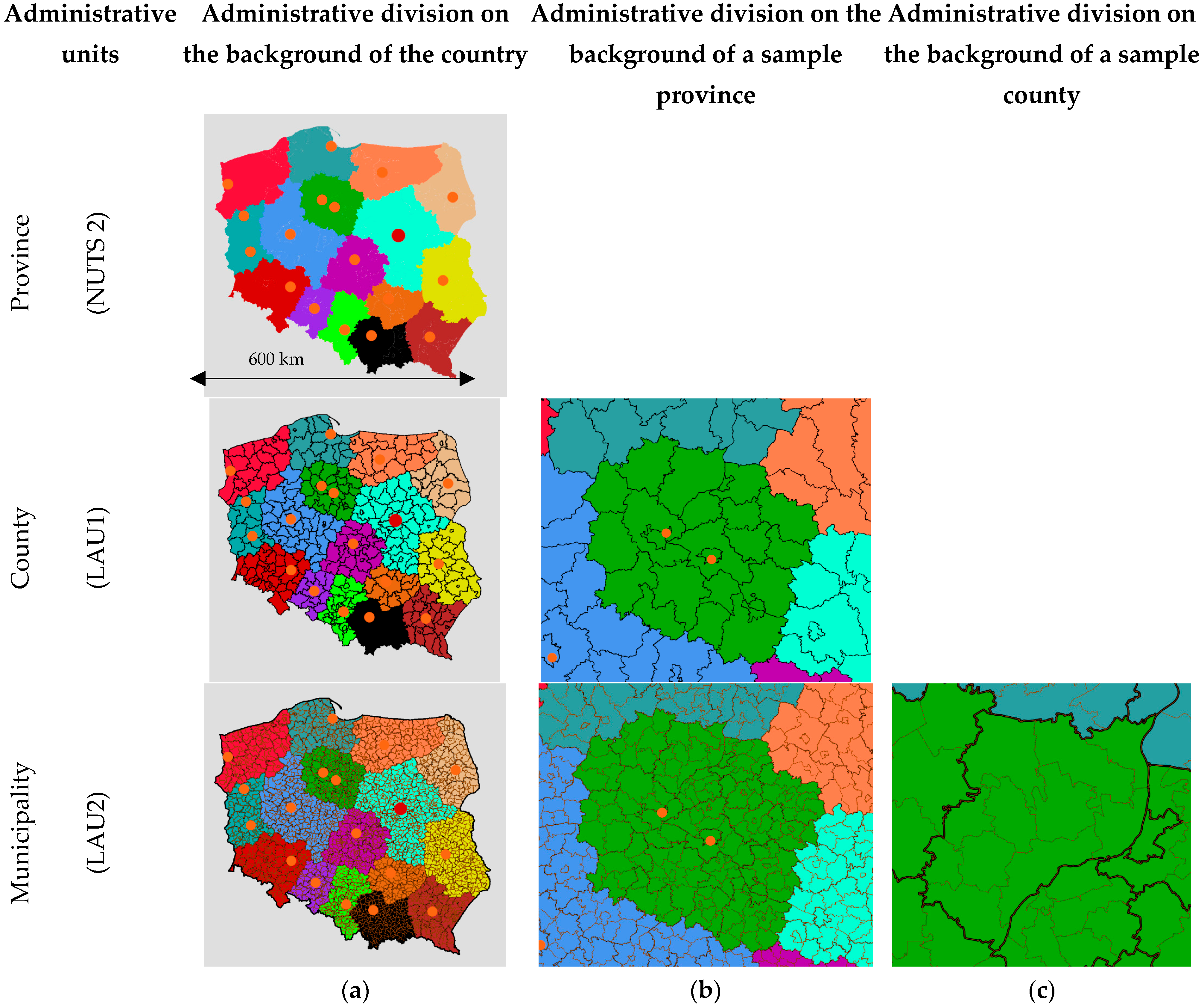
• The level of data aggregation was found to have a significant impact on model performance. The original dataset provided information at the municipal level, with urban-rural municipalities further divided into urban and rural components, resulting in a theoretical maximum of 3129 zones. For experimental purposes, the data were aggregated at three spatial levels: provinces (16), counties (380), and municipalities categorized into three types (2477). The best results were obtained using the 2477-zone municipal division. As shown in Table 2, the Root Mean Square Error (RMSE) decreased by several orders of magnitude as the spatial resolution increased, confirming that finer-grained data improve model accuracy.

Table 2. RMSE values for selected models trained at different levels of spatial aggregation.

Aggregation Level (Matrix Size)	RMSE
Provinces (NUTS1) (16 × 16)	614.20
Counties (LAU1) (380 × 380)	24.87
Municipalities (LAU2) (2477 × 2477)	0.63

Table 2. RMSE values for selected models trained at different levels of spatial aggregation.

Aggregation Level (Matrix Size)	RMSE
Provinces (NUTS1) (16 × 16)	614.20
Counties (LAU1) (380 × 380)	24.87
Municipalities (LAU2) (2477 × 2477)	0.63

• The choice of aggregation level must correspond to the availability of explanatory variables. The municipal level was selected for the final models because it provided the most comprehensive sociodemographic data, including population by age group, number of jobs, and average income levels.
• Another key finding concerns the importance of including zero-trip observations in the training data. Although most OD matrix cells contain zeros, reflecting the fact that most people work close to where they live, these zero values carry meaningful information. Excluding such observations resulted in systematic overestimation of trips, particularly for long-distance pairs that were underrepresented in the training data. Including zero-trip pairs enabled the model to learn the spatial distribution and structural characteristic of real-world commuting patterns more effectively. 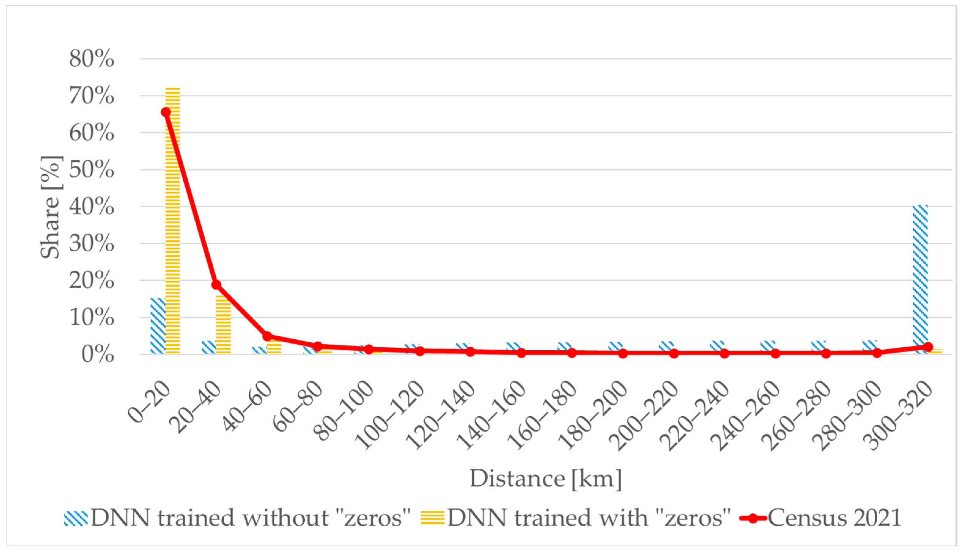Figure 6 presents a comparison of trip-length distribution histograms for trained models with and without zero values in the training dataset, based on the complete dataset. When such a model is applied to the all OD pairs, trips for distances greater than 300 km are overestimated, i.e., distances that were always non-zero in the training data. In contrast, when the vast majority of the matrix elements for distances exceeding 300 km are zero, the model more accurately estimates the number of journeys to these distances in the following sequence.

Figure 6. Trip length distribution histogram for models trained with and without zero values in the training data.

Figure 6. Trip length distribution histogram for models trained with and without zero values in the training data.

• The presence or absence of diagonal values in the OD matrix (i.e., intra-zonal trips) significantly influenced model performance for intra-zonal trips. In certain cases, excluding diagonal values during training improved the model’s ability to predict inter-zonal flows, particularly when intra-zonal values were of a substantially different magnitude compered to the remaining matrix elements. This consideration is particularly relevant when the modeling objective emphasizes regional or long-distance travel rather than local commuting. In such cases, it is essential to recognize that the results obtained on the diagonal of the matrix should not be considered when applying the trained model. It is also advisable to avoid using the model for such origin-destination pairs. However, it is worth considering the possibility of creating two separate models, one for inter-zonal trips and the other for intra-zonal trips. These models could be applied in parallel, as the matrix structure explicitly identifies which pairs correspond to diagonal elements.
• In regression-based models of travel behavior, predicted values should consistently remain non-negative, as negative trip estimates lack interpretability in real-world contexts. However, due to the mathematical properties of DNNs, it is possible for the model to generate negative outputs for certain input configurations. While applying a ReLU activation function to the final layer may appear to be a natural solution, this approach can impede backpropagation and hinder effective learning. Instead, a postprocessing procedure should be implemented, applying a ReLU function to the model outputs as an additional step to ensure all predicted values remain non-negative.
• Various network architectures were evaluated to determine the impact of depth (number of hidden layers) and neuron count on model performance. For the dataset used in this study, a minimum of three hidden layers was required to achieve satisfactory results. Increasing the number of layers improved predictive accuracy but simultaneously raised computational demands. The most effective configurations included either three layers of 64 neurons each or a tapered structure with 64, 32, and 16 neurons. Simpler architectures with fewer neurons (e.g., 16–8–4) failed to learn meaningful patterns and consistently produced zero-valued outputs.

3.6. DNN Architecture and Model Variants

The selection of an appropriate architecture for deep neural network (DNN) models is a critical and non-trivial aspect of machine learning design. Following initial exploratory experiments, the study focused on evaluating the influence of input data structure and explanatory variables on model performance, rather than extensively modifying the network architecture itself. This approach allowed for a controlled comparison of training strategies and data configurations while ensuring consistency in the underlying model design. All models shared a common architecture: a sequential feedforward neural network composed of three hidden layers for 64 neurons each (except model V3) and one output layer. The hidden layers employed the ReLU (Rectified Linear Unit) activation function, which is well-suited for regression tasks due to its simplicity and effectiveness in capturing nonlinear relationships. The output layer utilized a linear activation function to enable continuous-valued predictions. The input features included:

• Population categorized into three economic age groups (pre-working, working, and post-working age) for the origin municipality,
• Number of workplaces in the destination municipality,
• Distance in kilometeres between the origin and destination municipalities.

Training was performed using the Adam optimization algorithm, a stochastic gradient descent method based on adaptive estimation of first and second-order moments. As demonstrated by [22], Adam is computationally efficient, memory-friendly, and robust to diagonal scaling of gradients, making it suitable for problems involving large datasets and high-dimensional parameter spaces. The dataset was split into training and test sets in an 80:20 ratio, with 20% of the training data further allocated for validation. Each model was trained for 200 epochs with a batch size of 512. The loss function used was MAE, which provides a direct and interpretable measure of prediction accuracy in terms of trip counts. To examine the impact of data scope and structure, seven model variants were developed and trained:

• V1—trained exclusively on non-zero observations,
• V2—trained on the complete dataset using three hidden layers with 64 neurons each,
• V3—trained on the complete dataset using a tapered architecture with 64, 32, and 16 neurons,
• V4—trained exclusively on inter-municipal observations,
• V5—trained on all observations with an additional explanatory variable representing the average income in the destination municipality,
• V6—trained exclusively on intra-municipal observations, and
• V8—trained on the complete dataset with dropout regularization (rate = 0.3) applied during training to enhancve generalization and reduce overfitting.

These model variants were selected to demonstrate the influence of training data selection and processing, as well as architectural modifications, on predictive performance and spatial accuracy. Their comparative evaluation is presented in the following sections.

4. Results

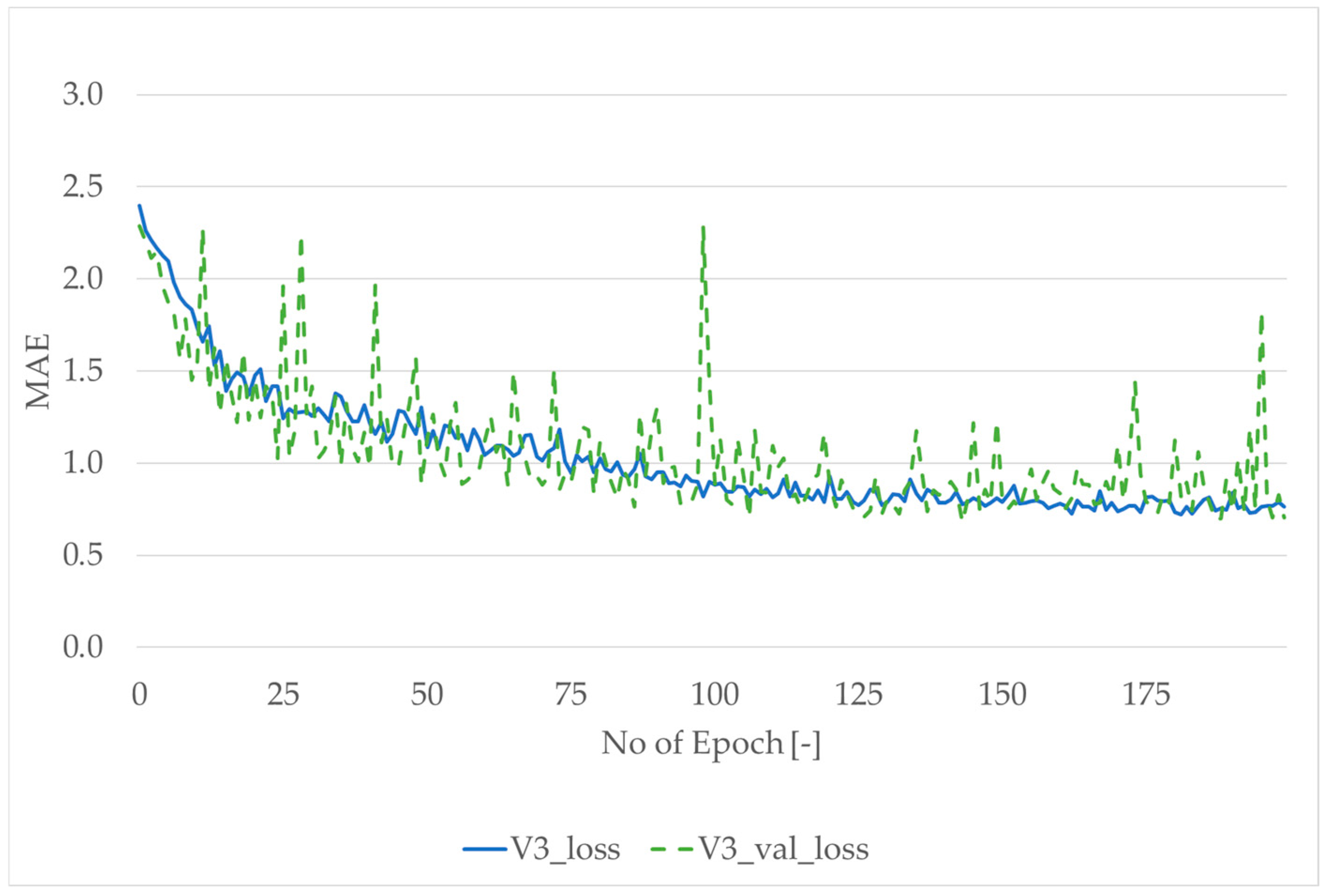
The trained DNNs were used to generate complete PA matrices based on the full set of input data. Each model produced 6,135,529 predictions, corresponding to all possible OD pairs between 2,477 municipalities (LAU2). As previously described, the dataset was split into training (80%) and test (20%) subsets, with 20% of the training data further allocated for validation during each epoch. Figure 7 presents a sample learning curve for model V3, and

Table 3. Evaluation results for trained and validation datasets.

DNN Model Name	MAE (Training Dataset)	MAE (Validation Dataset)
V1_onlyCommuters	59.46	68.45
V2_AllOD	0.95	0.94
V3_643216	0.64	0.67
V4_OnlyInterzonal	0.38	0.37
V5_Salary	0.64	0.66
V6_Intrazonal	533.06	581.03
V8_AllOD_DROPOUT	1.02	0.97

summarizes the MAE values for both training and validation datasets across all tested models.

For all models, the MAE values for the training and validation sets were closely aligned, indicating stable training and good generalization. Notably, models V1 and V6 exhibited significantly higher error values due to their limited training scope. Model V1 was trained exclusively on non-zero OD pairs, excluding the vast majority of observations (98.5%) with zero trips. This exclusion resulted in an overestimation of trips, particularly for long-distance pairs that were underrepresented in the training data. In contrast, models trained on the full dataset (including zero-trip observations) achieved significantly lower error rates. Model V4, which excluded diagonal (intra-zonal) values, delivered the best performance, suggesting that removing disproportionately large intra-zonal flows can improve inter-zonal prediction accuracy.

Beyond statistical metrics, the practical evaluation of DNN models requires assessing their ability to replicate realistic transport behavior. To this end, spatial distribution analyses were conducted, including comparisons of trip length distribution histograms and average trip lengths. These comparisons were made not only against the observed data but also relative to the gravity model. To ensure comparability with traditional transport models, additional postprocessing was applied to the DNN outputs. Specifically, some models produced negative trip values for a small number of OD pairs, which is not meaningful in real-world contexts (

Table 4. Summary of negative values across DNN models.

Model	Number of OD Pairs with Negative Values	Sum of Results for OD Pairs with Negative Values
COMMUTERS	-	-
V0_gravity	-	-
V1_onlyCommuters	-	-
V2_AllOD	29	−110
V3_643216	17	−167
V4_OnlyInterzonal	-	-
V5_Salary	1,710,202	−35,509
V6_Intrazonal	-	-
V8_AllOD_DROPOUT	-	-

). For example, model V5 generated approximately 1.7 million OD pairs with negative values, totaling 35,509 trips. This corresponds to an average of −0.02 trips per affected pair. Despite this, the model performed well during training and validation. To correct these outputs, a ReLU function (max (0, x)) was applied post hoc, ensuring that all predictions were non-negative and suitable for further analysis.

Following the application of post-processing to eliminate negative predictions in models V2, V3, and V5, a comparative analysis of spatial distribution was conducted. This included evaluating the average trip length and generating histograms of trip distances, focusing exclusively on inter-zonal trips. Among all models shown in

Table 5. Comparison of DNN models results with the base dataset and gravity model.

Model	Avg Interzonal Trip	Diff Avg	Total Trips (Interzonal OD)	Diff % Total Trips (Interzonal OD)	Total Trips (All OD)	Diff % Total Trips (All OD)
COMMUTERS	42.6	x	4,579,981	x	14,951,026	x
V0_gravity	31.8	−25%	4,638,936	1%	14,950,969	0%
V1_onlyCommuters	258.0	505%	22,267,147	386%	31,979,020	114%
V2_AllOD	37.0	−13%	4,044,406	−12%	11,930,114	−20%
V3_643216	40.0	−6%	4,055,178	−11%	14,203,123	−5%
V4_OnlyInterzonal	41.8	−2%	3,597,752	−21%	4,143,334	−72%
V5_Salary	36.6	−14%	3,865,505	−16%	14,402,262	−4%
V6_Intrazonal	405.0	850%	897,656,242,303	19,599,463%	897,666,891,303	6,003,949%
V8_AllOD_DROPOUT	32.5	−24%	2,390,852	−48%	2,390,852	−84%

Best results are highlighted in bold.

, V4 demonstrated the best alignment with observed data in terms of average trip length. This model, trained without intra-zonal observations, effectively captured the spatial structure of commuting flows. Model V8 also yielded noteworthy results. Due to the use of dropout regularization, it exhibited the highest level of generalization and produced outputs most similar to those of the gravity model. In terms of total trip volume, most DNN models underestimated the aggregate number of inter-zonal trips. Conversely, models trained on limited datasets (specifically V1 and V6) tended to overestimate total trips. These discrepancies highlight the importance of training data scope and the inclusion of zero-trip observations. The gravity model (V0) showed the smallest deviation from the observed total, but this was largely due to the use of balancing procedures. These included adjustments to row and column sums and diagonal values to match predefined totals and shares. Without these corrective steps, the discrepancies would have reached several dozen percent, underscoring the limitations of proportional models in capturing complex spatial dynamics.

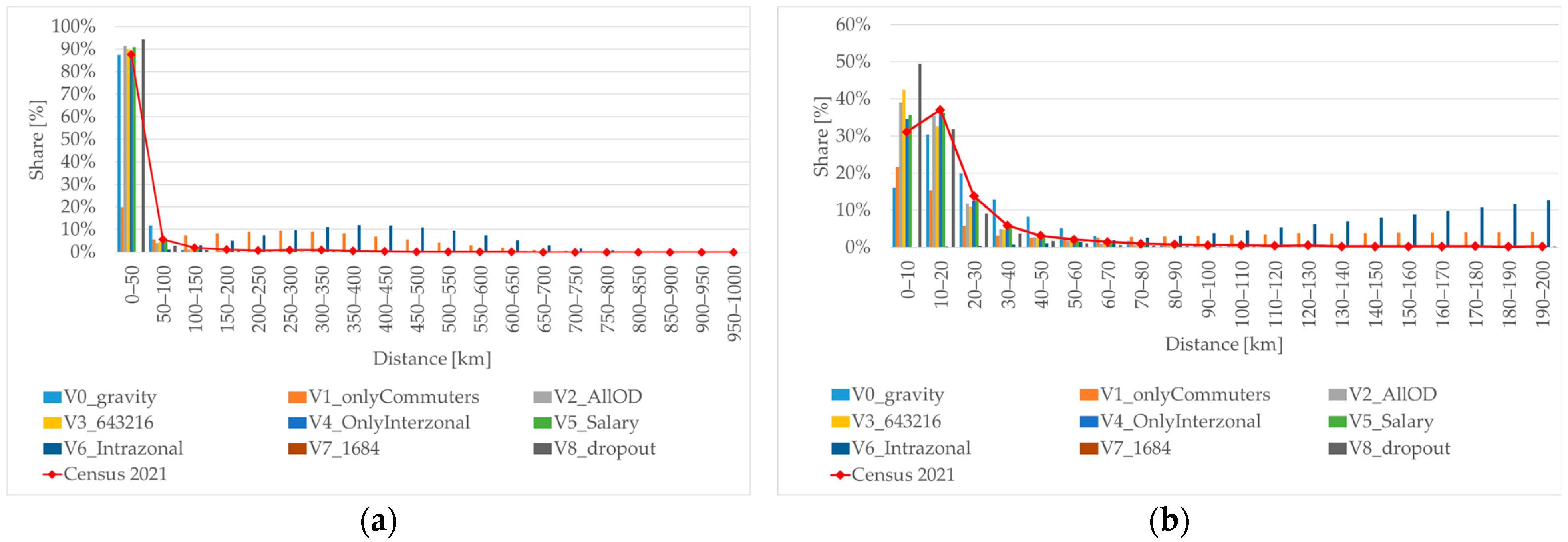
To further evaluate the spatial behavior of the models, trip length distributions were analyzed in Figure 8 using histograms for two ranges: up to 1000 km (Figure 8a) and up to 200 km (Figure 8b). These visualizations provide insight into how effectively each model captures the real-world structure of commuting flows. Model V4 demonstrated the best fit, both in terms of average trip length and distribution shape. By excluding intra-zonal trips, this model focused more effectively on inter-regional patterns, producing a realistic representation of long-distance commuting behavior. Interestingly, models trained on limited datasets, such as V1 and V6, exhibited a flattened distribution, indicating a lack of sensitivity to distance. This suggests that without zero-trip observations, the model may fail to learn the natural decay of trip frequency with increasing distance. Including zero values in the training data helps the network distinguish between plausible and implausible OD pairs, especially for longer distances.

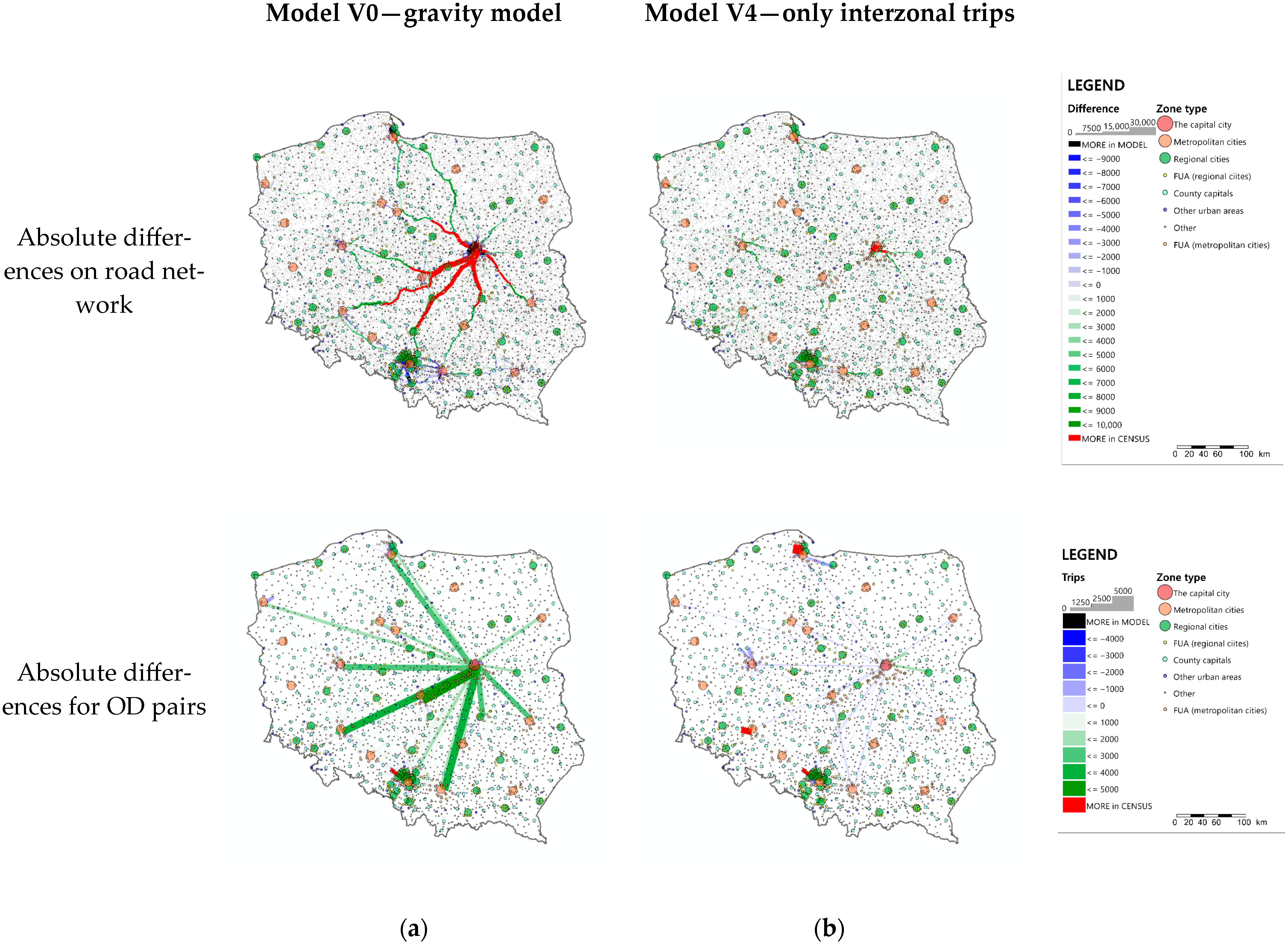
To visualize and compare the model outputs within a transport network context, a simplified traffic assignment procedure was applied using the National Transport Model for Poland. An incremental assignment method was implemented with a single iteration distributing 100% of the demand. This approach ensures that each origin-destination (OD) pair follows a consistent path, independent of network congestion or travel cost, enabling direct spatial comparison of the resulting matrices. To assess spatial differences, road segments located at county (LAU1) boundaries were selected. Figure 9 presents absolute differences in assigned traffic volumes between the base matrix and two models: the gravity model (V0) and the DNN model trained exclusively on inter-zonal data (V4). The gravity model failed to capture flows between major urban centers, which deviate from the proportional assumptions typically used in such models. These limitations are particularly evident for trips exceeding 100–150 km.

In addition to spatial analysis, a classical validation was conducted using standard transport modeling metrics: R², GEH and percentage deviation. These metrics were calculated for all selected road segments at county intersections and are summarized in

Table 6. Validation results for traffic assignment results.

Model Version	V0	V1	V2	V3	V4	V5	V6	V8
GEH: Avg	12.4	142.1	9.2	8.9	7.8	9.5	14,671.4	15.6
GEH: <20.0	85%	17%	87%	88%	90%	86%	2%	75%
Deviation: Avg	48%	88%	42%	41%	39%	43%	100%	57%
Deviation: Avg weighted	43%	83%	33%	30%	27%	35%	100%	67%
Deviation: <20%	18%	2%	22%	25%	26%	22%	0%	12%
Model/Census	0.90	30.39	0.81	0.85	0.83	0.76	279,724.14	0.37
RSQ	61%	27%	89%	91%	94%	92%	0%	72%

Best results are highlighted in bold.

.

The comparative analysis clearly indicates that model V4 (Figure 10) achieved the best overall performance across all validation metrics. Notably, the R² values for DNN models V2, V3, V4, and V5 consistently exceeded 90%, whereas the gravity model (V0) reached only 61%. Model V8, despite its generalization capabilities due to dropout regularization, produced results more comparable to the gravity model, both in terms of deviation and R²

5. Discussion

As stated in the introduction, the novelty of this study lies in its methodological and applied focus rather than algorithmic innovation. While gravity models and the four-step approach remain dominant in transport planning practice due to their simplicity and institutional acceptance, their inherent proportional structure fails to capture the heterogeneity and nonlinearity of modern mobility. Our findings demonstrate that even a standard feedforward DNN, without a novel architecture, significantly outperforms a professionally calibrated national gravity model in predictive accuracy (R² of 94% for the best DNN vs. 61% for the gravity model). This underscores a crucial point: the barrier to improving transport demand forecasting may not be the development of more complex algorithms, but rather the adoption of existing data-driven methods capable of learning from sparse and complex real-world data.

The application of DNNs to OD or PA matrix modeling represents a significant advancement in modernizing traditional transport planning methodologies. The experiments conducted in this study demonstrate that DNNs can capture complex spatial and demographic relationships that are difficult to model using classical approaches such as gravity models. This capability proved particularly valuable in the context of flows between large urban agglomerations, where nonlinear mobility patterns are prevalent and traditional proportional models fall short. One of the key insights from the study is the critical role of input data quality and structure. Models trained on complete datasets (including zero-trip observations) exhibited greater stability and better alignment with observed commuting behavior. Excluding zero values led to systematic overestimation of trips, especially for long distance OD pairs. This finding underscores the importance of treating the absence of trips as meaningful information rather than missing data. Another important aspect was the treatment of diagonal values in the OD matrix, representing intra-zonal trips. In many cases, these values were disproportionately large compared to inter-zonal flows, which distorted the learning process. Models that excluded diagonal values, such as V4, achieved better performance in predicting inter-zonal travel. This suggests that selective data filtering should be considered depending on the modeling objective.

This study also provides two key methodological implications for practice. First, the DNN approach inherently integrates the traditionally separate stages of trip generation and distribution into a single modeling step. Instead of first calculating the total number of trips produced and attracted by each zone and then allocating them, the model learns the entire relationship holistically. This integration streamlines the workflow for transport planners and reduces error propagation between sequential steps in the classical four-step model. Second, the findings emphasize the critical importance of training on sparse, zero-inflated datasets, which are characteristic of real world mobility data. Most potential OD pairs contain zero trips, and these are not missing values but essential information that defines the spatial constraints of travel. As demonstrated by the poor performance of model V1, which was trained only on non-zero flows and severely overestimated long-distance commuting, embracing the full, sparse nature of the dataset is fundamental to building models that accurately capture the structure of real-world travel patterns.

The experiments also revealed the influence of architectural complexity and regularization techniques on model performance. Deeper networks with more neurons generally delivered higher predictive accuracy but required greater computational resources. In contrast, simpler architectures failed to capture data intricacies, often resulting in underfitting or zero-valued outputs. Dropout regularization, as implemented in model V8, enhanced generalization and produced results comparable to the gravity model, although with slightly lower precision.

To clarify the modeling strategy and comparative performance, the key characteristics of each model variant are summarized below:

• Model V0 (Gravity model): Despite calibration, the gravity model struggled to capture nonlinear patterns and long-distance commuting behavior, particularly between major urban centers. This highlights the limitations of proportional assumptions in classical models.
• Model V1 (Only non-zero OD pairs): Trained exclusively on observed commuting flows, this model significantly overestimated long-distance trips due to the absence of zero-trip examples in the training data, leading to unrealistic spatial predictions.
• Model V2 (All OD pairs): Included both zero and non-zero OD pairs, producing balanced predictions and improved generalization. This model demonstrated stable performance across various spatial contexts.
• Model V3 (Tapered architecture: 64–32–16 neurons): A simplified version of V2 with reduced complexity. It achieved slightly better MAE while maintaining good spatial accuracy, making it a computationally efficient alternative.
• Model V4 (Only inter-zonal trips): Trained exclusively on inter-zonal data, this model achieved the best alignment with observed commuting patterns, particularly in long-distance flows. This suggests that excluding intra-zonal trips can improve the model’s ability to capture regional dynamics.
• Model V5 (With income variable): Incorporated average income in the destination zone as an additional feature. This model improved predictions in economically diverse regions, highlighting the value of socioeconomic variables in travel demand modeling.
• Model V6 (Only intra-zonal trips): Focused exclusively on within-municipality flows. While unsuitable for general OD modeling, it may be valuable for specialized applications targeting local mobility patterns.
• Model V8 (All OD pairs with dropout regularization): Applied dropout to enhance generalization. It produced results similar to the gravity model but with improved spatial realism, making it a strong candidate for planners seeking a balance between accuracy and simplicity.

Postprocessing of model outputs was necessary in some cases. Several models generated negative trip values, which are not interpretable in transport modeling. Applying a ReLU function to the final predictions effectively removed these anomalies and ensured the usability of the results.

Overall, the comparison between DNN-based models and the gravity model demonstrated a clear advantage for machine learning approaches in terms of predictive accuracy and spatial realism. DNNs were more effective at identifying strong regional interactions and adapt to the heterogeneity of commuting patterns, particularly in scenarios where classical models failed to account for nonlinearities and data sparsity.

The DNN models were trained on a standard laptop (Intel i7 2.3 GHz, 8 cores, 64 GB RAM) without GPU acceleration. Training time ranged from just under one hour to approximately two hours, depending on the model variant. The architecture was intentionally kept simple to ensure computational efficiency. These results demonstrate that DNN-based modeling can be implemented using widely available computing resources, making it suitable for practical planning applications. Once trained, the models can be executed quickly and applied for scenario analysis.

6. Conclusions

This study introduced a machine learning-based approach to modeling OD matrices using DNNs as an alternative to traditional gravity models. Leveraging statistical data on commuting to work flows, a series of experiments were conducted to evaluate the effects of network architecture, spatial aggregation levels, and explanatory variable selection.

The results confirm that DNNs can effectively model complex spatial and demographic dependencies, particularly in cases where classical models exhibit limitations, such as flows between major urban centers or nonlinear mobility patterns. Prediction quality was strongly influenced by the structure of the input data, with particular emphasis on including of zero-trip observations and appropriately handling intra-zonal flows.

For transport planners and policy makers, the findings of this study are directly applicable. The comparison was not merely theoretical but grounded in a real-world context, contrasting a DNN with the calibrated gravity model used in national forecasting. This approach demonstrates that DNNs are a viable tool for practical deployment. Furthermore, this paper provides actionable guidance on crucial methodological choices often overlooked in purely algorithmic studies. It highlights the importance of data preprocessing, such as including zero-trip observations and the strategic handling of intra-zonal flows. As such, this research serves as a foundational case study for applying DNNs to official census-based OD matrices in Poland, showing that these methods are not only predictively superior but also practically implementable.

Given that the models in this study were trained using standard explanatory variables (such as population, distance, and employment) commonly applied in gravity models, the transition to machine learning-based approaches can be achieved without requiring fundamentally new data sources. Trained DNNs, particularly those developed on large datasets with rich explanatory variables, can be integrated into planning workflows as a compelling alternative to classical approaches. Once trained, these models can be executed rapidly, even on standard laptops, and applied to simulate multiple planning scenarios.

Moreover, when incorporating a broader set of explanatory variables, DNNs can be further enhanced with explainable AI (xAI) techniques. Methods sush as SHAP values enable planners to better interpret the relationships learned by the model and identify the factors most influencing travel behavior. This advancement paves the way for more transparent and interpretable applications of machine learning in transport planning, bridging the gap between predictive performance and policy relevance.

Despite their black-box nature, DNNs can reproduce travel patterns and relationships that classical models often fail to capture, making them a powerful addition to the transport modeling toolkit.