Article

Reconstruction of Building LIDAR Point Cloud Based on Geometric Primitive Constrained Optimization

1
Merchant Marine College, Shanghai Maritime University, Shanghai 201306, China
2
College of Transport & Communications, Shanghai Maritime University, Shanghai 201306, China
3
College of Engineering Science and Technology, Shanghai Ocean University, Shanghai 201306, China
*
Author to whom correspondence should be addressed.
Appl. Sci. 2025, 15(20), 11286; https://doi.org/10.3390/app152011286
Submission received: 9 September 2025 / Revised: 19 October 2025 / Accepted: 20 October 2025 / Published: 21 October 2025

Abstract

This study proposes a 3D reconstruction method for LIDAR building point clouds using geometric primitive constrained optimization. It addresses challenges such as low accuracy, high complexity, and slow modeling. This new algorithm studies the reconstruction of point clouds at the level of geometric primitives and is an incremental joint optimization method based on the GPU rendering pipeline. Firstly, the building point cloud collected by the LIDAR laser scanner was preprocessed, and an initial building mesh model was constructed by the fast triangulation method. Secondly, based on the geometric characteristics of the building, geometric primitive constrained optimization rules were generated to optimize the initial mesh model (regular surface optimization, basis spline surface optimization, junction area optimization, etc.). And a view-dependent parallel algorithm was designed to optimize the calculation. Finally, the effectiveness of this approach was validated by comparing and analyzing the experimental results of different buildings’ point cloud data. This algorithm does not require data training and is suitable for outdoor surveying and mapping engineering operations. It has good controllability and adaptability, and the entire pipeline is interpretable. The obtained results can be used for serious applications, such as Building Information Modeling (BIM), Computer-Aided Design (CAD), etc.

1. Introduction

Human vision perceives the world in three dimensions. To better characterize buildings and enhance spatial cognition, it is essential to acquire both structural and appearance information. Typically, a 3D geometric representation of the building is first reconstructed, followed by texture mapping onto the mesh model. Realistic 3D building models overcome the limitations of visual perception associated with 2D representations. In recent years, advancements in LIDAR technology have made it easier to acquire large-scale building point cloud data [1]. The Oxford Radar RobotCar Dataset contains over 240,000 scans from a Navtech CTS350-X radar and 2.4 million scans from two Velodyne HDL-32E 3D LIDAR sensors [2]. This dataset provides a strong foundation for research on building point cloud reconstruction. A 3D point cloud reconstruction of building models has become a prominent research focus. It is a key technology across various research and application domains, including digital cities, urban planning, historical architecture analysis, and disaster monitoring. Despite significant efforts in building point cloud reconstruction, many challenges remain, particularly regarding reconstruction accuracy [3,4].
Although deep learning is a current research hotspot, high-stakes application scenarios, such as BIM and CAD, demand explicit semantics and interpretable editing, rather than the black-box nature and unpredictable failure cases associated with deep learning [5,6]. Furthermore, to adapt to dynamic scenes, deep learning models require frequent retraining, which limits their flexibility [7]. In our view, interpretable methods with precise control are more suitable for mission-critical applications [8]. Deep learning, as an optimization solver, has shown broad applicability across various domains.
Point cloud data can accurately represent building surface geometry. However, point clouds are often noisy and sensitive to processing techniques, which significantly impacts the robustness of building reconstruction pipelines. In this work, we adopt a “geometry-then-optimization” approach. The 3D building model is constructed through the extraction, classification, and optimization of geometric primitives. The target building point cloud is extracted from the raw LIDAR data collected in the field. A geometric model is first constructed from the point cloud, followed by optimization constrained by geometric primitives. To improve computational efficiency, we design a view-dependent incremental joint optimization strategy and leverage GPU parallelism. Geometric primitive constraints are primarily used to refine the mesh structure of building facades and junctions. After optimization, the model more closely resembles the real building geometry, with artificial surface irregularities eliminated. This method enables rapid reconstruction of large-scale, noisy building point clouds. The model supports multi-level optimization to meet varying accuracy requirements. The remainder of this paper is organized as follows: Section 2 reviews related work on building point cloud reconstruction. Section 3 details the proposed method, including data preprocessing, initial model construction, and the optimization strategy. Section 4 presents experimental validation and a comparative analysis. Finally, Section 5 concludes the paper and outlines future research directions.
The main contributions of this work are summarized as follows:
  • A reconstruction method for the building LIDAR point cloud based on geometric primitive constrained optimization is proposed, which takes into account both the reconstruction accuracy and the complex and time-consuming modeling process;
  • A geometric primitive generation method for the building LIDAR point cloud is designed for the constraint optimization;
  • A geometric primitive-based calculation method of the optimal energy equation is designed for the reconstruction method;
  • A view-dependent incremental joint optimization strategy is designed to improve the calculation efficiency.

2. Related Work

  LIDAR systems represent a cutting edge-technology in modern environmental sensing, providing high-precision 3D data of object surfaces. Recent advancements in LIDAR hardware and software (e.g., CloudCompare) have significantly improved data acquisition accuracy and speed, making it well-suited for large-scale 3D building point cloud collection due to its efficiency, short processing cycle, high accuracy, and cost-effectiveness [9]. These systems generate discrete point clouds that capture surface structures, enabling geometric feature extraction for 3D reconstruction, particularly in building-related applications [10,11].

2.1. Common Methods for 3D Reconstruction of Objects/Scenes

The common methods for 3D reconstruction of objects/scenes can be mainly divided into four categories: structure-aware reconstruction [12,13,14], semantic-aware reconstruction [15,16], the Level of Detail (LOD) approach [17], and the data-driven approach [18,19,20,21,22,23]. structure-aware reconstruction method first extracts geometry elements and relations and then performs the calculations of geometry element assembly and optimization. The geometry elements are usually lines and planes. This kind of method avoids over-regularizing of non-dominant directions. However, how to automatically detect preferred relations needs to be further studied [24]. The semantic-aware reconstruction method segments the point cloud into a set of regions with semantic labels, adopts semantic knowledge to rebuild each region or object, and finally composes a complete scene. However, the reconstruction accuracy needs to be improved. The LOD approach is mainly divided into three processes: classification, abstraction, and reconstruction. This kind of method usually uses a fixed set of LODs to describe objects/scenes. The data-driven approach is usually divided into three steps: partial reconstruction, structure analysis, and database association based on structure/context information. It is facilitated by low-quality raw data and a high-quality database model. For the current state-of-the-art data-driven approach, geometry information of objects and the relationships between them are jointly learned and embedded in the learning model by an encoder. The encoder organizes the geometry and structure features, while the decoder disentangles the features and reconstructs the 3D geometry of the object.

2.2. Methods for Building a Point Cloud

Generally, the building point cloud data can be divided into two types: those acquired by ground-based devices (terrestrial LIDAR) and those captured from the aerial LIDAR [25]. The methods for 3D reconstruction of buildings based on point cloud data absorb the basic ideas of the common 3D reconstruction methods. They can be divided into two main types: the interactive modeling method and the automatic modeling method.
Interactive reconstruction methods focus on denoising and completing incomplete data through user interaction, offering high model quality but low efficiency. Ref. [26] proposed a pipeline to consolidate imperfect scans using user-guided facade elements. Ref. [27] developed SmartBoxes using simple geometric primitives to reconstruct incomplete building data with user input. Ref. [28] combined 2D images with point clouds via bidirectional information transfer, with user markup for initialization. Ref. [29] introduced a sketch-based interactive system using optimization in adaptive 2D modeling spaces. Ref. [14] proposed PolyFit, which generates face candidates and selects an optimal subset for reconstruction.
Automatic reconstruction methods improve efficiency through structural priors or learning-based segmentation. Ref. [30] preserved structural features by reconstructing from detected primitives. Ref. [31] segmented point clouds semantically and reconstructed each part accordingly. Ref. [32] formulated Manhattan-world reconstruction as a labeling problem with aligned boxes. Ref. [33] used a rectified linear unit neural network for airborne LIDAR segmentation and model reconstruction. Ref. [34] employed a triangulated irregular network (TIN) model to extract planar regions, optimize roof faces, and generate complete models. Ref. [35] applied fuzzy c-means clustering and region growing for rooftop segmentation and wall generation. For performance improvement, ref. [36] introduced a GPU-accelerated reconstruction algorithm.
Algorithm design must consider architectural style, input type, and application [37]. Manhattan building reconstruction algorithms mostly rely on orthogonality and rectilinearity rules. Ref. [38] compared mesh-based constrained reconstruction and geometry-based modeling, concluding that the former offers higher accuracy and detail, despite greater storage cost. This study adopts a “geometry-then-optimization” strategy. As demands for reconstruction quality rise in BIM, GIS, and CAD, mesh optimization becomes increasingly critical.

3. Method

Our reconstruction approach employs a view-dependent incremental joint optimization framework, incorporating geometric primitive constraints and leveraging the GPU rendering pipeline. Geometry optimization is treated as an iterative, step-by-step process. Reconstruction is driven by changes in the 3D viewpoint, iteratively optimizing non-occluded regions within the current field of view. The optimization process is controllable, with its degree determined by accuracy requirements and the amount of calculation. Given the large volume of LIDAR point cloud data, we first perform preprocessing to extract the relevant subsets for reconstruction; we then apply a fast area expansion mesh reconstruction technique (specifically, the greedy projection triangulation algorithm [39]) to generate an initial mesh model. Finally, geometric primitive constraints are introduced to refine the mesh structure of the building model, and parallel computing is employed to accelerate the optimization. The overall algorithmic workflow is illustrated in Figure 1.

3.1. Initial Model Reconstruction

3.1.1. Data Preprocessing

Point Cloud Segmentation. The acquired point cloud data of a building scene typically contains not only the target building but also unrelated elements such as trees, pedestrians, and vehicles. To minimize the influence of irrelevant point clouds during reconstruction, the target building point cloud must be segmented from the scene. Extensive research has been conducted on point cloud segmentation, and numerous methods have been proposed [40,41]. To more accurately extract the target building point cloud, we incorporate thematic information, such as map data, building contours from remote sensing imagery, and BIM data, to guide segmentation. Specifically, segmentation is guided by the building’s base contours and height attributes derived from thematic sources.
LIDAR Point Cloud Simplification. Building models typically exhibit regularly distributed feature points, but the presence of noise can adversely affect the extraction computation. We also need to downsample the point cloud to reduce the amount of computation. Pre-filtering the raw data is essential; otherwise, reconstruction may become time-consuming and error-prone due to noise and outliers, resulting in a poorly constrained building facet. Based on the LIDAR system’s measurement parameters, the scanned point clouds are registered and merged to produce a complete dataset representing the building scene. Filters should be selected based on the characteristics of the building point cloud to perform denoising and outlier removal. We experimentally analyze the characteristics of different filtering techniques.
To filter the initial dense point cloud, we first apply a voxel filter for downsampling. This method divides the three-dimensional space into a uniform grid of cubes (voxels), replacing the coordinates of all points within each voxel with a representative point to achieve data compression. For point cloud filtering tasks such as urban models or large terrains, the voxel size parameter for each voxel is typically set to a value between 0.1 and 0.5. The representative point is typically calculated using the geometric center (center of mass) of all points within the voxel, which can be defined as Equation (1).
P v o x e l = 1 n i = 1 n P i
where P v o x e l is the coordinate of the representative point, n is the number of points contained in the voxel, and P i is the coordinate of the i-th point in the voxel. Voxel filtering can effectively compress large-scale point cloud data while preserving the model’s shape characteristics at a macro level. During the feature extraction stage, the voxel size parameter is crucial: too large a size results in loss of detail, while too small a size results in poor compression. The right size can significantly improve algorithm efficiency.
Then, the statistical filter and radius filter are selected to filter the point cloud. Statistical filters filter based on the local neighborhood distance distribution of the point cloud. For each point P i in the point cloud, the average distance d i to all k nearest neighbors is calculated. The average distance μ and standard deviation σ for the entire point cloud are then calculated to form a dynamic threshold, the core discriminant of which can be defined as Equation (2).
d i μ > α · σ
where α is the standard deviation multiplier, typically set between 1.0 and 3.0. Any point that satisfies Equation (2) is considered an outlier and removed. This method is suitable for removing sparse noise points that deviate significantly from the main point cluster due to measurement errors. Radius filters filter based on the local density of points. For each point P i , the number of its neighboring points N i within a fixed search radius r is counted. If the number of neighbors of a point falls below a set minimum value N m i n , the point is considered an outlier and removed. The criteria for this are defined as Equation (3).
N i < N m i n
Radius filtering is usually more direct and efficient than statistical filtering in removing sparsely distributed outliers, but its effect is more sensitive to the parameter settings of the search radius r and N m i n . In our experiments, the number of neighbors k of the statistical filter is set to 50; the threshold of the number of neighbors of the radius filter N m i n is set to 5, and the search radius r is set by the average nearest neighbor distance ρ of the point cloud. Usually, the value of r is set to 2 ρ .
Experimental results indicate that voxel filtering effectively simplifies point cloud data through downsampling. Details of the experimental results are presented in Section 4. The voxel filter applies a voxel grid approach to perform downsampling. It preserves the original geometric structure and features during simplification. The simplified point cloud still accurately represents the surface of the target object. The statistical filter is suitable for removing prominent outliers caused by measurement errors. The radius filter removes outliers more efficiently than the statistical filter but is more sensitive to parameter settings.

3.1.2. Mesh Reconstruction of Point Cloud Data

In this work, we construct a triangular mesh model from the pre-processed point cloud data. The resulting mesh serves as a standard format for modern rendering pipelines and facilitates spatial geometry analysis and querying.
The greedy projection triangulation algorithm [39] enables rapid reconstruction of triangular meshes from point cloud data. It is based on planar region triangulation. Starting from sample triangles selected via the Delaunay-based area expansion, the surface boundary is iteratively extended to form a complete mesh. The topological connections between 3D points are then established based on the connectivity of their 2D projections. The resulting triangular mesh constitutes the reconstructed surface model. This algorithm efficiently triangulates scattered point clouds and supports data acquired from multiple scanners with multiple connections. Poisson surface reconstruction often introduces redundant boundaries and artifacts, complicating post-processing. In this work, we adopt the greedy projection triangulation algorithm to reconstruct the pre-processed point cloud and generate the initial mesh model. For specific parameter settings, please refer to [42].

3.2. Model Optimization

The mesh model is optimized using geometric primitive constraints. We first generate geometric primitives from the point cloud. We then formulate an energy function constrained by geometric primitives to guide mesh optimization. Finally, a view-dependent parallel algorithm is developed to enhance computational efficiency.

3.2.1. Geometric Primitive Generation

Following point cloud preprocessing, we first apply the supervoxel method [43] for initial segmentation. This method better preserves object boundaries and fine structures. However, due to the discrete nature of point clouds and the presence of noise, segmentation algorithms are often sensitive to parameter settings, resulting in suboptimal outcomes. To obtain complete geometric primitives, we merge segmented regions while preserving boundary integrity. By merging adjacent patches belonging to the same primitive, we construct more complete geometric units for constrained optimization. Global geometric features alone are insufficient to determine whether two patches should be merged. We thus design a patch-merging method based on local geometric features (Figure 2). Patch merging is guided by the continuity of local geometric features. Similarly, due to signal discreteness and noise, global statistics are insufficient to classify point cloud patches into geometric primitives. We propose a spatial sparsity-based patch classification method to determine primitive categories (Figure 3). The judgment is performed via statistical analysis of local features after spatial subdivision.
To overcome the influence of the discrete nature of the point cloud and the noise, we use the K nearest feature to judge the patch junction during the patch merging calculation, which can be expressed as Equation (4).
m e r g f l a g = b o o l ( c o u n t ( i K 1 D ( p A , p i ) < D T ) c o u n t ( i K 1 D ( p A , p i ) < D T ) K 1 K 1 > 0.8 ) b o o l ( c o u n t ( j K 2 D ( p B , p j ) < D T ) c o u n t ( j K 2 D ( p B , p j ) < D T ) K 2 K 2 > 0.8 ) ,
where K 1 and K 2 are the number of other patch points around p A and p B , respectively; D T is the threshold of the distance; and D ( . ) is the distance function. The function bool is a Boolean operator used to determine whether a condition is satisfied. It returns 1 if x > 0.8 (i.e., the condition meets the threshold requirement) and 0 otherwise. The variable count denotes the number of points among the K 1 nearest neighbors P i of patch A whose distance to the reference point P A is either below or above the distance threshold D T . To determine the optimal value for K, we conduct 200 experiments. The best patch junction judgment effect is obtained when K = 0.8 .
To improve computational efficiency during patch merging, we introduce an optimization strategy. When traversing the nearest neighbors of a point, if previously visited neighbors are detected, redundant computations are skipped.

3.2.2. Construction of the Optimal Energy Equation

The joint optimization process consists of two main steps. First, thematic information is aligned with the point cloud data. The thematic information refers to auxiliary geospatial data, such as building footprint maps and roof contours derived from remote sensing imagery, which are spatially aligned with the LIDAR point cloud and serve as prior geometric constraints during reconstruction. Second, geometric primitive constraints are applied to optimize the mesh model. The overall reconstruction algorithm is outlined in Figure 4.
The algorithm begins by applying scale transformation and pose adjustment algorithms [44] to align the point cloud data with thematic information. Based on this alignment, thematic information is used to jointly infer the geometric primitive type for reconstruction.
The optimization process consists of two components: fitness error optimization of geometric primitive and junction error optimization. The first component, f i t n e s s _ e r r o r , is a function of the primitive fitting function and the original mesh geometry; the second component, j u n c t i o n _ e r r o r , captures spatial relationships between primitives in the original mesh. The overall optimization energy function is defined in Equation (5).
E r r o r = α f i t n e s s _ e r r o r + β j u n c t i o n _ e r r o r ,
where α and β are adjustable weight coefficients. fitness_error denotes the fitting error of geometric primitives, reflecting local consistency. junction_error measures continuity at primitive junctions. The weights α and β are manually tuned: α is increased to prioritize surface fitting, while β is increased to emphasize junction continuity.

3.2.3. Optimization Calculation

After constructing the initial model, we proceed to optimize it for improved representation of the building structure. Based on the generated geometric primitives and the alignment between the point cloud and thematic information, we perform optimization on the initial triangular mesh. Based on the characteristics of the building model, two types of optimization are required: surface optimization and junction area optimization. Surface optimization is further divided into regular and B-spline-based approaches. Both approaches are applicable to optimizing mesh models in large-scale building scenes. Finally, a view-dependent parallel algorithm is developed to accelerate the optimization process.
Surface Optimization. The building surface is usually relatively flat. However, due to random noise in the point cloud data, the reconstructed mesh surfaces often exhibit unevenness, which degrades both fidelity and visual quality. To address this, we construct an optimization transformation M between the mesh and the primitive constraints. The detailed computation steps are as follows:
First, regular surface optimization defines constraint surfaces for each planar region in the initial mesh. These are referred to as constraint surfaces. A plane or B-spline surface equation is constructed from the selected point cloud samples.
Second, a constraint function (Equation (6)) is defined based on the distance between the mesh and the constraint surface. The optimal transformation M is obtained by minimizing the corresponding energy cost function.
arg min M x i I M · x i S k k 2 ,
where M · x i denotes the homogeneous transformation of point x i R 3 using the 4 × 4 matrix M = R t 0 1 , with R R 3 × 3 as the rotation matrix and t R 3 as the translation vector. The set I contains all vertex coordinates in the mesh. The parameter k represents the summation over all visible geometric primitives indexed by k, and the norm · k 2 denotes a weighted 2 norm that accumulates contributions from each primitive, typically in the form k w k · 2 2 , where w k is the weight of the k-th region. The constraint term S k encodes the geometric property defined by the k-th primitive (e.g., planarity, parallelism) and serves as a target that the transformed point M · x i should adhere to. The objective function thus minimizes the weighted deviation of transformed vertices from these geometric constraints, ensuring structural consistency with predefined architectural rules.
Third, minimization of the energy cost function leads to a high-dimensional nonlinear least squares problem. The transformation M involves a large number of parameters. To improve computational efficiency, we adopt a block-wise optimization strategy. Specifically, triangles are first clustered based on their normal vectors. For each cluster, a shared local transformation matrix is estimated. This significantly reduces the number of parameters in M. A sliding clustering approach is adopted, and cosine similarity is used to measure the similarity between normal vectors. The corresponding similarity metric is defined as follows:
( a , b ) a b < ε ,
where a and b are surface normal vectors associated with adjacent points or regions, representing the local orientation of the geometry. ε is a user-defined threshold controlling the angular similarity. This condition determines whether two points or regions belong to the same cluster: if violated, a new cluster is initialized, corresponding to a separate transformation block in M. Within each cluster, the local transformation matrix is estimated using the principle of least squares. To enhance robustness, multiple points are sampled within each cluster to compute the optimal local transformation.
Finally, triangle patches corresponding to thematic constraints are projected onto the constraint surface. This completes the surface optimization process. As a result, the reconstructed surface better approximates the real building surface.
Junction Area Optimization. Similar to surface optimization, a transformation is required to refine the original mesh in the junction areas. Based on the geometric characteristics of junctions, we introduce two types of constraints: linear junction constraints and surface junction constraints. The optimization involves two cost terms: the distance between the mesh and the constraints and the subdivision cost. These two costs are interdependent. A higher subdivision cost increases the complexity of distance optimization, while larger distance deviations necessitate finer subdivision. The cost function is formulated as follows:
arg min M x i I M · x i S k k 2 + N d i v ( c ) ,
where N div ( c ) denotes the number of triangular subdivisions as a function of the local curvature c. More specifically, for each vertex x i , we define the following equation:
c ( x i ) = κ 1 ( x i ) + κ 2 ( x i ) 2 ,
where κ 1 and κ 2 are the principal curvatures of the mesh at x i , so that c measures the mean bending of the surface. Thus N div ( c ) remains constant for near-flat (linear) junctions, where we apply fixed subdivision rules, and grows with c in highly curved (surface) junctions, where optimal subdivision and transformation are determined via joint least-squares optimization.
(1)
Optimization of Linear Junction Areas
For junctions exhibiting regular linear features, the optimization leverages line constraints derived from the intersection of two planar surfaces. The local triangular mesh is refined via subdivision and spatial transformation to better conform to the actual building geometry. The procedure is as follows:
First, the intersection line of the two constraint surfaces is computed, and nearby triangle patches in the mesh are identified and marked.
Second, by fixing the subdivision cost term N div ( c ) in Equation (8), the alignment cost is minimized to solve for the initial transformation.
M 1 = arg min M x i I M · x i S k k 2 ,
where M 1 aligns the marked triangle patches with the first constraint surface. The transformed patches are then subdivided along the regular line defined by the two intersecting constraint surfaces.
Finally, we set N div ( c ) = 0 and solve a similar minimization problem to obtain a second transformation:
M 2 = arg min M x i I M · x i S k k 2 ,
where I is the set of vertices in the subdivided patch not aligned by M 1 , and S k is the second surface constraint. M 2 aligns this region to the second surface, completing the optimization of the linear junction area.
In general, each transformation step in the optimization pipeline can be denoted as M i , representing a local rigid transformation minimizing the alignment cost under specific geometric constraints.
(2)
Optimization of surface junction area
For junction areas with regular surface features, optimization is guided by a fitted constraint surface. The triangular mesh in the junction area is refined to better match the true building surface geometry. An iterative method is proposed to jointly minimize the curvature difference and subdivision cost until the vertex curvature difference meets a predefined threshold. The algorithm proceeds as follows:
First, a surface equation is fitted to represent the geometry of the junction area, which serves as the constraint surface.
Second, the distance cost is minimized to solve for the transformation M 1 . After applying the transformation, the vertex curvature is compared with that of the constraint surface. If the curvature difference is below the threshold, no subdivision is applied; otherwise, subdivision is performed. Subdivision intensity is determined by the magnitude of the curvature difference. Larger differences require multiple subdivisions, while smaller differences call for limited refinement to control the N div ( c ) cost.
A discretized fixed template is used to approximate the local optimum of the cost function. When the curvature difference exceeds ten times the threshold, three subdivisions are applied; otherwise, one is used. In each subdivision step, the midpoints of the triangle edges are added as new vertices, dividing the patch into four sub-triangles.
Third, the second step is repeated. The iteration continues until the curvature difference falls below the threshold. In the implementation, GPU shaders are used to perform computations. The shaders enable hardware-parallelized triangle subdivision, significantly improving computational efficiency.
View-Dependent Parallel Algorithm. Although previous point cloud simplification reduces computational load, the overall optimization process still requires further acceleration. We construct a hierarchical tree structure from the point cloud data to support efficient processing. This structure accelerates spatial partitioning, downsampling, and search operations. In our algorithm, the core computational tasks involve triangle patch intersection and transformation. These operations are inherently parallelizable. We design a view-dependent parallel algorithm (Figure 5) to optimize the calculation. The reconstruction process is driven by changes in the 3D viewpoint and iteratively updates non-occluded regions within the current view frustum.
In the algorithm, the formula for the calculation condition is as follows:
C j u d g m e n t = V c E c ,
where the operator ∩ denotes the logical conjunction of two constraints: V c , visibility constraint, tests whether a triangle lies within the current view-frustum and is front-facing (implemented via soft clipping [45] or the GPU’s hardware primitive-ID clipping in the fragment shader); and E c , optimization constraint, measures the mesh-to-constraint distance and skips any triangle whose minimum distance to its corresponding geometric primitive falls below a predefined threshold.
In our parallel algorithm, how to optimize the triangle patch that intersects with multiple constraints (intersects with both surface constraint and junction constraint) is an important issue. And how to save computing resources is also very important. In our design, the compute shader first performs junction area optimization and then jumps out of the whole shader calculation after finishing. If the triangle does not meet the junction area judgment, surface optimization will be performed. In this way, a compute shader can be dispatched only once while avoiding locking the data. The calculation efficiency has been improved.
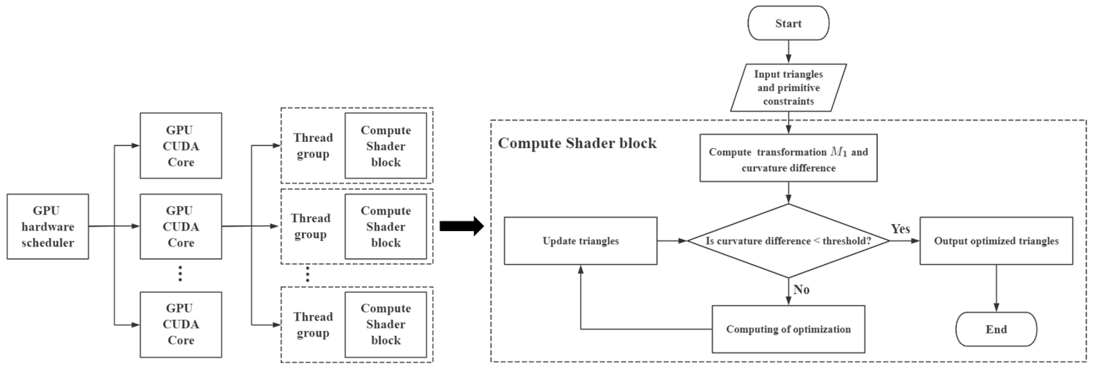
As the size and complexity of the point cloud increase, the memory and computation requirements will grow significantly. To handle these challenges, we propose the use of a memory-efficient data structure and partitioning strategy. Specifically, we divide the point cloud data into smaller and manageable regions, which are processed individually and later stitched together. Additionally, a hierarchical data structure, Octree, is used to manage large-scale point cloud data more effectively. These methods not only reduce memory consumption but also improve processing speed by focusing computations on the loaded point clouds. Furthermore, GPU-based parallelization is employed to accelerate the computation, allowing for more efficient handling of large and complex point clouds. The optimization process is implemented on the GPU using a compute shader framework. Based on the rendering pipeline, our GPU parallel optimization algorithm uploads the input triangles and initial constraint data into GPU buffers. The GPU then creates a grid of thread groups and distributes the buffered data evenly among them. Through the hardware scheduler, each thread group is assigned to available compute cores for parallel execution. Each thread within a group executes the same computational procedure, as illustrated in Figure 5 (Compute Shader block), but processes different subsets of data. After computation, each thread writes its results into a designated read–write buffer for synchronization and subsequent aggregation. This process enables efficient parallel optimization across thousands of mesh elements simultaneously.

4. Experimental Verification

4.1. Original Point Cloud Data and Simplification Result

In this paper, we take the point cloud data of different buildings as examples to show the calculation process of our algorithm. Point cloud data of the single building obtained by point cloud data preprocessing is shown in the first row of Figure 6. The second row of Figure 6 shows the simplification result of each building point cloud.

4.2. Generation of Geometric Primitive

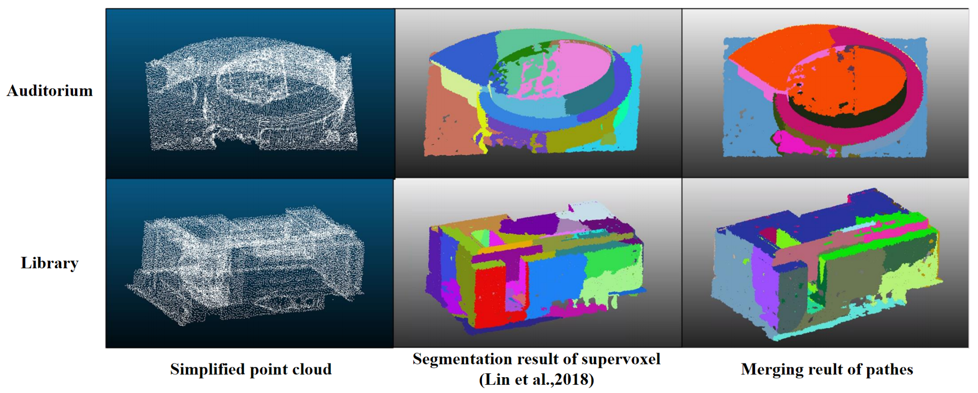
After the data preprocessing of point cloud simplification, we use the supervoxel method [43] to presegment point cloud data. The segmentation result is shown in Figure 7. It can be seen from the second column that the segmentation results well preserve the boundary information. In order to obtain as complete geometric primitives as possible, we merge the obtained segmentation results on the basis of guaranteeing the boundaries. The merging result is shown in the third column of Figure 7.

4.3. Model Optimization Comparison

In order to verify the effectiveness and superiority of our method, we compare our method with Points2surf [22], Polyfit [14], and the classic Screened Poisson Reconstruction method [46]. In the comparison experiment, we first use these three methods to reconstruct the point cloud. The experiments are based on the open-source codes of these three methods, and several parameter adjustments and optimizations have been performed. The schematic diagram of the reconstruction result based on these three methods is shown in Figure 8. The proposed method was coded in C++ and run on the Intel i9-10900K CPU and NVIDIA GeForce RTX 2080 GPU, with 40 GB of memory, on a Windows operating system. The corresponding running time comparison is shown in Table 1. Except for the Points2surf method, which takes more than 1 min on each mesh model, other methods can efficiently achieve mesh model reconstruction. Although the Polyfit method is slightly faster than our method, Polyfit does not obtain valid reconstruction results.
Points2Surf is a patch-based learning framework that generates meshes directly from raw scans without requiring normal information. As shown in Figure 8 (second column), it fails to capture fine structural details, reconstructing only the general shape of the building and exhibiting limited generalization. PolyFit formulates surface reconstruction as a binary labeling problem to recover polygonal meshes from point clouds. However, it is tailored for low-complexity and closed shapes with planar surfaces, making it unsuitable for large-scale or geometrically complex buildings. As seen in Figure 8 (third column), PolyFit fails to reconstruct curved surfaces (rows 1–2) and overfits in some successful cases, generating invalid or over-optimized meshes. The Screened Poisson Surface Reconstruction (SPR) method produces watertight surfaces from oriented point sets, but it suffers from excessive redundant geometry, poor detail fidelity, and rough surfaces. Moreover, its performance is sensitive to manually tuned parameters and is biased toward closed shapes. None of these three methods supports subsequent mesh editing.
Table 2 and Table 3 provide both qualitative and quantitative comparisons of our method against baseline approaches. For qualitative comparison, the evaluation is based on five criteria: visual quality, surface smoothness, detail preservation, structural integrity, and editability (✓ for satisfactory, ✗ for poor performance). During the qualitative evaluation, 20 volunteers participated in the assessment. Our method is the only one that performs well across all categories, demonstrating superior capability in preserving fine geometric features, producing clean and structurally coherent meshes, and supporting subsequent editing. For quantitative comparison, the Chamfer distance results ( × 10 4 ) across four representative datasets further validate our method’s effectiveness. It achieves the lowest distance on three out of four datasets (point cloud 1, point cloud 2, and point cloud 3), with a particularly notable improvement on the “point cloud 3” dataset, where our method attains a distance of just 0.72, far outperforming Point2Surf (39.39) and PolyFit (237.69). Although Point2Surf slightly outperforms ours on the “point cloud 4” dataset, it exhibits inconsistent performance elsewhere. Overall, the results highlight the robustness, precision, and generalizability of our reconstruction pipeline across diverse and complex architectural scenes. The reconstruction accuracy of the proposed method is closely related to the quality of the input point cloud. Higher point density and lower noise levels allow more accurate fitting of geometric primitives, leading to smoother surfaces and better geometric consistency in junction areas. In contrast, sparse or noisy point clouds may cause deviations in segmentation boundaries and introduce errors during optimization. Nevertheless, the geometric primitive constrained optimization maintains stable reconstruction quality under moderate noise, demonstrating good robustness and adaptability to different data qualities. For comparison, the relatively poor performance of PolyFit [14] in our experiments can be attributed to its data quality requirements and algorithmic limitations. PolyFit [14] requires highly preprocessed point clouds with low noise and accurately estimated normals. However, our datasets were obtained directly from real-world scanning without manual denoising or refinement in order to better evaluate robustness. Furthermore, PolyFit [14] reconstructs surfaces by extracting planar primitives and selecting optimal face subsets through global optimization. While this approach is effective for regular and symmetric structures, it becomes less suitable for complex or curved buildings (e.g., the auditorium model used in our tests), where over-segmentation and misfitting of planes may occur, resulting in less realistic surface reconstruction.
Subsequently, we applied our algorithm for reconstruction and surface optimization. The results are illustrated in Figure 9. As observed from the surface optimization results, our method achieves promising performance. The optimized mesh better conforms to the geometric characteristics of the building and exhibits smoother surfaces. The optimization effectively eliminates the roughness present in the initial mesh. Our method is editing-oriented, enabling localized optimization based on specific user requirements. Users can select specific regions and apply varying degrees of optimization to the reconstructed model according to their needs. To further illustrate the specific effects of surface and linear junction area optimization, four representative cases are shown in Figure 10a–d. Figure 10a demonstrates the roof–wall junction optimization, where the linear intersection between the roof planes is refined and redundant facets are removed, resulting in smoother edge continuity; Figure 10b shows the wall–wall junction optimization, in which the alignment between vertical planes is improved and the corner geometry becomes sharper and more consistent; Figure 10c presents the roof curvature junction optimization, where the fitted constraint surface corrects curvature deviations and eliminates uneven transitions in the curved roof region; Figure 10d illustrates a complex multi-surface junction optimization, where both linear and curved surfaces are jointly refined to enhance structural regularity and reduce local surface distortion. These examples highlight the capability of the proposed geometric primitive constrained optimization to accurately handle different junction types and improve overall reconstruction quality.
Point cloud processing methods are often sensitive to point cloud noise, causing the method to succeed on one model but fail on another. In order to solve this problem, we design a spatial sparsity patch statistic method based on the continuity of local geometric features to fix the unsatisfactory point cloud segmentation result and perform the classification calculation of the point cloud patch. Our method has good controllability and adaptability. Moreover, geometric primitive constraints generated in our method have good analytical properties and conform to actual architectural design rules. The entire pipeline is interpretable, and each calculation process has a clear geometric meaning.
As can be seen from the experimental process, the LIDAR point cloud reconstruction method based on geometric primitive constraint proposed in this paper can effectively reconstruct the building point cloud data. The optimized mesh model realizes the description of the real geometric structure of the building. The optimized model is more regular, and the influence of point cloud noise is eliminated. The obtained results can be used for serious applications, such as BIM, CAD design, etc. During the experimental process, we found that the geometric primitive constrained optimization method proposed in this paper can be used to achieve model reconstruction and optimization for large-scale building scenes, such as the unified optimization of regular blocks.
For large-scale scenarios, the memory usage of our method remains relatively constant. Based on the efficient point cloud data structure, the amount of data scheduled into memory remains relatively stable, thus preventing excessive memory consumption. Additionally, we have employed view frustum filtering and a parallel algorithm to further enhance the efficiency. GPU parallel computing is utilized to accelerate the entire process, significantly improving efficiency. When dealing with highly irregular structures, our method will have challenges. Our strategy is adaptable to the precision requirements of the user. For cases with moderate error tolerance, our subdivision algorithm effectively handles the situation, providing satisfactory reconstruction results. However, when higher precision is required, the subdivision algorithm iterates further to meet the accuracy demand, thus requiring more time to complete the reconstruction process. Consequently, for highly irregular structures with high precision demands, our method still requires further optimization to improve computational efficiency.

5. Conclusions

In order to address the problems of low accuracy and the complicated and time-consuming modeling process of the building point cloud reconstruction, this paper proposes a reconstruction method based on geometric primitive constrained optimization. It can be used in serious application scenarios. We design the geometric primitive constrained optimization calculation and conduct experimental tests on LIDAR point cloud data of buildings. On the scanning data set, the algorithm proposed in this paper has achieved good experimental results, which can effectively realize the reconstruction of building LIDAR point clouds, and maintain the geometric accuracy and visual effect.
While the proposed algorithm has shown promising results, it is important to acknowledge certain limitations of the current method. One of the key challenges is the sensitivity to segmentation errors. The accuracy of the reconstruction highly depends on the quality of the initial segmentation, and errors in this step will affect the final model quality. The method’s reliance on clean and accurate thematic data, such as map data or BIM, is also a limitation. In real-world applications, the availability of high-quality thematic data may be limited, which could impact the performance of the algorithm. Moreover, the current geometric primitive constraint framework mainly focuses on predefined shapes such as planes, B-spline surfaces, and linear junctions. These constraints are effective for regular architectural structures but less adaptable to irregular or free-form geometries. In addition, the weighting coefficients in the energy equation are manually determined, which may limit the flexibility and adaptability of the optimization process.
The model optimization calculation method in this paper is based on the geometric primitive constraint, which is also suitable for large-scale scenes. For models that contain a lot of details, more constraints need to be generated. Therefore, for highly irregular structures with high precision demands, our method still requires further optimization to improve computational efficiency. In future work, research will focus on enhancing the constraint adaptability and automation, such as introducing data-driven or adaptive weighting mechanisms, integrating semantic or topological constraints, and developing multi-level optimization strategies for large and complex building scenes. These directions will further improve the robustness, scalability, and practicality of the proposed reconstruction method.

Author Contributions

Conceptualization, T.L., R.S. and H.L.; methodology, T.L. and H.L.; software, R.S.; validation, T.L. and Z.L.; formal analysis, H.L. and T.L.; investigation, Z.L.; resources, T.L.; data curation, T.L. and Z.L.; writing—original draft preparation, H.L. and R.S.; writing—review and editing, H.L. and T.L.; visualization, H.L.; supervision, T.L.; project administration, T.L.; funding acquisition, T.L. All authors have read and agreed to the published version of the manuscript.

Funding

This work was supported by the Open Project Program of the State Key Lab of CAD&CG (Zhejiang University) under grant A2107; funding from State Key Laboratory of Maritime Technology and Safety; and funding from the Hubei Key Laboratory of Inland Shipping Technology under grant NHHY2019001.

Data Availability Statement

The data that support the findings of this study are available from the corresponding author, [T. Liu], upon reasonable request.

Conflicts of Interest

The authors declare that they have no conflicts of interest.

References

  1. Huang, J.; Stoter, J.; Peters, R.; Nan, L. City3D: Large-Scale Building Reconstruction from Airborne LIDAR Point Clouds. Remote Sens. 2022, 14, 2254. [Google Scholar] [CrossRef]
  2. Barnes, D.; Gadd, M.; Murcutt, P.; Newman, P.; Posner, I. The Oxford Radar RobotCar Dataset: A Radar Extension to the Oxford RobotCar Dataset. arXiv 2019, arXiv:1909.01300. [Google Scholar]
  3. Li, Z.; Jie, S. RANSAC-based Multi Primitive Building Reconstruction from 3D Point Clouds. ISPRS J. Photogramm. Remote Sens. 2022, 185, 247–260. [Google Scholar] [CrossRef]
  4. Sun, C.; Miao, L.; Wang, M.; Shi, J.; Ding, J. Research on Point Cloud Hole Filling and 3D Reconstruction in Reflective Area. Sci. Rep. 2023, 13, 18524. [Google Scholar] [CrossRef]
  5. Zabin, A.; González, V.A.; Zou, Y.; Amor, R. Applications of Machine Learning to BIM: A Systematic Literature Review. Adv. Eng. Inform. 2022, 51, 101474. [Google Scholar] [CrossRef]
  6. Pan, X.; Lin, Q.; Ye, S.; Li, L.; Guo, L.; Harmon, B. Deep Learning Based Approaches from Semantic Point Clouds to Semantic BIM Models for Heritage Digital Twin. Herit. Sci. 2024, 12, 65. [Google Scholar] [CrossRef]
  7. Liu, T.; Geng, S.; Fu, Y.; Lei, Z.; Huo, Y.; Zhang, X.; Wang, F.; Han, B.; Sha, M.; Wu, Z. Triplane generator-based NeRF-GAN framework for single-view ship reconstruction. Int. J. Digit. Earth 2025, 18, 2496406. [Google Scholar] [CrossRef]
  8. Liu, T.; Shen, R.; Lei, Z.; Huo, Y.; Zhao, J.; Xu, X. Wind resistance aerial path planning for efficient reconstruction of offshore ship. Int. J. Digit. Earth 2022, 15, 1881–1904. [Google Scholar] [CrossRef]
  9. Shen, W.; Li, J.; Chen, Y.; Deng, L.; Peng, G. Research on Building Contour Extraction and Regularization Algorithm Based on LIDAR Data. J. Remote Sens. 2008, 12, 692–698. [Google Scholar]
  10. Yang, L.; Sheng, Y.; Wang, B. LIDAR Data Reduction Assisted by Optical Image for 3D Building Reconstruction. Optik 2014, 125, 6282–6286. [Google Scholar] [CrossRef]
  11. Li, L.; Song, N.; Sun, F.; Liu, X.; Wang, R.; Yao, J.; Cao, S. Point2Roof: End-to-end 3D Building Roof Modeling from Airborne LIDAR Point Clouds. ISPRS J. Photogramm. Remote Sens. 2022, 193, 17–28. [Google Scholar] [CrossRef]
  12. Bourki, A.; de La Gorce, M.; Marlet, R.; Komodakis, N. Patchwork Stereo: Scalable, Structure-Aware 3D Reconstruction in Man-Made Environments. In Proceedings of the 2017 IEEE Winter Conference on Applications of Computer Vision (WACV), Santa Rosa, CA, USA, 24–31 March 2017; pp. 292–301. [Google Scholar]
  13. Lan, Z.; Yew, Z.J.; Lee, G.H. Robust Point Cloud Based Reconstruction of Large-Scale Outdoor Scenes. In Proceedings of the IEEE Conference on Computer Vision and Pattern Recognition, Long Beach, CA, USA, 15–20 June 2019; pp. 9690–9698. [Google Scholar]
  14. Nan, L.; Wonka, P. Polyfit: Polygonal Surface Reconstruction from Point Clouds. In Proceedings of the IEEE International Conference on Computer Vision, Venice, Italy, 22–29 October 2017; pp. 2353–2361. [Google Scholar]
  15. Nan, L.; Xie, K.; Sharf, A. A Search-Classify Approach for Cluttered Indoor Scene Understanding. ACM Trans. Graph. (TOG) 2012, 31, 1–10. [Google Scholar] [CrossRef]
  16. Shao, T.; Xu, W.; Zhou, K.; Wang, J.; Li, D.; Guo, B. An Interactive Approach to Semantic Modeling of Indoor Scenes with an RGBD Camera. ACM Trans. Graph. (TOG) 2012, 31, 136:1–136:11. [Google Scholar] [CrossRef]
  17. Verdie, Y.; Lafarge, F.; Alliez, P. Lod Generation for Urban Scenes. ACM Trans. Graph. (TOG) 2015, 34, 30. [Google Scholar] [CrossRef]
  18. Xu, K.; Zheng, H.; Zhang, H.; Cohen-Or, D.; Liu, L.; Xiong, Y. Photo-Inspired Model-Driven 3D Object Modeling. ACM Trans. Graph. (TOG) 2011, 30, 1–10. [Google Scholar]
  19. Shen, C.-H.; Fu, H.; Chen, K.; Hu, S.-M. Structure Recovery by Part Assembly. ACM Trans. Graph. (TOG) 2012, 31, 1–11. [Google Scholar] [CrossRef]
  20. Wu, Z.; Wang, X.; Lin, D.; Lischinski, D.; Cohen-Or, D.; Huang, H. Sagnet: Structure-Aware Generative Network for 3D-Shape Modeling. ACM Trans. Graph. (TOG) 2019, 38, 1–14. [Google Scholar] [CrossRef]
  21. Dai, A.; Nießner, M. Scan2mesh: From Unstructured Range Scans to 3D Meshes. In Proceedings of the IEEE/CVF Conference on Computer Vision and Pattern Recognition, Long Beach, CA, USA, 15–20 June 2019; pp. 5574–5583. [Google Scholar]
  22. Erler, P.; Guerrero, P.; Ohrhallinger, S.; Mitra, N.J.; Wimmer, M. Points2surf Learning Implicit Surfaces From Point Clouds. In Proceedings of the 2020 European Conference on Computer Vision, Glasgow, UK, 23–28 August 2020; pp. 108–124. [Google Scholar]
  23. Sun, J.; Chen, X.; Wang, Q.; Li, Z.; Averbuch-Elor, H.; Zhou, X.; Snavely, N. Neural 3D Reconstruction in the Wild. In Proceedings of the ACM SIGGRAPH 2022 Conference Proceedings, Vancouver, BC, Canada, 7–11 August 2022. [Google Scholar]
  24. Monszpart, A.; Mellado, N.; Brostow, G.J.; Mitra, N.J. RAPter: Rebuilding Man-Made Scenes with Regular Arrangements of Planes. ACM Trans. Graph. (TOG) 2015, 34, 103:1–103:12. [Google Scholar] [CrossRef]
  25. Musialski, P.; Wonka, P.; Aliaga, D.G.; Wimmer, M.; Van Gool, L.; Purgathofer, W. A Survey of Urban Reconstruction. Comput. Graph. Forum 2013, 32, 146–177. [Google Scholar] [CrossRef]
  26. Zheng, Q.; Sharf, A.; Wan, G.; Li, Y.; Mitra, N.J.; Cohen-Or, D.; Chen, B. Non-Local Scan Consolidation for 3D Urban Scenes. ACM Trans. Graph. (TOG) 2010, 29, 94:1–94:9. [Google Scholar] [CrossRef]
  27. Nan, L.; Sharf, A.; Zhang, H.; Cohen-Or, D.; Chen, B. Smartboxes for Interactive Urban Reconstruction. ACM Trans. Graph. (TOG) 2010, 29, 93:1–93:10. [Google Scholar] [CrossRef]
  28. Li, Y.; Zheng, Q.; Sharf, A.; Cohen-Or, D.; Chen, B.; Mitra, N.J. 2D-3D Fusion for Layer Decomposition of Urban Facades. In Proceedings of the 2011 International Conference on Computer Vision, Barcelona, Spain, 6–13 November 2011; pp. 882–889. [Google Scholar]
  29. Arikan, M.; Schwärzler, M.; Flöry, S.; Wimmer, M.; Maierhofer, S. O-Snap: Optimization-Based Snapping for Modeling Architecture. ACM Trans. Graph. (TOG) 2013, 32, 6:1–6:15. [Google Scholar] [CrossRef]
  30. Lafarge, F.; Alliez, P. Surface Reconstruction Through Point Set Structuring. Comput. Graph. Forum 2013, 32 Pt 2, 225–234. [Google Scholar] [CrossRef]
  31. Lin, H.; Gao, J.; Zhou, Y.; Lu, G.; Ye, M.; Zhang, C.; Liu, L.; Yang, R. Semantic Decomposition and Reconstruction of Residential Scenes from LIDAR Data. ACM Trans. Graph. (TOG) 2013, 32, 66:1–66:10. [Google Scholar] [CrossRef]
  32. Li, M.; Wonka, P.; Nan, L. Manhattan-World Urban Reconstruction from Point Clouds. In Proceedings of the European Conference on Computer Vision, Amsterdam, The Netherlands, 11–14 October 2016; pp. 54–69. [Google Scholar]
  33. Zhang, L.; Li, Z.; Li, A.; Liu, F. Large-Scale Urban Point Cloud Labeling and Reconstruction. ISPRS J. Photogramm. Remote Sens. 2018, 138, 86–100. [Google Scholar] [CrossRef]
  34. Li, M.; Rottensteiner, F.; Heipke, C. Modelling of Buildings from Aerial LIDAR Point Clouds Using TINs and Label Maps. ISPRS J. Photogramm. Remote Sens. 2019, 154, 127–138. [Google Scholar] [CrossRef]
  35. Albano, R. Investigation on Roof Segmentation for 3D Building Reconstruction from Aerial LIDAR Point Clouds. Appl. Sci. 2019, 9, 4674. [Google Scholar] [CrossRef]
  36. Dong, W.; Park, J.; Yang, Y.; Kaess, M. GPU Accelerated Robust Scene Reconstruction. In Proceedings of the 2019 IEEE/RSJ International Conference on Intelligent Robots and Systems (IROS), Macau, China, 3–8 November 2019. [Google Scholar]
  37. Wang, R.; Peethambaran, J.; Chen, D. LIDAR Point Clouds to 3-D Urban Models: A Review. IEEE J. Sel. Top. Appl. Earth Obs. Remote Sens. 2018, 11, 606–627. [Google Scholar] [CrossRef]
  38. Jiang, R. Building Model Reconstruction Based on the Technology of 3D Laser Scanning. Bull. Surv. Mapp. 2013, S1, 80–83+120. [Google Scholar]
  39. Rusu, R.B.; Cousins, S.B. 3D is here: Point Cloud Library (PCL). In Proceedings of the 2011 IEEE International Conference on Robotics and Automation, Shanghai, China, 9–13 May 2011; pp. 1–4. [Google Scholar]
  40. Li, B.J.; Li, Q.Q.; Shi, W.Z.; Wu, F.F. Feature Extraction and Modeling of Urban Building from Vehicle-Borne Laser Scanning Data. Int. Arch. Photogramm. Remote Sens. Spat. Inf. Sci. 2004, 35, 934–939. [Google Scholar]
  41. Milioto, A.; Vizzo, I.; Behley, J.; Stachniss, C. Rangenet++: Fast and accurate LIDAR semantic segmentation. In Proceedings of the 2019 IEEE/RSJ International Conference on Intelligent Robots and Systems (IROS), Macau, China, 3–8 November 2019; pp. 4213–4220. [Google Scholar]
  42. Kuo, C.-C.; Yau, H.-T. A Delaunay-based Region-growing Approach to Surface Reconstruction from Unorganized Points. Comput.-Aided Des. 2005, 37, 825–835. [Google Scholar] [CrossRef]
  43. Lin, Y.; Wang, C.; Zhai, D.; Li, W.; Li, J. Toward Better Boundary Preserved Supervoxel Segmentation for 3D Point Clouds. ISPRS J. Photogramm. Remote Sens. 2018, 143, 39–47. [Google Scholar] [CrossRef]
  44. Liu, T.; Zhao, D.; Pan, M. An Approach to 3D Model Fusion in GIS Systems and Its Application in A Future ECDIS. Comput. Geosci. 2016, 89, 12–20. [Google Scholar] [CrossRef]
  45. Laine, S.; Karras, T. High-Performance Software Rasterization on GPUs. In Proceedings of the ACM SIGGRAPH Symposium on High Performance Graphics, Vancouver, BC, Canada, 5–7 August 2011; pp. 79–88. [Google Scholar]
  46. Kazhdan, M.M.; Hugues, H. Screened poisson surface reconstruction. ACM Trans. Graph. 2013, 32, 29:1–29:13. [Google Scholar] [CrossRef]
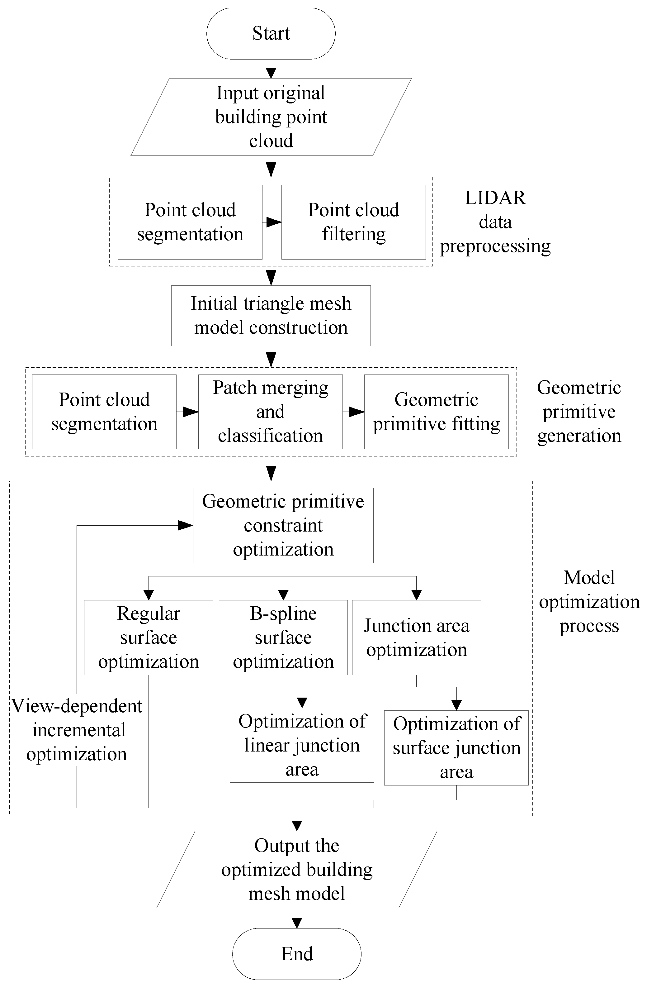
Figure 1. The flowchart of the whole algorithm. The algorithm processes raw building point clouds through segmentation, mesh construction, and multi-stage geometric optimization. It applies surface fitting, primitive constraints, and view-dependent refinement to generate an accurate building mesh model.
Applsci 15 11286 g001
Figure 2. The flowchart of the patch merging algorithm. This algorithm takes two point cloud patches as input and merges them through a sequence of steps. It begins by generating KD-trees to efficiently search for K nearest neighbors. Boundary points are identified and analyzed for local geometric features such as mean normal vectors and curvature. A threshold-based decision process, combined with distance checks and cross-validation, determines whether the patches can be merged.
Applsci 15 11286 g002
Figure 3. The flowchart of the patch classification algorithm. This algorithm classifies a point cloud patch by first computing its oriented bounding box (OBB), segmenting the bounding box into blocks, and analyzing local geometric features such as normal vectors.
Applsci 15 11286 g003
Figure 4. The flowchart of geometric primitive constraint-based model optimization. This process integrates thematic information with point cloud data through pose adjustment and scale transformation, iteratively optimizing under geometric constraints until convergence is reached.
Applsci 15 11286 g004
Figure 5. The flowchart of the parallel algorithm. This algorithm performs parallel optimization on input triangles under given constraints. It iteratively checks if the optimization condition is met and outputs the optimized triangles once satisfied.
Applsci 15 11286 g005
Figure 6. Schematic diagram of the original point cloud data and simplification result. The point cloud data was composed of real-world point cloud data acquired from four campus buildings: an auditorium, a library, a student services center, and a teaching building.
Applsci 15 11286 g006
Figure 7. The results of segmentation and merging. We use the supervoxel method [43] to obtain the segmentation results, and then utilized the boundary information contained within these segmentation results to merge them.
Applsci 15 11286 g007
Figure 8. The reconstruction results of Point2surf [22], Polyfit [14], and SPR [46] in four different buildings. In order to highlight the advantages of the proposed method, the reconstruction results of the proposed method for four distinct building types are presented separately in Figure 9.
Applsci 15 11286 g008
Figure 9. The reconstruction result of our method. As can be observed in the figure, our reconstruction demonstrates superior quality compared to the methods presented in Figure 8. Furthermore, the optimized results exhibit enhanced surface connectivity and smoothness.
Applsci 15 11286 g009
Figure 10. Optimization results for representative junction areas. The optimization effectively refines both surface and junction areas, demonstrating the capability of the geometric primitive constrained optimization to enhance reconstruction accuracy and visual quality.
Applsci 15 11286 g010
Table 1. Runtime performance of the different reconstruction methods (best, i.e., lowest, times in bold).
DatasetTime in Seconds ↓
Points2Surf PolyFit SPR Ours
Point cloud 193.161.847.167.63
Point cloud 272.843.544.394.51
Point cloud 3102.473.387.577.99
Point cloud 478.376.876.607.01
Table 2. Subjective evaluation results of different reconstruction methods (✓: good performance, ✗: average or poor performance).
CriterionPoints2SurfPolyFitSPROurs
Visual quality
Surface smoothness
Detail preservation
Structural integrity
Editability
Table 3. Chamfer distance (in 10 4 ) of different reconstruction methods on various datasets (best values in bold). ↓ indicates that the lower the chamfer distance evaluation metric, the better the method’s performance.
DatasetChamfer Distance ( × 10 4 ) ↓
Point2Surf PolyFit SPR Ours
Point cloud 14.17128.1741.321.04
Point cloud 217.5488.81130.565.03
Point cloud 339.39237.69128.500.72
Point cloud 41.8040.94183.906.59
Disclaimer/Publisher’s Note: The statements, opinions and data contained in all publications are solely those of the individual author(s) and contributor(s) and not of MDPI and/or the editor(s). MDPI and/or the editor(s) disclaim responsibility for any injury to people or property resulting from any ideas, methods, instructions or products referred to in the content.