Hybrid Methodological Evaluation Using UAV/Satellite Information for the Monitoring of Super-Intensive Olive Groves

Abstract

Advances in Earth observation technology using multispectral imagery from satellite Earth observation systems and sensors mounted on unmanned aerial vehicles (UAVs) are enabling more accurate crop monitoring. These images, once processed, facilitate the analysis of crop health by enabling the study of crop vigour, the calculation of biomass indices, and the continuous temporal monitoring using vegetation indices (VIs). These indicators allow for the identification of diseases, pests, or water stress, among others. This study compares images acquired with the Altum PT sensor (UAV) and Super Dove (satellite) to evaluate their ability to detect specific problems in super-intensive olive groves at two critical times: January, during pruning, and April, at the beginning of fruit development. Four different VIs were used, and multispectral maps were generated for each: the Normalized Difference Vegetation Index (NDVI), the Green Normalized Difference Vegetation Index (GNDVI), the Normalized Difference Red Edge Index (NDRE) and the Leaf Chlorophyll Index (LCI). Data for each plant (n = 11,104) were obtained for analysis across all dates and sensors. A combined methodology (Spearman’s correlation coefficient, Student’s t-test and decision trees) was used to validate the behaviour of the variables and propose predictive models. The results showed significant differences between the sensors, with a common trend in spatial patterns and a correlation range between 0.45 and 0.68. Integrating both technologies enables multiscale assessment, optimizing agronomic management and supporting more sustainable precision agriculture.

1. Introduction

The monitoring of woody crops, particularly olive groves, has made significant progress due to the use of remote sensors and the analysis of their multispectral images [1]. The use of remote sensing and multispectral image analysis provides an innovative and accurate approach to assessing crop condition and development in a non-destructive way, enabling real-time decision-making and optimisation of agricultural resources [2,3,4]. In recent years, the incorporation of satellite and unmanned aerial vehicle (UAV) imagery has become popular, providing complementary solutions for the analysis of large crop areas, wide coverage with high temporal frequency (satellites) and higher spatial resolution for localised detection (UAVs) and detailed assessment at plant level [5,6].

The present study proposes a hybrid methodological assessment, understood as the integration of multi-source data, satellite and UAV, through statistical, spatial and predictive analyses, with the aim of ensuring the scalability and statistical validation of the results, so that the metrics obtained at tree level can be reliably extrapolated to the plot and farm scales [7]. This transferability constitutes an innovative contribution in comparison to previous studies that focused on herbaceous crops or single-source analysis [8,9].

The main challenge in integrating data from multiple sources is the variation in observation scales and spatial and spectral resolutions [10,11]. This complementarity is particularly relevant in super-intensive olive groves, where UAVs’ ability to capture intra-plot variability and critical plant level phenomena complements the satellites’ ability to monitor regional trends.

Multispectral imaging allows for the measurement of electromagnetic energy re-emitted by plants at different wavelengths across the spectrum. These measurements vary according to the physical properties of the vegetation, producing reflectance curves that are key to identifying plant health and vigour [12].

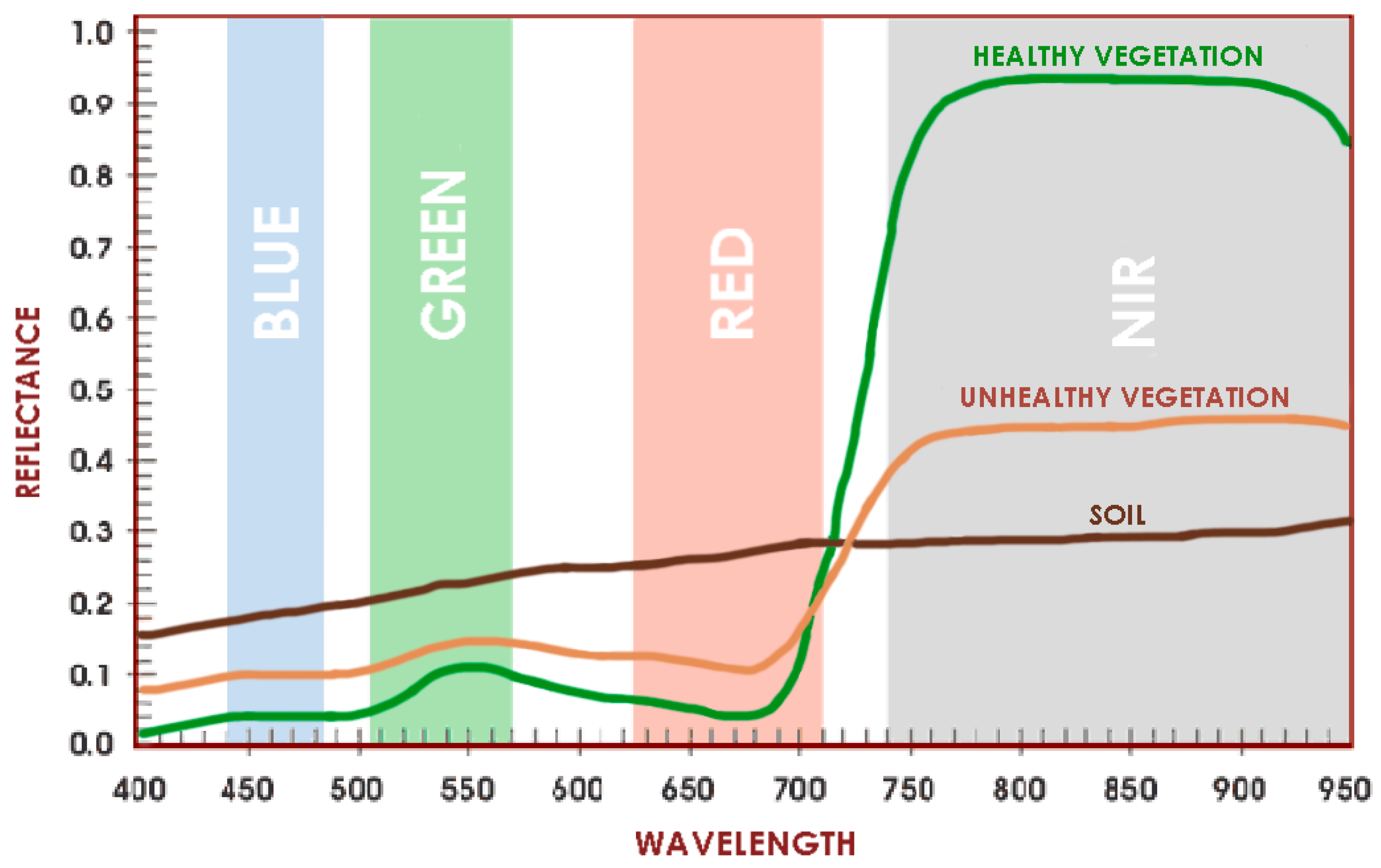
Healthy vegetation (Figure 1) shows a minimum of reflectance in the visible spectrum (400–700 nm), with a peak of reflected energy in the green band at 500–600 nm, known as the ‘green bulge’ of healthy vegetation. The Red Edge (700–730 nm) is a sensitive indicator of plant stress, as a stressed plant exhibits very low reflectance in this band. In the Near-Infrared Spectroscopy (NIR) band (700–1400 nm), reflectance increases dramatically in healthy vegetation, and monitoring this is a way of determining how healthy a crop is, since stressed vegetation reflects significantly less in the infrared range. Similar to the red spectral band, the infrared range is widely used to calculate most vegetation indices in agriculture [13].

The use of sensors onboard UAVs enables a much higher spatial resolution than satellite imagery, allowing a detailed representation of each plant and facilitating the detection of local variations in the crop. However, the higher spatial resolution of UAVs must be balanced against the limited temporal coverage of satellites, which provide images of large areas at lower resolution but are useful for large-scale trend analysis.

This research focuses on the olive crops grown under super-intensive management, whose linear and homogenous structure allows a good response to remote image-based segmentation. This study focuses on olives due to their significant economic importance in the Mediterranean region, as well as their distinct phenology, which allows for the identification of critical assessment periods using VL.

Remote sensing offers specific advantages and contributions when applied to perennial woody crops such as olive trees, compared to annual crops. This is because it allows us to address the challenges posed by olives’ complex canopy structure and long life cycles, as well as the need for multi-year monitoring of their response to pruning and management practices [14,15]. In this context, the combination of UAV and satellite imagery not only improves the detection of variability within plots and across regions but also helps overcome two critical limitations of agricultural remote sensing: the scalability of analyses and the statistical validation of predictive models. This ensures that results can be transferred from the plant scale to the farm scale. The need for scalability and validation has been identified as an area of research that remains underexplored in the literature on woody crop applications.

This multiscale approach is particularly novel in super-intensive olive groves [7,9]. The periods selected for this study (January, when pruning defines the potential for sprouting and yield for the season, and April, when the foundations for production are laid through sprouting and fruit set) represent critical phenological phases in olive tree management. Accurate monitoring in these phases allows for the efficient adjustment of irrigation, fertilisation and pruning practices, as these determine annual productivity and crop sustainability [16,17].

While previous studies have explored the use of remote sensing for herbaceous crops such as maize and wheat, fewer studies have focused on woody crops, particularly super-intensive olive groves [18,19,20]. Some studies have shown that the Normalized Difference Red Edge Index (NDRE) index obtained by UAVs can detect irrigation non-uniformity in olive groves [21], while others applied high-resolution UAV images for 3D canopy reconstruction [22]. However, few studies have proposed the integration of UAV/satellite data in high-density contexts. One such example is the study by Bollas et al. [23], which evaluated the NDVI obtained from both UAV imagery and Sentinel-2 satellite data in northern Greece, achieving correlations ranging from 83.5% to 98.3%. This demonstrates the value of UAVs in detecting intra-plot variability that is not visible in satellite images.

Therefore, this study proposes a hybrid methodological assessment that not only compares sensors but also proposes combined spatial and temporal analysis models. This hybrid approach integrates comparative statistical analysis, predictive modelling and geospatial segmentation for the generation of management zones. The aim is to overcome the limitations of single-source approaches and provide transferable tools for other perennial agricultural systems. The approach also addresses the lack of scalability and statistical validation in multi-source analysis, supporting more accurate and sustainable agronomic decision-making, with the goal of maximising productivity while reducing environmental impact [24,25,26].

While some recent studies have addressed the spatial segmentation of individual trees in olive cultivation using UAV imagery, such as the work of Safonova et al. [27], which focused on canopy volume estimation, no research has been found that explicitly combines UAV, satellite and predictive modelling to generate management zoning, which constitutes the novel contribution of this study [28,29].

2. Materials and Methods

The main technological advance in the monitoring of woody crops has been the adoption of multispectral imagery [30,31] obtained via drone and satellite flights. In this study, the data obtained from both types of flights and sensors were compared, considering that they have different technical characteristics and flight conditions.

Two specific sensors were used in this study: Planet Lab’s Super-Dove multispectral sensor (Plant Labs PBC, San Francisco, CA, USA) [32] for the satellite imagery and the Altum PT sensor (Micasense; AgEagle Aerial Systems, Wichita, KS, USA) onboard the DJI Matrice 300 RTK drone (https://enterprise.dji.com) (DJI; SZ DJI Technology Co., Ltd., Shenzhen, China) for the UAV imagery.

Satellite images (eight bands) and UAV images (Altum PT, 5 + 1 bands) were obtained using different spectral ranges (Figure 2). In addition to the comparative analysis of the aforementioned bands, the combination of the spectral bands was carried out by means of vegetation indices (VIs), which allowed us to quantify the variability in the crop plots and carry out a geospatial analysis for crop monitoring [33,34].

2.1. Location of the Research

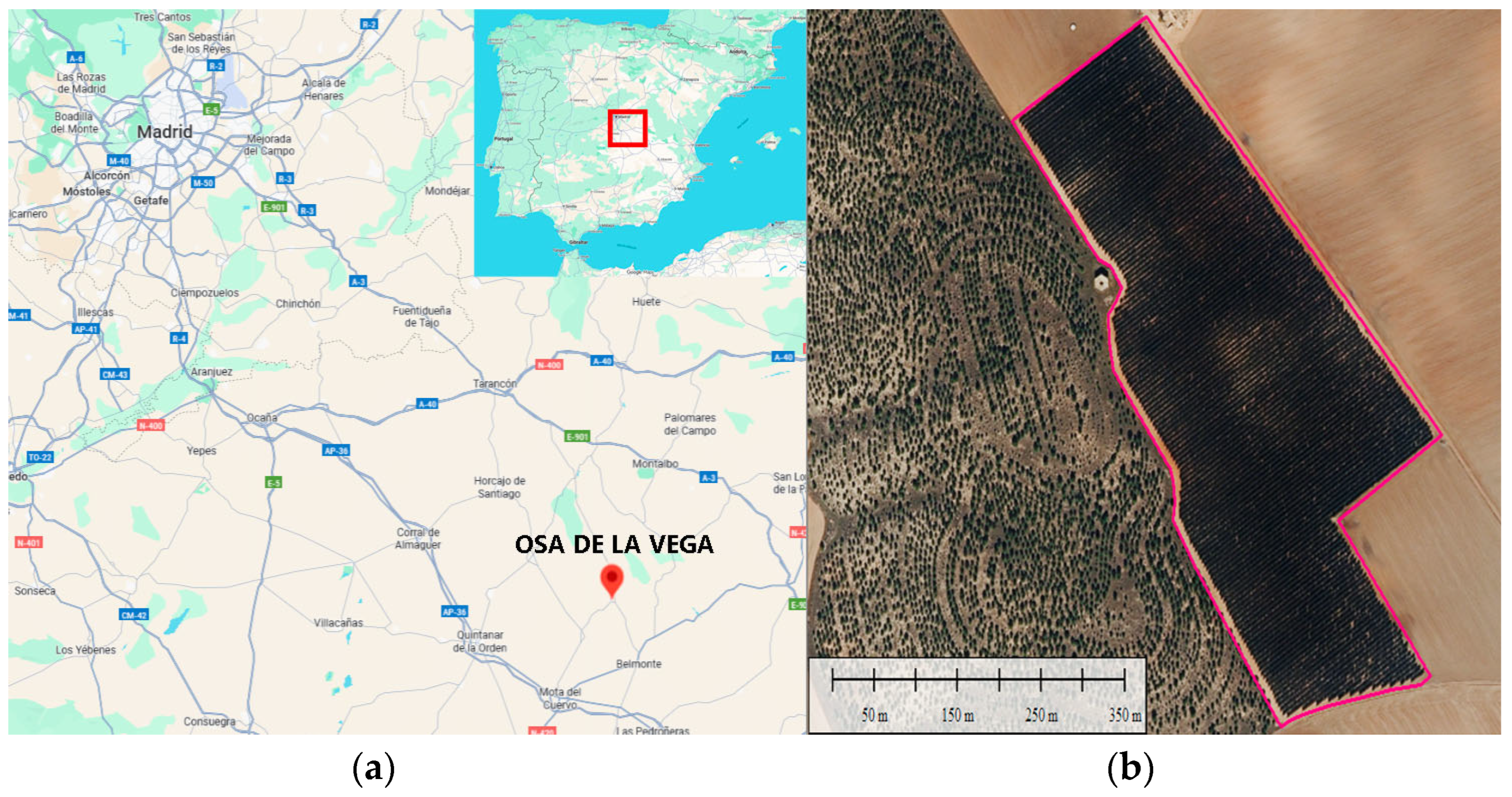
This study was carried out in a super-intensive olive plantation (Cornicabra variety) in Osa de la Vega, Cuenca, Spain (39°40.2′79″ N, 2°42′44.02″ W). The farm has an area of 10 hectares containing 11,104 trees distributed in rows, with a distance of 3.5 m between rows and 1.25–1.5 m between trees (Figure 3). This layout is designed for intensive mechanisation and high productivity [35,36].

The plantation is located on practically flat terrain with a slope of less than 3%. The soil is a mixture of limestone and loam. Although the soil contains a lot of stones, it is of medium fertility and has good drainage. All the trees are the same age (eight years old at the time of this study) and are managed using controlled deficit drip irrigation and annual mechanical pruning. This ensures uniform vegetative development and improves the representativeness of the data.

2.2. Data Collection

The main resource for analysis in this study was multispectral imagery. For the satellite case, daily images are available for download from the satellite provider’s website. However, in the case of the UAV, monthly flights have been carried out since January 2023. From these, two key phenological dates were selected for the year 2023: 29 January and 15 April, corresponding to the rest/pruning and budbreak/flowering stages, respectively. These dates coincide with relevant phenological phases for detecting changes in olive tree vigour and photosynthetic activity [37]. From an agronomic point of view, these phases are critical because they determine key management practices. In January, pruning regulates canopy load and defines the cycle’s potential productivity. In April, budding and flowering determine the yield by influencing both fruit set and competition for resources. From a methodological perspective, these extreme stages of the cycle allow us to validate the ability of UAVs and satellites to detect well-defined physiological contrasts, such as minimal vegetative activity during dormancy, compared to maximum leaf expansion during flowering. This approach strengthens the reliability of the comparison between sensors, as their responses are evaluated in both low- and high-vigour situations. These conditions represent the limits of the spectral range in olive trees, ensuring that the results can be transferred to other contexts more easily.

The satellite images were obtained via direct download from Planet’s own website, Ortho Analytic 8B SR (www.planet.com). The images from Planet are provided with geometric and radiometric corrections already applied to minimise atmospheric distortion [38,39,40,41]. The images are acquired by Planet Lab’s SuperDove sensors (Planet Labs PBC, San Francisco, CA, USA), with a resolution of 3.7 m/pixel and 8 spectral bands: R, G, B, NIR, Coastal Blue, Green, Yellow and Red Edge [32].

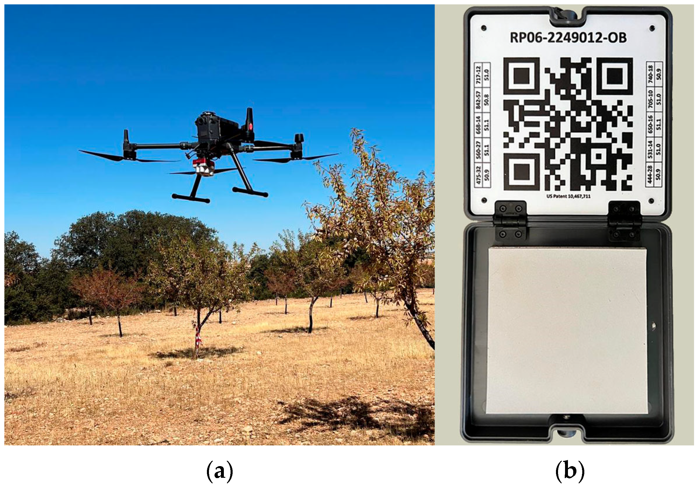
However, the images obtained via UAV flight were acquired using photogrammetric techniques using the Altum PT multispectral sensor onboard the DJI Matrice 300 RTK drone (

Table 1. Basic specifications of the DJI Matrice 300 RTK UAV.

Weight	Approx. 6.3 kg (with One Gimbal)
Max. transmitting distance	8 km
Max. flight time	40 min
Dimensions	810 × 670 × 430 mm
Max. payload	2.7 kg
Max. speed	70 km/h
GNSS	GPS+ GLONASS+ BeiDou+ Galileo
RTK positioning accuracy	1 cm + 1 ppm (horizontal) 1.5 cm + 1 ppm (vertical)

and Figure 4). This camera allows a spatial resolution of 4 cm when flying at an altitude of 120 m thanks to the pansharpening of the panchromatic band. For this work, the drone was flown at an altitude of 70 m, achieving a ground sample distance (GSD) of 2.3 cm/pixel in 4 + 1 bands: R, G, B, Red Edge and IR. The drone was configured to fly with a 75% overlap on the lateral and frontal axes to ensure full coverage. This type of flight with multispectral cameras requires the acquisition of calibration panels to subsequently correct reflectance values and achieve uniformity when comparing flights on different dates and in different weather conditions.

The working area was georeferenced by measuring four points coinciding with the corners of the crop field using a GNSS Zenith 40 device (Geomax AG, Widnau, St. Gallen, Switzerland).

2.3. Methodology

The first phase of satellite data acquisition consisted of downloading Level III images from Planet’s web platform (www.planet.com). As previously indicated in Section 2, the drone flights recorded data on SD cards housed in the multispectral sensor.

In contrast to the satellite images, which are adjusted for reflectance in the download, the photogrammetric flight images had to be processed. This was carried out using Pix4D Mapper software (version 4.9.0), (www.pix4d.com).

Pix4D Mapper made it possible to insert the coordinates of the Ground Control Points (GCPs) obtained from the RTK observations (

Table 2. GCP accuracy in meters (m) using 4 support points.

	X	Y	Z
Mean (m)	0.006	0.007	0.022
Standard deviation (m)	0.007	0.009	0.087
RMS error (m)	0.010	0.011	0.090

), to carry out the pansharpening process in order to obtain the specified resolution and to radiometrically correct the images using the DLS system [42,43,44,45]. The following products were obtained: point clouds, DSMs and orthophotos for each sensor band, from which the different vegetation indices were subsequently calculated. The orthophotos are the result of geometrically correcting the aerial photographs. The orthophotos have a constant scale, and the points indicate accurate geographical positions.

In order to carry out a statistical study of the subject area, the difference between the images was evaluated by comparing the averages (calculated for each individual image) for each of the four VIs: the Normalized Difference Vegetation Index (NDVI), the Green Normalized Difference Vegetation Index (GNDVI), the Normalized Difference Red Edge Index (NDRE) and the Leaf Chlorophyll Index (LCI) [46]. For each of the 11,104 trees, data were obtained for the four VIs on each of the selected dates: 29 January and 15 April 2023, i.e., 44,416 statistical values were obtained for analysis.

These indices were selected for their ability to characterise different physiological aspects of the crop, such as vigour, biomass, chlorophyll content and photosynthetic activity, at critical stages. Previous studies on olive groves have demonstrated the usefulness of the NDRE index for detecting irrigation heterogeneities [21], and the consistency of the NDVI index in UAV–satellite comparisons [23]. Meanwhile, research on other crops has shown that these indices are effective in segmenting and monitoring management areas [47].

From the processing of the orthophotos, the values of reflectance in the different bands of the electromagnetic spectrum were obtained. By combining these bands, the following vegetation indices were obtained [31,47,48,49,50,51]:

NDVI [52,53,54]: this index estimates the vegetation value by combining the NIR and red bands.

NDRE: this index is a useful indicator for analysing biomass during the ripening stage [21,55].

LCI: this index assesses chlorophyll [56,57,58]:

GNDVI: this index assesses photosynthetic activity at advanced stages of the plant cycle [59,60,61,62].

These indices were calculated from calibrated reflectances. In the case of UAVs, images were processed with Pix4D Mapper to generate georeferenced orthomosaics; their resolution was then adjusted to 3 m/pixel to allow direct comparison with Planet imagery. For the satellite images, processing was performed in QGIs Desktop 3.40.8 by selecting specific bands for each index.

This resampling method used block averaging, whereby each satellite pixel (3 × 3 m) acted as a reference polygon, and the average value of all the UAV pixels within it was calculated. This equated each satellite pixel to an average polygon derived from the UAV, ensuring spatial consistency between the two resolutions. This technique was chosen for its ability to preserve average radiometric information and avoid spectral biases when comparing the two resolutions, as well as to ensure spatial consistency.

Following this process, the values corresponding to each individual tree (n = 11,104) were extracted, yielding a total of 88,832 data points per date. These values formed the basis of subsequent statistical analyses, including Spearman’s correlation, Student’s t-test and predictive models.

At the individual tree analysis level, a vector grid was used to segment each of the 11,104 olive trees in the grove. This allowed the extraction of mean index values per individual tree for both dates and sensors. These values are summarized in Appendix A (

Table A1. Mean values of the different VIs (NDVI, NDRE, LCI, GNDVI) measured for each of the 11,104 individual trees in the plot on 15 April 2023.

	Centroid Coord		DRON				Planet
ID	Χ	Y	NDVl	LCI	NDRE	GNDVl	NDVI	LCI	NDRE	GNDVl
			Mean	Mean	Mean	Mean	Mean	Mean	Mean	Mean
1	524,656.5	4,390,903.5	0.1947	0.1161	0.1074	0.4084	0.3652	0.2297	0.2023	0.4433
2	524,659.5	4,390,903.5	0.2953	0.1474	0.1234	0.4512	0.3696	0.2391	0.2115	0.452
3	524,650.5	4,390,900.5	0.5145	0.3339	0.3397	0.5139	0.4763	0.3962	0.3668	0.5199
4	524,653.5	4,390,900.5	0.6217	0.432	0.3612	0.5945	0.4834	0.3612	0.3219	0.5043
5	524,656.5	4,390,900.5	0.4634	0.3042	0.2596	0.5208	0.4936	0.3818	0.3419	0.5285
6	524,659.5	4,390,900.5	0.2646	0.1388	0.1221	0.4353	0.4394	0.2893	0.2516	0.4887
7	524,662.5	4,390,900.5	0.3526	0.1721	0.1403	0.4821	0.4105	0.2754	0.2426	0.4813
8	524,647.5	4,390,897.5	0.5912	0.4352	0.3761	0.5691	0.5207	0.4628	0.4375	0.5741
9	524,650.5	4,390,897.5	0.7153	0.5031	0.4136	0.6855	0.5567	0.4602	0.4197	0.5864
10	524,653.5	4,390,897.5	0.7308	0.5311	0.4423	0.7092	0.5984	0.4787	0.4275	0.6072
11	524,656.5	4,390,897.5	0.7483	0.5266	0.4312	0.7168	0.5906	0.4924	0.4484	0.609
12	524,659.5	4,390,897.5	0.4316	0.3072	0.2602	0.5396	0.51	0.3778	0.3337	0.5451
13	524,662.5	4,390,897.5	0.2447	0.1225	0.1078	0.4337	0.4502	0.3154	0.2779	0.5145
14	524,665.5	4,390,897.5	0.2735	0.1261	0.1067	0.4385	0.4028	0.2875	0.2578	0.5007
15	524,641.5	4,390,894.5	0.5866	0.4301	0.3722	0.5668	0.5359	0.4157	0.3711	0.6008
16	524,644.5	4,390,894.5	0.6541	0.4696	0.3959	0.6235	0.5937	0.4612	0.4073	0.6275
17	524,647.5	4,390,894.5	0.7547	0.5476	0.4537	0.7251	0.6576	0.5209	0.4583	0.6603
18	524,650.5	4,390,894.5	0.7351	0.5242	0.433	0.7173	0.639	0.5218	0.467	0.6442
19	524,653.5	4,390,894.5	0.734	0.5122	0.4186	0.7154	0.637	0.5119	0.455	0.6346
20	524,656.5	4,390,894.5	0.7515	0.554	0.4627	0.7234	0.6296	0.5043	0.4481	0.6262
21	524,659.5	4,390,894.5	0.7433	0.5255	0.4316	0.716	0.5794	0.4484	0.3964	0.5898
22	524,662.5	4,390,894.5	0.4043	0.2404	0.2054	0.5245	0.5225	0.3337	0.3369	0.5666
23	524,665.5	4,390,894.5	0.2066	0.0973	0.0871	0.4235	0.4575	0.321	0.2825	0.5409
24	524,638.5	4,390,891.5	0.6226	0.4585	0.3937	0.6033	0.5956	0.4302	0.3691	0.6044
25	524,641.5	4,390,891.5	0.7236	0.5139	0.4243	0.6878	0.6354	0.5002	0.4406	0.6419

), which presents the complete descriptive statistics used for the comparative analyses between sensors.

Once the statistics were obtained for each individual tree (88,832 per date), different study methods were used to assess the differences between the images, including correlation analyses, mean comparison tests and regression analyses using IBM SPSS Statistics 27 software.

The first step was to check whether the study variables followed a normal distribution. The Kolmogorov–Smirnov test was used for this purpose, and the non-parametric Spearman correlation method was employed in all cases where the p-value < 0.05.

To evaluate common patterns, the Spearman correlation coefficient between the variables (VIs) obtained from UAV and satellite imagery was analysed to determine joint variability, typify the data and identify significant relationships in the spatial distribution of vigour [8,31,63,64,65].

It was established that at a 95% confidence level of and a significance level of 5%, the null hypothesis, Ho, states that there is no linear relationship between the variables (r = 0).

The second method of analysis, the Student’s t-test for paired samples, was used to compare the images based on the means of the four VIs calculated for each of the 11,104 individuals on each date, i.e., for each pair of images [66,67]. This test allowed us to determine whether there was a significant difference between the dependent groups. As in the previous case, a confidence level of 95% and a significance level of 5% were used to formulate the null hypothesis, H0, which postulates that there are no significant differences between the VI means obtained for each individual tree, and the alternative hypothesis, H1, which postulates that there are significant differences between the VIs measured in the satellite images and in the images obtained via the drone. As in the other studies, the test was carried out for the two dates indicated.

A multiple regression analysis was performed to calibrate the system, linking measurements obtained from the satellite imagery to those from drone imagery [68]. The aim of this study was to obtain a regression equation to explain the relationship between the products, thus obtaining a model, and to analyse how the different variables behave in a multivariate manner and whether they are all significant in the model. This study was carried out to predict the NDRE values obtained from the drone imagery using combinations of vegetation indices. Initially, a multiple linear regression model was fitted using ordinary least squares, with the NDRE derived from the UAV acting as the dependent variable and the satellite indices NDVI, GNDVI and LCI acting as the predictors. However, multicollinearity was detected between the variables (VIF > 5), meaning that only the LCI index was statistically significant.

This reduced the model to a simple linear regression with a high coefficient of determination (R² = 0.753), indicating a strong association between the two indices. However, it did not meet the assumptions of residual independence (Durbin–Watson statistic = 0.974), indicating autocorrelation and limiting its validity as a robust predictive model. Given these limitations, a non-parametric approach based on decision trees was chosen [69,70,71]. These models offered superior performance, with reduced mean errors (RMSE ≈ 0.04) and stability between the training and validation sets. This makes them a more suitable alternative for agronomic applications in the context of high intra-plot variability. Cross-validation (70/30 training/testing) was used to avoid overfitting.

To optimise olive orchard monitoring, cluster segmentation was performed in the final study. An unsupervised classification using hierarchical k-means was performed to segment the olive orchard into homogeneous management zones, both with 5 and 10 clusters. This methodology has previously been used in olive cultivation, with positive outcomes [72,73,74,75,76,77].

This entire methodology is outlined in Figure 5.

3. Results

3.1. VI Image Comparison

Thematic maps were generated from the VIs (NDVI, NDRE, LCI and GNDVI), visually representing crop conditions for each survey date (January and April). These maps facilitated the identification of areas of significant variation in crop vigour and biomass, as well as areas of stress or low vegetative development. Numerical data were also generated for the statistical evaluation of the images obtained from both sources.

The IV values were extracted for each of the 11,104 individual trees, resulting in a total of 88,832 data points. The comparison of images (satellite and drone) with the same resolution and using descriptive statistical analysis showed that the mean values obtained from the drone imagery were, in general, higher than those from the satellite images (

Table 3. Descriptive statistics for each of the indices and data analysed.

	NDVI		NDRE		LCI		GNDVI
29 January 2023	Planet	UAV	Planet	UAV	Planet	UAV	Planet	UAV
Mean	0.6951	0.7295	0.5230	0.4367	0.5820	0.5270	0.7036	0.7246
Standard error	0.0009	0.0012	0.0008	0.0009	0.0009	0.0010	0.0006	0.0008
Median	0.7291	0.7656	0.5491	0.4598	0.6136	0.5559	0.7255	0.7484
Standard deviation	0.0919	0.1309	0.0829	0.0902	0.0910	0.1098	0.0622	0.0807
Variance	0.0085	0.0171	0.0069	0.0081	0.0083	0.0121	0.0039	0.0065
Asymmetry	−2.179	−3.1246	−1.9342	−2.7228	−2.0689	−2.8216	−2.1231	−2.8967
Kurtosis	3.9581	9.2161	3.2190	7.1368	3.5579	7.5451	3.9454	8.1179
Standard error of kurtosis	0.0465	0.0465	0.0465	0.0465	0.0465	0.0465	0.0465	0.0465
Range	0.5416	0.7589	0.5068	0.5137	0.5337	0.6189	0.3625	0.5174
Minimum	0.2866	0.1141	0.1591	0.0447	0.1717	0.0486	0.4257	0.3010
Maximum	0.8283	0.8730	0.6659	0.5584	0.7104	0.6675	0.7882	0.8183
15 April 2023	Planet	UAV	Planet	UAV	Planet	UAV	Planet	UAV
Mean	0.5638	0.5743	0.3219	0.3983	0.3869	0.4454	0.6481	0.6029
Standard error	0.0006	0.0010	0.0007	0.0005	0.0008	0.0006	0.0006	0.0004
Median	0.5741	0.5908	0.3306	0.4076	0.3972	0.4558	0.6602	0.6126
Standard deviation	0.0639	0.1101	0.0685	0.0542	0.0857	0.0605	0.0637	0.0446
Variance	0.0041	0.0121	0.0047	0.0029	0.0073	0.0037	0.0041	0.0020
Asymmetry	−1.1865	−1.4860	−1.3130	−1.1420	−1.2830	−1.2102	−1.7775	−1.5064
Kurtosis	1.4911	3.0998	2.4376	1.7592	2.3471	1.7690	4.0823	2.6100
Standard error of kurtosis	0.0465	0.0465	0.0465	0.0465	0.0465	0.0465	0.0465	0.0465
Range	0.4133	0.6802	0.4604	0.4218	0.5546	0.4312	0.4422	0.3317
Minimum	0.2811	0.1253	0.0481	0.1452	0.0529	0.1624	0.3421	0.3735
Maximum	0.6944	0.8055	0.5084	0.5670	0.6075	0.5937	0.7843	0.7052

). This indicates that the UAV sensor is more sensitive due to its higher spatial resolution and lower pixel blending effect. This finding is also documented by Caruso et al. [78] and Li et al. [79].

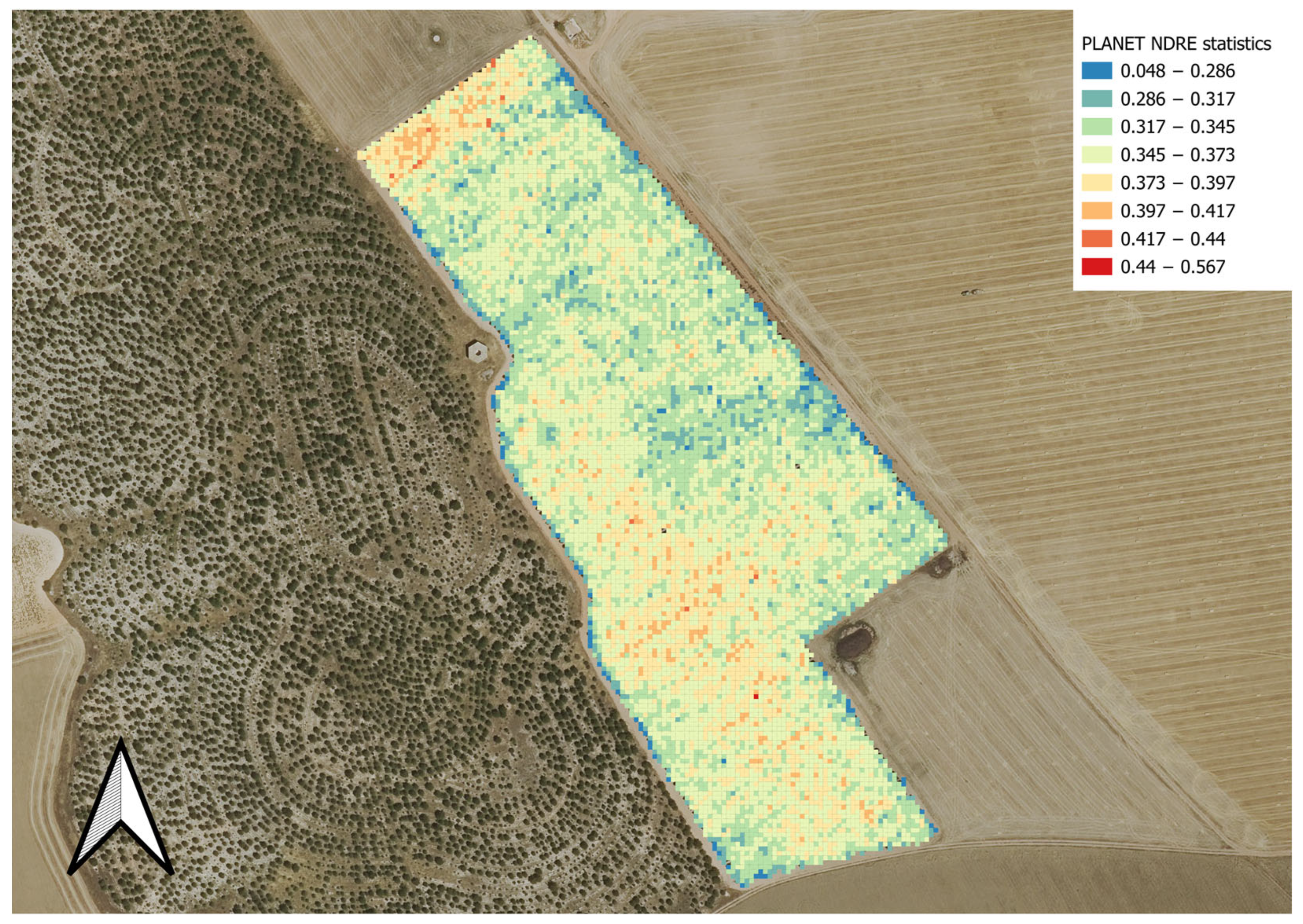
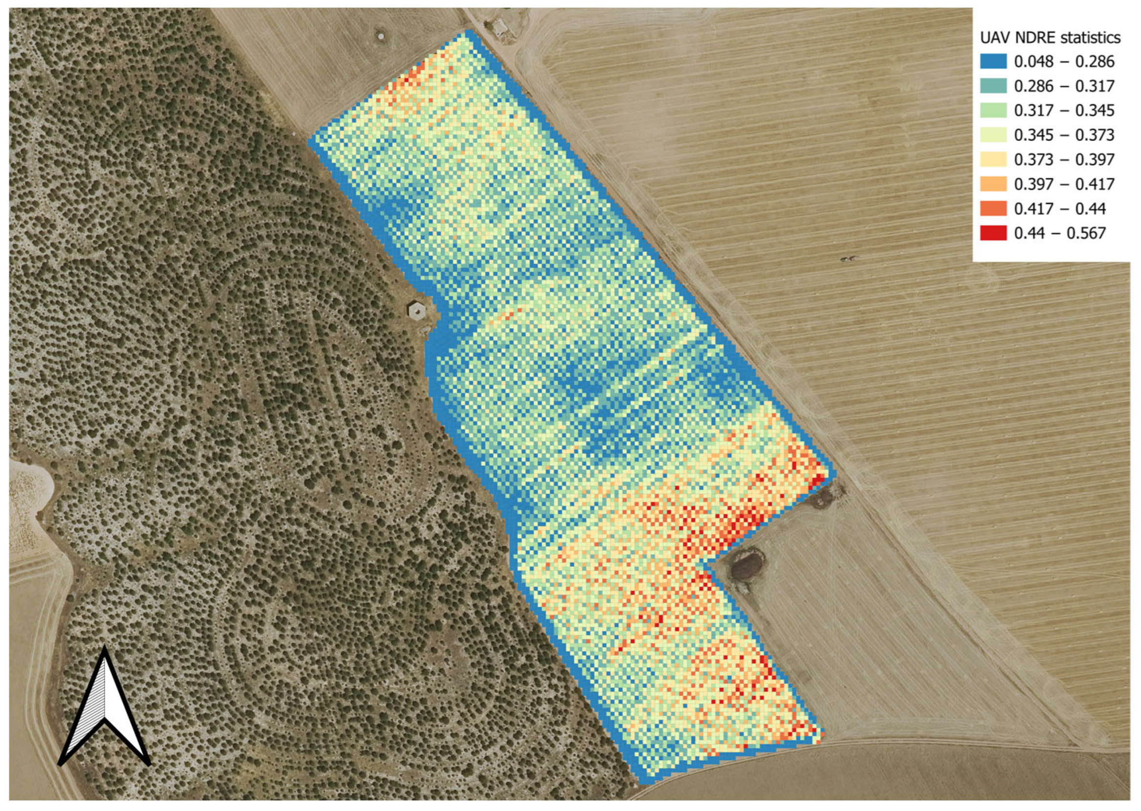
Figure 6 and Figure 7 illustrate the spatial distribution of the NDRE index for both sources. A common pattern emerges in the zoning, with higher vigour in the central areas of the crop and lower vigour observed at the edges. However, the UAV images provide a more accurate definition of tree lines and individual differences. This greater UAV accuracy enables farmers to detect intra-plot variability (i.e., differences between neighbouring trees), which satellites cannot distinguish. This is crucial for the early identification of water-, nutritional- or health-related stress problems. This pattern reflects the effects of microclimate and competition for resources: central trees typically have greater canopy density and water availability than peripheral trees, which are more exposed to environmental stress. In olive groves, where canopy variability can indicate soil limitation or management deficiencies, this finer resolution enables more precise adjustments to be made to irrigation or fertilization doses for specific areas, rather than applying uniform treatments across the entire farm.

3.2. Correlation Between Satellite Indices and UAVs

Spearman’s correlation was applied to the IVs to check whether both sources reflected the same spatial patterns.

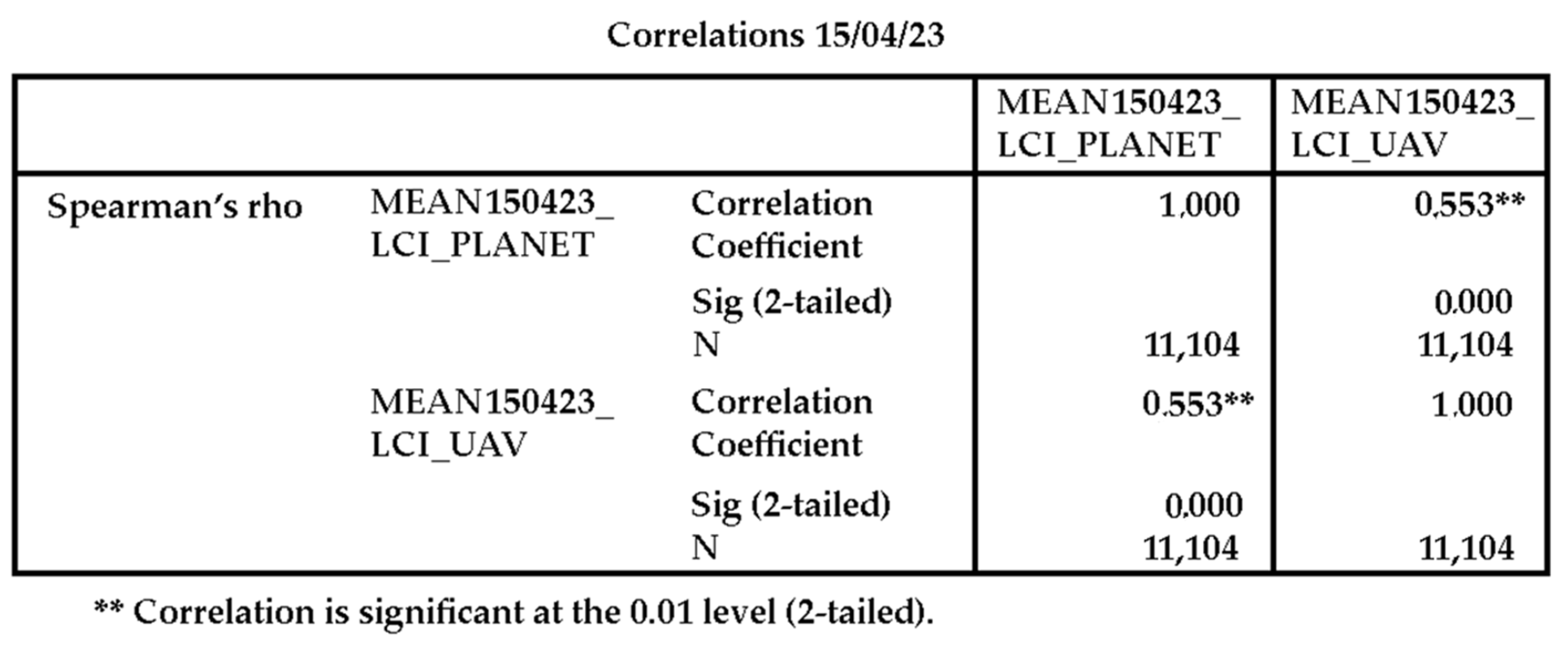
The results show a significant positive correlation (p < 0.001) in all cases (

Table 4. Spearman correlations, 290123.

29 January 2012	NDVI Planet	NDRE Planet	LCI Planet	GNDVI Planet
NDVI UAV	0.586	0.524	0.544	0.523
NDRE UAV	0.613	0.617	0.639	0.608
LCI UAV	0.604	0.608	0.625	0.597
GNDVI UAV	0	0.519	0.588	0.554

and

Table 5. Spearman correlations, 150423.

15 April 2023	NDVI Planet	NDRE Planet	LCI Planet	GNDVI Planet
NDVI UAV	0.543	0.976	0.998	0.939
NDRE UAV	0.89	0.538	0.529	0.479
LCI UAV	0.943	0.563	0.553	0.5
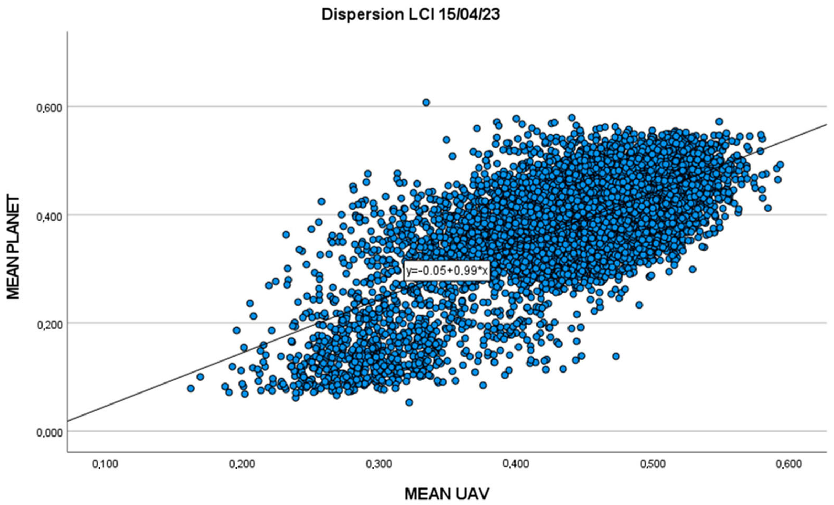
GNDVI UAV	0.903	0.547	0.536	0.544

), with correlation coefficients ranging from 0.45 to 0.68, depending on the IV and date. The LCI index presented the highest correlation (R = 0.625 in January and R = 0.553 in April), as shown in Figure 8 and Figure 9.

This indicates that, despite differences in resolution, both sensors detect similar patterns of vegetation vigour and can identify areas of overlap [71].

Although the absolute values differ, the existence of consistent correlations confirms that, while satellites are useful for general monitoring, UAVs offer added values for precise management, as they can distinguish minor canopy variations that are relevant to the final yield. The January stage (dormancy/pruning), which has lower vegetative activity and a more open canopy structure, showed higher correlations than April. This suggests that, during phases of low leaf cover, satellites can accurately represent general patterns. However, in April, when budding, flowering and leaf expansion occur, the structural complexity of the olive tree reduces satellites’ ability to capture actual variability. This finding is critical from an agronomic perspective, as April is a key stage in determining the future production load. This complementary evidence confirms the relevance of the chosen phases and demonstrates that the UAV–satellite correlation responds to critical agronomic changes in the olive tree cycle.

3.3. Statistical Comparison of Means

A Student’s t-test for related samples was performed to compare the mean values of each index between the two images for each individual (

Table 6. The results of the paired-samples Student’s t-test for image 290123.

Paired-Samples Test 29/01/23
		Pair Differences
					95% Confidence Interval of the Difference
		Mean	Std. Deviation	Std. Error Mean	Lower	Upper	t	df	Sig. (2-Tailed)
Pair 1	NDVI Planet-NDVI UAV	0.3435	0.0714	0.0007	−0.0357	−0.0330	−50.692	11,103	0.000
Pair 2	NDRE Planet-NDRE UAV	0.3334	0.6489	0.0006	−0.0396	−0.0372	−62.249	11,103	0.000
Pair 3	LCI Planet-LCI UAV	0.0550	0.0550	0.0005	0.0540	0.0560	105.273	11,103	0.000
Pair 4	GNDVI Planet-GNDVI UAV	0.0210	0.0412	0.0004	−0.0218	−0.0202	−53.661	11,103	0.000

).

A p-value of less than 0.001 was obtained; therefore, there were significant differences between the two sources for all variables evaluated on both dates. This confirms that sensors, although reflecting similar patterns, do not provide the same absolute values, with the UAV data being systematically higher due to its higher spectral and spatial resolution (

Table 7. The results of the paired-samples Student’s t-test for image 150423.

Paired-Samples t-Test 15/04/23
		Pair Differences
					95% Confidence Interval of the Difference
		Mean	Std. Deviation	Std. Error Mean	Lower	Upper	t	df	Sig. (2-Tailed)
Pair 1	NDVI Planet- NDVI UAV	0.0105	0.0816	0.0007	−0.0120	−0.0090	−13.56	11,103	<0.000
Pair 2	NDRE Planet- NDRE UAV	0.0764	0.0501	0.0005	−0.0773	−0.0754	−160.5	11,103	0.000
Pair 3	LCI Planet-LCI UAV	0.0586	0.0615	0.0006	0.0597	−0.0574	100.4	11,103	0.000
Pair 4	GNDVI Planet- GNDVI UAV	0.0452	0.0443	0.0004	0.0444	−0.0460	107.39	11,103	0.000

).

From a practical point of view, this difference means that UAVs can be used to calibrate satellite indices in olive groves with high precision. This enables local models to be scaled up to larger areas, thereby improving the transferability of results and facilitating the implementation of continuous monitoring programs.

3.4. Regression Models and Decision Trees

The possibility of predicting UAV sensor values from satellite data was explored. An attempt was made to fit a multiple linear regression model, using the NDRE values obtained from the UAV imagery as the dependent variable and the satellite values as the independent variables [80].

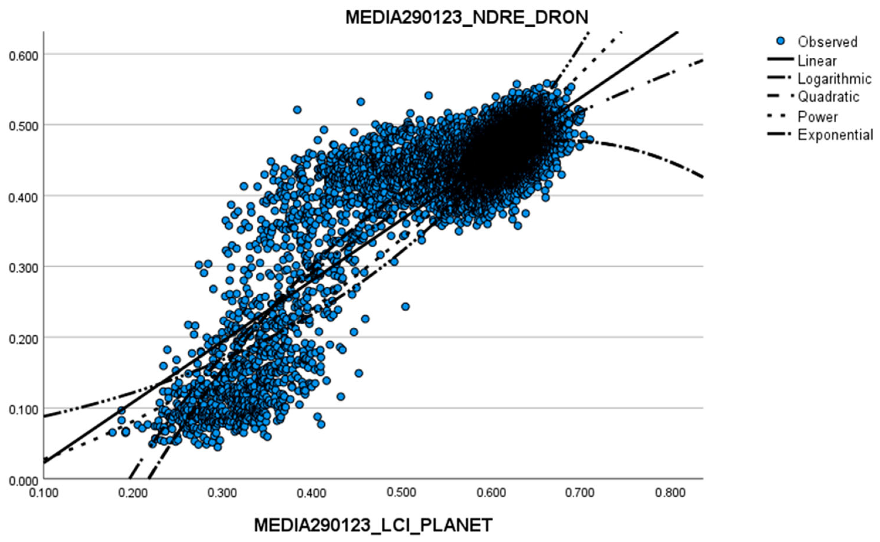
The independence of the satellite variables in relation to the drone’s dependent variable was analysed, along with the type of line that best fit each relationship. The example study for the dependent variable LCI is shown in

Table 8. Curvilinear estimation, NDRE/LCI 290123.

Model Summary and Parameter Estimates 29/01/23
Dependent Variable: NDRE DRON
Equation	Model Summary					Parameter Estimates
	R-Squared	F	df1	df2	Sig.	Constant	b1	b2	b3
Linear	0.753	33,823.186	1	11,102	0.000	−0.063	0.859
Logarithmic	0.788	41,331.599	1	11,102	0.000	0.664	0.407
Quadratic	0.805	22,909.451	2	11,101	0.000	−0.549	3.003
Cubic	0.805	22,909.451	2	11,101	0.000	−0.549	3.003	−2.2
Power	0.759	34,888.143	1	11,102	0.000	0.997	1.556	−2.2	0.000
Exponential	0.701	25,980.686	1	11,102	0.000	0.064	3.23

The independent variable is LCI Planet.

and Figure 10.

This study was carried out for all variables on both dates by creating the possible regression models and comparing the results. The null hypothesis (Ho) was that the variables could form a model because there was no significant relationship between them. Although all three options yielded a significance level of less than 0.05, indicating that a model could be formed with each (

Table 9. Regression models for Planet image 290123.

				Coefficients 29/01/23 a
		Unstandardized Coefficients		Standardized Coefficients			Correlations			Collinearity Statistics
Model		B	Std. Error	Beta	t	Sig	Zero. Order	Partial	Part	Tolerance	VIF
1	(Constant)	−0.063	0.003		−23.021	<0.001
	LCI Planet	0.859	0.005	0.868	183.911	<0.000	0.868	0.868	0.868	1.000	1.000
2	(Constant)	−0.194	0.009		−20.485	<0.001
	LCI Planet	0.585	0.020	0.591	29.935	<0.001	0.868	0.273	0.140	0.056	17.85
	GNDVI Planet	0.412	0.029	0.285	16.814	<0.001	0.859	0.135	0.067	0.056	17.85
3	(Constant)	−0.186	0.009		−19.566	<0.001
	LCI Planet	0.439	0.026	0.444	16.814	<0.001	0.868	0.158	0.078	0.031	32.075
	GNDVI Planet	0.304	0.031	0.210	9.72	<0.001	0.859	0.092	0.045	0.047	21.488
	NDVI Planet	0.22	0.026	0.224	8.389	<0.001	0.864	0.079	0.039	0.030	32.843

^a Dependent variable: MEDIA290123_NDRE_DRON.

), according to the collinearity diagnostics (

Table 10. Collinearity diagnostics.

			Collinearity Diagnostics 29/01/23 a
					Variance Proportions
Model	Dimension	Eigenvalue	Condition Index	(Constant)	LCI Planet	GNDVI Planet	NDVI Planet
1	1	1.988	1.000	0.01	0.01
	2	0.012	12.863	0.99	0.99
2	1	2.988	1.000	0.00	0.00	0.00
	2	0.012	15.740	0.09	0.05	0.00
	3	0.000	101.808	0.91	0.95	1.00
3	1	3.985	1.000	0.00	0.00	0.00	0.00
	2	0.014	16.937	0.09	0.01	0.00	0.00
	3	0.000	104.328	0.14	0.91	0.01	0.74
	4	0.000	121.915	0.77	0.08	0.99	0.26

^a Dependent variable: MEDIA290123_NDRE_DRON.

), only one of the models, NDRE_UAV = −0.063 + 0.859 × LCI_Planet (

Table 11. Summary of model 1.

		Model Summary 29/01/23 b
Model	R	R-Squared	Adjusted R-Squared	Std. Error of the Estimate	Durbin–Watson
1	0.896 a	0.803	0.803	0.0399706	1.001

^a Predictors (constant): LCI Planet, LCI PANET; ^b dependent variable: NDRE UAV.

), showed acceptable collinearity, with R² = 0.753. However, the Durbin–Watson statistic detected autocorrelation of residuals (DW = 0.974), so the linear model was discarded.

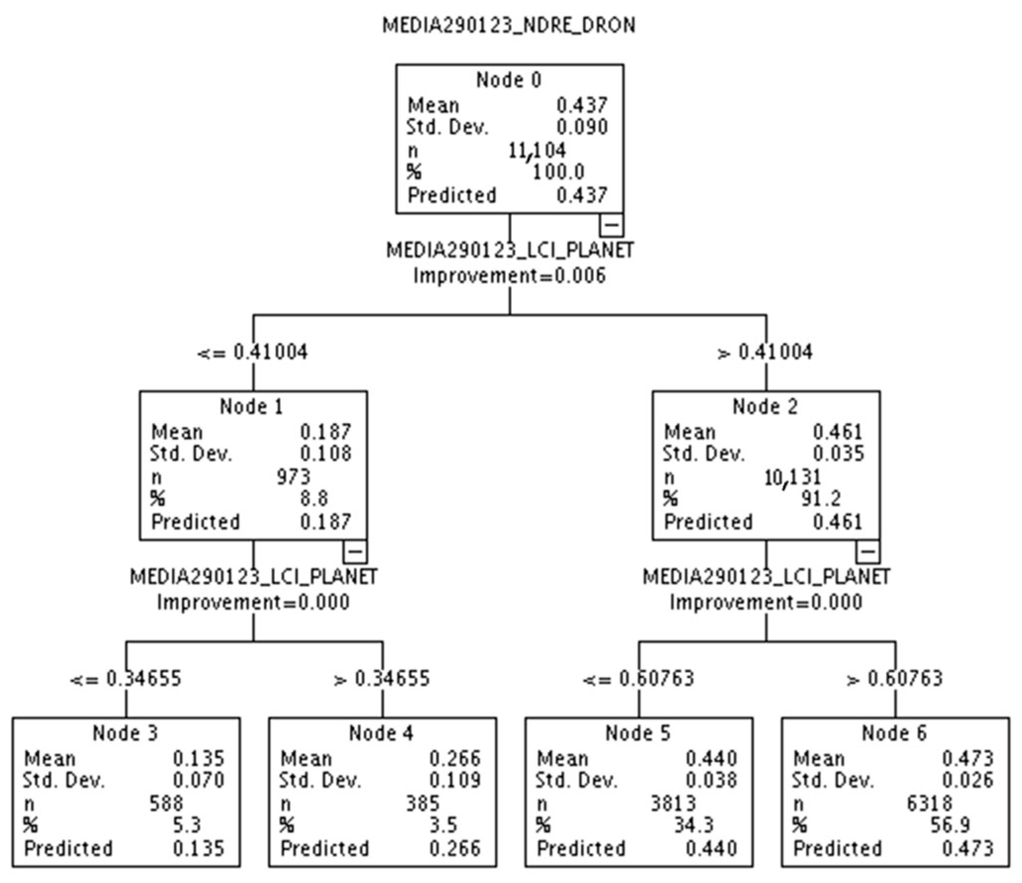
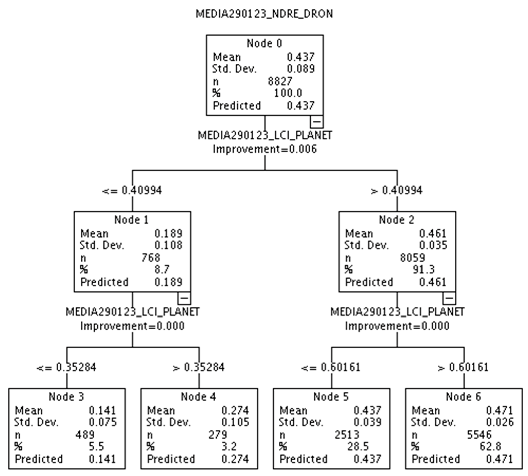
A non-parametric model based on decision trees Figure 11 was then chosen, which produced better results.

This model was tested by splitting it into test/sample groups, with the results shown in Figure 12 and Figure 13.

The root mean square error (RMSE) was 0.039 for the training set and 0.04 for the test set in January, remaining similarly low in April. A precision of more than 80% indicates good generalisability without signs of overfitting when non-parametric methodologies are applied in multi-source studies [71].

In decision trees, the satellite variables with the highest predictive power were NDRE and LCI. This is consistent with their sensitivity to photosynthetic activity and leaf chlorophyll content.

Compared to linear regression, decision trees achieved a 20–25% reduction in error. This demonstrates that this approach is more appropriate for perennial crops, such as olive trees, where the relationship between vigour, canopy structure and reflectance is nonlinear and influenced by multiple factors, such as canopy density, tree age and soil conditions.

This result shows farmers that UAVs do not always need to fly over the entire cropland: a satellite can provide baseline data and a decision tree can help identify areas where a UAV should be used to obtain more detailed information.

3.5. Crop Area Segmentation into Clusters

Finally, a two-stage hierarchical cluster classification was used for zoning the production area according to homogeneous management zones based on the individual IVs. Five- and ten-cluster classifications were compared for each date and sensor.

Classifying the results into 5 or 10 groups enabled a direct linkage to management practices. In 5-zone configurations, areas of high and low vigour can be identified to inform general fertilisation and irrigation strategies. In 10-zone configurations, greater discrimination enables more specific interventions to be designed, such as differential pruning or localised nutrient applications. This segmentation capability transforms the maps into operational tools for precision agriculture in olive groves.

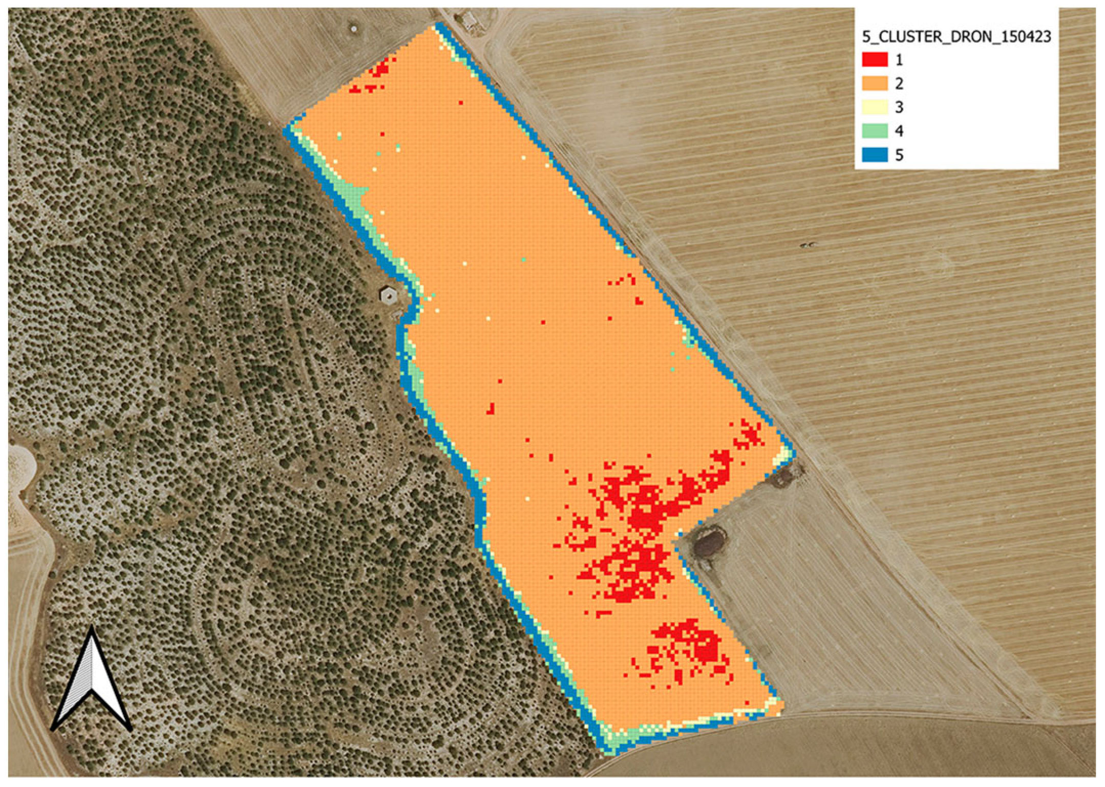
For the April drone data, five zones were identified (Figure 14 and

Table 12. Summary of the index values in each cluster in Planet image 150423 for 5 clusters.

Planet	Cluster	1	2	3	4	5
	SIZE	0.5% (61)	6.1% (680)	15.7% (1743)	9% (1001)	68.6% (7619)
	GNDVl	0.38	0.47	0.61	0.72	0.67
	LCI	0.09	0.16	0.33	0.51	0.41
	NDRE	0.08	0.14	0.27	0.42	0.34
	NDVI	0.36	0.42	0.51	0.6	0.59

), and the corresponding zone map is shown in Figure 15.

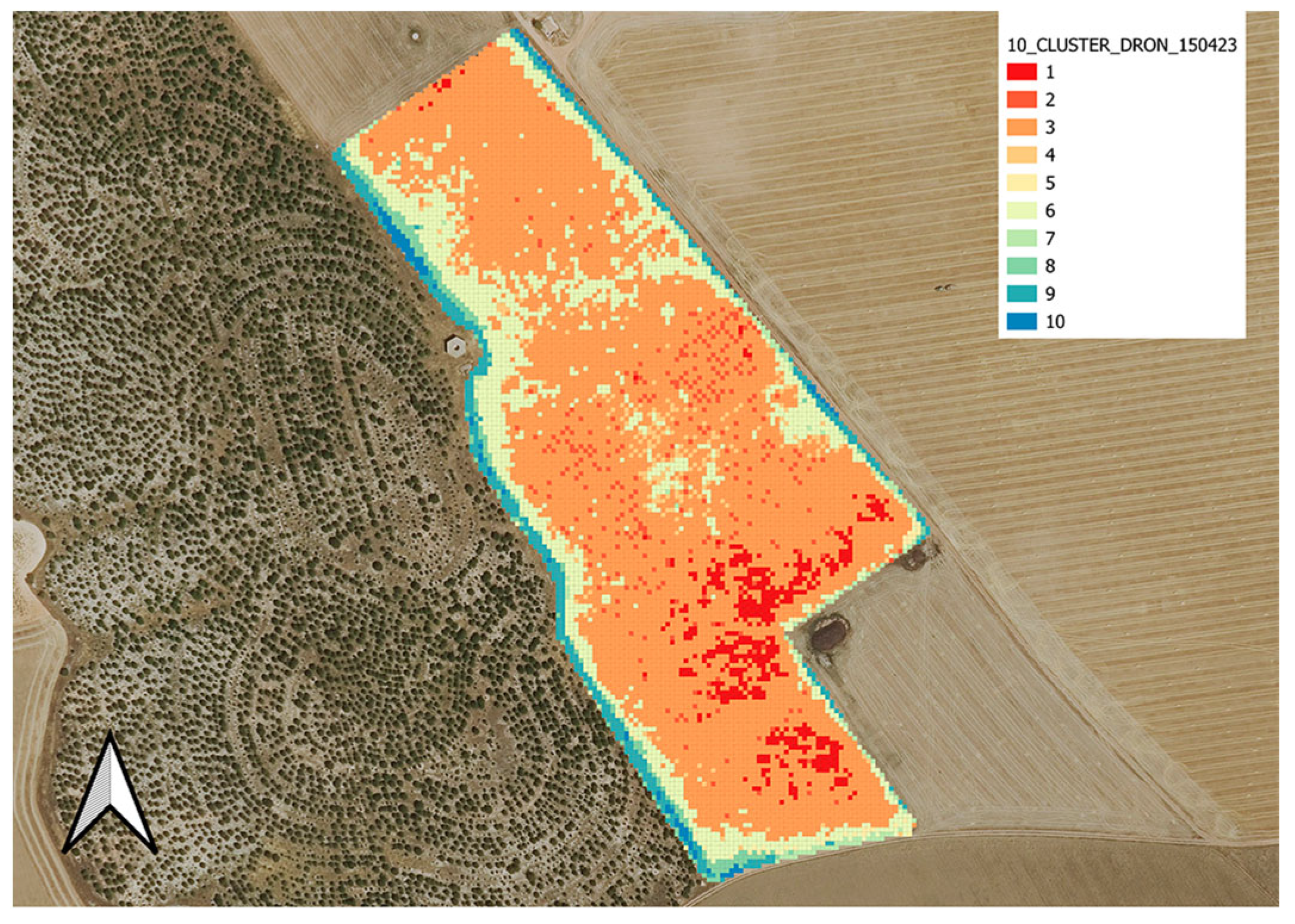
For the April drone data, ten zones were identified (Figure 16 and

Table 13. Summary of index values in each cluster for Planet image 150423 for ten clusters.

Planet	Cluster	1	2	3	4	5	6	7	8	9	10
	Size	0.2% (27)	3.7% (412)	1.3% (142)	2.4% (270)	7.2% (800)	2.3% (254)	3.6% (3994)	1.9% (214)	7.6% (849)	37.3% (4142)
	GNDVI	0.37	0.44	0.49	0.53	0.6	0.74	0.69	0.73	0.68	0.64
	LCI	0.09	0.12	0.2	0.22	0.32	0.53	0.45	0.52	0.42	0.37
	NDRE	0.08	0.11	0.17	0.18	0.27	0.43	0.37	0.42	0.35	0.31
	NDVI	0.34	0.4	0.52	0.41	0.49	0.64	0.61	0.55	0.51	0.57

), and the corresponding zone map is shown in Figure 17.

The same analyses were carried out on the Planet images on both dates, with the same results. Classifying the images into 10 clusters showed better discrimination, preventing outliers from being overly influential and providing a more detailed zoning.

The central zones of the crop, which exhibited higher vigour, could be clearly differentiated from the peripheral zones, which were more adversely affected by environmental conditions. This technique has been used successfully in similar studies on olive orchard intensification [76].

Cluster classification should be viewed as an agronomic zoning tool. In areas of greater vigour (central clusters), farmers can apply controlled deficit irrigation strategies to optimise water use without compromising production.

In peripheral areas, where vigour is low, this information enables informed decisions to be made regarding the provision of additional inputs (e.g., irrigation or fertiliser) or, in extreme cases, the implementation of management changes or replanting.

Thus, UAV and satellite-based zoning provide a direct route to precision agriculture in olive groves.

Overall, the results show that combining UAVs and satellites allows variability patterns to be captured and provides an objective basis for defining UAV activation thresholds. In other words, it enables anomalies that are significant enough to justify a drone campaign for a more detailed diagnostics to be identified when they are detected by the satellite.

4. Discussion

The comparative analysis of vegetation indices calculated from multispectral satellite and UAV images allowed us to evaluate the effectiveness of these technologies with respect to the monitoring of super-intensive olive orchards. This section discusses the study results in terms of data accuracy, correlation between images, and usefulness for decision making in agricultural management.

Although satellite images have a lower spatial resolution, this study has shown that they can capture general patterns of vigour in the crop, which is useful for obtaining a general overview of the state of the crop at a low operational cost. However, drone imagery can identify specific areas at the level of individual trees, which is essential for localised management applications such as differentiated fertilisation, disease detection or water stress damage assessment. Thess findings are consistent with those of Psomiadis et al. [71] and Bollas et al. [23], who reported correlation values above 90% between UAV and Sentinel-2 for the NDVI index. This reinforces our observation of a general correspondence between the two sources, although with higher definition in UAV imagery.

Significant correlations between sensors (the Spearman correlation coefficients ranged between 0.45 and 0.68, p < 0.001) indicate that, despite differences in scale and resolution, both systems record coherent spatial patterns. This level of agreement suggests that integrating both types of data is a viable approach for developing multiscale monitoring systems.

The fitted multiple linear regression model showed a high coefficient of determination (R² = 0.753) when the satellite-derived LCI was used to predict the UAV-based NDRE. However, due to autocorrelation in the residuals (DW = 0.974), this model was discarded in favour of a non-parametric solution. In this context, decision trees produced more accurate results, with low quadratic error (RMS = 0.004) and enabled robust prediction of UAV sensor values from satellite data without over-fitting.

This study further proposes the utilisation of the 10th percentile of the vegetation index values obtained by satellite as an activation threshold, with the objective of identifying critical areas. This threshold facilitates the identification of trees or areas exhibiting diminished vigour, thereby enabling the implementation of agronomic interventions (e.g., irrigation or diversified fertilisation) solely in instances where such intervention is genuinely imperative. The present approach has been shown to optimise resources and avoid including healthy areas, thereby maintaining precise and efficient intervention. This facilitates the planning of UAV flights with greater precision, enabling the inspection of trees that require intervention in a more targeted manner. This, in turn, optimises the allocation of time, financial resources and other assets. In this manner, the activation threshold provides a quantitative instrument for agronomic decision-making, whilst also ensuring the more efficient monitoring of intra-plot variability, stress and the growth of olive trees. This is in accordance with the objectives of precision agriculture.

These results are consistent with those of other studies that have integrated UAV and satellite data to predict crop response to varying nitrogen doses [81], demonstrating that non-parametric models can overcome the limitations of classical methods. Multisensor integration has also been identified as an effective approach for enhancing monitoring accuracy without losing scalability [23,79].

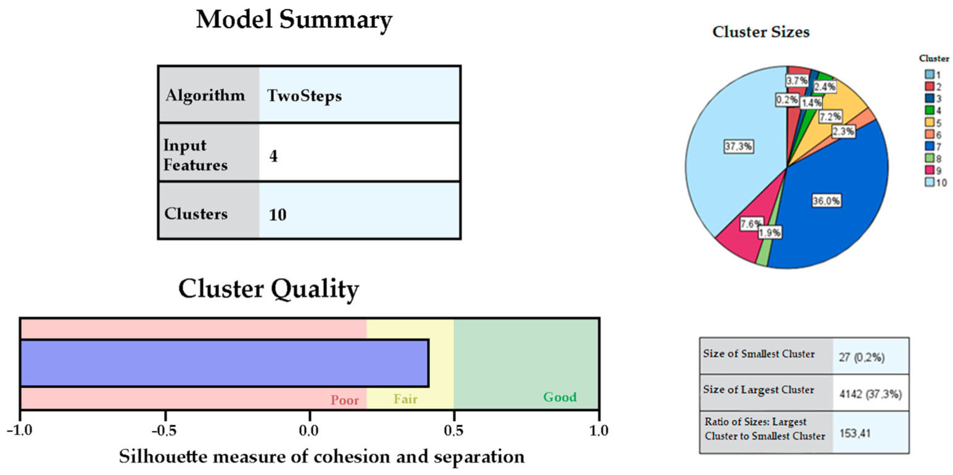
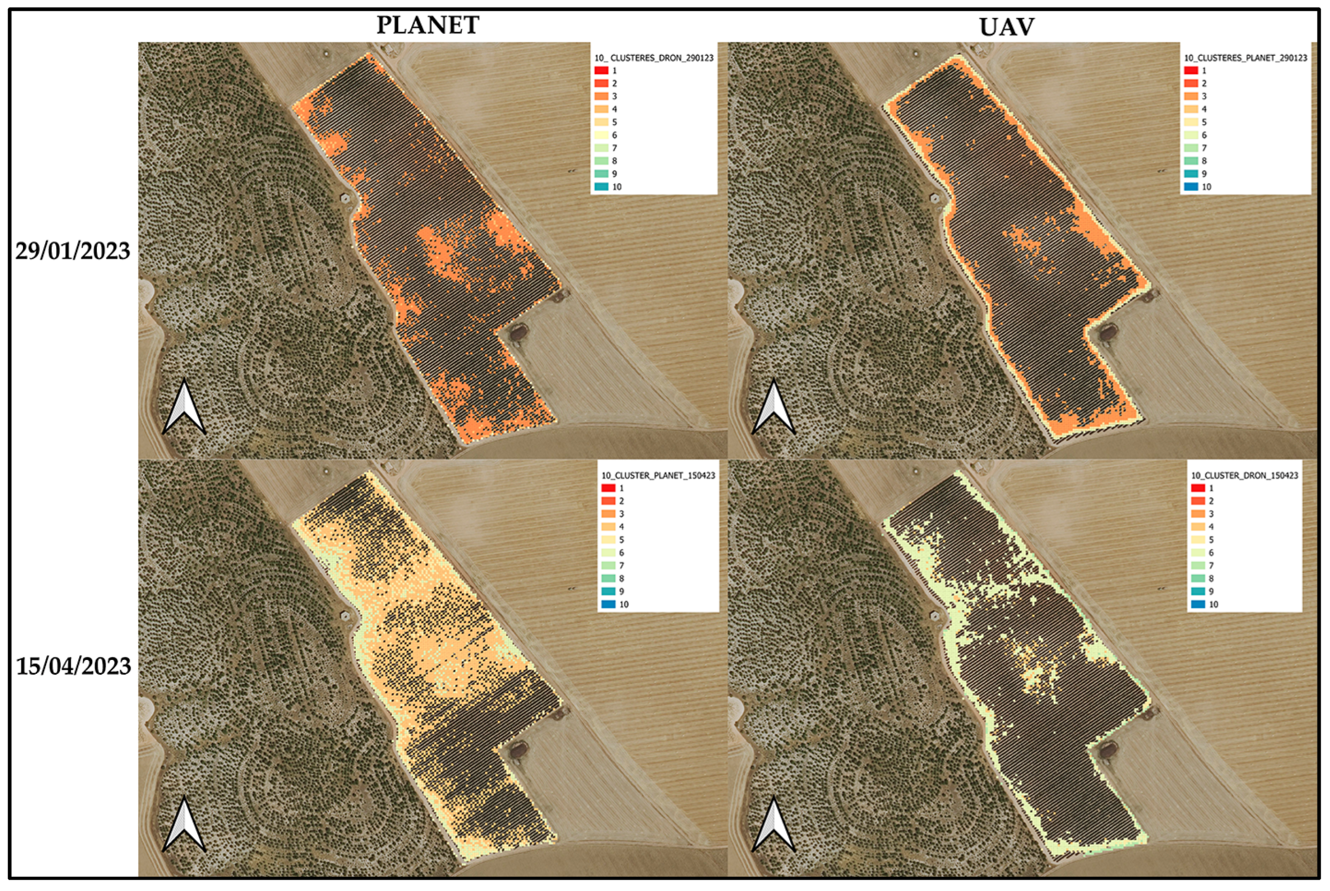
Cluster segmentation was also a key component of the analysis, as it enabled the crop to be divided into homogeneous management zones according to the spectral behaviour of the trees. The 10-cluster classification was more efficient than the 5-cluster classification, as it avoided the overlap of extreme values and showed better differentiation of intermediate zones, which could be missed in a more general zoning system (Figure 18). The selection of the optimal number of clusters (k) was based on a combined evaluation of agronomic coherence and statistical consistency criteria. A comparative analysis was conducted on solutions exhibiting varying k values (ranging from 5 to 15). It was observed that a stabilisation point was attained in the reduction of intragroup variance around k = 10. This finding suggests that increasing the number of groups does not result in a significant enhancement of internal differentiation. This behaviour, analogous to that observed using the elbow method, was utilised as a reference to define the final structure of the classification. Moreover, this solution offered optimal spatial correspondence between dates, thereby circumventing overlaps of extreme values and enabling the agronomic interpretation of homogeneous management areas [28,29,82,83].

For the April case study of Planet, it was observed that the difference in cohesion measures between five and ten zones is very similar (0.4). However, the size of the groups was, for five clusters, 7619 individuals, i.e., 68.6% of the cases, generating poor zoning due to the existence of extreme values that needed to be considered. Analysing the zoning in ten clusters resulted in a better distribution of the data, with the largest group size being 4142 individuals, corresponding to 37.3%. It was therefore decided to use the 10-cluster classifications.

For the January images, the olive tree canopies were relatively homogeneous, which was reflected by both sensors, clearly showing the zones segmented by clusters. However, in the April images, a greater variability in the condition of the olive trees was observed, coinciding with the phenological stage of the crop during which buds appear that will later develop into flowers or new shoots. In this case, although the areas identified were the same for both sensors, the drone showed a higher resolution, which made it possible to locate the problem areas with greater precision, as shown in Figure 19.

The ability to identify variations within plots at pivotal stages of the growth cycle is crucial for predicting variations in growth, vigour and productivity between neighbouring trees. This has direct implications for planning irrigation and fertilisation.

This zoning can be applied directly to precision agricultural management strategies, such as irrigation planning, fertilisation and sampling. In this way, maps derived from remote sensing serve as visual representations and decision-support tools, enabling the optimisation of inputs, reduction of costs and improvement of sustainability. Segmentation based on multispectral indices is a useful tool for data-driven agronomic planning, as highlighted in articles on technological innovation in olive growing [77].

Despite the large number of studies examining the integration of remote sensing in precision agriculture [84,85,86], few focus specifically on super-intensive olive orchards. This work is novel in that it compares UAV and satellite imagery in real conditions, employs detailed statistical and spatial analyses and proposes predictive models with practical implications. Specifically, two predictive approaches were evaluated: a multiple linear regression model (NDRE_UAV = −0.063 + 0.859 × LCI_Planet), which achieved a high coefficient of determination (R² = 0.753) but was discarded due to autocorrelation in the residuals (DW = 0.97); and a non-parametric model based on decision trees, which offered better performance (RMSE = 0.04, accuracy > 80%) and higher generalisability. The fact that decision trees proved more appropriate is explained by their ability to handle nonlinear relationships and physiological response thresholds that are common in woody crops, where growth and production do not increase proportionately to inputs (water, nutrients), but rather present saturation points or differential responses depending on the phenological stage.

Progress has been made compared to previous work, as it includes spatial clustering techniques applied at the individual (tree) scale, instead of homogeneous blocks or grids. It also provides a methodological improvement by applying a robust statistical validation, including hierarchical geospatial segmentation and focusing on highly specific woody crops such as super-intensive olive groves, which have received little attention the literature. This approach differs from previous work, in which instance segmentation was applied using convolutional neural networks to estimate individual canopy biometry in traditional olive orchards based on geometric variables [27]. However, the approach of this study combines segmentation scale with multispectral analysis, UAV/satellite correlation and predictive modelling to generate management zones.

A comparison of this study with recent research in this field [87,88] indicates that it underlines the potential of machine learning models applied to agricultural remote sensing. However, the present study focuses on the adaptation of these models to woody crops and the segmentation of these crops at the individual level.

This study complements and extends the approaches developed for annual crops such as maize, wheat and onions [23,79,81] by transferring these methodologies to the context of woody crops, whose physiological responses and management present different particularities. Compared to other perennial crops, such as vines and stone fruit trees, olive trees respond more slowly to interventions. At the same time, they are highly sensitive during phases such as budding and flowering in April, when water or nutritional stress can have a decisive impact on production in the following season [14,89]. These findings improve the methodological basis for multiscale monitoring of olive orchards, proposing a scalable, validated and adaptable integration methodology that contributes to the development of intelligent decision support systems for the agricultural sector.

Finally, this study has several limitations that require further discussion. The spatial representativeness of UAVs may be restricted by the size of the plots and the partial coverage of the flights, limiting the ability to generalise results to regional scales.

The comparison between UAVs and satellites is affected by inherent differences in spatial and spectral resolution, which can amplify or reduce the detected differences. Furthermore, the temporal extrapolation of the results is limited to two phenological stages (winter and spring), meaning that critical stages of the olive tree, such as fruit enlargement and ripening, are not covered.

Furthermore, the availability of UAV data and its operational cost continue to hinder the scalability of these methods in larger production systems, where satellites are more accessible. As pointed out multiscale integration requires statistical tools, as well as calibration and cross-validation protocols, to ensure consistency between data sources.

Recognising these limitations does not undermine the findings; rather, it defines the scope of application and suggests future areas of research, such as incorporating longer time series, exploring the use of hyperspectral and thermal sensors, validating the results in other olive-growing regions and comparing the approach with other woody crops, such as grapes, almonds and citrus fruits. This will enable an evaluation of the robustness and transferability of the approach.

5. Conclusions

This study confirms the effectiveness of the combined use of multispectral images acquired by satellites and UAVs for detailed monitoring of olive crops. By comparing vegetation indices such as NDVI, NDRE, LCI and GNDVI, this work shows that UAV images provide a higher level of resolution and precision, allowing the detection of specific problems at the plant level. However, satellite images, despite their lower resolution, facilitate the analysis of spatial variability patterns at a larger scale and with more continuous temporal coverage.

The results of this study show that satellite images are particularly useful for providing an overview of the crop and identifying areas of interest for monitoring. On the other hand, UAV images allow detailed zoning, improving accuracy in the classification of specific management areas within the olive grove, optimising input management and facilitating a form of precision agriculture that is more adapted to the requirements of each crop. In the analyses carried out, a significant correlation was observed between the vegetation indices obtained with both technologies. Moreover, the use of statistical methods such as Spearman’s correlation coefficient and multiple regression showed that both types of images exhibited similar patterns of vigour and crop stress, with statistically significant results (p < 0.001), particularly evident in the LCI index.

Furthermore, the non-parametric models based on decision trees outperformed linear regressions in terms of error and generalisability, achieving an RMSE of 0.04 and an accuracy of over 80%. This reinforces the usefulness of flexible approaches in complex agricultural scenarios.

This study, however, has limitations. The need to match the resolution between satellite and UAV images using a 3 × 3 m mask may introduce errors due to the averaging of multi-pixel values in the UAV imagery. This suggests that, for future studies, multitemporal data should be integrated throughout the whole phenological cycle of the olive tree, along with field validation using physiological or yield variables. It would also be useful to incorporate methods based on object-oriented analysis to improve the discrimination between vegetation and soil.

In light of the results obtained, a hybrid approach is recommended, combining the wide coverage of satellite images for the initial detection of variations, followed by the detailed analysis of UAVs in specific areas. This approach not only optimises costs by reducing the frequency of UAV flights but also improves the ability to respond to specific crop problems, such as water stress or pest detection. In addition, to improve monitoring efficiency and accuracy, future research should explore the use of advanced data fusion technologies and the integration of other sensors, such as hyperspectral or thermal sensors, to provide additional information on crop health and vigour.

This work adds to the limited but growing literature on precision olive growing, especially in super-intensive systems. This research provides results that are applicable to a permanent woody system.

In conclusion, this study demonstrates the potential of the combined use of remote sensing technologies in precision agriculture, providing a replicable and scalable tool for woody crops with uniform structure. The integration of multispectral imagery and advanced analysis techniques reinforces the importance of these approaches in optimising resource use, improving productivity and promoting more sustainable agricultural management.

This study demonstrates that the combination of UAV and satellite multispectral data is an effective strategy for agronomic monitoring of super-intensive olive orchards. The integration of these makes it possible to take advantage of the strengths of each: on the one hand, the high spatial resolution of UAV enables the identification of variability at the individual tree level; on the other hand, satellite images offer a higher temporal resolution frequency and wider coverage, facilitating more consistent and cost-effective operational monitoring.