Phenology-Based Maize and Soybean Yield Potential Prediction Using Machine Learning and Sentinel-2 Imagery Time-Series

Featured Application

Crop yield potential prediction based on phenological modeling from remote sensing data and machine learning can provide a low-cost alternative to yield mapping sensors on combine harvesters for determining yield productivity zones for precision agriculture.

Abstract

Unlike traditional yield mapping, which is conducted using costly yield sensors mounted on combine harvesters to collect post-harvest data, yield potential prediction using remote sensing data is considered a low-cost alternative. In this study, an effort was made to address the research gap concerning the effectiveness of phenological modeling in crop yield potential prediction using machine learning. Combinations of seven vegetation indices from Sentinel-2 imagery and seven phenology metrics were evaluated for the prediction of maize and soybean yield potential. Ground truth yield data were provided by the Quantile Loss Domain Adversarial Neural Network (QDANN) database, with 1000 samples randomly selected per year from 2019 to 2022 for Iowa and Illinois. Four machine learning algorithms were tested: random forest (RF), support vector machine regression (SVM), multivariate adaptive regression splines (MARS), and Bayesian regularized neural networks (BRNNs). Across all evaluations, RF was found to outperform the other models in both cross-validation and final model accuracy metrics. Vegetation index values at peak of season (POS) and phenological timing, expressed as the day of year (DOY) of phenological events, were identified as the most influential covariates for predicting yield potential in particular years for both maize and soybean.

1. Introduction

Conventional crop yield estimation relies heavily on field surveys, manual sampling, and agrometeorological models, which are often labor-intensive, time-consuming, and prone to human error [1]. Traditional methods involve collecting data from representative plots through destructive sampling, where crops are harvested and weighed to extrapolate yield for larger areas [2]. Additionally, empirical models based on historical yield data, weather parameters, and soil conditions are used to predict productivity [3]. While these approaches have been the backbone of agricultural planning and policymaking, they suffer from several limitations, including spatial inconsistency, delayed reporting, and high operational costs [4]. Moreover, such methods lack real-time monitoring capabilities, making them less responsive to sudden environmental stressors, such as droughts, pests, or diseases [5]. These inefficiencies can lead to inaccurate yield forecasts, affecting food security assessments, market pricing, and resource allocation. Given the increasing global population and climate variability, precise and timely yield potential prediction is critical for ensuring sustainable agricultural productivity [6]. Transitioning from conventional to data-driven approaches can enhance accuracy, reduce costs, and support proactive decision-making in agriculture [7]. Thus, improving yield potential prediction methodologies is not only essential for optimizing farm management but also for strengthening food supply chains and mitigating economic risks in the face of growing climatic uncertainties [8]. Unlike traditional yield mapping, which relies on expensive yield sensors mounted on combine harvesters to collect post-harvest data [9], yield potential prediction based on remote sensing data provides a potential low-cost alternative for optimizing crop production in forthcoming years. By identifying underperforming fields early, precision agriculture strategies can be implemented to narrow yield gaps, leading to more sustainable production [10]. As climate change introduces greater unpredictability in growing conditions, early and accurate yield potential estimation becomes even more critical [11]. By shifting from reactive yield mapping to predictive analytics, agriculture can transition toward data-driven, climate-resilient farming, ensuring stable production in the coming decades [12]. This approach not only improves farm-level profitability but also contributes to global food security by reducing waste and optimizing land use efficiency [13]. Notably, maize and soybean are globally vital crops [14,15], serving as key sources of food, feed, and biofuel, while their symbiotic nitrogen fixation and high productivity contribute significantly to agricultural sustainability and food security.

Since traditional yield estimation methods, including field surveys and agrometeorological models, are often limited by spatial and temporal scalability, as well as high costs, remote sensing was increasingly researched to help overcome these obstacles [16]. In particular, multispectral satellite missions, like Sentinel-2, offer a transformative alternative by enabling continuous, non-destructive monitoring of crop health and growth dynamics [17,18]. Among the most applicable data for crop yield potential prediction derived from satellite data are vegetation indices and phenology metrics, which provide key insights into plant biophysical parameters and developmental stages, thereby enhancing yield prediction models [19]. Vegetation indices based on multispectral imagery, among which the normalized difference vegetation index (NDVI) and enhanced vegetation index (EVI) are most frequently used in previous research [20,21,22], provide high correlations with crop vigor, biomass, and photosynthetic activity. These indices exploit the reflectance properties of vegetation in the red and near-infrared spectral bands, allowing for the quantification of chlorophyll content and canopy structure [23]. Sentinel-2’s relatively high temporal (5 days at the equator) and spectral resolution (13 spectral bands) make it particularly suitable for tracking subtle changes in crop conditions throughout the growing season [24]. Time-series vegetation index data have been widely used in previous studies, providing a potential way to improve crop yield potential prediction accuracy compared to traditional methods [25]. However, yield forecasting can be further refined by incorporating phenology metrics, which capture the timing and duration of key crop growth stages [26]. Phenology modeling utilizes remote sensing to identify critical transition points in the growing cycle, such as the start of season (SOS), peak of season (POS), and end of season (EOS), which are influenced by climatic conditions, soil properties, and agronomic practices in the field [27]. With the relatively high temporal resolution of the Sentinel-2 satellite mission allowing for the calculation of dense phenological curves, the detection of anomalies, such as delayed emergence or premature senescence due to drought or disease, is enabled [28]. These metrics can be integrated into machine learning regression models to improve relationships between phenological dynamics and crop yield potential but the present state of research on the topic is scarce. Recent studies, such as Amankulova et al. [29], Sharifi [30], and Desloires et al. [31], have shown that combining phenological features with machine learning improves yield prediction accuracy across crops and environments, especially when using time-sensitive indices during flowering or grain-filling stages. Specifically, Desloires et al. [31] demonstrated significant performance gains in maize yield forecasting when using phenology-based vegetation features, which were focused on growing degree day-based modeling. Similarly, Joshi et al. [32] and Shuai et al. [33] emphasized that integrating dynamic indicators like phenology stages into machine learning enhances spatial and temporal generalizability compared to using aggregated indices alone. Despite these advancements, neither study considered a comprehensive combination of several vegetation indices and phenology metrics, particularly under varied climatic and management regimes.

The integration of machine learning into agriculture has notably improved traditional farming practices by enabling data-driven decision-making, improving resource efficiency, and enhancing crop productivity [34,35,36]. One of the most promising applications of machine learning is crop yield potential prediction, which utilizes computational algorithms to analyze complex agricultural datasets and forecast yields with high accuracy [37]. By processing big data derived from multispectral satellite imagery, machine learning models can uncover non-linear relationships that cannot be detected using conventional statistical methods, thereby optimizing agricultural management and reducing uncertainty in yield potential prediction [38]. A key advantage of machine learning in agriculture is its ability to integrate multiple combinations of vegetation indices and phenology metrics, which are critical for assessing crop health and growth stages [39]. Vegetation indices serve as proxies for chlorophyll content, biomass, and photosynthetic activity, while phenology metrics capture the timing of key growth stages [28]. Machine learning algorithms based on a wide range of prediction approaches, including decision trees, support vector machines and neural networks, can process these temporal and spatial datasets to identify yield-influencing covariates [40]. By training models on historical yield data alongside real-time remote sensing inputs, machine learning systems can predict yield potential at field, regional, or global scales, accounting for variability in soil types, microclimates, and farming practices [41]. The fusion of machine learning with time-series phenology modeling allows for dynamic yield adjustments as the growing season progresses, updating yield potential prediction insights before harvest [42].

Due to the aforementioned research gap and lack of knowledge on the effectiveness of phenological modeling in crop yield potential prediction using machine learning, the aim of this study was to evaluate the combinations of seven vegetation indices from Sentinel-2 images and seven phenology metrics for the yield potential prediction of maize and soybean. This approach also provided evaluation of frequently used machine learning algorithms for yield potential prediction and additional observations on crucial phenological stages in that prediction, providing guidance for future studies.

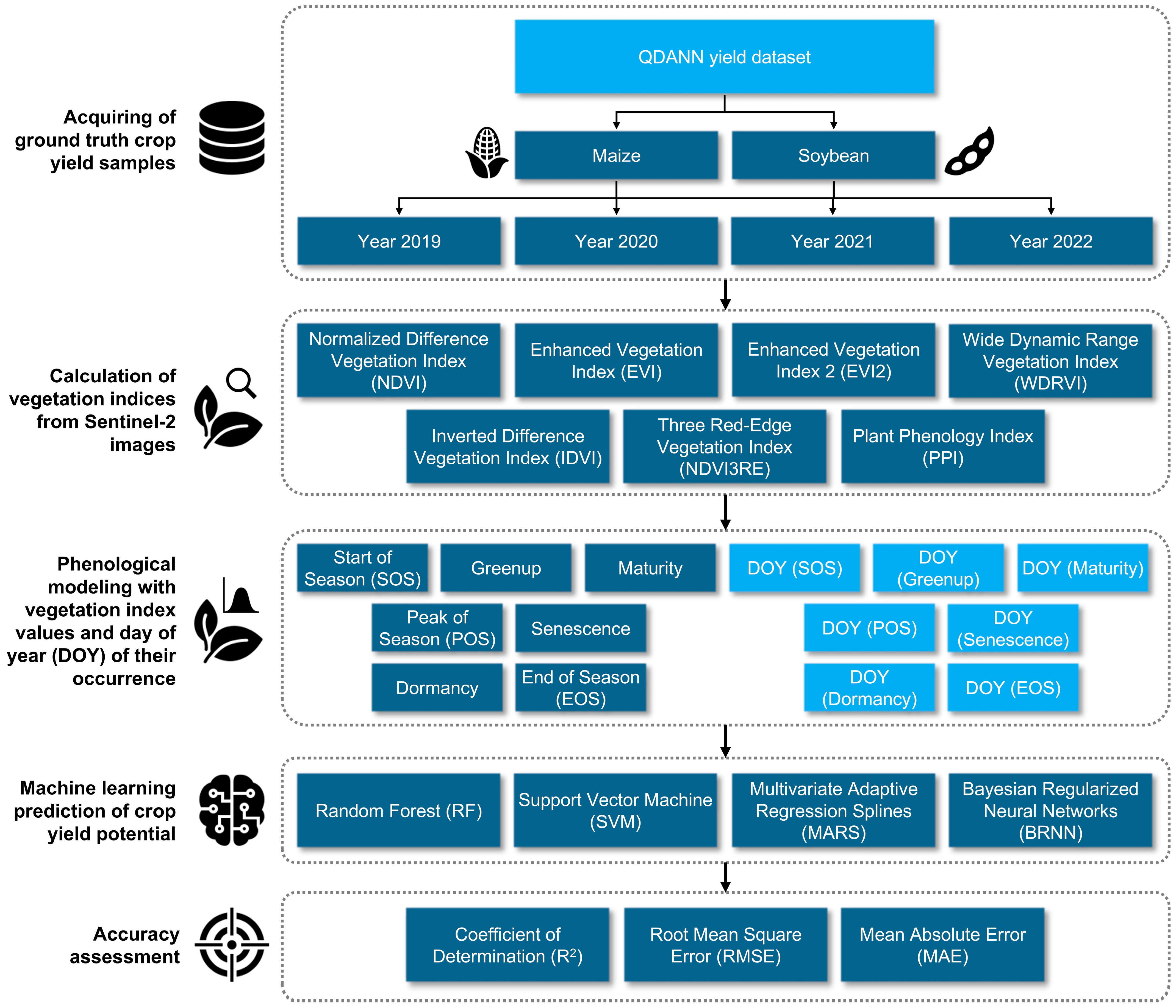
2. Materials and Methods

The workflow of the used methodology for crop yield potential prediction using machine learning, which was based on phenological modeling using vegetation indices from Sentinel-2 images, consisted of five fundamental steps: (1) acquiring of ground truth crop yield samples in a four-year study period (2019–2022); (2) calculating seven vegetation indices from Sentinel-2 images per sample, with a focus on evaluating novel saturation-resistant indices; (3) phenological modeling based on all seven evaluated vegetation indices; (4) predicting crop yield potential for maize and soybean with machine learning; and (5) assessing the accuracy of the predicted crop yield potential (Figure 1).

2.1. Study Area and Crop Yield Data

The study area included two major agricultural states, Iowa and Illinois, that are key contributors to United States maize and soybean production [43]. These states lie within the Corn Belt, a region known for its fertile soils with high organic matter and nitrogen content [44]. The climate across the study area is classified as a humid continental type (“Dfa” per Köppen climate classification), characterized by warm summers and significant seasonal precipitation variability [45]. The high-resolution maize and soybean yield data was obtained from the Quantile Loss Domain Adversarial Neural Network (QDANN) database, which included 30 m resolution yield maps for maize and soybean by integrating county-level yield statistics with remote sensing inputs [46]. This approach mitigated the scarcity of ground truth yield data while maintaining subfield spatial accuracy. However, while the QDANN dataset was developed using comprehensive ground truth crop yield datasets from yield mapping systems from combine harvesters, it results from statistical modeling and thus contains a bias [46]. The time frame of the research included a subsequent four-year period from 2019 to 2022, which represents the most recent available data in the QDANN dataset. For model training and testing, a total of 1000 randomly distributed sample points per crop annually was generated from the QDANN database to capture spatial heterogeneity in soil, climate, and management conditions (Figure 2). The sampling grids were adjusted each year to reflect crop rotation patterns, thereby preventing repetitive sampling of the same fields and increasing interannual variability in environmental conditions and management practices. A spatial autocorrelation test of the input crop yield values per dataset was performed using Moran’s I.

2.2. Calculation of Vegetation Indices from Sentinel-2 Images

The study utilized Sentinel-2 Level-2A bottom-of-atmosphere (BOA) surface reflectance images acquired between 2019 and 2022 [24]. These multispectral images were preprocessed through the Google Earth Engine platform [47], which enabled efficient handling of large geospatial datasets across the four-year study period. The Level-2A products provided atmospherically corrected surface reflectance values with an initial spatial resolution ranging up to 10 m depending on the spectral band [24]. To achieve the same spatial resolution as the input crop yield data from QDANN, all bands were resampled to a 30 m resolution using the bilinear interpolation method. Both crop yield values and surface reflectance time-series values from Sentinel-2 were obtained based on raster–vector overlay from the preprocessed data. The cloud masking procedure employed a multi-layered approach combining the scene classification layer (SCL) with probabilistic cloud and snow masks. Pixels were retained for analysis only when meeting all of the following criteria: a cloud probability below 5% (MSK_CLDPRB), the absence of cirrus clouds (SCL ≠ 10), and no cloud shadow effects (SCL ≠ 3).

Seven vegetation indices were calculated from the processed Sentinel-2 imagery. For each sample point, a complete time-series was generated by aggregating all available cloud-free observations within each study year. The temporal density of observations varied depending on cloud cover conditions but typically included 35–40 total scenes per study year. The extraction process automatically flagged and removed invalid values and eliminated duplicate observations that might occur when multiple scenes covered the same location within a short timeframe. The selected vegetation indices represented a combination of established metrics and innovative approaches designed to address the saturation effect in crop monitoring [26]. The NDVI [48] was included as a baseline reference due to its widespread use in agricultural remote sensing, despite its recognized saturation effects in dense canopies. Additionally, the EVI [49] was included, which introduces a soil adjustment factor and atmospheric resistance through inclusion of the blue band. The two-band EVI2 [50] was also included, as it maintains similar advantages to EVI while eliminating dependence on the blue band, making it compatible with a wider range of sensors. Besides these well-known indices, the wide dynamic range vegetation index (WDRVI) [51] incorporated a weighting coefficient to the near-infrared band, effectively extending the dynamic range and reducing saturation effects in high-biomass conditions. The inverted difference vegetation index (IDVI) [52] was implemented as a linear alternative to the NDVI, emphasizing absolute NIR reflectance rather than normalized ratios to maintain sensitivity across all growth stages. The three red-edge vegetation index (NDVI3RE) [53] utilized three of Sentinel-2’s red-edge bands to enhance discrimination in crops with a high leaf area index, where traditional NDVI underperforms. Finally, the plant phenology index (PPI) [54] was included specifically for its ability to track photosynthetic activity and vegetation phenology through unique band combinations.

2.3. Phenological Modeling Based on Vegetation Indices from Sentinel-2 Images

The extraction of phenological metrics from vegetation index time-series data was conducted using the phenofit package [55] in R v4.5.0 [56], which integrated curve fitting, smoothing, and quality assessment of seasonal dynamics. This analysis was performed at the individual yield sample point level, with each sample processed independently to account for spatial variability in crop growth patterns. For each vegetation index, a separate phenological curve was fitted to ensure comprehensive characterization of crop development stages. The Beck logistic model was selected as the primary curve-fitting algorithm due to its demonstrated effectiveness in smoothing noise inherent in remote sensing data while accurately capturing critical phenological transitions [57]. The curve-fitting process involved optimizing model parameters to best represent the observed VI temporal patterns while maintaining biological validity [58]. Curve fit diagnostics were performed using the coefficient of determination, the Nash–Sutcliffe model efficiency coefficient, and the observed and simulated coefficients of variation, which were used for the weighting of vegetation indices during the calculation of transition dates [59]. Seven key phenological transition dates were derived from the fitted curves, following established protocols in vegetation phenology research: start of season (SOS), greenup, maturity, peak of season (POS), senescence, dormancy and end of season (EOS). Each transition point was defined based on specific characteristics of the fitted logistic curve and its ecological significance in crop growth cycles, as explained in [26]. For each derived phenological metric, both the day of year (DOY) and corresponding vegetation index value were retained as covariates for yield potential prediction. This dual representation allowed for the investigation of both temporal (growth stage timing) and physiological (vegetation status at key stages) influences on crop productivity.

2.4. Machine Learning Prediction of Crop Yield Potential

Four machine learning algorithms were evaluated for the prediction of crop yield potential, including random forest (RF), support vector machine regression (SVM), multivariate adaptive regression splines (MARS), and Bayesian regularized neural networks (BRNNs). These algorithms were selected due to their high prediction accuracy in similar studies [60,61,62], as well as for their unique capabilities in handling complex, nonlinear relationships between crop yield and covariates from the vegetation indices and phenology metrics. The implementation followed a standardized workflow, which included standardization and outlier removal using the interquartile (IQR) approach as data preprocessing, model training, hyperparameter optimization, variable importance calculations, and accuracy assessment. All combinations of calculated vegetation indices and phenological metrics were used as covariates in the prediction. Hyperparameters of evaluated machine learning methods were tuned using the random search approach in 10 repetitions. Variable importances were calculated based on model-agnostic permutation importance [63] and were standardized in the 0–100 value range, where 100 indicated the most important covariate. A total of 15 covariates were used in the prediction, including seven vegetation index values at transition dates, seven DOY data at transition dates, and the used vegetation index.

The RF algorithm was implemented as an ensemble learning method that constructs multiple decision trees during training and outputs the mean prediction of individual trees [64]. RF models were configured with 500 trees to ensure stable predictions while maintaining computational efficiency. Three hyperparameters were used for model tuning. The mtry hyperparameter determined the number of randomly selected predictor variables considered for splitting at each node, the splitrule hyperparameter defined the criterion used to evaluate splits in decision trees, while the min.node.size hyperparameter set the minimum number of observations required in terminal nodes [65]. The RF implementation included bootstrap aggregating (bagging) to reduce variance, with each tree grown on a different bootstrap sample of the training data. The SVM focused on mapping input variables into a high-dimensional feature space where linear regression could be performed [66]. The radial basis function (RBF) kernel was selected after comparative testing against linear and polynomial alternatives, with the kernel parameter optimized through 10-fold cross-validation. The hyperparameter C determined the trade-off between model complexity and the degree to which deviations are tolerated, while hyperparameter σ determined the influence of individual data points on the decision boundary [67]. The MARS implemented a flexible nonparametric regression technique that builds piecewise linear models through basis functions [68]. The forward pass phase added basis functions in pairs (hinge functions) to the model, while the backward pass then pruned less important terms using generalized cross-validation to prevent overfitting. The nprune hyperparameter determined the maximum number of terms retained in the final model after the pruning process, while the degree hyperparameter controlled the maximum level of interactions allowed between variables, with a degree of 1 restricting the model to additive effects only and a degree of 2 permitting two-way interactions between predictors [69]. The BRNNs incorporated Bayesian inference to automatically regularize network weights and prevent overfitting [70]. A single hidden layer architecture was selected based on the universal approximation theorem, with the number of hidden units optimized between 5 and 15 through cross-validation, as determined by the neurons hyperparameter [71]. The implementation used Gaussian priors for network weights, with the inverse variance (regularization) parameters treated as random variables and estimated from data. Input variables were normalized to a zero mean and a unit of variance prior to network training.

During hyperparameter tuning, the mtry hyperparameter for RF was searched within the range of 2 to 15, splitrule was tested among “variance”, “extratrees”, and “maxstat”, and min.node.size ranged from 1 to 10. The C hyperparameter for SVM was sampled on a logarithmic scale from 0.1 to 100, and the radial basis function kernel parameter σ was searched from 0.01 to 1.0. The nprune for MARS was explored from 5 to 30, and degree was set to 1 and 2 to assess both additive and interactive models, while the number of neurons in the BRNN was searched in the range of 5 to 15.

2.5. Accuracy Assessment of Predicted Crop Yield Potential

The accuracy assessment was performed using the 10-fold cross-validation approach in 10 repetitions to ensure a robust comparison of model performance, providing resistance in the randomness of training and test data split [72]. The coefficient of determination (R²), root-mean-square error (RMSE), and mean absolute error (MAE) were used for the accuracy assessment of predicted yield potential. R² quantified the variations in the predicted crop yield potential on a relative basis, while RMSE and MAE quantified the absolute prediction error in crop yield. A higher R² and lower RMSE and MAE indicated a higher prediction accuracy and were calculated according to Equations (1)–(3):

$${\mathrm{R}}^2=1-{\displaystyle \frac{{\sum }_{i=1}^n{\left(y_i-\stackrel{\wedge }{y_i}\right)}^2}{{\sum }_{i=1}^n{\left(y_i-\overline{y}\right)}^2}},$$

(1)

$$\mathrm{R}\mathrm{M}\mathrm{S}\mathrm{E}=\sqrt{{\displaystyle \frac{{\sum }_{i=1}^n{\left(y_i-\stackrel{\wedge }{y_i}\right)}^2}{n}}},$$

(2)

$$\mathrm{M}\mathrm{A}\mathrm{E}={\displaystyle \frac{{\sum }_{i=1}^n\left|y_i-\stackrel{\wedge }{y_i}\right|}{n}},$$

(3)

where $y_i$—actual crop yield; ${\stackrel{\wedge }{y}}_i$—predicted crop yield; $\overline{y}$—mean of actual crop yield data; and n—sample count.

3. Results and Discussion

Figure 3 presents the distribution of ground truth maize and soybean yields for the used samples across the years 2019 to 2022. Maize yield data indicated relatively consistent distributions across the years, with median yields ranging between 13 and 14 t/ha, with a slight increase in median and minimum values in 2021 and 2022. Soybean yields had higher interannual variability in both median and spread than maize. Notably, yield data for 2021 had the highest median soybean yield, while 2019 and 2022 demonstrated broader distributions and a heavier lower tail, reflecting greater yield variability and a higher incidence of low-yielding observations. These patterns suggest heterogeneous interannual fluctuations between the two crops, potentially driven by crop-specific responses to climatic and management factors [73]. The results of the spatial autocorrelation test of input crop yield values per dataset using Moran’s I are presented in

Table 1. The results of the spatial autocorrelation test of the input crop yield values, per dataset, using Moran’s I.

Year	Maize		Soybean
	Moran’s I	p-Value	Moran’s I	p-Value
2019	0.260	<0.001	0.256	<0.001
2020	0.157	<0.001	0.163	<0.001
2021	0.132	<0.001	0.160	<0.001
2022	0.346	<0.001	0.285	<0.001

, indicating a moderately low spatial autocorrelation for all the used datasets. While the evaluated machine learning algorithms efficiently model nonlinear relationships and can tolerate correlated predictors [74], they are not inherently resistant to the effects of spatial autocorrelation. While Song and Kim [74] argued that RF, SVM, and artificial neural networks do not always produce higher prediction accuracy results with the presence of spatial autocorrelation in training and test datasets, prediction accuracy results in this study were likely affected by the moderately low spatial autocorrelation in all the datasets.

Across all years and both crops, RF consistently outperformed other models in both cross-validation and final model fit, indicating its superior ability to capture nonlinear relationships in derived phenological indicators for yield prediction (

Table 2. Accuracy assessment results of the evaluated machine learning methods for crop yield potential prediction, expressed using cross-validation and final model fit metrics.

Crop	Year	Method	Cross-Validation			Final Model Fit
			R2	RMSE	MAE	R2	RMSE	MAE
Maize	2019	RF	0.409	1139.7	894.4	0.898	574.8	447.1
		SVM	0.367	1199.7	878.7	0.452	1111.6	788.6
		MARS	0.347	1195.6	938.1	0.359	1183.4	931.2
		BRNNs	0.351	1193.2	927.4	0.397	1147.7	897.2
	2020	RF	0.319	1170.2	916.8	0.908	563.3	437.0
		SVM	0.279	1210.2	930.1	0.365	1131.2	847.1
		MARS	0.257	1221.6	957.5	0.270	1209.5	949.2
		BRNNs	0.271	1211.6	946.7	0.321	1166.6	917.1
	2021	RF	0.310	981.7	767.3	0.910	464.6	358.0
		SVM	0.268	1024.2	764.2	0.365	952.2	688.6
		MARS	0.262	1014.4	790.7	0.284	998.8	777.9
		BRNNs	0.262	1016.1	786.5	0.311	979.3	762.2
	2022	RF	0.371	845.3	674.1	0.914	407.4	321.3
		SVM	0.328	879.0	670.8	0.404	823.5	611.3
		MARS	0.316	877.4	696.0	0.331	867.0	689.8
		BRNNs	0.318	877.9	690.4	0.363	845.6	671.9
Soybean	2019	RF	0.398	232.1	181.4	0.913	109.9	85.0
		SVM	0.336	243.5	188.2	0.419	227.7	172.5
		MARS	0.326	245.3	191.8	0.328	244.5	192.2
		BRNNs	0.296	251.1	194.8	0.349	240.7	188.9
	2020	RF	0.393	291.3	223.9	0.904	140.9	107.0
		SVM	0.317	310.6	235.0	0.425	284.1	205.2
		MARS	0.306	311.3	241.9	0.317	308.4	239.9
		BRNNs	0.267	320.8	247.3	0.314	309.2	239.3
	2021	RF	0.297	214.9	170.3	0.908	102.0	79.9
		SVM	0.231	231.4	166.3	0.319	216.4	149.7
		MARS	0.212	227.6	181.1	0.236	223.6	178.6
		BRNNs	0.222	226.7	178.6	0.263	219.7	174.9
	2022	RF	0.298	214.7	170.2	0.908	101.9	79.9
		SVM	0.230	231.7	166.6	0.324	215.6	148.9
		MARS	0.211	227.7	181.1	0.236	223.6	178.6
		BRNNs	0.221	227.0	178.8	0.285	216.4	171.6

Accuracy assessment metrics indicating the highest prediction accuracy per crop and year are bolded.

). The optimal hyperparameters of all the used machine learning models are presented in

Table A1. The optimal hyperparameters of all the machine learning models used.

Crop	Year	Method	Optimal Hyperparameters
Maize	2019	RF	mtry = 7, splitrule = “extratrees”, min.node.size = 5
		SVM	σ = 0.173, C = 2
		MARS	nprune = 21, degree = 1
		BRNNs	neurons = 9
	2020	RF	mtry = 10, splitrule = “extratrees”, min.node.size = 5
		SVM	σ = 0.160, C = 2
		MARS	nprune = 21, degree = 1
		BRNNs	neurons = 10
	2021	RF	mtry = 14, splitrule = “extratrees”, min.node.size = 5
		SVM	σ = 0.183, C = 2
		MARS	nprune = 21, degree = 1
		BRNNs	neurons = 9
	2022	RF	mtry = 10, splitrule = “extratrees”, min.node.size = 5
		SVM	σ = 0.156, C = 2
		MARS	nprune = 21, degree = 1
		BRNNs	neurons = 9
Soybean	2019	RF	mtry = 12, splitrule = “extratrees”, min.node.size = 5
		SVM	σ = 0.190, C = 1
		MARS	nprune = 20, degree = 1
		BRNNs	neurons = 10
	2020	RF	mtry = 10, splitrule = “extratrees”, min.node.size = 5
		SVM	σ = 0.192, C = 4
		MARS	nprune = 19, degree = 1
		BRNNs	neurons = 10
	2021	RF	mtry = 14, splitrule = “extratrees”, min.node.size = 5
		SVM	σ = 0.182, C = 2
		MARS	nprune = 19, degree = 1
		BRNNs	neurons = 10
	2022	RF	mtry = 14, splitrule = “extratrees”, min.node.size = 5
		SVM	σ = 0.194, C = 2
		MARS	nprune = 19, degree = 1
		BRNNs	neurons = 10

. Most notably, the limited performance of linear and kernel-based models like MARS and SVM suggests the importance of nonlinearity and interactions in modeling crop yield potential. While RF’s cross-validation R² was moderately high (up to 0.409 in 2019), its final fit R² of 0.898 suggests that the full training set provided a substantial benefit to model learning, possibly due to reduced variance and increased data, which was consistent across all four study years. As the SVM, MARS, and BRNNs did not produce high differences in the accuracy assessment metrics produced by cross-validation and final model fit, the data leakage caused by spatial autocorrelation in ground truth crop yield samples was unlikely to be the reason for this occurrence. Instead, the flexibility of RF and its tendency to model complex nonlinear relationships can increase the risk of overfitting, as a previous study noted that RF generally produced a much higher degree of overfitting in comparison to similar models [75]. Although repeated cross-validation provides a high level of resistance to overfitting in most cases, the large difference in R² values suggests the necessity for external validation using independent datasets in future studies. A similar trend was observed for soybean yield prediction, in which RF consistently produced the highest prediction accuracy results, as reflected by consistently higher R² and lower RMSE, while SVM produced the lowest MAE in some cases. However, the difference in its performance compared to the final model fit may indicate its superior generalizability from phenological inputs to unseen data compared to other evaluated methods [76] but can also potentially indicate overfitting [77]. Additionally, differences in spatial or temporal variability in management practices between the crops could have contributed to model performance disparities [78]. While RF generally achieved high prediction accuracy in previous studies, the cross-validation results from this study did not correspond to the previous study based on the ground truth yield mapping approach from combine harvesters, which achieved R² values up to 0.89. This observation leaves an ambiguity in the from of a discrepancy between cross-validation and final model fit metrics, with no definite knowledge on expected prediction accuracy when using new, unseen datasets.

Figure 4 presents the relative importance of phenological metrics used in maize and soybean yield prediction across the four study years (2019–2022) based on the most accurate machine learning model per dataset. Phenological metrics related to the vegetation index values at POS were the most important for predicting the yield potential for both maize and soybean, closely followed by maturity and senescence. These covariates were related to flowering in maize and pod fill in soybean [79], and likely reflect the cumulative canopy development at the peak of canopy vigor, producing the highest vegetation index values during the maize and soybean vegetative period [80]. Similarly, Sharifi [30] emphasized the relevance of late-season data, reinforcing the observation that indices derived around the pod filling (soybean) or flowering to grain-fill stages (maize) had the most predictive value. However, the temporal component of phenological modeling, quantified as DOYs of occurrence of the evaluated phenological metrics, produced the most influential covariates, with DOY (EOS) and DOY (SOS) being crucial for the yield potential prediction in particular years for maize and soybean, respectively. These results clearly suggest that vegetation indices extracted from specific time windows were consistently more predictive than those from entire season aggregates. This is in agreement with Amankulova et al. [29], who identified 80–105 days after planting as the optimal period for yield prediction in sunflower. However, RF, as the most accurate machine learning method of those evaluated in this study, generally distributed importance across multiple phenological stages, highlighting its capacity to utilize complex, non-linear feature interactions. With exceptions for DOY (EOS) in maize yield potential prediction, covariates based on EOS and dormancy remained consistently low in importance, which likely reflects the limited relevance of late-season vegetation activity to the final yield, especially given that Sentinel-2-derived reflectance in these periods may be impacted by senesced biomass or post-harvest artifacts [81]. Considering the importance of vegetation indices used for the calculation of aforementioned phenological metrics, NDVI consistently resulted as the most important predictor for maize yield potential prediction across all years, particularly in 2020 and 2022, with WDRVI also resulting in moderately high importance in the same period (Figure 5). However, NDVI3RE was a dominant vegetation index for soybean yield potential prediction, which is characterized by an increased resistance to saturation effect due to the increased leaf area index [53]. While EVI and EVI2 produced a moderately low, but consistent, importance for both maize and soybean yield potential prediction, IDVI and PPI produced a very low overall importance, suggesting that they are not suitable for yield potential prediction. These observations are aligned with the results from a previous study based on a correlation analysis between used vegetation indices and crop yield data, which were obtained from a yield mapping system of combine harvesters [26], suggesting that their interaction with crop growth dynamics and soil ground were the main drivers of the achieved prediction accuracy. Similar relative variable importance metrics among EVI and EVI2 vegetation indices and SOS and greenup phenological metrics suggest the potential presence of multicollinearity, as correlated predictors may obscure the contribution of individual variables. However, RF was generally proven to be resistant to multicollinearity [64], which benefits the interpretability of variable importance values in the entire vegetative period of maize and soybean.

While this study provided a comprehensive evaluation of the effectiveness of phenological metrics in crop yield potential prediction, the main limitation of this study is related to the reliability of ground truth crop yield data. Although access to crop yield data has expanded significantly in recent years, comprehensive ground truth yield observations remain scarce, especially at large spatial scales [32]. This research addressed this gap by integrating a QDANN dataset at a spatial resolution of 30 m that was based on extensive yield mapping data but included statistical modeling and, thus, contains a bias in its data with a RMSE of 2.29 t/ha for maize and 0.85 t/ha for soybean when validated against field-level measurements [46]. Furthermore, because the models were trained on modeled rather than directly observed yield, an underestimation or overestimation of prediction accuracy might have occurred, depending on the alignment between QDANN outputs and actual field-level yields. Since the QDANN dataset represents an estimate rather than a direct field measurement, any systematic bias or random error in the modeled yield values was incorporated into the training and validation datasets. As a result, model learning was based not only on true yield variability, but also on noise or approximation errors inherent in the QDANN predictions. Additionally, yield sampling performed in this study could be improved by incorporating a stratified random sampling approach to more effectively retain the value distribution of crop yield from the entire dataset in generated point samples [82]. While this methodology significantly increases spatial coverage beyond what is achievable with combine harvester-based systems, and accounts for within-field variability that is absent in aggregated county-level statistics, it still falls short of the precision offered by harvester-mounted yield monitors, which are currently the most dependable source of ground truth data for such applications [83]. As more ground truth datasets become available, future work should prioritize the parallel assessment of emerging vegetation indices to assess their viability as indicators of agricultural potential. Therefore, future studies should implement direct yield mapping data from combine harvesters as an external validation dataset.

Considering the potential improvements of the used methodology for crop yield potential prediction, the integration of remote sensing, weather, and topographic variables has been noted to enhance yield prediction accuracy. Additionally, Sentinel-1 images provide a complementary data source to Sentinel-2, potentially further improving prediction accuracy [29]. Improvements in predictive accuracy through the use of multivariate phenological metrics from Sentinel-2 images with machine learning were observed in comparison with the use of a single indicator [84], which produced notably lower coefficient of correlation values. Similarly, Desloires et al. [31] successfully utilized a growing degree day (GDD)-based feature aggregation to increase the out-of-year R², which could be additionally used to improve the results from this study. Additionally, the incorporation of static soil and field-level attributes was found to modestly enhance model performance, as Pejak et al. [85] reported that soil properties improved within-field soybean yield predictions. When combined with phenological and spectral features, environmental covariates may improve model accuracy by accounting for abiotic yield drivers, and enable more reliable stratification of environmental conditions. However, the issue of coarse spatial resolution in available environmental covariate data in comparison to Sentinel-2’s spatial resolution, especially considering climate datasets [86], presents an obstacle for comprehensive data fusion, and should be explored in future studies. While static variables provide a baseline for site potential, dynamic indicators, such as phenological metrics based on vegetation indices, remain primary drivers of yield variability at the field level [33].

4. Conclusions

This study aimed to evaluate the combinations of seven vegetation indices from Sentinel-2 images and seven phenology metrics for the yield potential prediction of maize and soybean, narrowing the research gap regarding the lack of knowledge on the effectiveness of phenological modeling in crop yield potential prediction using machine learning. The main conclusions, based on the results of comprehensive machine learning predictions of maize and soybean yield potential during four consecutive years (2019–2022) are as follows:

• RF consistently outperformed the SVM, MARS, and BRNNs in both the cross-validation and final model fit accuracy assessment metrics, indicating its superior ability to capture nonlinear relationships in derived phenological indicators for yield prediction.
• While RF’s cross-validation R² was moderately high (up to 0.409 in 2019), its final fit R² of 0.898 suggests that the full training set provided a substantial benefit to model learning but this observation leaves an ambiguity in the discrepancy between cross-validation and final model fit metrics, with no definite knowledge on expected prediction accuracy when using new, unseen datasets.
• The phenological metric related to the vegetation index values at POS was the most important for the prediction of yield potential in both maize and soybean, closely followed by maturity and senescence. However, temporal components of phenological modeling, quantified as DOYs of occurrence of evaluated phenological metrics, produced the most influential covariates, with DOY (EOS) and DOY (SOS) being crucial for the yield potential prediction in particular years for maize and soybean, respectively.
• NDVI was consistently the most important predictor for the maize yield potential prediction across all years, while NDVI3RE, which is characterized by an increased resistance to the saturation effect due to the increased leaf area index, was the dominant vegetation index for the soybean yield potential prediction.

While phenological modeling combined with Sentinel-2-derived vegetation indices enabled the yield potential prediction of maize and soybean within the study area and period, the overall effectiveness of this approach should be further validated using independent, sensor-based yield measurements.

References

1. Debalke, D.B.; Abebe, J.T. Maize Yield Forecast Using GIS and Remote Sensing in Kaffa Zone, South West Ethiopia. Environ. Syst. Res. 2022, 11, 1. [Google Scholar] [CrossRef]
2. Victorino, G.; Braga, R.P.; Santos-Victor, J.; Lopes, C.M. Comparing a New Non-Invasive Vineyard Yield Estimation Approach Based on Image Analysis with Manual Sample-Based Methods. Agronomy 2022, 12, 1464. [Google Scholar] [CrossRef]
3. Hu, T.; Zhang, X.; Khanal, S.; Wilson, R.; Leng, G.; Toman, E.M.; Wang, X.; Li, Y.; Zhao, K. Climate Change Impacts on Crop Yields: A Review of Empirical Findings, Statistical Crop Models, and Machine Learning Methods. Environ. Model. Softw. 2024, 179, 106119. [Google Scholar] [CrossRef]
4. Gerber, J.S.; Ray, D.K.; Makowski, D.; Butler, E.E.; Mueller, N.D.; West, P.C.; Johnson, J.A.; Polasky, S.; Samberg, L.H.; Siebert, S.; et al. Global Spatially Explicit Yield Gap Time Trends Reveal Regions at Risk of Future Crop Yield Stagnation. Nat. Food 2024, 5, 125–135. [Google Scholar] [CrossRef]
5. Piekutowska, M.; Niedbała, G. Review of Methods and Models for Potato Yield Prediction. Agriculture 2025, 15, 367. [Google Scholar] [CrossRef]
6. Radočaj, D.; Gašparović, M.; Jurišić, M. Cropland Suitability Prediction Method Based on Biophysical Variables from Copernicus Data and Machine Learning. Appl. Sci. 2025, 15, 372. [Google Scholar] [CrossRef]
7. Mishra, H.; Mishra, D. AI for Data-Driven Decision-Making in Smart Agriculture: From Field to Farm Management. In Artificial Intelligence Techniques in Smart Agriculture; Chouhan, S.S., Saxena, A., Singh, U.P., Jain, S., Eds.; Springer Nature: Singapore, 2024; pp. 173–193. ISBN 978-981-97-5878-4. [Google Scholar]
8. Assimakopoulos, F.; Vassilakis, C.; Margaris, D.; Kotis, K.; Spiliotopoulos, D. Artificial Intelligence Tools for the Agriculture Value Chain: Status and Prospects. Electronics 2024, 13, 4362. [Google Scholar] [CrossRef]
9. Rodrigues, D.M.; Coradi, P.C.; Timm, N.d.S.; Fornari, M.; Grellmann, P.; Amado, T.J.C.; Teodoro, P.E.; Teodoro, L.P.R.; Baio, F.H.R.; Chiomento, J.L.T. Applying Remote Sensing, Sensors, and Computational Techniques to Sustainable Agriculture: From Grain Production to Post-Harvest. Agriculture 2024, 14, 161. [Google Scholar] [CrossRef]
10. Karunathilake, E.M.B.M.; Le, A.T.; Heo, S.; Chung, Y.S.; Mansoor, S. The Path to Smart Farming: Innovations and Opportunities in Precision Agriculture. Agriculture 2023, 13, 1593. [Google Scholar] [CrossRef]
11. Rezaei, E.E.; Webber, H.; Asseng, S.; Boote, K.; Durand, J.L.; Ewert, F.; Martre, P.; MacCarthy, D.S. Climate Change Impacts on Crop Yields. Nat. Rev. Earth Environ. 2023, 4, 831–846. [Google Scholar] [CrossRef]
12. Eze, V.H.U.; Eze, E.C.; Alaneme, G.U.; BUBU, P.E.; Nnadi, E.O.E.; Okon, M.B. Integrating IoT Sensors and Machine Learning for Sustainable Precision Agroecology: Enhancing Crop Resilience and Resource Efficiency through Data-Driven Strategies, Challenges, and Future Prospects. Discov. Agric. 2025, 3, 83. [Google Scholar] [CrossRef]
13. Wijerathna-Yapa, A.; Pathirana, R. Sustainable Agro-Food Systems for Addressing Climate Change and Food Security. Agriculture 2022, 12, 1554. [Google Scholar] [CrossRef]
14. Pospišil, A.; Pospišil, M. Soybean Yield and Yield Components Depending on Sowing Rate and Sowing Date. Poljoprivreda 2024, 30, 10–16. [Google Scholar] [CrossRef]
15. Banaj, A.; Banaj, Đ.; Stipešević, B.; Horvat, D. The Impact of Planting Technology on the Maize Yield. Poljoprivreda 2024, 30, 100–107. [Google Scholar] [CrossRef]
16. Darra, N.; Anastasiou, E.; Kriezi, O.; Lazarou, E.; Kalivas, D.; Fountas, S. Can Yield Prediction Be Fully Digitilized? A Systematic Review. Agronomy 2023, 13, 2441. [Google Scholar] [CrossRef]
17. Jumaah, H.J.; Rashid, A.A.; Saleh, S.A.R.; Jumaah, S.J. Deep Neural Remote Sensing and Sentinel-2 Satellite Image Processing of Kirkuk City, Iraq for Sustainable Prospective. J. Opt. Photonics Res. 2024. [Google Scholar] [CrossRef]
18. Phiri, D.; Simwanda, M.; Salekin, S.; Nyirenda, V.R.; Murayama, Y.; Ranagalage, M. Sentinel-2 Data for Land Cover/Use Mapping: A Review. Remote Sens. 2020, 12, 2291. [Google Scholar] [CrossRef]
19. Parida, P.K.; Somasundaram, E.; Krishnan, R.; Radhamani, S.; Sivakumar, U.; Parameswari, E.; Raja, R.; Shri Rangasami, S.R.; Sangeetha, S.P.; Gangai Selvi, R. Unmanned Aerial Vehicle-Measured Multispectral Vegetation Indices for Predicting LAI, SPAD Chlorophyll, and Yield of Maize. Agriculture 2024, 14, 1110. [Google Scholar] [CrossRef]
20. Radočaj, D.; Plaščak, I.; Jurišić, M.; Majić, I.; Ozimec, S.; Sarajlić, A.; Rožac, V. Phenology Analysis for Detection of Vegetation Changes Based on Landsat 8 Images in Nature Park Kopački Rit, Croatia. Geogr. Pannonica 2024, 28, 238–249. [Google Scholar] [CrossRef]
21. Eisfelder, C.; Asam, S.; Hirner, A.; Reiners, P.; Holzwarth, S.; Bachmann, M.; Gessner, U.; Dietz, A.; Huth, J.; Bachofer, F.; et al. Seasonal Vegetation Trends for Europe over 30 Years from a Novel Normalised Difference Vegetation Index (NDVI) Time-Series—The TIMELINE NDVI Product. Remote Sens. 2023, 15, 3616. [Google Scholar] [CrossRef]
22. Garcia-Perez, M.A.; Rodriguez-Galiano, V.; Sanchez-Rodriguez, E.; Egea-Cobrero, V. Yield Estimation of Wheat Using Cropland Masks from European Common Agrarian Policy: Comparing the Performance of EVI2, NDVI, and MTCI in Spanish NUTS-2 Regions. Remote Sens. 2023, 15, 5423. [Google Scholar] [CrossRef]
23. Zhou, L.; Nie, C.; Su, T.; Xu, X.; Song, Y.; Yin, D.; Liu, S.; Liu, Y.; Bai, Y.; Jia, X.; et al. Evaluating the Canopy Chlorophyll Density of Maize at the Whole Growth Stage Based on Multi-Scale UAV Image Feature Fusion and Machine Learning Methods. Agriculture 2023, 13, 895. [Google Scholar] [CrossRef]
24. Sentinel-2 L2A—Documentation. Available online: https://documentation.dataspace.copernicus.eu/APIs/SentinelHub/Data/S2L2A.html (accessed on 3 June 2025).
25. Pham, H.T.; Awange, J.; Kuhn, M.; Nguyen, B.V.; Bui, L.K. Enhancing Crop Yield Prediction Utilizing Machine Learning on Satellite-Based Vegetation Health Indices. Sensors 2022, 22, 719. [Google Scholar] [CrossRef]
26. Radočaj, D.; Plaščak, I.; Jurišić, M. Fusion of Sentinel-2 Phenology Metrics and Saturation-Resistant Vegetation Indices for Improved Correlation with Maize Yield Maps. Agronomy 2025, 15, 1329. [Google Scholar] [CrossRef]
27. Irawan, A.N.R.; Komori, D. Beyond Fixed Dates and Coarse Resolution: Developing a Dynamic Dry Season Crop Calendar for Paddy in Indonesia from 2001 to 2021. Agronomy 2024, 14, 564. [Google Scholar] [CrossRef]
28. Li, T.; Zhong, S. Advances in Optical and Thermal Remote Sensing of Vegetative Drought and Phenology. Remote Sens. 2024, 16, 4209. [Google Scholar] [CrossRef]
29. Amankulova, K.; Farmonov, N.; Mukhtorov, U.; Mucsi, L. Sunflower Crop Yield Prediction by Advanced Statistical Modeling Using Satellite-Derived Vegetation Indices and Crop Phenology. Geocarto Int. 2023, 38, 2197509. [Google Scholar] [CrossRef]
30. Sharifi, A. Yield Prediction with Machine Learning Algorithms and Satellite Images. J. Sci. Food Agric. 2021, 101, 891–896. [Google Scholar] [CrossRef]
31. Desloires, J.; Ienco, D.; Botrel, A. Out-of-Year Corn Yield Prediction at Field-Scale Using Sentinel-2 Satellite Imagery and Machine Learning Methods. Comput. Electron. Agric. 2023, 209, 107807. [Google Scholar] [CrossRef]
32. Joshi, A.; Pradhan, B.; Gite, S.; Chakraborty, S. Remote-Sensing Data and Deep-Learning Techniques in Crop Mapping and Yield Prediction: A Systematic Review. Remote Sens. 2023, 15, 2014. [Google Scholar] [CrossRef]
33. Shuai, G.; Fowler, A.; Basso, B. Within-Season Vegetation Indices and Yield Stability as a Predictor of Spatial Patterns of Maize (Zea mays L) Yields. Precis. Agric. 2024, 25, 963–982. [Google Scholar] [CrossRef]
34. Radočaj, D.; Plaščak, I.; Jurišić, M. A Machine-Learning Approach for the Assessment of Quantitative Changes in the Tractor Diesel-Engine Oil During Exploitation. Poljoprivreda 2024, 30, 108–114. [Google Scholar] [CrossRef]
35. Kaya, F.; Keshavarzi, A.; Francaviglia, R.; Kaplan, G.; Başayiğit, L.; Dedeoğlu, M. Assessing Machine Learning-Based Prediction under Different Agricultural Practices for Digital Mapping of Soil Organic Carbon and Available Phosphorus. Agriculture 2022, 12, 1062. [Google Scholar] [CrossRef]
36. Schwalbert, R.A.; Amado, T.; Corassa, G.; Pott, L.P.; Prasad, P.V.V.; Ciampitti, I.A. Satellite-Based Soybean Yield Forecast: Integrating Machine Learning and Weather Data for Improving Crop Yield Prediction in Southern Brazil. Agric. For. Meteorol. 2020, 284, 107886. [Google Scholar] [CrossRef]
37. Patil, Y.; Ramachandran, H.; Sundararajan, S.; Srideviponmalar, P. Comparative Analysis of Machine Learning Models for Crop Yield Prediction Across Multiple Crop Types. SN Comput. Sci. 2025, 6, 64. [Google Scholar] [CrossRef]
38. Chen, C.; Wang, J.; Li, D.; Sun, X.; Zhang, J.; Yang, C.; Zhang, B. Unraveling Nonlinear Effects of Environment Features on Green View Index Using Multiple Data Sources and Explainable Machine Learning. Sci. Rep. 2024, 14, 30189. [Google Scholar] [CrossRef]
39. Wang, J.; Wang, Y.; Li, G.; Qi, Z. Integration of Remote Sensing and Machine Learning for Precision Agriculture: A Comprehensive Perspective on Applications. Agronomy 2024, 14, 1975. [Google Scholar] [CrossRef]
40. Rajakumaran, M.; Arulselvan, G.; Subashree, S.; Sindhuja, R. Crop Yield Prediction Using Multi-Attribute Weighted Tree-Based Support Vector Machine. Meas. Sens. 2024, 31, 101002. [Google Scholar] [CrossRef]
41. Sarkar, S.; Osorio Leyton, J.M.; Noa-Yarasca, E.; Adhikari, K.; Hajda, C.B.; Smith, D.R. Integrating Remote Sensing and Soil Features for Enhanced Machine Learning-Based Corn Yield Prediction in the Southern US. Sensors 2025, 25, 543. [Google Scholar] [CrossRef]
42. Delfani, P.; Thuraga, V.; Banerjee, B.; Chawade, A. Integrative Approaches in Modern Agriculture: IoT, ML and AI for Disease Forecasting amidst Climate Change. Precis. Agric. 2024, 25, 2589–2613. [Google Scholar] [CrossRef]
43. Pinakana, S.D.; Raysoni, A.U.; Sayeed, A.; Gonzalez, J.L.; Temby, O.; Wladyka, D.; Sepielak, K.; Gupta, P. Review of Agricultural Biomass Burning and Its Impact on Air Quality in the Continental United States of America. Environ. Adv. 2024, 16, 100546. [Google Scholar] [CrossRef]
44. Preza Fontes, G.; Greer, K.D.; Pittelkow, C.M. Does Biochar Improve Nitrogen Use Efficiency in Maize? GCB Bioenergy 2024, 16, e13122. [Google Scholar] [CrossRef]
45. Cui, D.; Liang, S.; Wang, D. Observed and Projected Changes in Global Climate Zones Based on Köppen Climate Classification. WIREs Clim. Change 2021, 12, e701. [Google Scholar] [CrossRef]
46. Ma, Y.; Liang, S.-Z.; Myers, D.B.; Swatantran, A.; Lobell, D.B. Subfield-Level Crop Yield Mapping without Ground Truth Data: A Scale Transfer Framework. Remote Sens. Environ. 2024, 315, 114427. [Google Scholar] [CrossRef]
47. Zhao, Q.; Yu, L.; Li, X.; Peng, D.; Zhang, Y.; Gong, P. Progress and Trends in the Application of Google Earth and Google Earth Engine. Remote Sens. 2021, 13, 3778. [Google Scholar] [CrossRef]
48. Rouse, J.W.; Haas, R.H.; Schell, J.A.; Deering, D.W. Monitoring Vegetation Systems in the Great Plains with ERTS; NASA: Washington, DC, USA, 1974. [Google Scholar]
49. Huete, A.; Didan, K.; Miura, T.; Rodriguez, E.P.; Gao, X.; Ferreira, L.G. Overview of the Radiometric and Biophysical Performance of the MODIS Vegetation Indices. Remote Sens. Environ. 2002, 83, 195–213. [Google Scholar] [CrossRef]
50. Jiang, Z.; Huete, A.R.; Didan, K.; Miura, T. Development of a Two-Band Enhanced Vegetation Index without a Blue Band. Remote Sens. Environ. 2008, 112, 3833–3845. [Google Scholar] [CrossRef]
51. Gitelson, A.A. Wide Dynamic Range Vegetation Index for Remote Quantification of Biophysical Characteristics of Vegetation. J. Plant Physiol. 2004, 161, 165–173. [Google Scholar] [CrossRef]
52. Sun, Y.; Ren, H.; Zhang, T.; Zhang, C.; Qin, Q. Crop Leaf Area Index Retrieval Based on Inverted Difference Vegetation Index and NDVI. IEEE Geosci. Remote Sens. Lett. 2018, 15, 1662–1666. [Google Scholar] [CrossRef]
53. Qiao, K.; Zhu, W.; Xie, Z.; Wu, S.; Li, S. New Three Red-Edge Vegetation Index (VI3RE) for Crop Seasonal LAI Prediction Using Sentinel-2 Data. Int. J. Appl. Earth Obs. Geoinf. 2024, 130, 103894. [Google Scholar] [CrossRef]
54. Jin, H.; Eklundh, L. A Physically Based Vegetation Index for Improved Monitoring of Plant Phenology. Remote Sens. Environ. 2014, 152, 512–525. [Google Scholar] [CrossRef]
55. Kong, D.; Xiao, M.; Zhang, Y.; Gu, X.; Cui, J. Phenofit: Extract Remote Sensing Vegetation Phenology. Available online: https://cran.r-project.org/web/packages/phenofit/index.html (accessed on 4 June 2025).
56. R Core Team. R: A Language and Environment for Statistical Computing; R Foundation for Statistical Computing, Vienna, Austria. Available online: https://www.r-project.org/ (accessed on 4 June 2025).
57. Beck, P.S.A.; Atzberger, C.; Høgda, K.A.; Johansen, B.; Skidmore, A.K. Improved Monitoring of Vegetation Dynamics at Very High Latitudes: A New Method Using MODIS NDVI. Remote Sens. Environ. 2006, 100, 321–334. [Google Scholar] [CrossRef]
58. Kong, D.; Zhang, Y.; Wang, D.; Chen, J.; Gu, X. Photoperiod Explains the Asynchronization Between Vegetation Carbon Phenology and Vegetation Greenness Phenology. J. Geophys. Res. Biogeo. 2020, 125, e2020JG005636. [Google Scholar] [CrossRef]
59. Kong, D.; McVicar, T.R.; Xiao, M.; Zhang, Y.; Peña-Arancibia, J.L.; Filippa, G.; Xie, Y.; Gu, X. Phenofit: An R Package for Extracting Vegetation Phenology from Time Series Remote Sensing. Methods Ecol. Evol. 2022, 13, 1508–1527. [Google Scholar] [CrossRef]
60. Singh, B.; Kumar, S.; Elangovan, A.; Vasht, D.; Arya, S.; Duc, N.T.; Swami, P.; Pawar, G.S.; Raju, D.; Krishna, H.; et al. Phenomics Based Prediction of Plant Biomass and Leaf Area in Wheat Using Machine Learning Approaches. Front. Plant Sci. 2023, 14, 1214801. [Google Scholar] [CrossRef]
61. Agyeman, P.C.; Khosravi, V.; Michael Kebonye, N.; John, K.; Borůvka, L.; Vašát, R. Using Spectral Indices and Terrain Attribute Datasets and Their Combination in the Prediction of Cadmium Content in Agricultural Soil. Comput. Electron. Agric. 2022, 198, 107077. [Google Scholar] [CrossRef]
62. Radočaj, D.; Jug, D.; Jug, I.; Jurišić, M. A Comprehensive Evaluation of Machine Learning Algorithms for Digital Soil Organic Carbon Mapping on a National Scale. Appl. Sci. 2024, 14, 9990. [Google Scholar] [CrossRef]
63. Molnar, C.; König, G.; Bischl, B.; Casalicchio, G. Model-Agnostic Feature Importance and Effects with Dependent Features: A Conditional Subgroup Approach. Data Min. Knowl. Discov. 2024, 38, 2903–2941. [Google Scholar] [CrossRef]
64. Breiman, L. Random Forests. Mach. Learn. 2001, 45, 5–32. [Google Scholar] [CrossRef]
65. Wright, M.N.; Wager, S.; Probst, P. Ranger: A Fast Implementation of Random Forests. Available online: https://cran.r-project.org/web/packages/ranger/index.html (accessed on 4 June 2025).
66. Brereton, R.; Lloyd, G. Support Vector Machines for Classification and Regression. Analyst 2010, 135, 230–267. [Google Scholar] [CrossRef]
67. Karatzoglou, A.; Smola, A.; Hornik, K.; Australia (NICTA), N.I.; Maniscalco, M.A.; Teo, C.H. Kernlab: Kernel-Based Machine Learning Lab. Available online: https://cran.r-project.org/web/packages/kernlab/index.html (accessed on 4 June 2025).
68. Friedman, J.H.; Roosen, C.B. An Introduction to Multivariate Adaptive Regression Splines. Stat. Methods Med. Res. 1995, 4, 197–217. [Google Scholar] [CrossRef]
69. Milborrow, S.; Hastie, T.; Tibshirani, R.; Miller, A.; Lumley, T. Earth: Multivariate Adaptive Regression Splines. Available online: https://cran.r-project.org/web/packages/earth/index.html (accessed on 4 June 2025).
70. Burden, F.; Winkler, D. Bayesian Regularization of Neural Networks. In Artificial Neural Networks: Methods and Applications; Livingstone, D.J., Ed.; Humana Press: Totowa, NJ, USA, 2009; pp. 23–42. ISBN 978-1-60327-101-1. [Google Scholar]
71. Rodriguez, P.P.; Gianola, D. Brnn: Bayesian Regularization for Feed-Forward Neural Networks. Available online: https://cran.r-project.org/web/packages/brnn/index.html (accessed on 4 June 2025).
72. Fushiki, T. Estimation of Prediction Error by Using K-Fold Cross-Validation. Stat. Comput. 2011, 21, 137–146. [Google Scholar] [CrossRef]
73. Knight, C.; Khouakhi, A.; Waine, T.W. The Impact of Weather Patterns on Inter-Annual Crop Yield Variability. Sci. Total Environ. 2024, 955, 177181. [Google Scholar] [CrossRef] [PubMed]
74. Song, I.; Kim, D. Three Common Machine Learning Algorithms Neither Enhance Prediction Accuracy Nor Reduce Spatial Autocorrelation in Residuals: An Analysis of Twenty-Five Socioeconomic Data Sets. Geogr. Anal. 2023, 55, 585–620. [Google Scholar] [CrossRef]
75. Barreñada, L.; Dhiman, P.; Timmerman, D.; Boulesteix, A.-L.; Van Calster, B. Understanding Overfitting in Random Forest for Probability Estimation: A Visualization and Simulation Study. Diagn. Progn. Res. 2024, 8, 14. [Google Scholar] [CrossRef]
76. Li, K.; DeCost, B.; Choudhary, K.; Greenwood, M.; Hattrick-Simpers, J. A Critical Examination of Robustness and Generalizability of Machine Learning Prediction of Materials Properties. NPJ Comput. Mater. 2023, 9, 1–9. [Google Scholar] [CrossRef]
77. Montesinos López, O.A.; Montesinos López, A.; Crossa, J. Overfitting, Model Tuning, and Evaluation of Prediction Performance. In Multivariate Statistical Machine Learning Methods for Genomic Prediction; Montesinos López, O.A., Montesinos López, A., Crossa, J., Eds.; Springer International Publishing: Cham, Switzerland, 2022; pp. 109–139. ISBN 978-3-030-89010-0. [Google Scholar]
78. Paudel, D.; Boogaard, H.; de Wit, A.; van der Velde, M.; Claverie, M.; Nisini, L.; Janssen, S.; Osinga, S.; Athanasiadis, I.N. Machine Learning for Regional Crop Yield Forecasting in Europe. Field Crops Res. 2022, 276, 108377. [Google Scholar] [CrossRef]
79. Galić Subašić, D.; Rapčan, I.; Jurišić, M.; Petrović, D.; Radočaj, D. The Effect of Irrigation on the Yield and Soybean (Glycine max L. Merr.) Seed Germination in the Three Climatically Varying Years. Poljoprivreda 2024, 30, 17–24. [Google Scholar] [CrossRef]
80. Guo, Y.; Jiang, S.; Miao, H.; Song, Z.; Yu, J.; Guo, S.; Chang, Q. Ground-Based Hyperspectral Estimation of Maize Leaf Chlorophyll Content Considering Phenological Characteristics. Remote Sens. 2024, 16, 2133. [Google Scholar] [CrossRef]
81. van Dijk, D.; Shoaie, S.; van Leeuwen, T.; Veraverbeke, S. Spectral Signature Analysis of False Positive Burned Area Detection from Agricultural Harvests Using Sentinel-2 Data. Int. J. Appl. Earth Obs. Geoinf. 2021, 97, 102296. [Google Scholar] [CrossRef]
82. Mahmud, M.S.; Huang, J.Z.; Salloum, S.; Emara, T.Z.; Sadatdiynov, K. A Survey of Data Partitioning and Sampling Methods to Support Big Data Analysis. Big Data Min. Anal. 2020, 3, 85–101. [Google Scholar] [CrossRef]
83. Subhashree, S.N.; Marcaida, M.; Sunoj, S.; Kindred, D.R.; Thompson, L.J.; Ketterings, Q.M. Exploring the Use of High-Resolution Satellite Images to Estimate Corn Silage Yield Within Field. Remote Sens. 2024, 16, 4081. [Google Scholar] [CrossRef]
84. Radočaj, D.; Jurišić, M. A Phenology-Based Evaluation of the Optimal Proxy for Cropland Suitability Based on Crop Yield Correlations from Sentinel-2 Image Time-Series. Agriculture 2025, 15, 859. [Google Scholar] [CrossRef]
85. Pejak, B.; Lugonja, P.; Antić, A.; Panić, M.; Pandžić, M.; Alexakis, E.; Mavrepis, P.; Zhou, N.; Marko, O.; Crnojević, V. Soya Yield Prediction on a Within-Field Scale Using Machine Learning Models Trained on Sentinel-2 and Soil Data. Remote Sens. 2022, 14, 2256. [Google Scholar] [CrossRef]
86. Karger, D.N.; Nobis, M.P.; Normand, S.; Graham, C.H.; Zimmermann, N.E. CHELSA-TraCE21k—High-Resolution (1 Km) Downscaled Transient Temperature and Precipitation Data since the Last Glacial Maximum. Clim. Past. 2023, 19, 439–456. [Google Scholar] [CrossRef]
Figure 1. Workflow of the crop yield potential prediction using machine learning based on phenological modeling using vegetation indices from Sentinel-2 images.
Applsci 15 07216 g001
Figure 2. A display of ground truth crop yield samples used for yield potential prediction from the QDANN dataset.
Applsci 15 07216 g002
Figure 3. Violin plots representing the value distribution of the maize and soybean ground truth yield data used in the study.
Applsci 15 07216 g003
Figure 4. Relative variable importance of the evaluated phenological metrics based on the most accurate machine learning model per crop yield dataset.
Applsci 15 07216 g004
Figure 5. Relative variable importance of the evaluated vegetation indices based on the most accurate machine learning model per crop yield dataset.
Applsci 15 07216 g005