Distributed Photovoltaic Short-Term Power Forecasting Based on Seasonal Causal Correlation Analysis

Abstract

In recent years, with the development of distributed photovoltaic (PV) systems, their impact on power grids has become increasingly significant. However, the complexity of meteorological variations makes the prediction of distributed PV power challenging and often ineffective. This study proposes a short-term power forecasting method for distributed photovoltaics that can identify seasonal characteristics matching weather types, enabling a deeper analysis of complex meteorological changes. First, historical power data is decomposed seasonally using the adaptive noise complete ensemble empirical mode decomposition with adaptive noise (CEEMDAN). Next, each component is reconstructed based on a characteristic similarity approach, and a two-stage feature selection process is applied to identify the most relevant features for reconstruction, addressing the issue of nonlinear variable selection. A CNN-LSTM-KAN model with multi-dimensional spatial representation is then proposed to model different weather types obtained by the K-shape clustering method, enabling the segmentation of weather processes. Finally, the proposed method is applied to a case study of distributed PV users in a certain province for short-term power prediction. The results indicate that, compared to traditional methods, the average RMSE decreases by 8.93%, the average MAE decreases by 4.82%, and the R² increases by 9.17%, demonstrating the effectiveness of the proposed method.

1. Introduction

1.1. Background and Motivation

Distributed photovoltaics have become increasingly popular in households due to their advantages of easy installation and flexible adjustment, with rapid development in recent years. However, in many remote areas, photovoltaic power stations suffer from issues such as a large number of scattered installations and widespread distribution. These drawbacks significantly limit the accuracy of power forecasting for distributed photovoltaics, imposing substantial constraints on power scheduling and planning, and are detrimental to the safe and stable operation of power systems [1]. Therefore, improving the accuracy of power forecasting for distributed PV users holds high economic value, as it can provide the power grid with sufficient generation information, facilitating reasonable scheduling and management [2]. However, research on distributed photovoltaic power forecasting remains relatively limited, with most studies focused on station-level forecasts. These studies often establish simple mappings between numerical weather predictions and power, which are insufficient to accommodate the complex weather processes associated with distributed photovoltaics. As a result, there is an urgent need for advanced technologies and methods to improve the accuracy of short-term forecasting for distributed PV power, thereby providing algorithmic support for the stable operation of the power grid.

1.2. Methodology Overview

At present, forecasting methods have been extensively studied by scholars from multiple dimensions, including time scales, spatial scales, model attributes, forecasting processes, and forms of prediction results [3]. Existing methods achieve photovoltaic (PV) power forecasting by exploring the high-dimensional nonlinear mapping relationships between future data and historical power, meteorological data, numerical weather prediction (NWP), and other multi-dimensional observational data [4]. Due to limitations in the construction, upgrading, or data sharing of distributed PV stations in remote areas, the data monitoring capacity is limited, and power data is scarce. Ref. [5] improves the forecasting accuracy of stations in data-scarce regions by transferring “forecasting-related knowledge” from distributed PV sites in areas with different data distributions and graph structures. Ref. [6] obtains the required solar radiation values for stations through interpolation or forecasting methods, filling trend data gaps based on the spatiotemporal dependencies of neighboring stations. To address the issue of spatially dispersed PV stations, Ref. [7] divides PV clusters into blocks based on the historical output of similar stations and forecasts power on a regional basis, improving the utilization of multi-source NWP data. Some methods also consider the output similarity between distributed PV stations and establish PV cluster forecasting methods based on similar station clusters, which enhances regional PV power forecasting accuracy [8]. Ref. [9] reconstructs power data for stations with poor data quality by integrating weighted information from neighboring stations, effectively improving the power data quality of distributed PV sites. However, the spatial dispersion of distributed PV users has a significant impact on overall forecasting accuracy, as weather changes differ from station to station. These methods are often unable to adapt to the forecasting demands of distributed PV power caused by weather variations, and the impact of abrupt weather fluctuations on PV output should not be ignored.

Short-term weather fluctuations can cause large-scale PV output fluctuations, even leading to short-term low output phenomena, without considering the unique characteristics of meteorological factors under different weather processes in different seasons [10]. If weather processes are not timely identified and targeted forecasting methods are not established, it will severely impact the power balance of the power system. Considering the influence of fluctuating weather processes on power forecasting, Ref. [11] proposes a weather classification method that considers the correlation between weather fluctuations and power, used to fit PV power under fluctuating scenarios. Ref. [12] introduces an optimized K-means clustering algorithm to classify stations with similar output characteristics into the same cluster, thereby enhancing the output correlation between PVs within the cluster. Ref. [13] improves the power forecasting accuracy by decomposing meteorological data using a wavelet threshold-based method (WTEEMD), integrated with ensemble empirical mode decomposition (EEMD). However, the forecasting ability of models largely depends on the effectiveness of their decomposition methods. Compared with traditional EEMD [14], CEEMDAN adopts a multi-scale strategy, better extracting signal components of different frequencies, avoiding the modal aliasing problem, and solving the reconstruction error issues of EMD and the improved EEMD algorithm [15]. To further reduce noise residuals and improve decomposition accuracy, components with the highest confusion degree are selected for secondary decomposition [16] or reconstructed using certain methods. However, both approaches neglect the impact of weather changes on the components’ intrinsic mode functions (IMFs) under different seasonal periods.

In the modeling phase, the selection of forecasting models is crucial. In recent years, PV power forecasting based on big data and deep learning has rapidly developed, with artificial intelligence algorithms being more adept at extracting high-dimensional features from abstract data. Models tailored to specific forecasting scenarios can significantly enhance prediction performance [17]. Ref. [18] introduces the use of decomposed similar sub-signals as inputs to improve forecasting accuracy. Ref. [19] proposes a model based on weather types, AHA-VMD-MPE decomposition and reconstruction, and an improved Informer ensemble for distributed PV forecasting. Ref. [20] introduces a combined model based on the Performer mechanism and CNN-LSTM networks, suitable for short-term univariate PV forecasting. Ref. [21] uses CEEMDAN [22] and Kernel Principal Component Analysis (KPCA) for effective signal decomposition and feature extraction, employing GRU and self-attention mechanisms to enhance model forecasting accuracy. Ref. [23] proposes a short-term power forecasting method for wind power considering cumulative effects (CE) and time causality (TC). Ref. [24] introduces a strategy to improve short-term wind power forecasting accuracy by considering wind speed compensation scenarios and a weighted improved loss function (WIOLF). Reference [25] proposes a hybrid model based on KANInformer and VMD-CA-EWT, enhancing the model’s forecasting and generalization capabilities. These hybrid methods leverage the strengths of different approaches to enhance model robustness and forecasting performance.

1.3. Contribution and Framework in This Article

It is evident from the above studies that in the task of distributed photovoltaic (PV) power forecasting, the data exhibits clear temporal and nonlinear characteristics, with the coupling of high-frequency disturbances and low-frequency trends. Although existing research has proposed some methods to improve forecasting accuracy, most of the current methods have the following limitations: (1) insufficient exploration of the complex meteorological variation process in distributed photovoltaics; (2) overly simplistic feature selection methods that fail to account for the differences in power and features across different scenarios; (3) the clustering methods based on distance, which are not fine-grained enough for large sample data. To address these issues, this paper proposes a short-term power forecasting method for distributed photovoltaics based on seasonal meteorological feature classification and weather process matching. The main contributions of this paper are as follows:

(1)

Combining CEEMDAN and gray relational analysis, a feature analysis and power reconstruction algorithm is proposed under complex meteorological conditions, establishing a new and effective set of input features.

(2)

A two-stage feature selection method containing causality is proposed, which deeply considers the feature changes in different seasons and dynamically adjusts model inputs.

(3)

A shape-based clustering algorithm is used for weather classification, significantly improving the effectiveness of weather segmentation.

(4)

A combined model for distributed PV power forecasting under complex meteorological conditions is proposed. This model effectively integrates complex features, extracts key factors, and is capable of adapting to time series forecasting with strong generalization ability.

The remainder of the paper is organized as follows: it provides a detailed explanation of the proposed method, including methodology, data preparation, and an overview of the model components. It briefly discusses the evaluation metrics, describes the experimental setup, discusses the experimental results, and concludes the paper.

2. Related Methods

2.1. Data Reconstruction

Seasonal transitions induce sharp, short-term PV power ramps that substantially amplify volatility and non-stationarity, complicating feature extraction for existing forecasting schemes. To address this, we propose a CEEMDAN–GRA synergy that first decomposes seasonal power series into intrinsic oscillatory components and then merges intrinsic mode functions (IMFs) according to their feature-wise similarity with meteorological drivers, rather than the conventional permutation-entropy-based complexity reordering. This strategy strengthens the input–output relevance of the reconstructed sub-series, establishing a parsimonious yet informative representation for subsequent modeling of seasonal PV dynamics and yielding enhanced forecasting accuracy. Subsequent steps are as follows.

(1)

The original power data are decomposed into IMFs via CEEMDAN, as expressed in Equation (1):

$$IMF\_k\left(t\right)={\displaystyle \sum _{\mathrm{K}=1}^{\mathrm{M}}im{f}_k(t)+R(t)}$$

(1)

where M denotes the number of IMFs, IMF_k(t) represents the set of quasi-orthogonal intrinsic mode functions, and R(t) is the residual.

(2)

Based on Step 1, the correlation between the future weather sequences of each season and the modal components is calculated. GRA [26] analysis is performed on the weather sequences of each season’s future period and each IMF_k(t). First, the sequence is dimensionless, and then the correlation coefficients are calculated. The formula is as follows:

$$GR{A}_{im{f}_k}=GRA(im{f}_k(t),X_m(t))=\left[\begin{array}{cc}GRA(im{f}_k(t),X_1(t))\cdots & GRA(im{f}_k(t),X_m(t))\end{array}\right]$$

(2)

In the formula, X_m(τ) represents the meteorological variables, such as Ghi, Dni, Tem, Hum, Wns, etc.; m represents the number of meteorological features.

(3)

Based on Step 2, the reconstructed data is matched with modal components that have similar features. Compared to traditional statistical methods, this approach is simpler and focuses more on the similarity of nonlinear features. The calculation process is as follows:

$$Sor{t}_{im{f}_k}=[Sort(im{f}_k,X_1),\dots ,Sort(im{f}_k,X_m)]$$

(3)

$$Sort(im{f}_k,X_m)=\left\{\begin{array}{cc}1,& GRA(im{f}_k(t),X_m(\tau ))>0.35\\ 0,& 0<GRA(im{f}_k(t),X_m(\tau ))<0.35\end{array}\right.$$

(4)

$$\left\{\begin{array}{c}im{f}_{c1}(t)={\displaystyle \sum _{s_1=1}^{\mathrm{M}}im{f}_{s_1}(t),{\displaystyle \sum _{m_1=1}^{m}1(Sor{t}_{{imf}_{c1}}(m_1)=Sor{t}_{{imf}_{k1}}(m_1))}\ge x\&{‖sor{t}_{{imf}_{s_1}}‖}_F=0}\\ im{f}_{c2}(t)={\displaystyle \sum _{s_k=1}^{\mathrm{M}}im{f}_{s_k}(t),{\displaystyle \sum _{m_1=1}^{m}1(Sor{t}_{im{f}_{c2}}(m_1)=Sor{t}_{im{f}_{k1}}(m_1))}\ge x\&{‖sor{t}_{im{f}_{s_k}}‖}_F\ne 0}\\ im{f}_{cn}(t)={\displaystyle \sum _{s_n=1}^{\mathrm{M}}im{f}_{s_n}(t),{\displaystyle \sum _{m_1=1}^{m}1(Sor{t}_{im{f}_{cn}}(m_1)=Sor{t}_{im{f}_{k1}}(m_1))}<x\&{\Vert sor{t}_{im{f}_{s_n}}\Vert }_F\ne 0}\end{array}\right.$$

(5)

$$1(Sor{t}_{im{f}_{c1}}(m_1)=Sor{t}_{im{f}_{k1}}(m_1))=\left\{\begin{array}{cc}1& Sor{t}_{{imf}_{c1}}(m_1)=Sor{t}_{im{f}_{k1}}(m_1)\\ 0& Sor{t}_{im{f}_{c1}}(m_1)\ne Sor{t}_{im{f}_{k1}}(m_1)\end{array}\right.$$

(6)

In the formula, $Sor{t}_{im{f}_k}$ represents the gray relational matrix between weather features and modal components. imf_cn represents the reconstructed component. Taking the spring example from Section 3.2.2 in this paper as an example, imfc₁ represents the sum of components that are not related to meteorological features, i.e., IMF_Other in spring. imf_c2 represents the sum of components that are strongly correlated with meteorological features and show clear similarity, i.e., IMF_{Spring_6_7} in spring. imf_cn represents the sum of components that are related to meteorological features but have no similar components, i.e., Res_Autumn. x is the number of feature intersections.

2.2. Two Stage Feature Selection

To ensure that the modal components after reconstruction do not mismatch with the features, improve the model’s prediction performance, and reduce the impact of multi-feature input on model training efficiency, this paper selects features that are positively correlated with the reconstructed data based on the method in Section 2.1. Granger Causality Testing (NGC) [27] is then used to analyze whether high-correlation weather features affect the reconstructed data during the model’s prediction process. Based on this analysis, a secondary feature selection is performed to optimize the model’s prediction performance. By using NGC, causal analysis models are established for each season, examining the causal relationship between feature variables and each reconstructed modal component. This allows for a more accurate identification of the driving mechanisms of different weather features on photovoltaic power, avoiding the blindness of global correlation analysis, and performing secondary feature selection. The specific calculation process is as follows:

(1)

Construct the feature set TF for each modal component and weather feature using gray relational analysis:

$$T{F}_{im{f}_k}=\left\{\begin{array}{l}\left\{X_m(t)\left|[\exists m\in \{1,\dots ,n\}:0<GRA(im{f}_k(t),X_m(\tau ))<0.35]^sor{t}_{im{f}_k}=0\right.\right\}\hfill \\ \left\{X_m(t)\left|[\exists m\in \{1,\dots ,n\}:GRA(im{f}_k(t),X_m(\tau ))\ge 0.35]^sor{t}_{im{f}_k}=1\right.\right\}\hfill \end{array}\right.$$

(7)

In the formula, $T{F}_{im{f}_k}$ represents the set of meteorological features for imf_k after the first-stage feature selection.

(2)

Construction of the original feature set for the reconstructed features:

$$\begin{array}{cc}F{T}_{im{f}_{cn}}=\left\{X_k(t),\dots ,X_m(t)\right\}={TF}_{{imf}_{k_1}}\cap {TF}_{{imf}_{k2}}\cap \dots \cap {TF}_{{imf}_{kn}}& \forall im{f}_{k1}+\cdots +im{f}_{kn}=im{f}_{cn}\end{array}$$

(8)

In the formula, $T{F}_{im{f}_{cn}}$ represents the set of meteorological features for the reconstructed component imf_cn after the first-stage feature selection.

(3)

Feature selection for the reconstructed components:

$$Valu{e}_{NGC}=NGC(im{f}_{cn}(t),F{T}_{im{f}_{cn}})=[\begin{array}{ccc}NGC(im{f}_{cn}(t),X_k(t))& \cdots & NGC(im{f}_{cn}(t),X_m(t))\end{array}]$$

(9)

$$\begin{array}{c}{FT}_{input\_im{f}_{cn}}=\{X_m(t)\left|\exists m\in \{1,\dots ,n\}:\right.NGC(im{f}_{cn}(t),X_m(t))>0.05\}\end{array}$$

(10)

In the formula, $NGC(·)$ represents the nonlinear causality testing function, $Valu{e}_{NGC}$ represents the causal numerical matrix between the reconstructed components and meteorological features, and $F{T}_{input\_im{f}_{cn}}$ represents the secondary selected features for input into the model.

2.3. K-Shape Clustering Method

Different weather types lead to significant differences in photovoltaic output power, which has a great impact on the prediction results. Reasonable data classification can provide reliable training data for the model, thereby reducing prediction errors and improving prediction accuracy. In view of the characteristics of time series data, this study uses the K-Shape clustering method to cluster the power series. The traditional K-Means algorithm uses the sample mean as the cluster center and measures similarity based on the Euclidean distance (ED). It ignores the potential horizontal scaling and data translation effects, and it is difficult to obtain a benchmark sample as a representative weather event from the original sample. K-Shape calculates the similarity of time series through the cross-correlation statistic, effectively solving the problem of amplitude scaling and translation invariance [28], In the clustering process, the shape characteristics of the time series are maintained, and representative benchmark samples that are more in line with the weather classification process can be screened out from the original samples, overcoming the limitation that K-Means is difficult to extract such representative weather events. In this study, we use the K-Shape clustering algorithm to cluster historical power series. The specific steps are as follows:

Step 1: First, set the number of clusters to K and use the Z-score method to normalize the potential time series under each season. Each cluster is represented by C_k, where $k\in \{1,2,\dots ,K\}$.

Step 2: Randomly select an initial cluster center for each cluster, and the K potential time series are used as C_k cluster centroids $\stackrel{\rightharpoonup }{r_k}$, and ${\stackrel{\rightharpoonup }{r}}_k=(r_k^1,r_k^2,\dots ,r_k^T)$.

Step 3: Assign each time series to the cluster with the smallest shape-based distance $SBD(\overrightarrow{D_i},\overrightarrow{r_k})$. The shape-based distance is calculated using the following method:

$$R_a\left(\overrightarrow{D_i},\overrightarrow{r_k}\right)=\left\{\begin{array}{cc}{\displaystyle \sum _{l=1}^{T-a}}{D}_i^l+a\times r_k^l,& a\ge 0\\ R_{-a}\left(\overrightarrow{D_i},\overrightarrow{r_k}\right),& a<0\end{array}\right.$$

(11)

$$C{C}_{\omega }\left(\overrightarrow{D_i},\overrightarrow{r_k}\right)=R_{\omega -m}\left(\overrightarrow{D_i},\overrightarrow{r_k}\right)$$

(12)

$$SBD(\overrightarrow{D_i},\overrightarrow{r_k})=1-{\max }_{\omega }\left({\displaystyle \frac{C{C}_{\omega }\left(\overrightarrow{D_i},\overrightarrow{r_k}\right)}{\sqrt{R_0\left(\overrightarrow{D_i},\overrightarrow{D_i}\right)\times R_0\left(\overrightarrow{r_k},\overrightarrow{r_k}\right)}}}\right)$$

(13)

Among them, the value range of $SBD(\overrightarrow{D_i},\overrightarrow{r_k})$ is from 0 to 2. When its value is zero, it means that the time series $\overrightarrow{D_i}$ and $\overrightarrow{r_k}$ are completely similar.

Step 4: Use the time series shape extraction algorithm [29] to update the centroid of each cluster. Where $NC{C}_c\left(\overrightarrow{D_i},\overrightarrow{r_k}\right)$ is used to measure the similarity between two time series, $\omega \in \{1,2,\dots ,2m-1\}$. The algorithm maximizes the similarity between the centroid ${\overrightarrow{r}}_k^{*}$ and the potential time series $\overrightarrow{D_i}$ in cluster ${\mathrm{C}}_k$, and updates the cluster center from ${\overrightarrow{r}}_k$ to ${\overrightarrow{r}}_k^{*}$, the specific calculation formula is as follows:

$$NC{C}_c\left(\overrightarrow{D_i},\overrightarrow{r_k}\right)={\displaystyle \frac{C{C}_{\omega }\left(\overrightarrow{D_i},\overrightarrow{r_k}\right)}{\sqrt{R_0\left(\overrightarrow{D_i},\overrightarrow{D_i}\right)\times R_0\left(\overrightarrow{r_k},\overrightarrow{r_k}\right)}}}$$

(14)

$${\overrightarrow{r}}_k^{*}=\underset{\overrightarrow{r_k}}{\arg \max }\sum _{\overrightarrow{D_i}\in C_k}NC{C}_c{(\overrightarrow{D_i},{\overrightarrow{r}}_k)}^2$$

(15)

2.4. CNN-BiLstm-KAN

2.4.1. Convolutional Neural Network

Traditional shallow neural networks have weak learning capabilities and poor fitting effects. Convolutional neural networks (CNNs) are feedforward neural networks specifically designed to process data with grid structures. CNNs can use a special linear operation called convolution to replace general matrix calculations, which can improve the efficiency of CNNs in extracting features from multi-temporal and spatial data. Convolutional neural networks can be divided into one-dimensional, two-dimensional, and three-dimensional convolutions according to the dimensions, as shown in Figure 1. Since the experimental data in this paper is mainly time series, this paper uses a two-dimensional convolutional neural network structure to process data. If the convolution layer is the first layer, the calculation formula for the one-dimensional convolution is:

$$x_k^m=f({\displaystyle \sum _{i=1}^N{x}_i^{m-1}\ast w_{ik}^m+b_k^m})$$

(16)

where $x_k^m$ is the k-th convolution mapping of the m-th layer, f is the activation function. N is the number of input convolution mappings. $w_{ik}^m$ is the weight of the k-th convolution kernel of the m-th layer for the i-th operation. $b_k^m$ is the bias of the k-th convolution kernel corresponding to the m-th layer.

For the pooling layer, this paper adopts the maximum pooling method. Equation (17) means taking the maximum value from vector $x_k^m$ to $x_{k+r-1}^m$.

$${\widehat{x}}_k^m=\max (x_k^m:x_{k+r-1}^m)$$

(17)

2.4.2. BiLstm Layer

The bidirectional long short-term memory network (BiLstm) consists of two independent long short-term memory (LSTM) networks, which process input signals in forward and reverse order, respectively, and capture the overall characteristics of the data for feature extraction. It can handle long-term dependencies in sequence data and enhance the model’s ability to model complex time series data. BiLstm combines two independent LSTM, one for capturing forward information and the other for capturing reverse information. The LSTM unit replaces the basic hidden neurons and can effectively solve the gradient problem in the recurrent neural network while retaining the advantages of the recurrent neural network in processing time series problems. The structure of the LSTM unit is shown in the left figure of Figure 2. It contains three gate controllers, which are defined as follows:

$$f_t=\sigma (w_f\cdot [h_{t-1},x_t]+b_f)$$

(18)

$$i_t=\sigma (w_i\cdot [h_{t-1},x_t]+b_i)$$

(19)

$$o_t=\sigma (w_o\cdot [h_{t-1},x_t]+b_o)$$

(20)

Among them, $f_t$, $i_t$ and $o_t$ are the forget gate, input gate and output gate, respectively, $\sigma$ is a nonlinear activation function, and usually, the gate function can use the Sigmoid function. $w_f$, $w_i$ and $w_o$ represent weights, $b_f$, $b_i$ and $b_o$ represent biases, and $x_t$ is the current input.

$$C_t=f_t\cdot C_{t-1}+i_t\cdot {\tilde{C}}_t$$

(21)

$${\tilde{C}}_t=tanh(w_c\cdot [h_{t-1},x_t]+b_c)$$

(22)

$$h_t=o_t\cdot tanh(C_t)$$

(23)

where $tanh(\cdot )$ is the nonlinear hyperbolic tangent activation function, $w_c$ is the weight, $b_c$ is the bias, and $C_t$ is the intermediate state.

The structure of BiLstm is shown in the right figure of Figure 2. The hidden layer updates the state of the forward LSTM and the backward LSTM. Given an input sequence $X=\left\{x_1,x_2,\dots ,x_t\right\}$, the final output of the bidirectional LSTM can be expressed as:

$$\left\{\begin{array}{l}{h}_t^{\to }=\mathit{LSTM}\left(x_t,h_{t-1}^{\to }\right)\\ h_t^{\leftarrow }=\mathit{LSTM}\left(x_t,h_{t+1}^{\leftarrow }\right)\\ O_t=\sigma \left(w_y\cdot \left[h_t^{\to },h_t^{\leftarrow }\right]+b_y\right)\end{array}\right.$$

(24)

The LSTM(⋅) unit is the calculation process of the unidirectional LSTM network. he states of the hidden layer at the forward and backward time t are $h_t^{\to }$ and $h_t^{\leftarrow }$, respectively, and $w_y$, $b_y$ are the weight and bias terms.

Given that in the PV forecasting process, historical and future factors of multiple weather characteristics directly affect the forecast results, through this bidirectional structure, BiLstm can simultaneously consider the past and future information in the time series, which helps to improve the performance of the model on complex time data.

2.4.3. Kolmogorov Arnold Network Layer

KAN is a new neural network architecture based on the Kolmogorov-Arnold representation theorem [30], as shown in Figure 3. It can learn adaptive nonlinear transformations of input features without relying on predefined activation functions. In traditional multi-layer perceptron (MLP) models, weight parameters are usually set at the edges of the network, while fixed activation functions are placed on neurons, which often have problems in interpretability and accuracy. KAN solves some inherent limitations of traditional deep learning models MLP by using learnable activation functions at the edges to overcome these problems and capture nonlinear dependencies in more detail. This makes KAN more flexible and interpretable when dealing with complex problems. The theorem can be expressed as follows: Any continuous multivariate function f(X):[0, 1] → R can be decomposed into a finite superposition of unary continuous functions, and there exist continuous functions ${\varphi }_q$ and ${\phi }_{q,p}$ such that:

$$f(X)=f(x_1,\dots ,x_n)=\sum _{q=1}^{2n+1}{\varphi }_q\left(\sum _{p=1}^n{\phi }_{q,p}(x_p)\right)$$

(25)

Formally, the inner functions form a KAN layer nin = n, nout = 2n + 1, and the outer functions form a KAN layer, where nin = 2n + 1 and nout = n. Therefore, the formula represents a composite network of just two KAN layers. The mathematical expression of its edge learnable activation function is:

$$\varphi (x)=w(b(x)+spline(x))$$

(26)

In the formula, $b(x)$ is the basis function, and the activation function $\varphi (x)$ is the sum of the basis function $b(x)$ and the spline function. $B_i(x)$ is the B-splines basis function, and the spline function spline(x) is parameterized as the linear combination formula of B-splines is:

$$b(x)=\mathrm{SiLU}(x)={\displaystyle \frac{x}{1+e^{-x}}}$$

(27)

$$spline(x)=\sum _i{c}_i{B}_i(x)$$

(28)

Among them $c_i$ and $w$ are trainable parameters, and the functions $\varphi (x)$ and ${\phi }_{q,p}$ are univariate. The purpose of their combination is to build a complex multivariate relationship model between features, which enables KAN to efficiently process multivariate data such as weather characteristics, rather than being limited to univariate prediction methods.

2.5. Model Structure of the Proposed Methodology

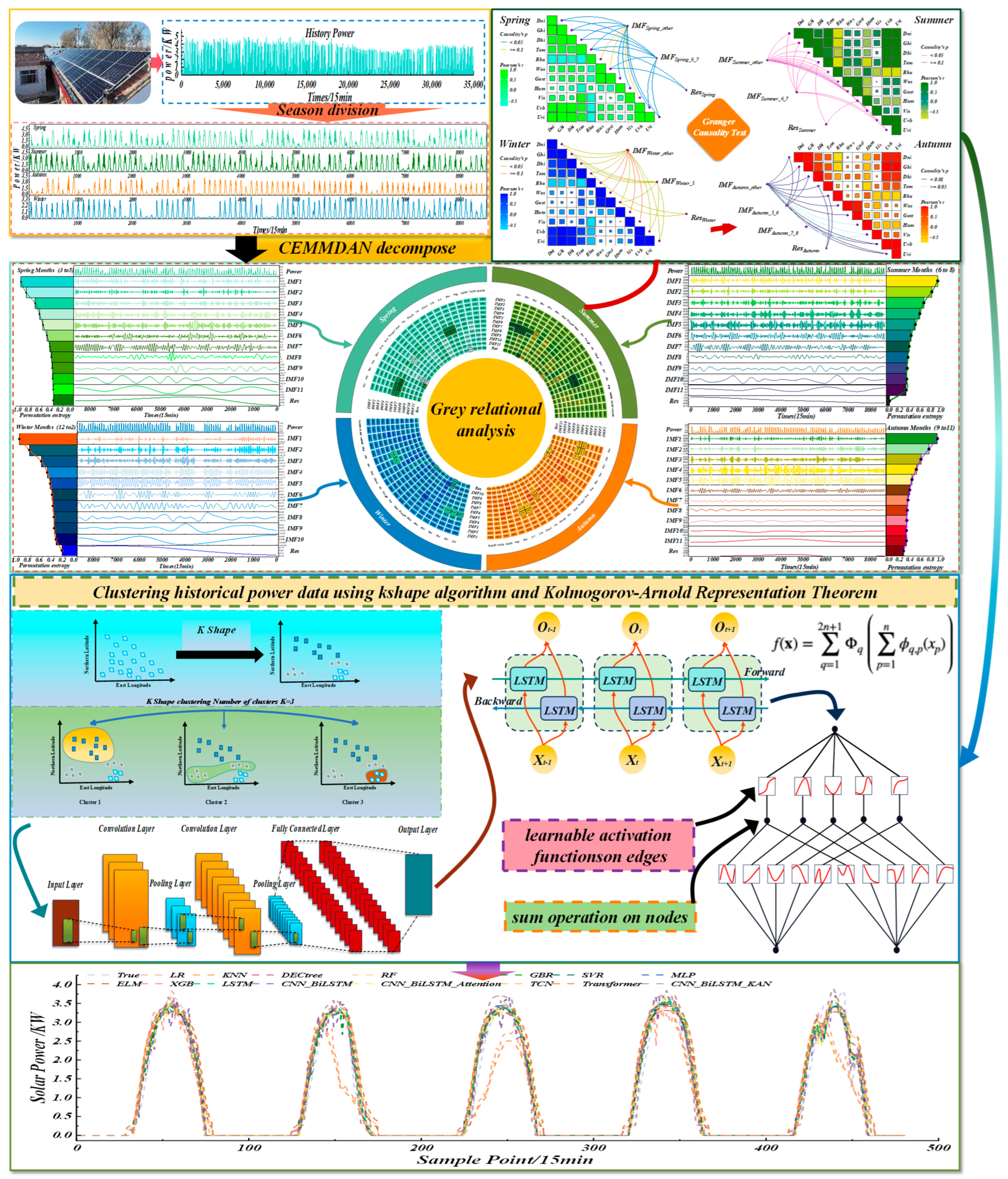
Based on the above method, a photovoltaic power short-term forecasting model is proposed by combining the data preprocessing process with a neural network model. The model is based on weather process matching and CNN_BiLSTM_KAN. The overall structure of the model is shown in Figure 4, The competing models evaluated against the proposed approach are detailed in

Table 1. Comparison of representative PV-forecasting methods.

Ref.	Core Techniques	Key Strengths	Main Limitations	Typical Application Scenarios
LR [31]	Linear regression + NWP	Ultra-fast; interpretable coefficients	Misses nonlinearity & ramps	Day-ahead coarse scheduling
KNN [32]	Euclidean nearest-day search	Zero training; easy to deploy	Storage grows with data; metric sensitive	Small residential PV
DECtree [33]	Single CART on raw features	Human-readable rules	High variance; over-fits noise	Exploratory analysis
RF [34]	Bagging CART ensemble	Robust to outliers; handles interaction	Biased toward majority weather class	Regional fleet forecasting
GBR [35]	Gradient-boosting trees	Captures complex nonlinearity	Slow; hyper-parameters sensitive	Utility short-term markets
SVR [36]	RBF-kernel SV regression	Convex optimum; global solution	Quadratic memory; kernel choice critical	Limited-data sites
MLP [37]	2-layer feed-forward	Simple deep baseline	Vanishing gradients; needs tuning	Research baseline
ELM [38]	Random hidden neurons	Extreme training speed	Random weights → unstable	Ultra-fast prototype
XGB [39]	Boosted trees with regularization	state-of-the-art tabular accuracy	Requires careful early-stopping	Commercial forecasting
LSTM [40]	Vanilla LSTM	Long-term temporal memory	No exogenous causality; over-fits ramps	Single-site hourly
CNN_ BiLstm [41]	1-D CNN + BiLSTM	Local + global spatio-temporal	Fixed topology; no weather-type filter	Day-ahead bidding
CNN_BiLstm_Attention [42]	+ Self-attention	Focus on key time-steps	Attention noise; extra parameters	Research benchmark
TCN [43]	Dilated causal CNN	Long receptive field; parallel training	Struggles with seasonal drift	Intra-day trading
Transformer [44]	Encoder–decoder self-attention	Captures global dependencies	Data-hungry; quadratic complexity	Large-scale farms
The proposed methodology	CEEMDAN-GRA-NGC + K-shape + CNN-BiLSTM-KAN	Season-weather matched; causal feature pruning; interpretable KAN	Higher pre-training time	Distributed rooftops with scarce data and fast ramps

. And the specific steps are as follows:

Step 1: Seasonal split

Divide the PV-power dataset by season. For each season, apply CEEMDAN to decompose the historical power series into IMFs, compute the gray relational grade between every IMF and the meteorological variables, and merge IMFs with highly similar driving features to obtain a compact set of reconstructed components.

Step 2: Two-stage feature selection

(1)

Gray-relational filtering: for each IMF, retain the weather variables whose correlation exceeds a season-specific threshold; the intersection of these per-IMF sets yields the first-stage candidate pool.

(2)

Nonlinear causality test: run a convergent-cross-map test between every reconstructed components and the first-stage candidates, keeping only variables with statistically significant causal influence to form the final input set.

Step 3: K-shape weather clustering and hybrid forecasting

Cluster the samples into weather regimes (sunny, cloudy, rainy, etc.) with K-shape. For each regime, build a dedicated CNN-BiLSTM that fuses the two-stage-selected features of every reconstructed components; feed the high-dimensional latent representation into a KAN network to generate the reconstructed components-level forecast.

Step 4: Recomposition and evaluation

Linearly sum the reconstructed components forecasts to obtain the final PV-power prediction. Accuracy is quantified with MAPE, RMSE and R² against the measured power, demonstrating the scientific validity of the proposed framework.

Across the reviewed pipeline, most existing approaches treat “season” and “weather process” separately or simply concatenate meteorological features, leading to sub-optimal representation of intra-day ramps and seasonal transition anomalies. The proposed framework explicitly couples seasonal decomposition, causal feature selection and shape-based weather clustering, thereby reducing the common error amplification under fluctuating irradiance regimes.

3. Experiments and Analysis

3.1. Data Description and Preprocessing

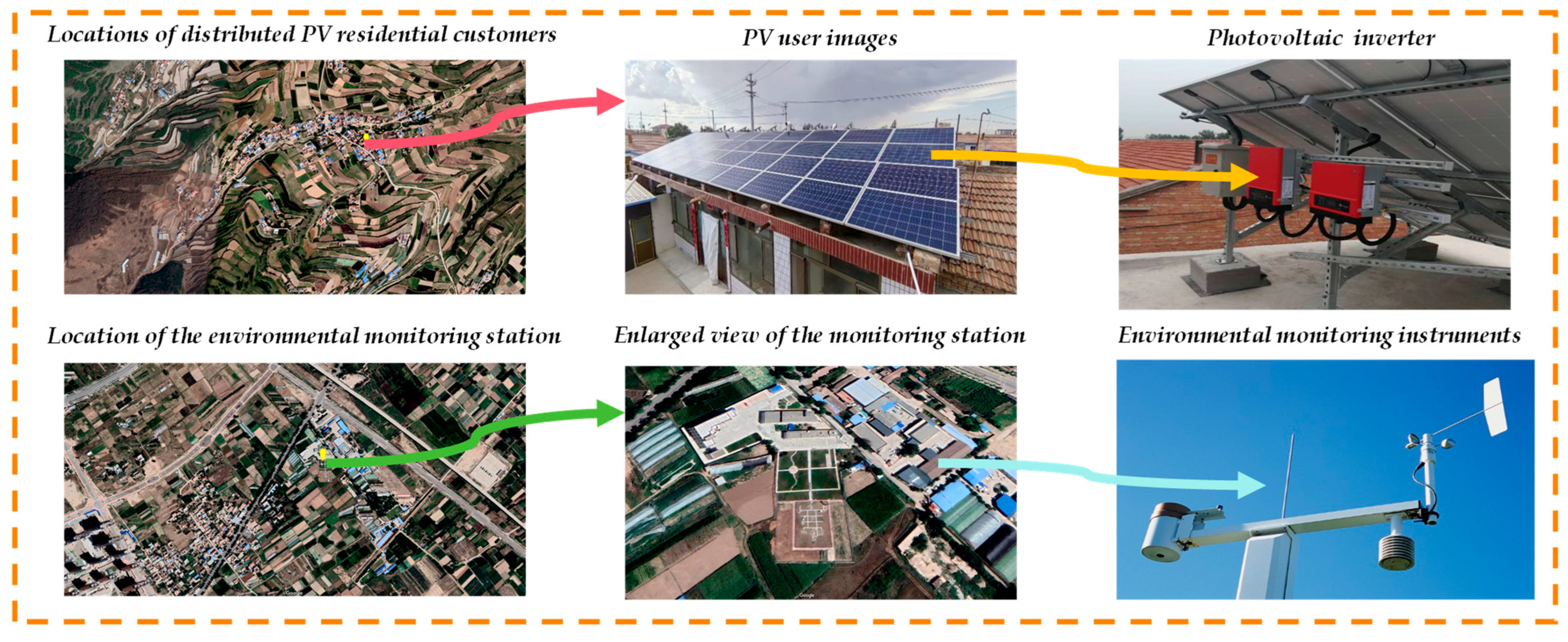
The dataset is derived from the actual generation and operation data of distributed PV users in a certain province. The geographic locations of the distributed PV residential users and the data-acquisition devices are illustrated in Figure 5. The rated installed capacity of the photovoltaic power station is 5 kW. The dataset spans from 00:00 on 1 March 2021, to 23:45 on 1 February 2022. For the purpose of weather classification and power forecasting, the data is divided into four seasonal time periods: spring (March-May), summer (June-August), autumn (September-November), and winter (December, January, and February). All data is selected from daily measurements between 5:00 and 19:00. The resolution of both power data and NWP (Numerical Weather Prediction) meteorological data is 15 min. The NWP data includes 22 features, including irradiance, temperature, and other meteorological variables. Nighttime solar radiation values, which are zero, are removed from the data to ensure synchronization between the NWP and power data. In addition, missing values in the dataset are filled using the mean imputation method. Each seasonal dataset is divided into a training set and a test set, with the training set and test set accounting for 80% and 20% of the data, respectively, for each season.

As shown in Figure 5. The photovoltaic inverter output-power data were recorded, while an environmental monitoring instruments measured air temperature, humidity, pressure, wind speed, wind direction, tilted global irradiance, horizontal global irradiance, horizontal direct irradiance, horizontal diffuse irradiance, and module back-surface temperature. NWP meteorological data were provided by the numerical weather forecast service purchased by the project owner.

3.2. Data Decomposition and Feature Mining

3.2.1. Data Decomposition and Permutation Entropy Fusion

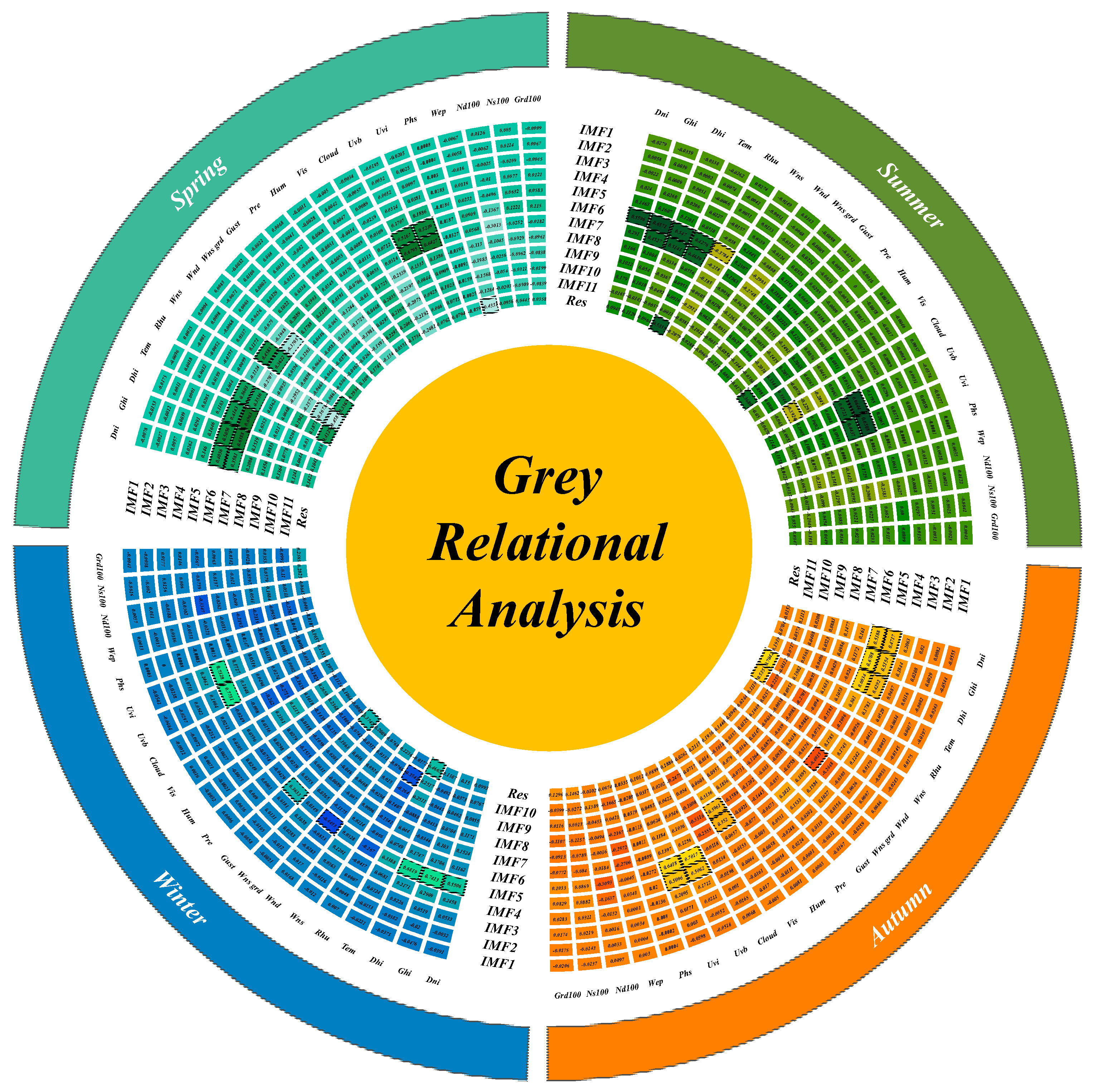
Due to seasonal differences, in spring and autumn, when precipitation events are less frequent and weather systems are relatively stable, the modal curves often exhibit smooth, monotonically decreasing trends. In contrast, in summer and winter, when rain and snow events are frequent and weather processes are complex and variable, the modal curves show significant volatility and nonlinear changes. Traditional correlation methods overlook seasonal factors and fail to consider the correlation between the local changes in nonlinear features and modes across different seasons. To address this issue, this study uses gray relational analysis to evaluate the significance of meteorological features and IMF components for each season, and calculates the correlation between the IMF and weather features based on the decomposition. As shown in Figure 6, the degree of correlation between each modal component and each meteorological element is not consistent. Positive values indicate a positive correlation, meaning the IMF component increases as the associated weather factor value increases. Negative values indicate a negative correlation, meaning the IMF component decreases as the associated weather factor value increases. Therefore, this study focuses only on positively correlated features, selecting weather features with a correlation degree greater than 0.35 and their corresponding modal components as the research objects.

In spring, with the rise in temperature and the extension of daylight hours, strong seasonal gusts are also present. The modal components IMF6 and IMF7 are highly correlated not only with Dni, Ghi, Dhi, Tem, Ubv, and Uvi, but also with wind speed feature Wns. In contrast, the residual component Res is strongly correlated only with Tem and Wns. In summer, high temperatures are often accompanied by thunderstorms, and there is a strong correlation between Dni, Ghi, Dhi, Tem, Ubv, Uvi, and IMF6 and IMF7. The Res component shows a high correlation with Tem and Hum, but a weak correlation with wind speed. In autumn, rainfall decreases, cloudy weather is less frequent, and there is a large temperature difference. Tem, Wns, and Hum exhibit weak correlations or no correlation with IMF5 and IMF6, while Vis shows a strong correlation with IMF7 and IMF8. The Res component for this season is highly correlated with Tem and Rhu. In winter, snowfall causes a drop in temperature, and snow cover on the PV panels reduces their efficiency. IMF5 is highly correlated with Dni, Ghi, Dhi, Gust, Ubv, and Uvi, while showing a weak correlation with Tem. The modal component most highly correlated with Tem and Gust is Res. These results indicate that the modal components, which show high correlations with multiple weather elements, better reflect the frequency and fluctuation characteristics of weather changes during the seasonal transition, while the Res component mainly represents the overall trend of meteorological factors evolving with the seasons. Overall, in all seasons, the correlation between IMF components and Dni, Ghi, Dhi, Ubv, and Uvi is significantly stronger than with other non-negative correlation features. The modal components related to meteorological features with a correlation of less than 0.35 show less apparent variation patterns.

To reduce the computational load during the grouping modeling process and decrease the input data dimensions, the modal components with high correlation (r > 0.35) for the same features in each season are reorganized. Modal components with low correlation (0 < r < 0.35) are integrated into a new modal. As shown in Figure 7, in spring, IMF6 and IMF7 are integrated into IMF_{Spring_6_7}, while Res remains unchanged, and the remaining components are integrated into IMF_{Spring_other}. In summer, the components are integrated into IMF_{Summer_6_7}, IMF_{Summer_other}, and Res_Summer. In autumn, they are integrated into IMF_{Autumn_5_6}, IMF_{Autumn_7_8}, IMF_{Autumn_other}, and Res_Autumn. In winter, the components are integrated into IMF_{Winter_5}, IMF_{Winter_other}, and Res_Winter.

3.2.2. Feature Analysis Based on Causal Association

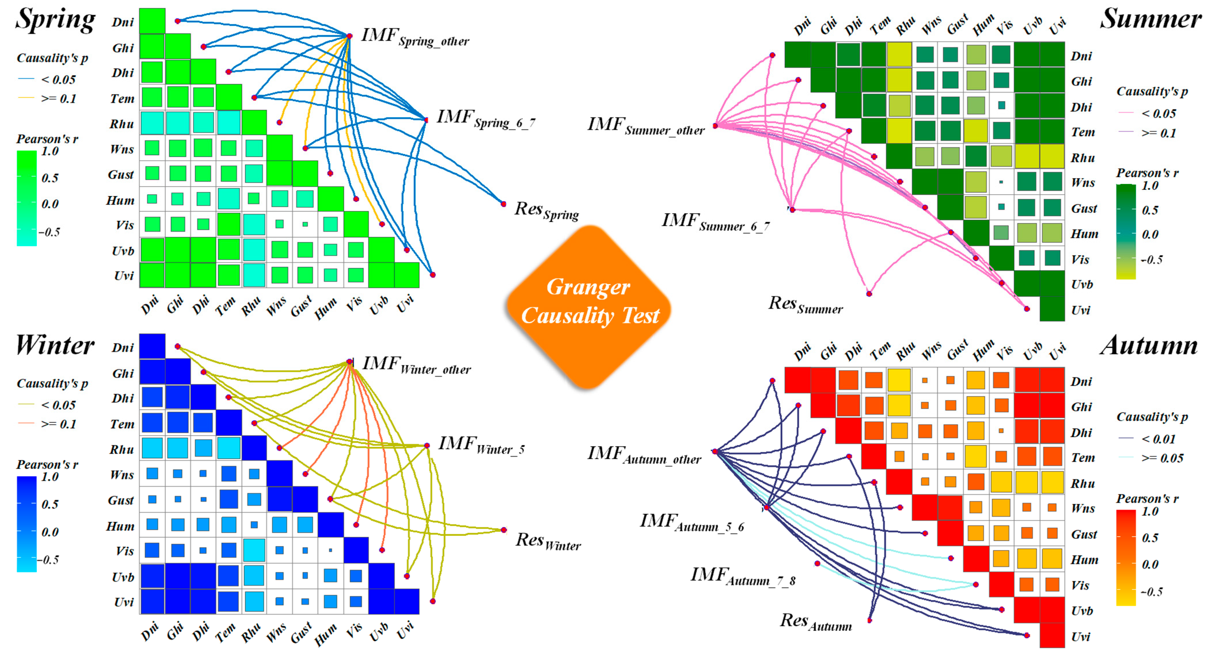
As shown in the causal heatmap in Figure 8, the seasonal heatmap matrices are calculated based on the correlation coefficients between features highly associated with the IMF components. The different colored curves in the figure represent the significance levels of the associated features to the reconstructed components, indicating whether there is a Granger causal relationship between the feature and the reconstructed component. From the causal curves for each season, it can be observed that among the 11 highly associated features, six indicators: Dni, Ghi, Dhi, Tem, Ubv, and Uvi are significantly associated with all four seasons, as shown in

Table 2. Nonlinear Granger causality test results.

Feature (p-Value)		Dni	Ghi	Dhi	Tem	Rhu	Wns	Gust	Hum	Vis	Uvb	Uvi
Spring	IMFSpring_other	0.0061	0.0013	0.0004	0.0207	0.1831	0.5066	0.0883	0.1025	0.5940	0.0038	0.0072
	IMFSpring_6_7	0.0035	0.0077	0.0081	0.0372	/	0.0274	/	/	/	0.0004	0.0094
	RESSpring	/	/	/	0.0289	/	0.0017	/	/	/	/	/
Summer	IMFSummer_other	0.0008	0.0068	0.0089	0.0345	0.1269	0.0316	0.0688	0.0318	0.8473	0.0020	0.0047
	IMFSummer_6_7	0.0056	0.0046	0.0021	0.0071	/	/	/	/	/	0.0053	0.0018
	RESSummer	/	/	/	0.0503	/	/	/	0.0285	/	/	/
Autumn	IMFAutumn_other	0.0035	0.0036	0.0013	0.0656	0.0060	0.1565	0.0113	0.4971	0.7401	0.0088	0.0009
	IMFAutumn_5_6	0.0086	0.0007	0.0035	/	/	/	/	/	/	0.0073	0.0063
	IMFAutumn_7_8	/	/	/	/	/	/	/	/	0.0099	/	/
	RESAutumn	/	/	/	0.0957	0.0040	/	/	/	/	/	/
Winter	IMFWinter_other	0.0019	0.0012	0.0028	0.1045	0.4622	0.9949	0.0019	0.9922	0.9988	0.0006	0.0011
	IMFWinter_5	0.0042	0.0086	0.0081	/	/	/	0.0049	/	/	0.0062	0.0052
	RESWinter	/	/	/	0.0856	/	/	0.0026	/	/	/	/

Note: “/” represents the weather features filtered out in the first stage of the data reconstruction process.

. However, for the other indicators, such as Rhu, Wns, Gust, Hum, and Vis, their significance varies across different seasons. For example, Wns shows significant effects on IMF_{Spring_6_7}, Res_Spring, and IMF_{Summer_other} in spring and summer, while its significance is relatively low for the reconstructed components in autumn and winter. Rhu only has a significant impact on IMF_{Autumn_other} and Res_Autumn in autumn. In winter, Gust shows a significantly higher significance for the reconstructed components during this season. However, the significance of Vis remains weak across all seasons.

Causality tests reveal that the influence of Wns on reconstructed components declines markedly with seasonal shifts; however, this reduction remains negligible in magnitude. In contrast, the statistical significance of Gust exhibits a clear tendency to fluctuate with ambient temperature. Consequently, we apply a second causal-filtering stage to retain only weather drivers that maintain significant Granger causality with each seasonal IMFs, thereby tailoring the feature set to each season-component pair and sharpening forecasting accuracy.

3.3. Weather Type Classification

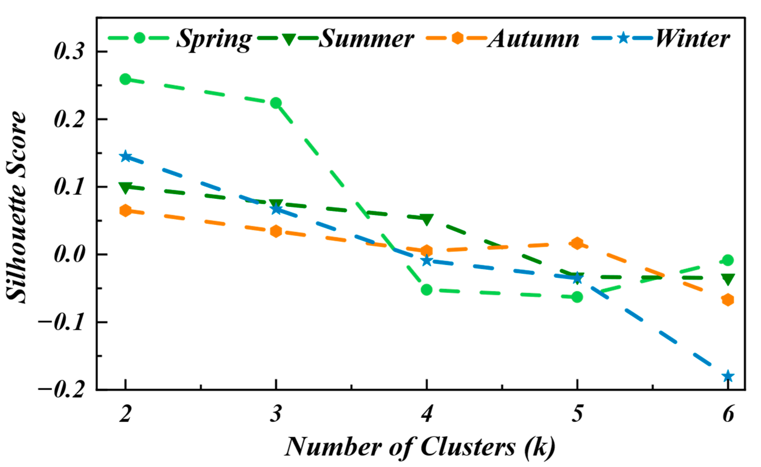
To guarantee that each cluster encapsulates homogeneous weather and power-output behavior, we adopt K-Shape clustering on the pre-processed data. Building on Section 3.2.2, historical PV power series of each season are pooled, while the multi-feature-linked IMFs and the residual Res serve as the clustering input. This procedure exposes latent power-generation regimes and supplies compact, weather-interpreted prototypes for subsequent modeling.

Table 3. The optimal number of clusters for each season.

Season	Spring	Summer	Autumn	Winter
Silhouette Score	0.2238	0.0535	0.0343	0.0670
Number of Cluster	3	4	3	3

shows the optimal number of clusters for each season, determined based on the silhouette coefficient. To determine the optimal number of clusters for each season, we examine the silhouette-coefficient curves shown in Figure 9. In spring the coefficient peaks at k = 3 (0.2238), a value markedly higher than those for the other seasons, indicating that spring weather–power patterns are the most compact; we therefore retain three clusters to balance interpretability and compactness. In contrast, the summer, autumn and winter peaks are only 0.0535, 0.0343 and 0.0670, respectively, all lying in a low-value band that reflects strong weather volatility and large inter-cluster overlap. For these “low-coefficient, high-complexity” cases we adopt a joint “peak + elbow” criterion. Under this rule, the summer curve shows a clearer downward bend at k = 4 than at k = 3, so four clusters are chosen for summer, whereas spring, autumn and winter all exhibit an evident downward elbow at k = 3 with no subsequent abrupt change and are therefore kept at three clusters. This strategy avoids possible over-segmentation that would arise from relying solely on the highest silhouette value and simultaneously ensures sufficient samples within each sub-cluster for the subsequent modeling, thus preserving both physical interpretability and predictive stability. Figure 10 presents the clustering results based on the optimal number of clusters. Taking summer as an example, the K-Shape algorithm visually divides the power principal component sequences into four clusters based on the shape of the curves. Significant differences exist between the clusters: Cluster 1 has a relatively flat power curve, Cluster 2 exhibits varying power amplitudes due to weather changes, Cluster 3 shows large fluctuations and strong volatility with a generally low amplitude, and Cluster 4’s power curve changes are primarily caused by equipment failures or human factors, rather than meteorological influences. To unify the weather type classification and simplify the modeling process, the curves in Clusters 3 and 4 in summer are defined as the same weather type.

Figure 11a Representative power-output sequences for three categories of fluctuating spring-weather events. (b)–(j) Daily normalized profiles of the nine NWP variables (DNI, GHI, DHI, Tem, Wns, Gust, Hum, Uvb, Uvi) that were identified as highly significant by the causality tests for each event.The trend of power fluctuations is similar to the variations in Dni, Ghi, Dhi, Ubv, and Uvi, while the stable fluctuation trend usually corresponds to clear sky weather. However, significant fluctuations can also occur, which can be used as a standard to measure photovoltaic output levels for different weather processes. However, Tem and Wns more significantly reflect the degree of weather fluctuations. The speed of cloud movement is constrained by changes in wind speed, and large fluctuations in wind speed typically show greater variability within a single day. Small fluctuations exhibit certain variations, but sunny-like weather almost never shows long-term wind speed or temperature fluctuations, maintaining a stable low wind speed throughout the day. Humidity also reflects the level of photovoltaic output fluctuations on that day. Under conditions with higher solar radiation, PV panels generate more efficiently, while Gust shows the opposite trend, with lower values corresponding to higher PV output efficiency.

3.4. Predictive Error Evaluation Metrics

This paper uses three evaluation indicators to evaluate the prediction accuracy, including root mean square error (RMSE), mean absolute error (MAE) and R-square (R²). RMSE and MAE are not affected by the scale of the predicted value. The coefficient of determination R² measures the proportion of the variance of the true value that the predicted value can explain. Generally speaking, models with lower RMSE, MAE and higher R² are considered to have better prediction performance. The calculation formulas are:

$$RMSE=\sqrt{{\displaystyle \frac{1}{n}}{{\displaystyle \sum _{i=1}^n\left(\frac{P_{Mi}-P_{Pi}}{C_i}\right)}}^2}$$

(29)

$$MAE={\displaystyle \frac{1}{n}}{\displaystyle \sum _{i=1}^n\left|P_{Mi}-P_{Pi}\right|}$$

(30)

$$R^2=1-{\displaystyle \frac{{{\displaystyle \sum _{i=1}^n\left(P_{Mi}-P_{Pi}\right)}}^2}{{\displaystyle \sum _{i=1}^n{\left(P_{Mi}-P_{Ni}\right)}^2}}}$$

(31)

where n is the total number of samples, the actual power at time i is expressed as $P_{Pi}$, the predicted power at time i is $P_{Mi}$, the normalized value at time i is $P_{Ni}$, $C_i$ is the power-on capacity at time i.

4. PV Forecasting and Error Analysis

4.1. Comparison Results of Seasonal Models

To verify the rationality, applicability, and effectiveness of the method proposed in this paper, multiple forecasting models were compared. Thirteen commonly used models, including LR, KNN, DECtree, ELM, and others, were selected as comparative algorithms. For a quantitative analysis of forecasting model accuracy, the results for one day from the test dataset were selected for analysis. The test data is categorized into four different seasons, and within each season, the weather is systematically arranged in the order of sunny-like, cloudy, and rainy days.

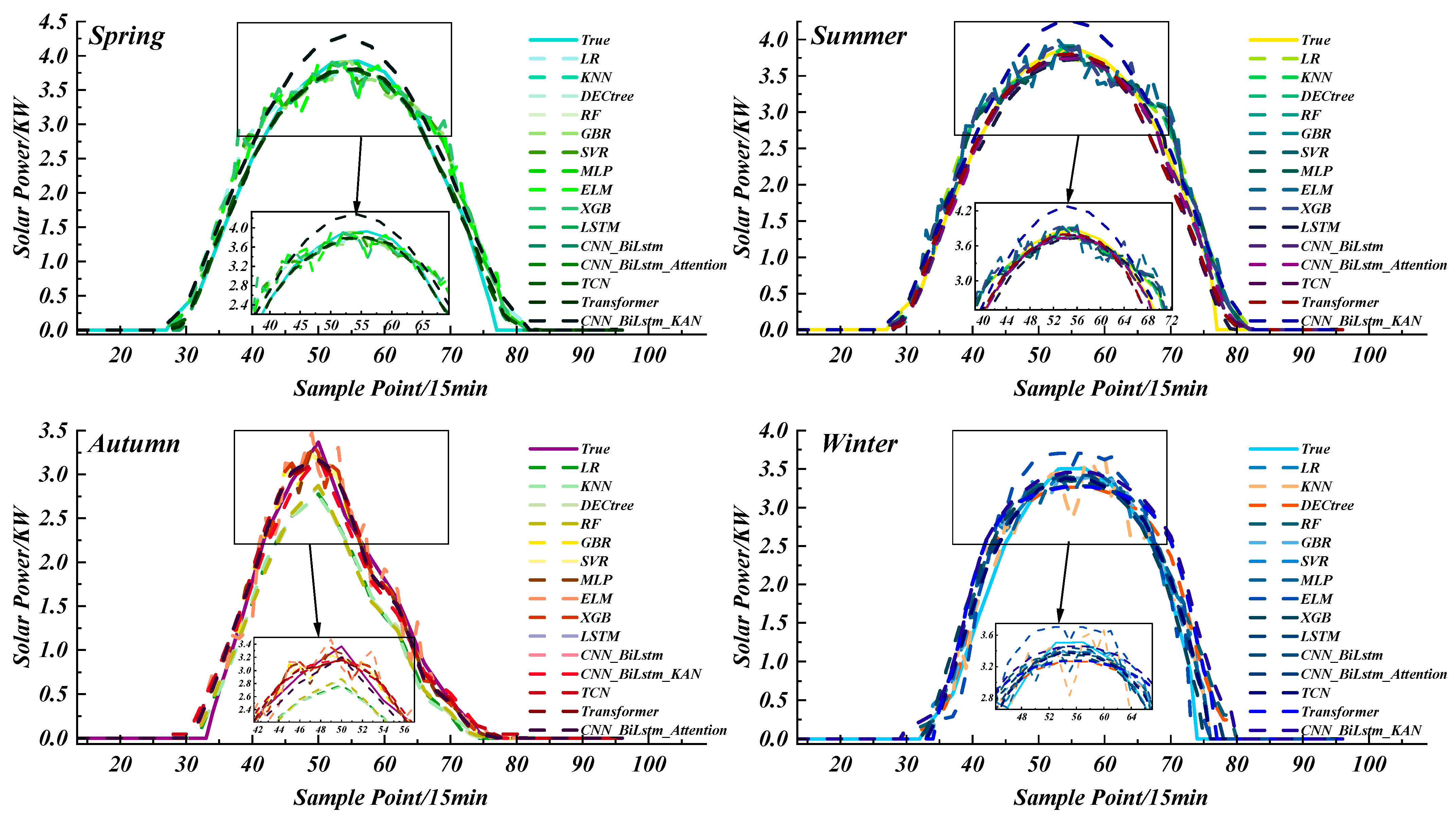
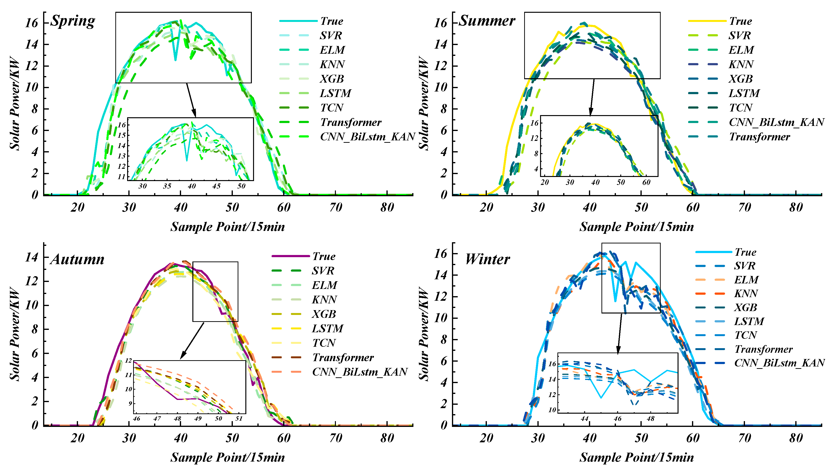
Figure 12 shows the model prediction results for each model in the sunny-like cluster for each season. It can be observed that under clear weather, photovoltaic output curves show relatively small fluctuations and exhibit a stable trend across all seasons. As shown in the error radial plot in

Table 4. Performance Comparison of Different Forecasting Models under Sunny-like Weather.

Model	Index	Spring	Summer	Autumn	Winter	Average
LR	RMSE	17.01%	16.07%	17.31%	18.04%	17.11%
	MAE	12.65%	11.53%	12.61%	11.74%	12.13%
	R2	77.27%	79.28%	78.67%	78.54%	78.44%
KNN	RMSE	14.38%	13.44%	14.69%	14.72%	14.31%
	MAE	13.26%	10.39%	11.55%	10.78%	11.50%
	R2	79.15%	80.58%	79.47%	79.11%	79.58%
DECtree	RMSE	13.78%	15.26%	13.72%	13.95%	14.18%
	MAE	12.39%	11.84%	11.63%	10.63%	11.62%
	R2	80.22%	81.12%	80.77%	80.11%	80.56%
RF	RMSE	14.16%	13.84%	12.62%	13.74%	13.59%
	MAE	12.47%	10.25%	9.12%	10.35%	10.55%
	R2	80.07%	80.67%	81.27%	81.16%	80.79%
GBR	RMSE	15.05%	16.36%	13.45%	14.98%	14.96%
	MAE	11.27%	12.25%	9.49%	12.66%	11.42%
	R2	81.61%	79.94%	80.86%	80.09%	80.63%
SVR	RMSE	13.52%	15.04%	14.84%	12.96%	14.09%
	MAE	11.53%	11.58%	11.47%	10.16%	11.19%
	R2	82.56%	80.27%	81.32%	82.96%	81.78%
MLP	RMSE	13.93%	14.46%	12.89%	11.98%	13.32%
	MAE	11.41%	11.45%	10.71%	9.22%	10.70%
	R2	81.96%	81.61%	82.72%	84.02%	82.58%
ELM	RMSE	15.53%	12.76%	12.08%	10.72%	12.77%
	MAE	12.44%	11.48%	9.54%	8.69%	10.54%
	R2	79.93%	82.27%	84.49%	83.94%	82.66%
XGB	RMSE	12.66%	10.92%	11.45%	11.06%	11.52%
	MAE	10.44%	9.13%	8.55%	10.83%	9.74%
	R2	80.69%	85.22%	83.65%	86.84%	84.10%
LSTM	RMSE	10.76%	9.07%	10.91%	10.61%	10.34%
	MAE	9.42%	7.38%	8.31%	9.56%	8.67%
	R2	82.55%	87.13%	84.95%	86.88%	85.38%
CNN_ BiLstm	RMSE	7.39%	8.81%	9.69%	7.55%	8.36%
	MAE	7.44%	8.88%	6.52%	7.01%	7.46%
	R2	88.55%	89.93%	87.47%	90.54%	89.12%
CNN_BiLstm_Attention	RMSE	6.19%	7.75%	8.98%	5.42%	7.09%
	MAE	6.42%	6.37%	4.59%	5.51%	5.72%
	R2	90.81%	90.17%	88.81%	91.61%	90.35%
TCN	RMSE	5.16%	6.97%	7.16%	5.01%	6.08%
	MAE	5.24%	6.18%	6.37%	4.59%	5.60%
	R2	90.95%	89.83%	90.27%	90.68%	90.43%
Transformer	RMSE	6.83%	5.44%	6.33%	4.58%	5.80%
	MAE	5.33%	5.07%	5.27%	4.81%	5.12%
	R2	91.04%	89.87%	91.54%	89.73%	90.55%
CNN_ BiLstm_KAN	RMSE	4.06%	5.93%	5.88%	3.16%	4.76%
	MAE	5.03%	4.35%	3.62%	4.92%	4.48%
	R2	92.26%	91.42%	91.74%	92.66%	92.02%

, under the sunny-like cluster, the CNN_BiLSTM_KAN combined model has the highest prediction accuracy. By decomposing and clustering the data, selecting reasonable weather features and datasets, the method effectively suppresses overfitting of the prediction results. As shown in Table 4, for the four seasons, the average RMSE is 4.76% and MAE is 2.25%, both lower than the other 14 comparative models. The average R² value is 92.02%, showing better fit than the other 14 models. The CNN_BiLSTM_KAN combined model shows the closest prediction values to the actual values around noon, and the prediction effect of the proposed method is the best in the sunny-like cluster.

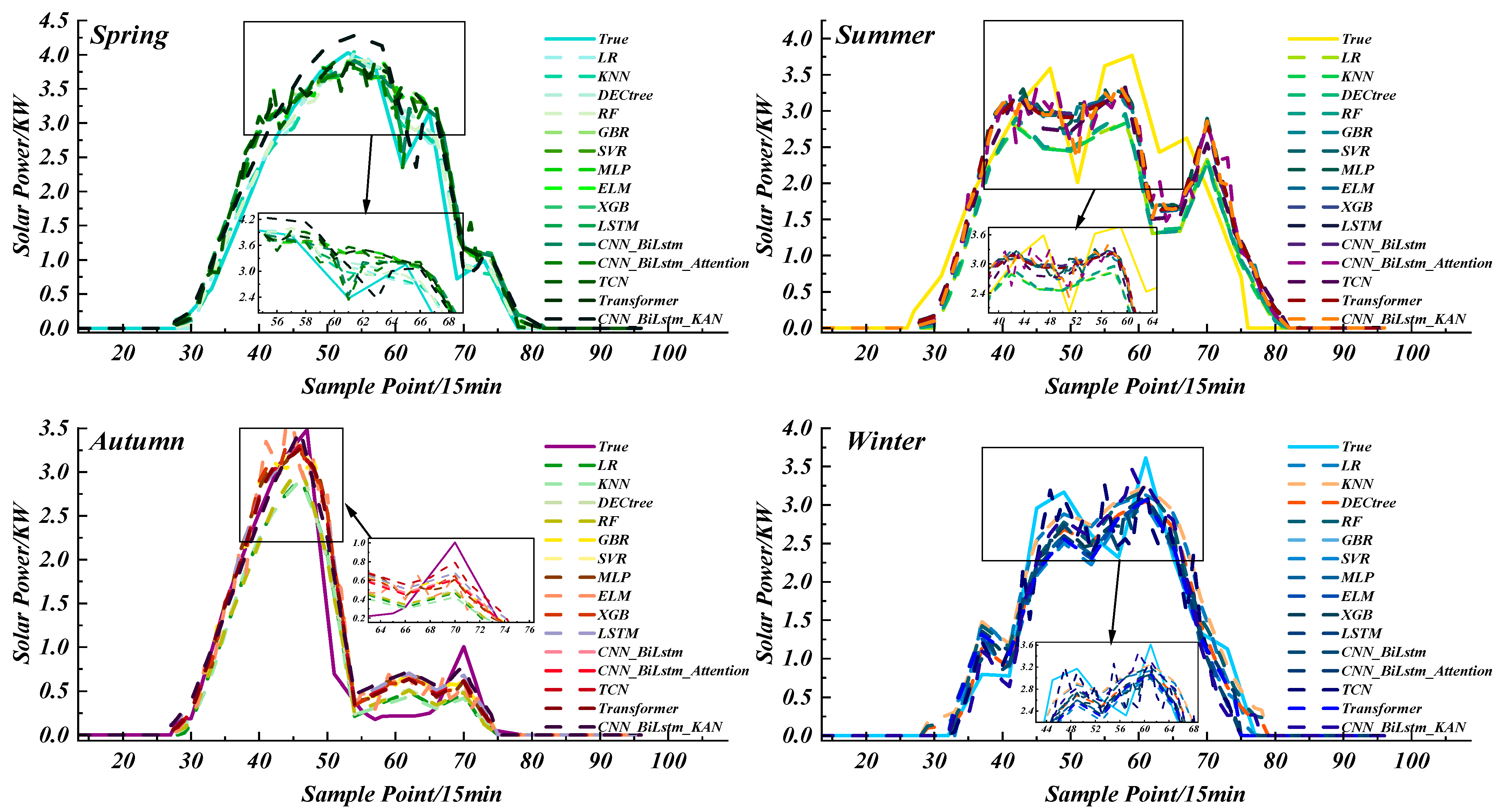
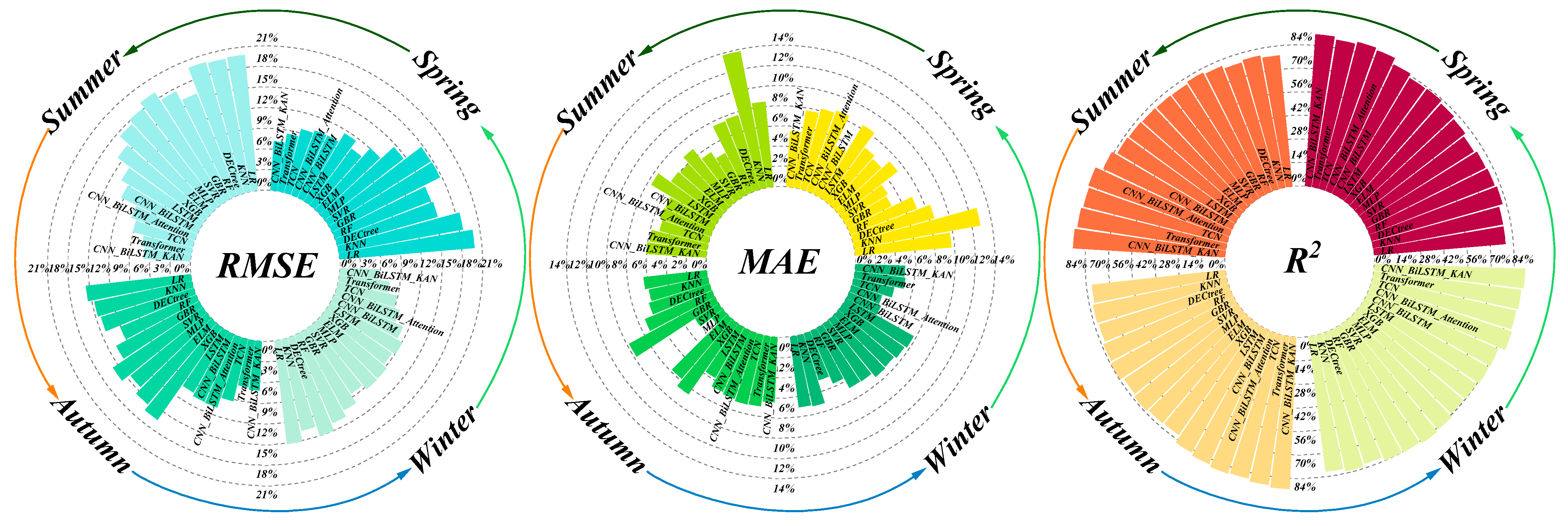
As shown in Figure 13, under the cloudy weather type, the prediction results of the CNN_BiLSTM model closely follow the actual historical data trend, with noticeable small fluctuations. The CNN_BiLSTM_KAN combined model’s prediction curve aligns as closely as possible with the actual data curve, achieving better forecasting results in the presence of many small fluctuations. The error radial plot is shown in Figure 14. In the cloudy weather cluster, the average error metrics for the CNN_BiLSTM_KAN combined model are as follows: RMSE is 6.53%, lower than the other 14 models; MAE is 5.35%, lower than the other 14 models; and R² is 90.51%, higher than the other 14 comparative models. It can be concluded that, in the cloudy weather cluster, the CNN_BiLSTM_KAN combined model has the smallest MAE, the highest accuracy, and the highest coefficient of determination R².

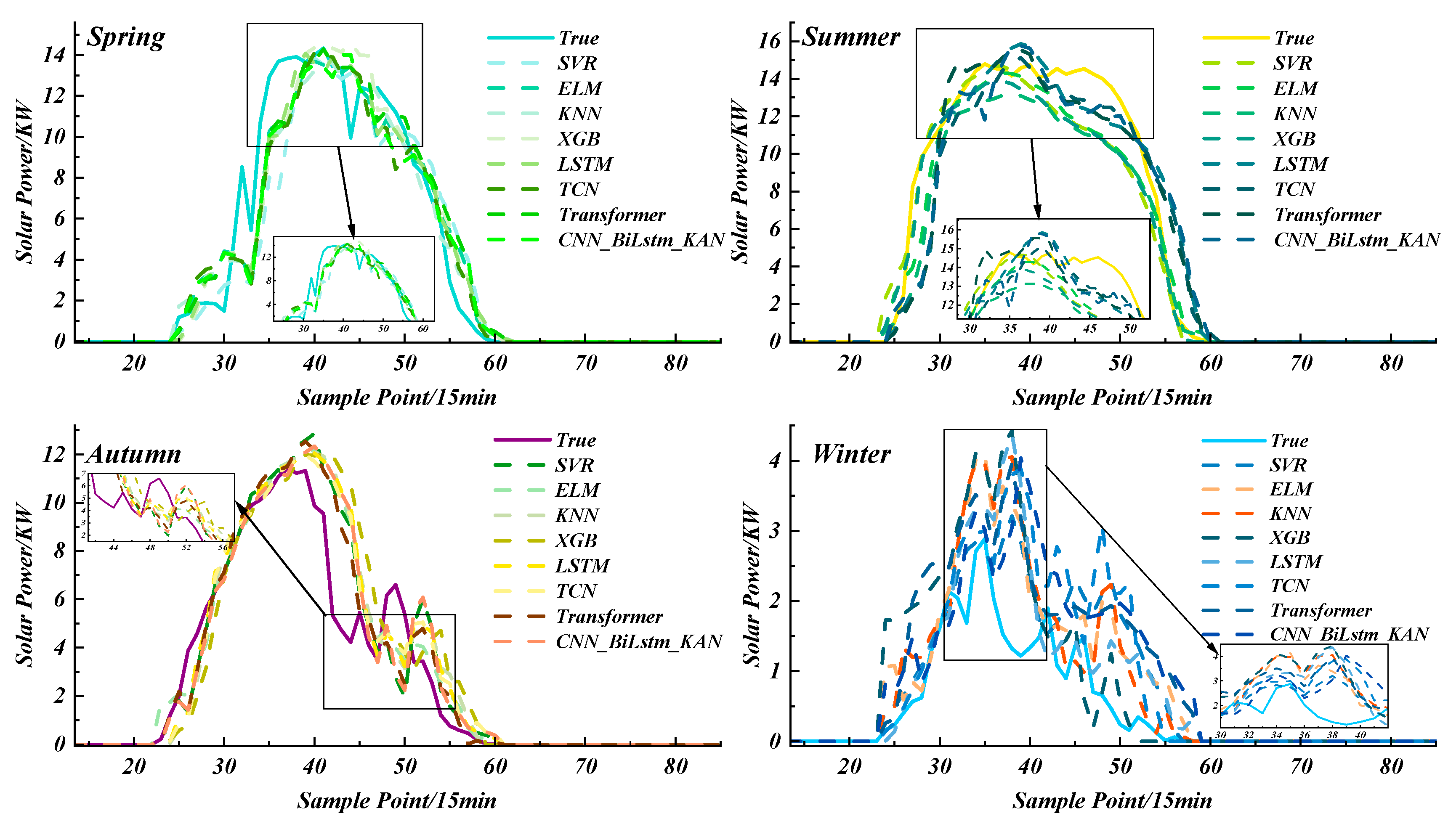
Under the rainy weather type, the output power curve of photovoltaic panels fluctuates irregularly due to sudden changes in irradiance, making power forecasting difficult with traditional machine learning methods. The performance differences between models can be directly attributed to architectural design variations. As shown in the prediction results in Figure 15, The prediction curves of machine learning models are almost linear and do not effectively fit the dynamic trend of actual performance, indicating that they fail to learn the most important features in the data, exhibiting typical overfitting. In contrast, the prediction curves of the CNN_BiLSTM_KAN and CNN_BiLSTM combined models are the closest to the actual values. Both models can follow the changing trend of the actual power curve. When the data fluctuation range is large and the periodic variation in irradiance is not well represented, these models improve the forecasting accuracy, demonstrating the method’s strong generalization capability. Figure 16 compares the error metrics of all models. It can be seen that, under the rainy weather cluster, the CNN_BiLSTM_KAN model’s average error metrics are as follows: RMSE is 6.75%, lower than the other 14 models; MAE is 5.73%, lower than the other 14 models; and R² is 90.74%, higher than the other 14 models. It can be concluded that, under the large fluctuation cluster, the CNN_BiLSTM_KAN combined model has the smallest MAE, the highest accuracy, and the highest coefficient of determination R².

The final output of the model is obtained by stacking the predicted values of the reconstructed sequences. From the above prediction results, it can be seen that under the clear weather cluster, cloudy weather cluster, and rainy weather cluster, the RMSE and MAE of the CNN_BiLSTM_KAN combined model are the smallest, and the coefficient of determination R² is the highest. The proposed model consistently achieves the best results. As shown in

Table 5. Annual average error indicators for various weather types.

Weather Type Label	Sunny-Like			Cloudy Day			Rainy Day
Model	RMSE	MAE	R2	RMSE	MAE	R2	RMSE	MAE	R2
LR	17.11%	12.13%	78.44%	15.94%	7.76%	78.05%	17.58%	7.89%	79.79%
KNN	14.31%	11.50%	79.58%	14.25%	8.61%	78.68%	16.59%	9.95%	80.89%
DECtree	14.18%	11.62%	80.56%	13.91%	7.69%	80.43%	16.11%	6.83%	80.70%
RF	13.59%	10.55%	80.79%	13.52%	7.38%	81.63%	14.27%	6.89%	81.90%
GBR	14.96%	11.42%	80.63%	12.02%	6.28%	81.54%	15.51%	6.51%	82.33%
SVR	14.09%	11.19%	81.78%	12.69%	7.03%	81.89%	15.98%	5.04%	81.45%
MLP	13.32%	10.70%	82.58%	12.23%	6.60%	82.39%	14.85%	5.67%	82.18%
ELM	12.77%	10.54%	82.66%	11.17%	7.13%	83.61%	14.30%	6.79%	81.87%
XGB	11.52%	9.74%	84.10%	11.97%	8.87%	85.12%	13.48%	7.19%	82.34%
LSTM	10.34%	8.67%	85.38%	11.69%	6.92%	84.93%	11.82%	7.35%	83.88%
CNN_BiLstm	8.36%	7.46%	89.12%	9.96%	5.80%	88.61%	11.03%	5.15%	85.72%
CNN_BiLstm_Attention	7.09%	5.72%	90.35%	8.91%	6.22%	88.80%	10.10%	5.97%	89.02%
TCN	8.11%	5.11%	91.13%	8.01%	5.98%	89.23%	9.24%	5.15%	90.18%
Transformer	6.37%	5.02%	90.77%	7.65%	5.42%	90.20%	7.78%	5.98%	91.22%
CNN_BiLstm_KAN	4.76%	4.48%	92.02%	6.53%	5.35%	90.51%	6.75%	5.73%	90.74%

, the average error metrics for each weather type over the entire year indicate that the proposed method demonstrates excellent generalization ability and low prediction error when processing the data. The performance advantage of the CNN_BiLSTM_KAN model can be attributed to its unique architecture. The convolutional layer effectively captures local features, the BiLSTM component models bidirectional time dependencies, and the KAN attention mechanism dynamically highlights important time steps and features. As shown in

Table 6. Operating parameters and runtime data for each model.

Model	Key Parameter(s)	Value	Train Samples (Days)	Time(s)
LR	fit_intercept	True	288	0.002
KNN	n_neighbors, weights	10, distance	288	0.006
DECtree	max_depth, min_samples_split	None, 10	288	0.185
RF	n_estimators, max_depth, min_samples_split	500, 30, 5	288	0.093
GBR	n_estimators, learning_rate, max_depth	400, 0.05, 5	288	9.5171
SVR	Kernel, C, ε	RBF, 100, 0.01	288	12.1877
MLP	hidden_layer_sizes, activation, solver, learning_rate_init	(128, 64), ReLU, Adam, 1 × 10−3	288	7.1446
ELM	n_hidden, activation_func	500, sigmoid	288	1.4033
XGB	n_estimators, max_depth, learning_rate, subsample	500, 6, 0.05, 0.8	288	0.055
LSTM	hidden_units, layers, dropout, optimizer, learning_rate, epochs	128, 2, 0.2, Adam, 1 × 10−3, 30	288	133.0592
CNN_ BiLstm	CNN filters, kernel_size, BiLSTM units, layers, dropout, epochs	64, 3, 128, 2, 0.2, 30	288	183.4738
CNN_BiLstm_Attention	Same as CNN_BiLstm, attention heads, epochs	-, 8, 30	288	80.389
TCN	dilated causal filters, kernel size, dilation rates, dropout, optimizer, learning_rate, epochs	64, 3, [1,2,4,8], 0.2, Adam, 1 × 10−3, 30	288	758.939
Transformer	d_model, n_heads, e_layers, d_layers, d_ff, dropout, positional encoding, optimizer, earning_rate, epochs	128, 8, 2, 1, 256, 0.1, sine, Adam, 1 × 10−4, 30	288	483.192
CNN_ BiLstm_KAN	Same as CNN_BiLstm, KAN basis functions, polynomial order, λ_reg, epochs	-, 16, 3, 1 × 10−4, 30	288	436.6235

, although the proposed approach requires slightly more offline-training time, once training is complete its inference phase is markedly faster and achieves the lowest RMSE and MAE on every seasonal-weather subset. This demonstrates not only computational efficiency but also multi-scale robustness under diverse climatic conditions, highlighting its stability when handling data across different scales. The R² value further confirms the model’s high fit with the data, indicating that it can more effectively explain the changes in power trends compared to other competing models. This integrated approach enables the model to effectively learn and represent complex time patterns, thereby improving the accuracy and stability of predictions. This demonstrates that the short-term power forecasting method for distributed photovoltaics based on the proposed approach is universal, whether in clear skies with small power fluctuations or in extreme weather conditions with large power fluctuations.

All models are implemented in Python 3.9 (scikit-learn 1.3, TensorFlow 2.11) and trained on identical hardware (Intel i7-12700K, 32 GB RAM, RTX-3080 10 GB, Intel, Santa Clara, CA, USA).

4.2. Ablation Study

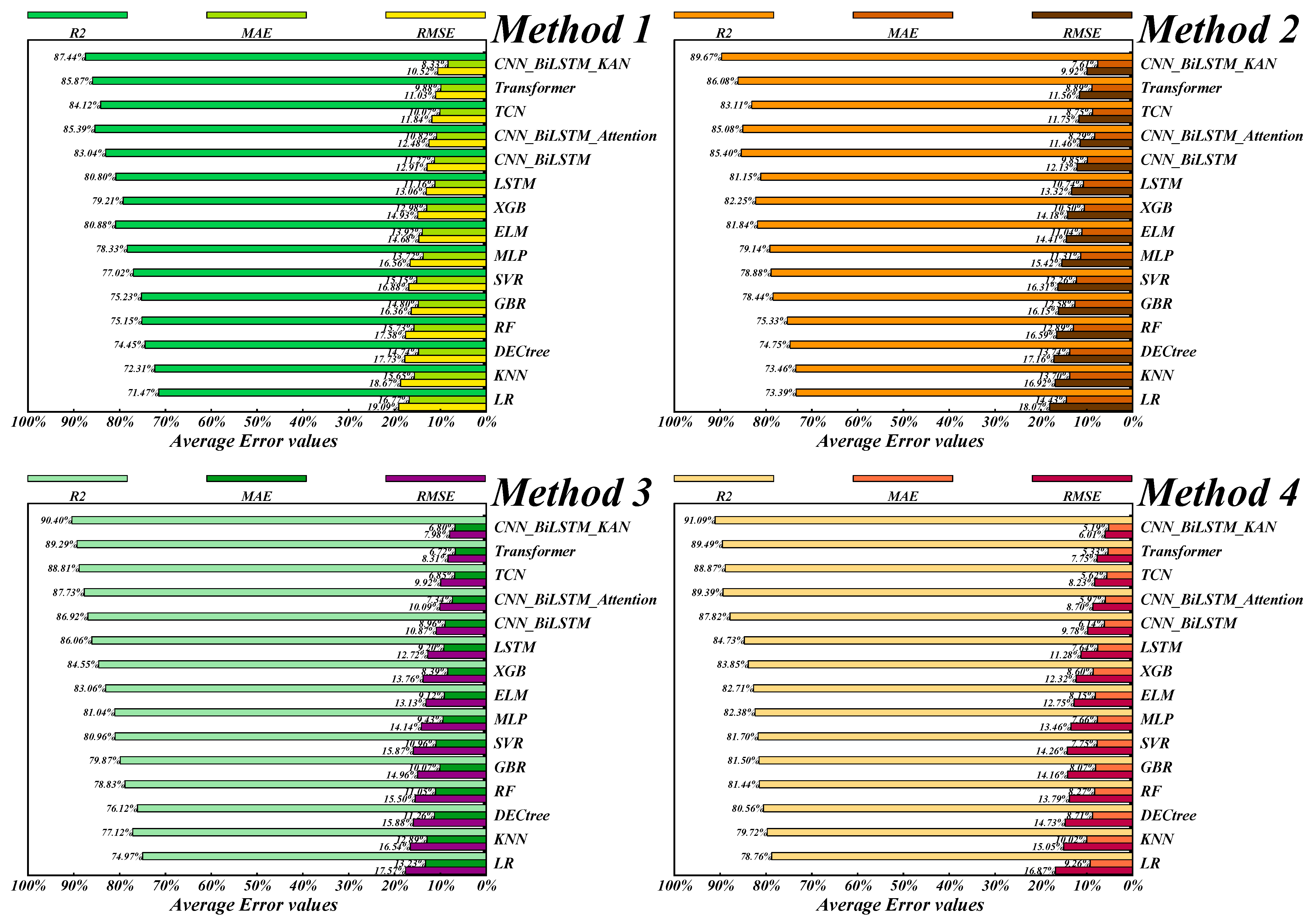
In order to prove the superiority of the method proposed in this paper, several other methods were configured as benchmarks for comparison during the experiment, and the average error indicators of each model throughout the year were compared and analyzed. In the first method, the data for the whole year is not divided into seasons, and the historical power is combined with all NWP characteristics of the traditional time series prediction method; in the second method, the traditional time series direct prediction method divided by season is used; the third method only focuses on the problem of weather feature matching, does not divide the weather type, and only combines the prediction method of data decomposition and feature mining on the basis of the second method; the fourth method is the method of this paper.

In this study, the model predicts using the methods described above. The training set includes samples of three types of fluctuation processes, and five days are selected as the test set. Figure 17 shows the power prediction results for the three fluctuating weather processes. Compared with the other three methods, the proposed method consistently demonstrates higher accuracy in various prediction tasks, with significant improvements in average error metrics. Among the first three methods, the prediction errors for any weather process are relatively larger compared to Method 4. Method 2’s prediction RMSE is 0.6% lower on average than Method 1, which predicts without season division, MAE is 0.72% lower on average, and R² is 2.23% higher on average. This proves that seasonal modeling and data decomposition methods can effectively reduce the noise interference in the prediction model, providing more robust and reliable results. Method 3’s prediction RMSE is 1.94% lower on average than Method 2, MAE is 0.81% lower on average, and R² is 0.73% higher on average, which shows that effective weather features help the model better adapt to varying conditions, enhancing its adaptability and accuracy. In Method 4, the proposed method’s prediction RMSE is 1.97% lower on average than Method 3, which does not use weather type division, MAE is 1.61% lower on average, and R² is 0.69% higher on average. This proves that the modeling approach of dividing weather types and matching weather features using CNN_BiLSTM_KAN can significantly improve short-term photovoltaic power forecasting accuracy under fluctuating weather events, demonstrating the effectiveness of the proposed method.

4.3. Influence of the Gray Relational Threshold

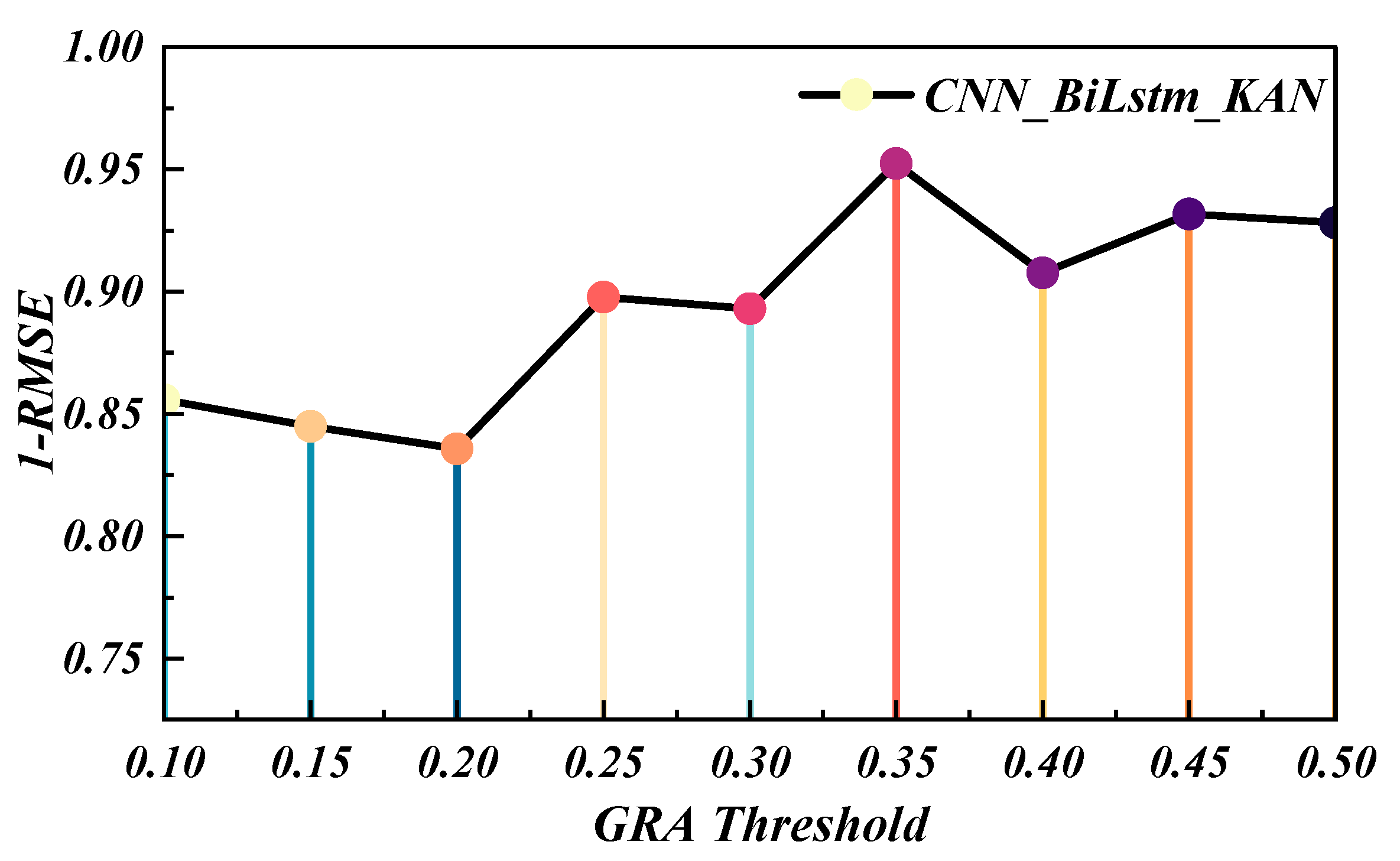
The level of gray correlation directly determines which features are retained during modal reconstruction and the second-stage screening, while the choice of threshold strongly affects training performance. Therefore, we run the model under a series of thresholds, compute the corresponding forecasts, and plot the RMSE-versus-threshold curve; the minimum RMSE identifies the optimal gray-relation threshold for our scenario. This curve is shown in Figure 18.

As shown in Figure 18, the prediction error exhibits a trend of first increasing and then decreasing as the gray correlation threshold grows. When the threshold is below 0.35, although there are many optional features, their correlation is low, making it difficult for the model to capture effective information, thus resulting in high error. After exceeding 0.35, the error continues to decrease with the threshold. Although the number of candidate features reduces, the retained variables tend to be consistent and information-concentrated, enabling the model to efficiently extract key features. However, when the threshold is further increased, the number of selectable features drops sharply, insufficient to support adequate training and leading to an increase in error.

4.4. Other-Region Experiments for Distributed-PV User

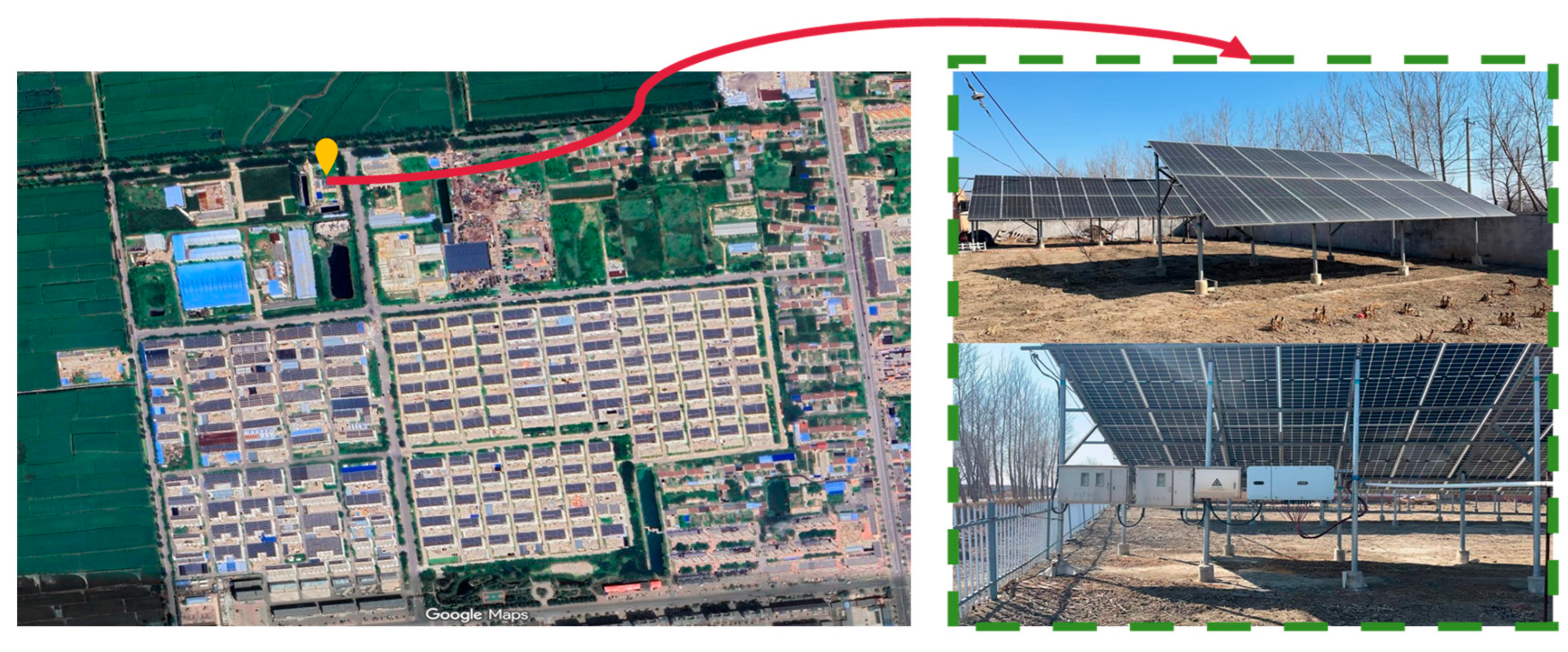
To demonstrate the generality of the proposed method, this study utilizes one-year (3 February 2023 to 4 February 2024.) of photovoltaic (PV) data from a residential distributed-PV user in a city of Liaoning Province. The dataset comprises 15 min PV-power records and corresponding Numerical Weather Prediction (NWP) meteorological variables. The installation has a rated capacity of 16 kW; its geographic location and the power-generation equipment are depicted in Figure 19.

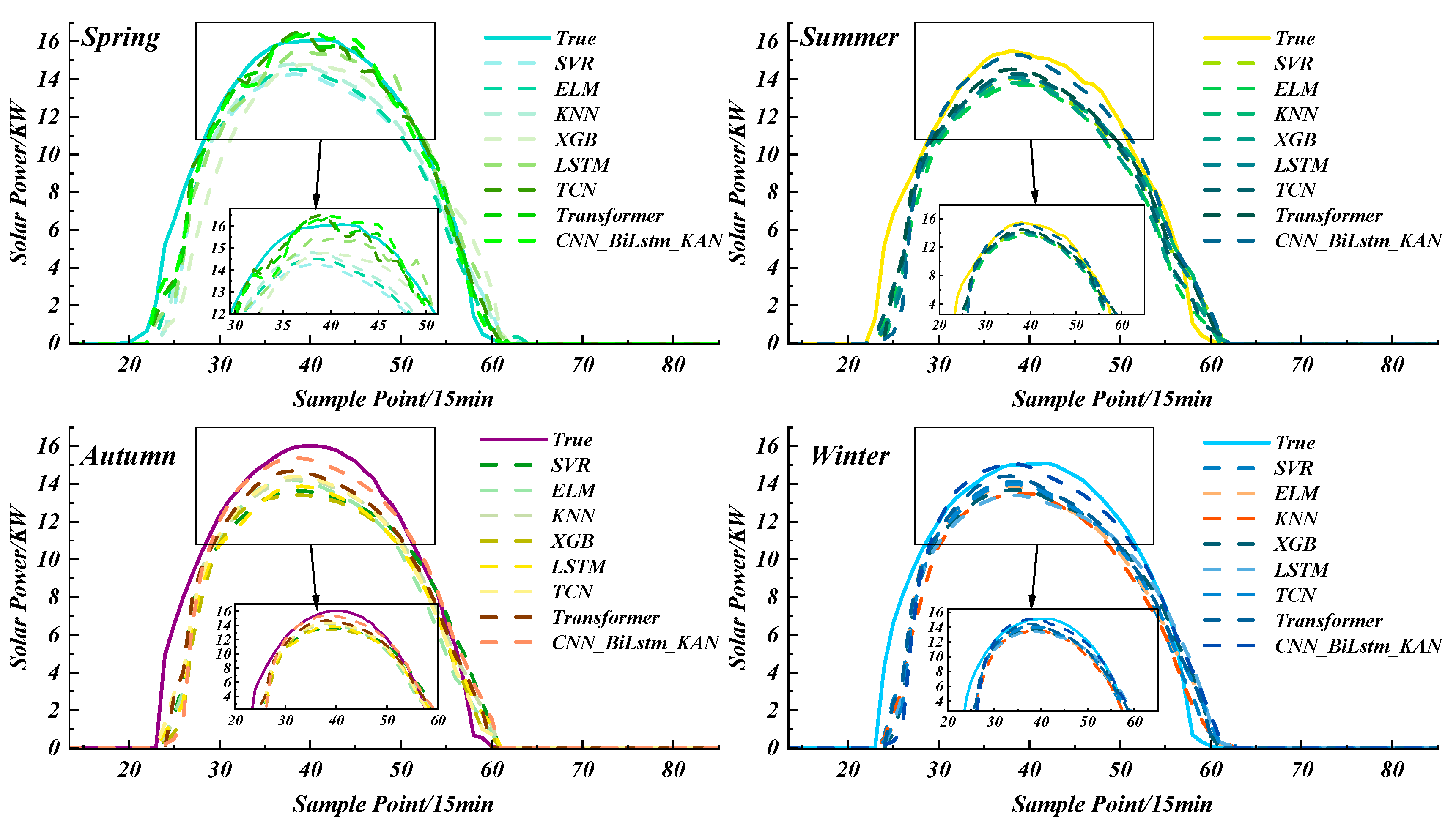
To reduce computational time, this paper selects seven classical machine-learning and deep-learning models as baselines, with all parameters set exactly as listed in Table 6. Figure 20, Figure 21 and Figure 22 compare the seasonal and weather-type curves; it is evident that the proposed forecast curve stays closest to the measured values and accurately tracks PV fluctuations even on cloudy and rainy days, demonstrating a clear advantage. This superiority is further quantified in

Table 7. Annual average error indicators for various weather types in other regions.

Weather Type Label	Sunny-Like			Cloudy Day			Rainy Day
Model	RMSE	MAE	R2	RMSE	MAE	R2	RMSE	MAE	R2
SVR	10.72%	4.86%	84.97%	11.23%	7.99%	75.73%	13.92%	6.25%	84.46%
ELM	10.67%	9.41%	86.93%	11.61%	7.85%	79.13%	12.08%	8.77%	85.47%
KNN	11.85%	8.15%	84.46%	13.12%	8.44%	80.79%	11.45%	9.65%	86.27%
XGB	9.87%	4.17%	89.41%	12.16%	8.73%	82.37%	10.91%	4.74%	86.45%
LSTM	9.99%	7.59%	89.03%	9.59%	7.17%	88.55%	9.69%	5.73%	89.15%
TCN	7.32%	6.68%	88.91%	8.15%	6.92%	88.43%	8.98%	4.82%	89.23%
Transformer	6.17%	5.73%	90.37%	7.98%	6.76%	90.93%	9.02%	5.59%	87.71%
CNN_BiLstm_KAN	6.03%	5.13%	91.12%	7.74%	6.64%	91.42%	8.64%	5.46%	89.32%

, in the three metrics, the proposed method achieves the lowest RMSE and MAE and the highest R², comprehensively confirming its dominance.

5. Conclusions

This paper constructs a short-term forecasting model for distributed PV power and conducts simulation experiments based on actual data from distributed PV users in different provinces, validating the effectiveness of the proposed model. The main conclusions are as follows:

(1)

The CEEMDAN method is used to decompose and reconstruct power data divided by season, revealing seasonal fluctuations within the series. Compared to the data reconstruction method, the prediction model’s RMSE improved by an average of 4.51%, MAE decreased by 3.14%, and R² increased by 3.65%.

(2)

The GRA and NGC methods are used to correlate the time series with weather features for each season, uncovering difficult-to-identify nonlinear relationships between the time series and weather features. Compared to the method without weather type division, the average RMSE for sunny-like, cloudy, and rainy weather environments decreased by 4.69%, 1.93%, and 2.61%, respectively, and the average MAE decreased by 3.77%, 3.15%, and 3.24%. Meanwhile, the average R² increased by 3% to 9%.

(3)

The K-Shape algorithm is used to classify power sequences into weather types, obtaining representative weather event meteorological features and high-precision similar-day datasets. This allows for short-term forecasting of distributed PV power under different weather scenarios, reducing the impact of PV output uncertainty, lowering the data computation load, and improving operational efficiency.

(4)

Compared to traditional machine learning models, the proposed method based on CNN_BiLSTM_KAN demonstrates better prediction performance. CNN_BiLSTM_KAN reduces RMSE by 7.09%, MAE by an average of 2.83%, and increases R² by an average of 8.21% across all seasons and weather types, showing a clear forecasting advantage over traditional models.

These results demonstrate that the method proposed in this paper effectively captures local features and global dependencies in time series data by combining CNN_BiLSTM and KAN networks, reflecting the generality and accuracy of the proposed approach.

6. Future Work

Although the method proposed in this paper significantly improves the power prediction accuracy of distributed photovoltaic stations, this paper does not distinguish between fluctuating weather events in a refined manner. To further improve the power prediction accuracy, a more detailed weather process division is needed. At the same time, the weather process-based division method in this paper is completely dependent on NWP. The NWP forecast accuracy will significantly affect the accuracy of weather event division. Therefore, in the future, we will further consider more detailed weather process analysis and division methods while reducing the dependence of weather process division on NWP so as to improve the overall accuracy of weather process division and power prediction accuracy.

References

1. Yang, M.; Jiang, Y.; Xu, C.; Wang, B.; Wang, Z.; Su, X. Day-ahead wind farm cluster power prediction based on trend categorization and spatial information integration model. Appl. Energy 2025, 388, 125580. [Google Scholar] [CrossRef]
2. Kang, K.; Jia, H.; Hui, H.; Liu, D. Two-stage optimization configuration of shared energy storage for multi-distributed photovoltaic clusters in rural distribution networks considering self-consumption and self-sufficiency. Appl. Energy 2025, 394, 126174. [Google Scholar] [CrossRef]
3. Yang, M.; Guo, Y.; Fan, F. Ultra-Short-Term Prediction of Wind Farm Cluster Power Based on Embedded Graph Structure Learning With Spatiotemporal Information Gain. IEEE Trans. Sustain. Energy 2025, 16, 308–322. [Google Scholar] [CrossRef]
4. Dai, H.; Zhen, Z.; Wang, F.; Lin, Y.; Xu, F.; Duić, N. A short-term PV power forecasting method based on weather type credibility prediction and multi-model dynamic combination. Energy Convers. Manag. 2025, 326, 116501. [Google Scholar] [CrossRef]
5. Wang, Y.; Fu, W.; Wang, J.; Zhen, Z.; Wang, F. Ultra-short-term distributed PV power forecasting for virtual power plant considering data-scarce scenarios. Appl. Energy 2024, 373, 123890. [Google Scholar] [CrossRef]
6. Zhao, H.; Huang, X.; Xiao, Z.; Shi, H.; Li, C.; Tai, Y. Week-ahead hourly solar irradiation forecasting method based on ICEEMDAN and TimesNet networks. Renew. Energy 2024, 220, 119706. [Google Scholar] [CrossRef]
7. Yang, M.; Shen, X.; Huang, D.; Su, X. Fluctuation Classification and Feature Factor Extraction to Forecast Very Short-Term Photovoltaic Output Powers. CSEE J. Power Energy Syst. 2025, 11, 661–670. [Google Scholar]
8. Deng, F.; Wang, J.; Wu, L.; Gao, B.; Wei, B.; Li, Z. Distributed photovoltaic power forecasting based on personalized federated adversarial learning. Sustain. Energy Grids Netw. 2024, 40, 101537. [Google Scholar] [CrossRef]
9. Zhu, H.; Wang, Y.; Wu, J.; Zhang, X. A regional distributed photovoltaic power generation forecasting method based on grid division and TCN-Bilstm. Renew. Energy 2026, 256, 123935. [Google Scholar] [CrossRef]
10. Chen, D.; Shi, X.; Jiang, M.; Zhu, S.; Zhang, H.; Zhang, D.; Chen, Y.; Yan, J. Selecting effective NWP integration approaches for PV power forecasting with deep learning. Sol. Energy 2025, 301, 113939. [Google Scholar] [CrossRef]
11. Tang, Y.; Yang, K.; Zhang, S.; Zhang, Z. Photovoltaic power forecasting: A dual-attention gated recurrent unit framework incorporating weather clustering and transfer learning strategy. Eng. Appl. Artif. Intell. 2024, 130, 107691. [Google Scholar] [CrossRef]
12. Ouyang, J.; Chu, L.; Chen, X.; Zhao, Y.; Zhu, X.; Liu, T. A K-means cluster division of regional photovoltaic power stations considering the consistency of photovoltaic output. Sustain. Energy Grids Netw. 2024, 40, 101573. [Google Scholar] [CrossRef]
13. Sun, F.; Li, L.; Bian, D.; Ji, H.; Li, N.; Wang, S. Short-term PV power data prediction based on improved FCM with WTEEMD and adaptive weather weights. J. Build. Eng. 2024, 90, 109408. [Google Scholar] [CrossRef]
14. Torres, M.E.; Colominas, M.A.; Schlotthauer, G.; Flandrin, P. A complete ensemble empirical mode decomposition with adaptive noise. In Proceedings of the 2011 IEEE International Conference on Acoustics, Speech and Signal Processing (ICASSP), Prague, Czech Republic, 22–27 May 2011; pp. 4144–4147. [Google Scholar]
15. Yang, M.; Huang, Y.; Wang, Z.; Wang, B.; Su, X. A Framework of Day-Ahead Wind Supply Power Forecasting by Risk Scenario Perception. IEEE Trans. Sustain. Energy 2025, 16, 1659–1672. [Google Scholar] [CrossRef]
16. Zhou, F.; Huang, Z.; Zhang, C. Carbon price forecasting based on CEEMDAN and LSTM. Appl. Energy 2022, 311, 118601. [Google Scholar] [CrossRef]
17. Liu, Q.; Lou, X.; Yan, Z.; Qi, Y.; Jin, Y.; Yu, S.; Yang, X.; Zhao, D.; Xia, J. Deep-learning post-processing of short-term station precipitation based on NWP forecasts. Atmos. Res. 2023, 295, 107032. [Google Scholar] [CrossRef]
18. Liu, X.; Liu, Y.; Kong, X.; Ma, L.; Besheer, A.H.; Lee, K.Y. Deep neural network for forecasting of photovoltaic power based on wavelet packet decomposition with similar day analysis. Energy 2023, 271, 126963. [Google Scholar] [CrossRef]
19. Cui, S.; Lyu, S.; Ma, Y.; Wang, K. Improved informer PV power short-term prediction model based on weather typing and AHA-VMD-MPE. Energy 2024, 307, 132766. [Google Scholar] [CrossRef]
20. Li, J.; Rao, C.; Gao, M.; Xiao, X.; Goh, M. Efficient calculation of distributed photovoltaic power generation power prediction via deep learning. Renew. Energy 2025, 246, 122901. [Google Scholar] [CrossRef]
21. Lin, H.; Gao, L.; Cui, M.; Liu, H.; Li, C.; Yu, M. Short-term distributed photovoltaic power prediction based on temporal self-attention mechanism and advanced signal decomposition techniques with feature fusion. Energy 2025, 315, 134395. [Google Scholar] [CrossRef]
22. Gao, B.; Huang, X.; Shi, J.; Tai, Y.; Zhang, J. Hourly forecasting of solar irradiance based on CEEMDAN and multi-strategy CNN-LSTM neural networks. Renew. Energy 2020, 162, 1665–1683. [Google Scholar] [CrossRef]
23. Yang, M.; Jiang, R.; Wang, B.; Fang, G.; Jia, Y.; Fan, F. Multi-channel attention mechanism graph convolutional network considering cumulative effect and temporal causality for day-ahead wind power prediction. Energy 2025, 332, 137023. [Google Scholar] [CrossRef]
24. Mayer, M.J.; Yang, D. Calibration of deterministic NWP forecasts and its impact on verification. Int. J. Forecast. 2023, 39, 981–991. [Google Scholar] [CrossRef]
25. Zhang, Y.; Chen, Z.; Feng, B.; Sui, X.; Zhang, S. Granger-guided reduced dual attention long short-term memory for travel demand forecasting during coronavirus disease 2019. Eng. Appl. Artif. Intell. 2025, 153, 110950. [Google Scholar] [CrossRef]
26. Yang, L.; Zhang, Z. A Deep Attention Convolutional Recurrent Network Assisted by K-Shape Clustering and Enhanced Memory for Short Term Wind Speed Predictions. IEEE Trans. Sustain. Energy 2022, 13, 856–867. [Google Scholar] [CrossRef]
27. Paparrizos, J.; Gravano, L. k-Shape: Efficient and Accurate Clustering of Time Series. In Proceedings of the 2015 ACM SIGMOD International Conference on Management of Data, New York, NY, USA, 31 May–4 June 2015; pp. 1855–1870. [Google Scholar]
28. Gao, Y.; Hu, Z.; Chen, W.-A.; Liu, M.; Ruan, Y. A revolutionary neural network architecture with interpretability and flexibility based on Kolmogorov–Arnold for solar radiation and temperature forecasting. Appl. Energy 2025, 378, 124844. [Google Scholar] [CrossRef]
29. Wei, C.; Li, H.; Luo, Z.; Wang, T.; Yu, Y.; Wu, M.; Qi, B.; Yu, M. Quantitative analysis of flame luminance and explosion pressure in liquefied petroleum gas explosion and inerting: Grey relation analysis and kinetic mechanisms. Energy 2024, 304, 132046. [Google Scholar] [CrossRef]
30. Li, C.; Xie, W.; Zheng, B.; Yi, Q.; Yang, L.; Hu, B.; Deng, C. An enhanced CLKAN-RF framework for robust anomaly detection in unmanned aerial vehicle sensor data. Knowl.-Based Syst. 2025, 319, 113690. [Google Scholar] [CrossRef]
31. Hasnat, M.A.; Asadi, S.; Alemazkoor, N. A graph attention network framework for generalized-horizon multi-plant solar power generation forecasting using heterogeneous data. Renew. Energy 2025, 243, 122520. [Google Scholar] [CrossRef]
32. Dou, W.; Wang, K.; Shan, S.; Li, C.; Zhang, K.; Wei, H.; Sreeram, V. A correction framework for day-ahead NWP solar irradiance forecast based on sparsely activated multivariate-shapelets information aggregation. Renew. Energy 2025, 244, 122638. [Google Scholar] [CrossRef]
33. Tank, A.; Covert, I.; Foti, N.; Shojaie, A.; Emily, B. Fox Neural Granger Causality. Trans. Pattern Anal. Mach. Intell. 2022, 44, 4267–4279. [Google Scholar]
34. Sui, Q.; Wang, Y.; Liu, C.; Wang, K.; Sun, B. Attribution-Aided Nonlinear Granger Causality Discovery Method and Its Industrial Application. IEEE Trans. Ind. Inform. 2025, 21, 6147–6157. [Google Scholar] [CrossRef]
35. Ma, L.; Wang, M.; Peng, K. Nonlinear Dynamic Granger Causality Analysis Framework for Root-Cause Diagnosis of Quality-Related Faults in Manufacturing Processes. IEEE Trans. Autom. Sci. Eng. 2024, 21, 3554–3563. [Google Scholar] [CrossRef]
36. Long, C.L.; Guleria, Y.; Alam, S. Air passenger forecasting using Neural Granger causal Google trend queries. J. Air Transp. Manag. 2021, 95, 102083. [Google Scholar] [CrossRef]
37. Guo, C.; Chen, Y.; Fu, Y. FPGA-based component-wise LSTM training accelerator for neural granger causality analysis. Neurocomputing 2025, 615, 128871. [Google Scholar] [CrossRef]
38. Zhang, T.; Liao, Q.; Tang, F.; Li, Y.; Wang, J. Wide-area Distributed Photovoltaic Power Forecast Method Based on Meteorological Resource Interpolation and Transfer Learning. Proc. CSEE 2023, 43, 7929–7940. [Google Scholar]
39. Shi, M.; Xu, K.; Wang, J.; Yin, R.; Zhang, P. Short-Term Photovoltaic Power Forecast Based on Grey Relational Analysis and GeoMAN Model. Trans. CHINA Electrotech. Soc. 2021, 36, 2298–2305. [Google Scholar]
40. Lin, Y.E.; Ming, P.E.; Peng, L.U.; Jinlong, Z.H.O.; Boyu, H.E. Combination Forecasting Method of Short-term Photovoltaic Power Based on Weather Classification. Autom. Electr. Power Syst. 2021, 45, 44–54. [Google Scholar]
41. Yu, B.; Guo, H.; Shi, J. Remaining useful life prediction based on hybrid CNN-BiLSTM model with dual attention mechanism. Int. J. Electr. Power Energy Syst. 2025, 172, 111152. [Google Scholar] [CrossRef]
42. Li, Z.-Q.; Yin, Y.; Li, X.; Nie, L.; Li, Z. Prediction of tunnel surrounding rock deformation using CNN-BiLSTM-attention model incorporating a novel index: Excavation factor. Tunn. Undergr. Space Technol. 2025, 166, 106974. [Google Scholar] [CrossRef]
43. Zhang, H.; Zhou, M.; Chen, Y.; Kong, W. Short-term power load forecasting for industrial buildings based on decomposition reconstruction and TCN-Informer-BiGRU. Energy Build. 2025, 347, 116317. [Google Scholar] [CrossRef]
44. Wang, Z.; Chen, L.; Wang, C. Parallel ResBiGRU-transformer fusion network for multi-energy load forecasting based on hierarchical temporal features. Energy Convers. Manag. 2025, 345, 120360. [Google Scholar] [CrossRef]
Figure 1. Internal Structure of the convolutional neural network.
Applsci 15 11063 g001
Figure 2. LSTM unit diagram.
Applsci 15 11063 g002
Figure 3. Structure diagram of KAN model.
Applsci 15 11063 g003
Figure 4. Distributed photovoltaic power prediction technical route.
Applsci 15 11063 g004
Figure 5. Geographic Location Map and Data Acquisition Devices.
Applsci 15 11063 g005
Figure 6. Gray Relational Analysis of Seasonal Power Decomposition Sequences and Climatic Characteristics.
Applsci 15 11063 g006
Figure 7. Recombination of power decomposition data for each season.
Applsci 15 11063 g007
Figure 8. Granger causality test between seasonal features and reconstructed data.
Applsci 15 11063 g008
Figure 9. The optimal number of clusters.
Applsci 15 11063 g009
Figure 10. Clustering result curves for all four seasons. Dark curves represent the cluster centers of each cluster, while light curves represent the remaining samples within each cluster.
Applsci 15 11063 g010
Figure 11. Weather characteristics corresponding to representative PV power series.
Applsci 15 11063 g011
Figure 12. The prediction results of this model compared with other models under the class of sunny-like cluster.
Applsci 15 11063 g012
Figure 13. The prediction results of this model compared with other models under the class of cloudy weather cluster.
Applsci 15 11063 g013
Figure 14. Comparison of error metrics of different models under the cloudy weather cluster.
Applsci 15 11063 g014
Figure 15. The prediction results of this model compared with other models under the class of rainy weather cluster.
Applsci 15 11063 g015
Figure 16. Comparison of error metrics of different models under the rainy weather cluster.
Applsci 15 11063 g016
Figure 17. Comparison of the Average Error Metrics of Each Model for the Entire Year.
Applsci 15 11063 g017
Figure 18. Relationship curve between the gray-relation threshold and RMSE.
Applsci 15 11063 g018
Figure 19. Geographic location and PV installation of the photovoltaic user.
Applsci 15 11063 g019
Figure 20. Comparison of the prediction results of the proposed model with other models under the “sunny-like” cluster in other regions.
Applsci 15 11063 g020
Figure 21. Comparison of the prediction results of the proposed model with other models under the class of cloudy cluster in other regions.
Applsci 15 11063 g021
Figure 22. Comparison of the prediction results of the proposed model with other models under the class of rainy cluster in other regions.
Applsci 15 11063 g022